On Perturbation theory improved by Strong coupling expansion

Abstract:

In theoretical physics, we sometimes have two perturbative expansions of physical quantity around different two points in parameter space. In terms of the two perturbative expansions, we introduce a new type of smooth interpolating function consistent with the both expansions, which includes the standard Padé approximant and fractional power of polynomial method constructed by Sen as special cases. We point out that we can construct enormous number of such interpolating functions in principle while the ”best” approximation for the exact answer of the physical quantity should be unique among the interpolating functions. We propose a criterion to determine the ”best” interpolating function, which is applicable except some situations even if we do not know the exact answer. It turns out that our criterion works for various examples including specific heat in two-dimensional Ising model, average plaquette in four-dimensional $SU(3)$ pure Yang-Mills theory on lattice and free energy in $c=1$ string theory at self-dual radius. We also mention possible applications of the interpolating functions to system with phase transition.

1 Introduction

Perturbative expansion is ubiquitous tool in theoretical physics. It is widely known that perturbative expansion does not often give satisfactory understanding of physics. Indeed we encounter non-convergent perturbative series in many situations. For example weak coupling perturbation theory in quantum field theory typically yields asymptotic series. Even if perturbative expansion has a nice property, computing higher order coefficients of the expansion is usually difficult task.

Sometimes we have two perturbative expansions of physical quantity around different two points in parameter space, e.g., in theory with S-duality, lattice gauge theory with weak and strong coupling expansions, field theory with gravity dual, and statistical system with low and high temperature expansions, etc. It is nice if the two perturbative expansions give useful information on the physical quantity in intermediate region between these two points. As we will argue, we can indeed construct smooth interpolating functions of the two expansions. The interpolating functions are consistent with the both expansions up to some orders. One of the standard approaches is Padé approximant, which is a rational function giving the both expansions around the two points. Recently Sen has also constructed another type of interpolating function [1], which is described by fractional power of polynomial (FPP) consistent with the two expansions. This method has been applied to S-duality improvement of string perturbation theory [1, 2]. See also similar considerations [6, 7] in $\mathcal{N}=4$ super Yang-Mills theory. It has turned out that such interpolating functions usually give more precise approximation of the physical quantity than each perturbative series in intermediate regime. Although this situation is quite nice as first attempts, it has been somewhat unclear when the interpolating functions give good approximations.

In this paper, we address this question. First we introduce a new type of smooth interpolating function, which includes the Padé approximant and FPP as special cases. This interpolating function is described by “fractional power of rational function” (FPR). Then we argue that we can construct enormous number of interpolating functions in principle, which give the same two perturbative expansions up to some orders. We point out that this fact leads us to “landscape problem of interpolating functions”. Namely, while the “best” approximation of the physical quantity should be unique among the interpolating functions, when we do not know the exact result, it is unclear which interpolating function gives the best answer. Finally we propose a criterion to determine the “best” interpolation in terms of the both expansions. We expect that this criterion is applicable except some situations even if we do not know the exact answer. We also explicitly test our criterion in various examples including two-dimensional Ising model, four-dimensional $SU(3)$ pure Yang-Mills theory on lattice and $c=1$ string theory at self-dual radius.

The rest of this paper is organized as follows. In section 2, we introduce some types of interpolating functions. After review of the Padé and FPP, we argue that they are special cases of more general interpolating function (FPR). In the last of section 2, we demonstrate “the landscape problem of interpolating functions” in a simple example. In section 3, we propose the criterion to determine the “best” interpolating function. We also mention some limitations of approximation by interpolating functions and our criterion. In section 4, we explicitly check our criterion in various examples. As a result our criterion works for specific heat in the 2d Ising model, average plaquette in the 4d $SU(3)$ pure Yang-Mills theory on lattice and free energy in the $c=1$ string theory. We also point out the possibility that interpolating functions would be useful for searching critical point in discrete system. Section 5 is devoted to conclusions and discussions.

2 Interpolating functions

In this section we describe some types of interpolating functions, which are smooth, and consistent with the two expansions around different two points in parameter space. After we briefly review the standard Padé approximant and fractional power of polynomial method (FPP) previously constructed by Sen [1], we introduce more general interpolating function including the Padé and FPP as special cases. In the last subsection, we point out “the landscape problem of interpolating functions” in terms of a simple but nontrivial example.

Suppose a function $F(g)$, which has the small-$g$ expansion $F_{s}^{(N_{s})}(g)$ around $g=0$ and large-$g$ expansion $F_{l}^{(N_{l})}(g)$ around $g=\infty$ taking the forms

$$F_{s}^{(N_{s})}(g)=g^{a}\sum_{k=0}^{N_{s}}s_{k}g^{k},\quad F_{l}^{(N_{l})}(g)=g^{b}\sum_{k=0}^{N_{l}}l_{k}g^{-k}.$$ (2.1)

Then we naively expect

$$F(g)=F_{s}^{(N_{s})}(g)+\mathcal{O}(g^{a+N_{s}+1})=F_{l}^{(N_{l})}(g)+\mathcal{O}(g^{b-N_{l}-1}).$$ (2.2)

In terms of the both expansions, we would like to construct smooth interpolating function, which coincides with the small-$g$ and large-$g$ expansions up to some orders.

2.1 Padé approximant

Let us construct the Padé approximant $\mathcal{P}_{m,n}(g)$ with $m\leq N_{s}$ and $n\leq N_{l}$, which realizes the small-$g$ and large-$g$ expansions up to $\mathcal{O}(g^{a+m+1})$ and $\mathcal{O}(g^{b-n-1})$, respectively. The Padé approximant for $b-a\in\mathbb{Z}$ is given by

$$\mathcal{P}_{m,n}(g)=s_{0}g^{a}\frac{1+\sum_{k=1}^{p}c_{k}g^{k}}{1+\sum_{k=1}^{q}d_{k}g^{k}},$$ (2.3)

where

$$p=\frac{m+n+1+(b-a)}{2},\quad q=\frac{m+n+1-(b-a)}{2}.$$ (2.4)

We determine $c_{k}$ and $d_{k}$ such that power series expansions of $\mathcal{P}_{m,n}(g)$ around $g=0$ and $g=\infty$ agree with the small-$g$ and large-$g$ expansions up to $\mathcal{O}(g^{a+m+1})$ and $\mathcal{O}(g^{b-n-1})$, respectively. By construction the Padé approximant satisfies $F(g)=\mathcal{P}_{m,n}(g)+\mathcal{O}(g^{a+m+1},g^{b-n-1})$.

Note that this approach needs

$$\frac{m+n-1+b-a}{2}\in\mathbb{Z}.$$ (2.5)

Sometimes the denominator in (2.3) becomes zero in region of interest and the Padé approximant has poles. This situation signals limitation of approximation by the Padé unless $F(g)$ has poles. This method has been applied to the negative eigenvalue of the Schwarzschild black hole [3] and various quantities in the 4d $\mathcal{N}=4$ super Yang-Mills theory [4].

2.2 Fractional Power of Polynomial method

Recently Sen has constructed [1] a new type of interpolating function, which we call fractional power of polynomial method (FPP), given by

$$F_{m,n}(g)=s_{0}g^{a}\Biggl{[}1+\sum_{k=1}^{m}c_{k}g^{k}+\sum_{k=0}^{n}d_{k}g^{m+n+1-k}\Biggr{]}^{\frac{b-a}{m+n+1}}.$$ (2.6)

Here the coefficients $c_{k}$ and $d_{k}$ are determined as in the Padé approximant. The FPP satisfies again $F(g)=F_{m,n}(g)+\mathcal{O}(g^{a+m+1},g^{b-n-1})$ by its definition.

Note that the FPP does not have constraint such as (2.5) in the Padé approximant. We sometimes encounter that the polynomial in the parenthesis of (2.6) becomes negative in region of interest. Then, when the power $(b-a)/(m+n+1)$ is not integer, the FPP takes complex value and signals breaking of approximation. This method has been applied to S-duality improvement of string perturbation theory [1, 2]. See also similar considerations in the 4d $\mathcal{N}=4$ super Yang-Mills theory [6, 7].

2.3 Fractional Power of Rational function method

The Padé and FPP are special cases of the following interpolating function

$$F_{m,n}^{(\alpha)}(g)=s_{0}g^{a}\Biggl{[}\frac{1+\sum_{k=1}^{p}c_{k}g^{k}}{1+\sum_{k=1}^{q}d_{k}g^{k}}\Biggr{]}^{\alpha},$$ (2.7)

where

$$p=\frac{1}{2}\left(m+n+1-\frac{a-b}{\alpha}\right),\quad q=\frac{1}{2}\left(m+n+1+\frac{a-b}{\alpha}\right).$$ (2.8)

Here we determine $c_{k}$ and $d_{k}$ as in the Padé and FPP. We refer to this interpolating function as “fractional power of rational function method” (FPR). Note that this approach needs

$$p,q\in\mathbb{Z}_{\geq 0},$$ (2.9)

which leads

$$\alpha=\left\{\begin{matrix}\frac{a-b}{2\ell+1}&{\rm for}&m+n:{\rm even}\cr\frac{a-b}{2\ell}&{\rm for}&m+n:{\rm odd}\end{matrix}\right.,\quad{\rm with}\ \ell\in\mathbb{Z}.$$ (2.10)

If we take $2\ell+1=a-b$ for $a-b\in\mathbb{Z}$ and $m+n$ to be even, then this is nothing but the Padé approximant while taking $2\ell+1=m+n+1$ ($2\ell=m+n+1$) for even (odd) $m+n$ gives the FPP. Thus the FPR includes the Padé and FPP as the special cases. When the rational function in the parenthesis has poles or takes negative values for non-integer $\alpha$, then we cannot trust approximation by the FPR. Note also that the FPR is smooth unless the rational function has poles. Therefore we expect that when a physical quantity exhibits phase transition, its approximation by the FPR is always bad as well as the Padé and FPP. We will explicitly demonstrate this in 2d Ising model in section 4.2.

2.4 “Landscape” of interpolating functions

In the previous subsections, we have seen that we can construct various interpolating functions for given $(m,n)$. Obviously, a superposition over multiple FPR’s like

$$\sum_{i}\frac{1}{n_{i}}F_{m,n}^{(\alpha_{i})}(g),\quad{\rm with}\ \sum_{i}n_{i}=1,$$ (2.11)

also has the same small-$g$ and large-$g$ expansions up to $\mathcal{O}(g^{a+m+1})$ and $\mathcal{O}(g^{b-n-1})$, respectively. Furthermore, if we add some terms, which cannot be fixed by the both expansions, to an interpolating function, this also gives the same expansions up to the desired orders as the interpolating function. Such terms are typically proportional to $g^{h}$ with $a+m+1<h<b-n-1$ and $e^{-g-1/g}$. These facts tell us that we can construct infinite number of interpolating functions in principle while the best interpolating function, which is most close to the true function $F(g)$ among the interpolations, should be unique.

The above argument leads us to “landscape problem of interpolating functions”. Namely, given many interpolating functions, it is unclear which interpolating function gives the best approximation of the true function $F(g)$. Needless to say, this is trivial if we know the exact answer of $F(g)$, i.e., we can choose the best interpolating function just by comparing with $F(g)$. On the other hand, when we know its small-$g$ and large-$g$ expansions up to some finite orders but not the exact answer, this problem is highly non-trivial. The goal of this paper is to construct a good criterion to choose the best interpolating functions in terms of information on the both expansions.

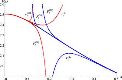
Figure 1: [Left] The function $F(g)=\int_{-\infty}^{\infty}dx\ e^{-x^{2}/2-g^{2}x^{4}}$ (black solid), its weak coupling expansions $F_{s}^{(N_{s})}(g)$ (red dotted) and strong coupling expansions $F_{l}^{(N_{l})}(g)$ (blue dashed) are plotted to $g$. [Right] The differences between the interpolating functions $F_{m,n}^{(\alpha)}(g)$ and $F(g)$ normalized by $F(g)$ are plotted to $g$ (solid), with $(F_{s}^{(20)}(g)-F)/F$ (red dotted) and $(F_{l}^{(20)}(g)-F)/F$ (blue dashed).

Let us demonstrate “the landscape problem of interpolating functions” in the example

$$F(g)=\int_{-\infty}^{\infty}dx\ e^{-\frac{x^{2}}{2}-g^{2}x^{4}}=\frac{e^{\frac{1}{32g^{2}}}}{2\sqrt{2}g}K_{\frac{1}{4}}\left(\frac{1}{32g^{2}}\right),$$ (2.12)

which is the partition function of the zero-dimensional $\varphi^{4}$ theory. Here $K_{n}(z)$ is the modified Bessel function of the second kind. The function $F(g)$ has the following weak and strong coupling expansions:

$$F_{s}^{(N_{s})}(g)=\sum_{k=0}^{N_{s}}s_{k}g^{k},\quad s_{2k+1}=0,\quad s_{2k}=\frac{\sqrt{2}\Gamma(2k+1/2)}{k!}(-4)^{k},\mbox{$$}$$

$$F_{l}^{(N_{l})}(g)=\frac{1}{\sqrt{g}}\sum_{k=0}^{N_{l}}l_{k}g^{-k},\quad l_{k}=\frac{\Gamma\left(\frac{k}{2}+\frac{1}{4}\right)}{2k!}\left(-\frac{1}{2}\right)^{k}.$$ (2.13)

In fig. 1 [Left], we plot $F(g)$, $F_{s}^{(N_{s})}(g)$ and $F_{l}^{(N_{l})}(g)$ for some $N_{s}$ and $N_{l}$. We see that as increasing $N_{s}(N_{l})$, the weak (strong) coupling expansion blows up at smaller $g$ (larger $1/g$). This can be understood from that the weak coupling expansion is asymptotic while the strong coupling expansion converges everywhere as seen in (2.13).

We can construct various interpolating functions of $F(g)$, whose explicit forms are given in appendix B.1. In terms of the FPR interpolating function $F_{m,n}^{(\alpha)}(g)$, we plot

$$\frac{F_{m,n}^{(\alpha)}(g)-F(g)}{F(g)},$$

for some values of $(m,n,\alpha)$ in fig. 1 [Right]. At first sight, this plot shows that the interpolating functions with larger $(m,n)$ roughly tend to give better approximations of $F(g)$ as naively expected. However, we observe an exception of this tendency and somewhat unclear point. The exception is that $F_{1,1}^{(1/2)}(g)$ is closer than $F_{2,2}^{(1/10)}(g)$ to $F(g)$. The unclear point is that if we consider the same value of $(m,n)$ but different values of $\alpha$, then precisions of some interpolating functions are fairly different from each other, e.g., the maximal value of $|F_{2,2}^{(1/10)}(g)-F|/F$ is 0.0188286 while the one of $|F_{2,2}^{(1/2)}(g)-F|/F$ is 0.000853566. These facts lead us to the following important question. When we do not know an explicit form of a function $F(g)$ but know its small-$g$ and large-$g$ expansions, how do we choose the best approximation of $F(g)$ among its interpolating functions?

In next section, we propose a criterion to determine the best interpolating functions, which covers a wide class of problem. In section 4, we will come back to the above example and check that our criterion correctly determines the best interpolating function as well as other more nontrivial examples.

3 Criterion for the “best” interpolating function

In the previous section, we have seen that we can construct enormous interpolating functions of a function $F(g)$ in principle. As demonstrated, then we have encountered “the landscape problem of interpolating functions”, i.e., it is unclear how one determines the best approximation of $F(g)$ among interpolating functions without knowing an explicit form of $F(g)$. In this section, we construct a criterion to choose the best interpolating function by using information on the small-$g$ and large-$g$ expansions. We also mention some limitations of our criterion.

Suppose a function $F(g)$ and that we know its power series expansions around $g=0$ up to $\mathcal{O}(g^{a+N_{s}+1})$ and around $g=\infty$ up to $\mathcal{O}(g^{b-N_{l}-1})$. Namely, we have explicit forms of $F_{s}^{(N_{s})}(g)$ and $F_{l}^{(N_{l})}(g)$. Then we consider a test function $G(g)$, which would approximate $F(g)$ such as interpolating functions. Given the test function $G(g)$, let us introduce the two quantities

$$I_{s}[G]=\int_{0}^{g_{s}^{\ast}}dg\left|G(g)-F_{s}^{(N_{s}^{\ast})}(g)\right|,\quad I_{l}[G]=\int_{g_{l}^{\ast}}^{\Lambda}dg\left|G(g)-F_{l}^{(N_{l}^{\ast})}(g)\right|,$$ (3.1)

where the parameter $\Lambda$ in $I_{l}[G]$ is the cutoff of the integration to make $I_{l}[G]$ well-defined and hence taken to be large. Throughout this paper, we take $\Lambda=1000$. The parameters $g_{s}^{\ast},g_{l}^{\ast},N_{s}^{\ast}$ and $N_{l}^{\ast}$ will be defined shortly. Roughly speaking, these are taken such that $F_{s}^{(N_{s}^{\ast})}(g)$ and $F_{l}^{(N_{l}^{\ast})}(g)$ are sufficiently close to $F(g)$ for $0\leq g\leq g_{s}^{\ast}$ and $g\geq g_{l}^{\ast}$, respectively. Then we propose that $I_{s}[G]$ and $I_{l}[G]$ measure precision of approximation of $F(g)$ by the test function $G(g)$. In other words, we expect that the “best” interpolating function $G_{\rm best}(g)$ minimizes a value of $I_{s}[G]$ plus $I_{l}[G]$ among candidates of interpolating functions:

$$I_{s}[G_{\rm best}]+I_{l}[G_{\rm best}]=\min{\left\{I_{s}[G]+I_{l}[G]\right\}}.$$ (3.2)

Now we define the parameters $g_{s}^{\ast},g_{l}^{\ast},N_{s}^{\ast}$ and $N_{l}^{\ast}$. Actually we differently take these values depending on properties of the small-$g$ and large-$g$ expansions. We classify the expansions into the following four types.

1. The both small-$g$ and large-$g$ expansions are convergent.

2. The small-$g$ expansion is asymptotic while the large-$g$ expansion is convergent.

3. The small-$g$ expansion is convergent while the large-$g$ expansion is asymptotic.

4. The both small-$g$ and large-$g$ expansions are asymptotic.

Although we cannot determine whether the expansions are convergent or not for finite $N_{s}$ and $N_{l}$ in principle, we can often extrapolate the finite data of the coefficients to infinite $N_{s}$ and $N_{l}$ as we will demonstrate in some examples. In the rest of this section, we explain how to choose the parameters $g_{s}^{\ast},g_{l}^{\ast},N_{s}^{\ast}$ and $N_{l}^{\ast}$ for the above four types.

Type 1: convergent small-$g$ and large-$g$ expansions

Suppose that the small-$g$ and large-$g$ expansions are convergent inside the circle $|g|=g_{s}^{c}$ and outside the circle $|g|=g_{l}^{c}$, respectively. First, we assume that $N_{s},$ and $N_{l}$ are sufficiently large for a simplicity of explanation. Then we will relax this condition later.

For $N_{s}\gg 1$, the small-$g$ expansion $F_{s}^{(N_{s})}(g)$ should be very close to $F(g)$ for $|g|<g_{s}^{c}$ up to non-perturbative effect in a sense of $g$ such as $\sim e^{-1/g}$. Correspondingly, for $N_{l}\gg 1$, the large-$g$ expansion $F_{l}^{(N_{l})}(g)$ is also very close to $F(g)$ for $|g|>g_{l}^{c}$ up to non-perturbative effect in a sense of $1/g$ such as $\sim e^{-g}$. Hence if we take $0<g_{s}^{\ast}<g_{s}^{c}$ and $N_{s}^{\ast}=N_{s}$ in (3.1), then sufficiently small value of $I_{s}[G]$ implies that $G(g)$ is almost $F(g)$ in the region $0\leq g\leq g_{s}^{\ast}$ up to the non-perturbative effect of the $g$-expansion. Similarly, taking $g_{l}^{\ast}>g_{l}^{c}$ and $N_{l}^{\ast}=N_{l}$, the condition $I_{l}[G]\ll 1$ means that $G(g)$ approximates $F(g)$ very well for $g\geq g_{l}^{\ast}$ up to the non-perturbative effect of the $1/g$-expansion. Thus if we also impose values of $g_{s}^{\ast}$ and $g_{l}^{\ast}$ such that the non-perturbative effects are negligible for $0\leq g\leq g_{s}^{\ast}$ and $g\geq g_{l}^{\ast}$, then the test function $G(g)$ satisfying $I_{s}[G]\ll 1$ and $I_{l}[G]\ll 1$ is sufficiently close to the function $F(g)$ in these domains. Note that although imposing only $I_{s}[G]\ll 1$ has the non-perturbative ambiguity in the sense of the small-$g$ expansion, this ambiguity would be partially fixed by imposing $I_{l}[G]\ll 1$, and vice versa as demonstrated in the last of this subsection.

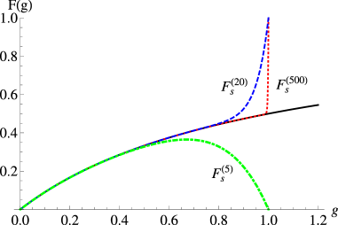
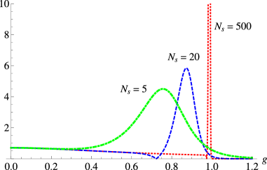
Figure 2: [Left] The function $F(g)=g/(1+g)$ and its small $g$ expansions $F_{s}^{(N_{s})}$ are plotted to $g$. [Right] The magnitudes of the curvatures of $F_{s}^{(N_{s})}$ are plotted against $g$.

Now let us relax the conditions $N_{s},N_{l}\gg 1$. When $N_{s}$ is sufficiently large but finite, the small-$g$ expansion $F_{s}^{(N_{s})}(g)$ blows up at almost $g=g_{s}^{c}$. As decreasing $N_{s}$, this blow up point, say $g_{s}^{b}$, becomes smaller (see fig. 2 [Left]). In the region $g>g_{s}^{b}$, the small-$g$ expansion is obviously no longer close to the function $F(g)$ even if we are inside of the convergent radius. Similarly this is true also for the large-$g$ expansion. The locations of the blow-up points $g_{s}^{b}$ and $g_{l}^{b}$ can be found by studying their curvatures of $F_{s}^{(N_{s})}(g)$ and $F_{l}^{(N_{l})}(g)$, respectively, because these points have very large curvatures around $g=g_{s}^{b}$ and $g=g_{l}^{b}$ as demonstrated in fig. 2 [Right].

As a conclusion, we choose the parameters $N_{s}^{\ast}$ and $N_{l}^{\ast}$ as

$$N_{s}^{\ast}=N_{s},\quad N_{l}^{\ast}=N_{l}.$$ (3.3)

We take $g_{s}^{\ast}$ and $g_{l}^{\ast}$ such that

• $g_{s}^{\ast}$ and $g_{l}^{\ast}$ satisfy

  $$0<g_{s}^{\ast}<g_{s}^{b},\quad g_{s}^{\ast}<g_{s}^{c},\quad g_{l}^{\ast}>g_{l}^{b},\quad g_{l}^{\ast}>g_{l}^{c}.$$ (3.4)

• The non-perturbative effects are ignorable for $0\leq g\leq g_{s}^{\ast}$ and $g\geq g_{l}^{\ast}$.

• The regions $0\leq g\leq g_{s}^{\ast}$ and $g\geq g_{l}^{\ast}$ are as wide as possible with satisfying the above two conditions.

Type 2: asymptotic small-$g$ expansion and convergent large-$g$ expansion

Suppose that the small-$g$ expansion is asymptotic but the large-$g$ expansion is convergent. Then, while we take the parameters $g_{l}^{\ast}$ and $N_{l}^{\ast}$ as in type 1, we differently take $g_{s}^{\ast}$ and $N_{s}^{\ast}$ for this case.

Before going to explain this, we shall recall “optimization” of asymptotic series. Let us consider a function $F(g)$ and its power series expansion $F_{s}^{(N_{s})}(g)$ around $g=0$. If this expansion is asymptotic and non-convergent, $F_{s}^{(\infty)}(g)$ diverges. We would like to know which value of $N_{s}$ optimally approximates $F(g)$ with fixed $g$. Such optimization is usually achieved by minimization of the last term of the asymptotic series (see e.g. [8]). Namely, the optimized value $N_{s}^{o}$ is determined by the condition

$$\left.\frac{\partial}{\partial k}\log{s_{k}}\right|_{k=N_{s}^{o}}+\log{g}=0.$$ (3.5)

We can also estimate “error” of this optimization by the next term of the series:

$$\delta_{s}(g)=\left|s_{N_{s}^{o}+1}g^{a+N_{s}^{o}+1}\right|.$$ (3.6)

Thus we choose $N_{s}^{\ast}$ and $N_{l}^{\ast}$ in (3.1) as

$$N_{s}^{\ast}=N_{s}^{o},\quad N_{l}^{\ast}=N_{l}.$$ (3.7)

We take $g_{s}^{\ast}$ and $g_{l}^{\ast}$ such that

• $g_{s}^{\ast}$ and $g_{l}^{\ast}$ satisfy

  $$\delta_{s}(g_{s}^{\ast})\leq\epsilon_{s}\ll 1,\quad g_{l}^{\ast}>g_{l}^{b},\quad g_{l}^{\ast}>g_{l}^{c}.$$ (3.8)

• The non-perturbative effects are ignorable for $0\leq g\leq g_{s}^{\ast}$ and $g\geq g_{l}^{\ast}$.

• The regions $0\leq g\leq g_{s}^{\ast}$ and $g\geq g_{l}^{\ast}$ are as wide as possible.

Since $\delta_{s}(g)$ is monotonically increasing, the above condition $\delta_{s}(g_{s}^{\ast})\leq\epsilon_{s}$ means $\delta_{s}(g)\leq\epsilon_{s}\ll 1$ for $0\leq g\leq g_{s}^{\ast}$. Here the value of $\epsilon_{s}$ are taken depending on desired precision.

Type 3: convergent small-$g$ expansion and asymptotic large-$g$ expansion

This case is quite parallel to type 2. The optimized order $N_{l}^{o}$ of the large-$g$ expansion is determined by

$$\left.\frac{\partial}{\partial k}\log{l_{k}}\right|_{k=N_{l}^{o}}-\log{g}=0,$$ (3.9)

with the error

$$\delta_{l}(g)=\left|l_{N_{l}^{o}+1}g^{b-N_{l}^{o}-1}\right|.$$ (3.10)

Thus we take $N_{s}^{\ast}$ and $N_{l}^{\ast}$ as

$$N_{s}^{\ast}=N_{s},\quad N_{l}^{\ast}=N_{l}^{o}.$$ (3.11)

The parameters $g_{s}^{\ast}$ and $g_{l}^{\ast}$ are taken such that

• $g_{s}^{\ast}$ and $g_{l}^{\ast}$ satisfy

  $$0<g_{s}^{\ast}<g_{s}^{b},\quad g_{s}^{\ast}<g_{s}^{c},\quad\delta_{l}(g_{l}^{\ast})\leq\epsilon_{l}\ll 1.$$ (3.12)

• The non-perturbative effects are ignorable for $0\leq g\leq g_{s}^{\ast}$ and $g\geq g_{l}^{\ast}$.

• The regions $0\leq g\leq g_{s}^{\ast}$ and $g\geq g_{l}^{\ast}$ are as wide as possible.

Since $\delta_{l}(g)$ is the monotonically decreasing function of $g$, the condition $\delta_{l}(g_{l}^{\ast})\leq\epsilon_{l}$ means $\delta_{l}(g)\leq\epsilon_{l}\ll 1$ in the region $g\geq g_{l}^{\ast}$. Here we take the value of $\epsilon_{l}$ depending on desired precision as $\epsilon_{s}$.

Type 4: asymptotic small-$g$ and large-$g$ expansions

When the both series are asymptotic, we take

$$N_{s}^{\ast}=N_{s}^{o},\quad N_{l}^{\ast}=N_{l}^{o}.$$ (3.13)

The parameters $g_{s}^{\ast}$ and $g_{l}^{\ast}$ are taken to be

• $g_{s}^{\ast}$ and $g_{l}^{\ast}$ satisfy

  $$\delta_{s}(g_{s}^{\ast})\leq\epsilon_{s},\quad\delta_{l}(g_{l}^{\ast})\leq\epsilon_{l}.$$ (3.14)

• The non-perturbative effects are ignorable for $0\leq g\leq g_{s}^{\ast}$ and $g\geq g_{l}^{\ast}$.

• The regions $0\leq g\leq g_{s}^{\ast}$ and $g\geq g_{l}^{\ast}$ are as wide as possible.

Remarks

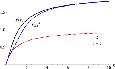
Figure 3: The function $F(g)=g/(1+g)+e^{-1/g}$ and its perturbative part $g/(1+g)$ in the sense of $g$ are plotted to $g$. Hence the deviation between them shows purely the non-perturbative effect $e^{-1/g}$. We see that the Padé approximant $F_{2,2}^{(-1)}(g)=g(4g^{2}/5-4g/5+1)/(2g^{3}/5+g/5+1)$ of $F(g)$ partially knows about the non-perturbative effect.

As a simple example, let us consider the function

$$F(g)=\frac{g}{1+g}+ce^{-\frac{1}{g}},$$ (3.15)

with a constant $c$. Clearly the function $F(g)$ has the convergent small-$g$ and large-$g$ expansions. Since the second term is non-perturbative in a sense of $g$, the small-$g$ expansion is independent of $c$. Therefore only imposing $I_{s}[G]\ll 1$ with $g_{s}^{\ast}<g_{s}^{c}(=1)$ and $e^{-1/g_{s}^{\ast}}\ll 1$ is insufficient to check whether $G(g)$ nicely approximates $F(g)$ including the non-perturbative effect or not. Namely, we should also require $I_{l}[G]\ll 1$ to fix the non-perutbative ambiguity of the approximation as depicted in fig. 3.

Next, suppose the example

$$F(g)=\frac{g}{1+g}+c_{1}e^{-\frac{1}{g}}+c_{2}e^{-g}+c_{3}e^{-g-\frac{1}{g}},$$ (3.16)

whose expansions around $g=0$ and $g=\infty$ are also convergent. While the small-$g$ expansion has information on the 1st and 3rd terms, the large-$g$ expansion has information on the 1st and 2nd terms. Note that the both expansions never know about the last term. This exhibits limitations of our interpolating functions and criterion, i.e., our criterion never fix the ambiguity of mixed non-perturbative effects such as $e^{-g-1/g}$, which are non-perturbative in senses of both $g$ and $1/g$. Although the above examples correspond to type 1, we expect that this feature is true also for the other types.

4 Some examples

In this section, we explicitly check that our criterion proposed in section 3 works for the partition function of the zero-dimensional $\varphi^{4}$ theory, specific heat in the 2d Ising model, average plaquette in the 4d $SU(3)$ pure Yang-Mills theory on lattice and free energy in the $c=1$ string theory at self-dual radius.

4.1 Partition function of zero-dimensional $\varphi^{4}$ theory

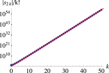
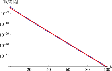
Figure 4: [Left] The weak coupling expansion coefficients $|s_{2k}|$ divided by $k!$ is plotted to $k$ in semi-log scale. The straight line shows fitting by the linear function $\log{(|s_{2k}|/k!)}=\log{c_{s}}+k\log{A_{s}}$. [Right] The strong coupling expansion coefficients $|l_{k}|$ multiplied by $\Gamma(k/2)$ is plotted against $k$ in semi-log scale. The straight line denotes the linear fitting $\log{(\Gamma(k/2)|l_{k}|)}=\log{c_{l}}+k\log{A_{l}}$.

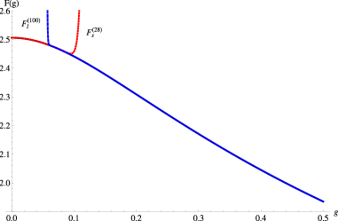
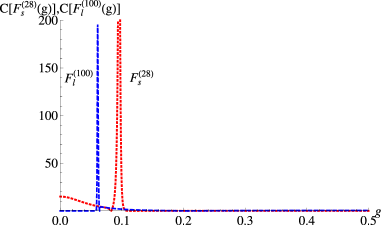
Figure 5: [Left] $F(g)$ (black solid), $F_{s}^{(28)}(g)$ (red dotted) and $F_{l}^{(100)}(g)$ (blue dashed) are plotted to $g$. [Right] The absolute values of the curvatures of $F_{s}^{(28)}(g)$ (red dotted) and $F_{l}^{(100)}(g)$ (blue dashed) are plotted to $g$.

Let us come back to the example (2.12) appearing in section 2.4:

$$F(g)=\int_{-\infty}^{\infty}dx\ e^{-\frac{x^{2}}{2}-g^{2}x^{4}}.$$

We can easily see from (2.13) that the weak coupling expansion is asymptotic while the strong one is convergent. Hence this problem corresponds to type 2.

Although we know all the coefficients of the both expansions for this case, in more practical situations, we usually have their small-$g$ and large-$g$ expansions up to only finite orders. As an exercise of such practical situations, let us restrict that we know only the first 101 coefficients for a practical purpose, i.e., we have only information on $F_{s}^{(100)}$ and $F_{l}^{(100)}$. Then we will estimate large order behaviors of the coefficients by extrapolation in terms of the finite data.

Determination of $g_{s}^{\ast}$

First let us study large order behavior of the weak coupling expansion. In fig. 4 [Left], we plot how the coefficients $s_{2k}$ behave as increasing $k$. From this plot, we find that the coefficient in large $k$ regime grows as

$$\frac{|s_{2k}|}{k!}\sim c_{s}A_{s}^{k},\quad{\rm with}\ c_{s}=0.0620840\ {\rm and}\ A_{s}=15.4189.$$ (4.1)

Since the coefficient grows by the factorial, the weak coupling expansion is asymptotic. By performing optimization (3.5), we find

$$N_{s}^{o}=\frac{2}{A_{s}g^{2}},\quad\delta_{s}(g)=c_{s}e^{-\frac{1}{A_{s}g^{2}}}.$$ (4.2)

Taking $\epsilon_{s}=10^{-7}$ in (3.8), we find

$$N_{s}^{\ast}=N_{s}^{o}=28,\quad g_{s}^{\ast}=0.0680628.$$ (4.3)

Determination of $g_{l}^{\ast}$

	$\Lambda^{-1}\int dg\bigl{|}\frac{(F_{m,n}^{(\alpha)}-F}{F}\bigr{|}$	$I_{s}[F_{m,n}^{(\alpha)}]$	$I_{l}[F_{m,n}^{(\alpha)}]$	$I_{s}+I_{l}$
$F_{0,0}^{(1/2)}$	0.000659728	0.00446072	0.381344	0.385805
$F_{1,1}^{(1/2)}$	$9.27801\times 10^{-6}$	0.000297906	0.0142222	0.0145201
$F_{1,1}^{(1/6)}$	0.0000760393	0.000432581	0.106287	0.106720
$F_{2,2}^{(1/2)}$	$4.61177\times 10^{-7}$	0.0000230059	0.000849124	0.000872130
$F_{2,2}^{(1/6)}$	$5.24010\times 10^{-6}$	0.0000450000	0.00905419	0.00909919
$F_{2,2}^{(1/10)}$	0.0000235129	0.0000430012	0.0373156	0.0373586
$F_{3,3}^{(1/2)}$	$2.96944\times 10^{-8}$	$1.94617\times 10^{-6}$	0.0000576043	0.0000595505
$F_{3,3}^{(1/6)}$	$3.84001\times 10^{-7}$	$5.09656\times 10^{-6}$	0.000738006	0.000743103
$F_{3,3}^{(1/14)}$	$8.84054\times 10^{-6}$	$2.59016\times 10^{-6}$	0.0148826	0.0148852
$\bf F_{4,4}^{(1/2)}$	$\bf 2.17241\times 10^{-9}$	$\bf 1.78480\times 10^{-7}$	$\bf 4.25411\times 10^{-6}$	$\bf 4.43259\times 10^{-6}$
$F_{4,4}^{(1/6)}$	$2.85852\times 10^{-8}$	$5.50786\times 10^{-7}$	0.0000577750	0.0000583258
$F_{4,4}^{(1/10)}$	$5.77057\times 10^{-7}$	$1.52640\times 10^{-6}$	0.00111431	0.00111584
$F_{4,4}^{(1/18)}$	$3.17581\times 10^{-6}$	$8.72352\times 10^{-7}$	0.00549043	0.00549131

Table 1: Result on the zero-dimensional $\varphi^{4}$ theory.

Next we estimate large order behavior of the strong coupling expansion. In fig. 4 [Right], we plot $\Gamma(k/2)|l_{k}|$ against $k$ in semi-log scale. Then fitting the data leads us to

$$\Gamma(k/2)|l_{k}|\sim c_{l}A_{l}^{k},\quad{\rm with}\ c_{l}=0.0769534\ {\rm and}\ A_{l}=0.243235.$$ (4.4)

This shows that the strong coupling expansion is convergent with the infinite convergent radius. Since the strong coupling expansion $F_{l}^{(100)}$ behaves as $\sim g^{-201/2}$ in small $g$ regime, this blows up at some point as seen in fig. 5 [Left]. In order to look for the blow-up point, we study the magnitude of the curvature:

$$C[f(g)]=\Bigl{|}\frac{f^{\prime\prime}(g)}{\left(1+(f^{\prime}(g))^{2}\right)^{3/2}}\Bigr{|}.$$ (4.5)

In fig. 5 [Right], we plot the curvature of $F_{l}^{(100)}(g)$ to $g$. From this plot, we find the sharp peak of $C[F_{l}^{(100)}]$ around $g=0.0607430$ and thus we take

$$g_{l}^{\ast}=0.1.$$ (4.6)

Result

Now we are ready to test our criterion for the “best” interpolating function. We measure precision of the interpolating function $F_{m,n}^{(\alpha)}(g)$ by

$$\frac{1}{\Lambda}\int_{0}^{\Lambda}dg\Bigl{|}\frac{F_{m,n}^{(\alpha)}(g)-F(g)}{F(g)}\Bigr{|},$$ (4.7)

which should be minimized by the best interpolating function. Comparing this with values of $I_{s}[F_{m,n}^{(\alpha)}]$ and $I_{l}[F_{m,n}^{(\alpha)}]$, we can test our criterion (3.2) proposed in the previous section. We summarize our result in tab. 1. We easily see that the interpolating function $F_{4,4}^{(1/2)}(g)$ gives the most precise approximation of $F(g)$ among the interpolating functions in the table. Note that $F_{4,4}^{(1/2)}(g)$ has also the minimal values of $I_{s}$ and $I_{l}$ among the candidates. This shows that our criterion correctly chooses the best interpolating function in this example.

4.2 Specific heat in two-dimensional Ising model

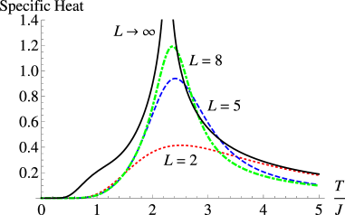
Figure 6: The specific heat in the 2d Ising model is plotted to $T/J$ for various lattice sizes.

Let us consider the 2d Ising model on the $L\times L$ square lattice with periodic boundary condition. We can study interpolation problem between high and low temperature expansions in this model. It is well known that this system in the $L\rightarrow\infty$ limit exhibits the second order phase transition and the specific heat has a singularity as depicted in fig. 6. On the contrary, our interpolating function (2.7) gives a smooth function unless this has poles. Hence we expect that our interpolating function fails to approximate the specific heat in the infinite volume limit while it should work for finite $L$. Thus it is interesting to study how properties of interpolating function change as increasing $L$.

The Hamiltonian of the 2d Ising model is given by

$$H=-J\sum_{(\mathbf{x},\mathbf{y})\in{\rm neighbor}}\sigma_{\mathbf{x}}\sigma_{\mathbf{y}},$$ (4.8)

where $\sigma_{\mathbf{x}}$ is the spin variable at the position $\mathbf{x}$ taking the values $\pm 1$ and $J$ is the coupling constant. In terms of the temperature $T$, we define the partition function of this model by

$$Z_{L}(K)=\sum_{\{\rm state\}}e^{-\frac{1}{T}H}=\sum_{\{\rm state\}}e^{K\sum_{(\mathbf{x},\mathbf{y})}\sigma_{\mathbf{x}}\sigma_{\mathbf{y}}},\quad{\rm with}\ K=\frac{J}{T}.$$ (4.9)

The exact solution of the partition function is given by (see e.g. [9])

$$Z_{L}(K)=\frac{1}{2}\left(S_{11}(K)+2S_{10}(K)-S_{00}(K)\right),\mbox{$$}$$

$$S_{\sigma_{1}\sigma_{2}}(K)=2^{L^{2}}\prod_{p,q=0}^{L-1}\Bigl{[}\cosh^{2}{(2K)}-\sinh{(2K)}\Bigl{(}\cos{\frac{(2p+\sigma_{1})\pi}{L}}+\cos{\frac{(2q+\sigma_{2})\pi}{L}}\Bigr{)}\Bigr{]}^{\frac{1}{2}}.$$ (4.10)

Let us introduce the quantity

$$C_{L}(K)=\frac{1}{L^{2}}\frac{\partial^{2}}{\partial K^{2}}\log{Z_{L}(K)},$$ (4.11)

which gives the specific heat by $K^{2}C_{L}(K)$. Since the partition function is a power series of $e^{K}$, we see that high temperature expansion around $K=0$ of $C_{L}(K)$ is a power series of $K$ while low temperature expansion around $K=\infty$ gives a power series of $e^{-K}$. In order to make the both expansions the power series form (2.1), we introduce the parameter $g$ by

$$e^{2K}=1+g.$$ (4.12)

Then the high and low temperature expansions of $C_{L}(g)$ become power series of $g$ and $1/g$, respectively. Namely, the small-$g$ and large-$g$ expansions in the previous sections correspond to the high and low temperature expansions, respectively. Note that $C_{L}(g)$ is a rational function of $g$ for arbitrary finite $L$. Therefore one of the Padé approximants should give the exact answer for finite $L$ in principle.

Below we consider interpolation problem for $L=2,5,8$ and $\infty$. Denoting the high and low temperature expansions as

$$C_{s}^{(N_{s})}=g^{a}\sum_{k=0}^{N_{s}}s_{k}g^{k},\quad C_{l}^{(N_{l})}=g^{b}\sum_{k=0}^{N_{l}}l_{k}g^{-k},$$ (4.13)

we also assume that we have information only on the high temperature expansion $C_{s}^{(50)}(g)$ and low temperature expansion $C_{l}^{(50)}(g)$. For all the cases below, we explicitly write down explicit formulas for interpolating functions $C_{m,n}^{(\alpha)}(g)$ taking the FPR form (2.7) in app. B.2.

4.2.1 $2\times 2$ lattice

For $L=2$, the function $C_{2}(g)$ has the following expansions

$$C_{2}(g) = 4+8g^{2}-8g^{3}-30g^{4}+\mathcal{O}(g^{5})\mbox{$$}$$ (4.14)

$$= g^{-4}\left(96-384g^{-1}+960g^{-2}-1920g^{-3}+2272g^{-4}+\mathcal{O}(g^{-5})\right).$$

In terms of these expansions, we can construct various interpolating functions for $C_{2}(g)$. As in the previous example, we read large order behaviors of the both expansions by extrapolation. By fitting the data of $s_{k}$ and $l_{k}$ for $k=10\sim 50$, we find

$$|s_{k}|\sim c_{s}A_{s}^{k},\quad{\rm with}\ c_{s}=8.38769\ {\rm and}\ A_{s}=1.4614,\mbox{$$}$$

$$|l_{k}|\sim c_{l}A_{l}^{k},\quad{\rm with}\ c_{l}=154.976\ {\rm and}\ A_{l}=2.4487.$$ (4.15)

Hence the high and low temperature expansions seem to be convergent for $|g|<A_{s}^{-1}=0.684275$ and $|g|>A_{l}$, respectively. We also find the blow-up points of $F_{s}^{(50)}(g)$ and $F_{l}^{(50)}(g)$ at $g=g_{s}^{b}=0.453215$ and $g=g_{l}^{b}=2.59736$, respectively. Thus we take

$$N_{s}^{\ast}=50,\quad g_{s}^{\ast}=0.3,\quad N_{l}^{\ast}=50,\quad g_{l}^{\ast}=2.8.$$ (4.16)

We summarize our result in fig. 7 and tab. 2. We find that our criterion correctly determines the best interpolating function $C_{7,6}^{(-1)}(g)$ among the candidates as in the previous example.

	$\Lambda^{-1}\int dg\bigl{|}\frac{C_{m,n}^{(\alpha)}-C_{2}}{C_{2}}\bigr{|}$	$I_{s}[C_{m,n}^{(\alpha)}]$	$I_{l}[C_{m,n}^{(\alpha)}]$	$I_{s}+I_{l}$
$C_{1,1}^{(-4)}$	0.00224809	0.0912750	0.102638	0.193913
$C_{1,1}^{(-4/3)}$	0.000817041	0.0617656	0.0193989	0.0811645
$C_{1,2}^{(-2)}$	0.00100228	0.0751219	0.0466568	0.121779
$C_{1,2}^{(-1)}$	0.000286070	0.058021	0.00257514	0.0605961
$C_{2,2}^{(-4)}$	0.000173889	0.00768450	0.00852503	0.0162095
$C_{2,3}^{(-2)}$	0.000158806	0.00224879	0.00550386	0.00775265
$C_{3,2}^{(-2)}$	0.000322997	0.00658097	0.0116865	0.0182674
$C_{3,4}^{(-1)}$	0.0000147709	0.000148814	0.000258785	0.000407598
$C_{4,3}^{(-2)}$	0.000168121	0.00345741	0.00565649	0.0091139
$C_{4,3}^{(-1)}$	0.0000651441	0.00156065	0.00170668	0.00326733
$C_{5,4}^{(-1)}$	0.0000207392	0.000525855	0.000327812	0.000853666
$C_{6,5}^{(-1)}$	0.0000119340	0.000174690	0.000192164	0.000366854
$\bf C_{7,6}^{(-1)}$	$\bf 1.22853\times 10^{-6}$	$\bf 3.39663\times 10^{-6}$	$\bf 0.0000523107$	0.0000557073
$C_{6,7}^{(-1)}$	0.0000128648	0.000129274	0.0000598797	0.000189154

Table 2: Result for $L=2$

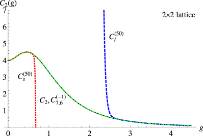
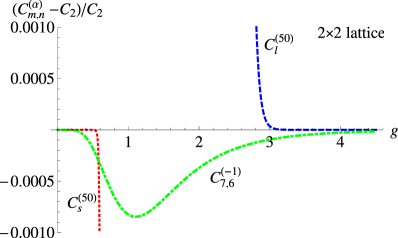
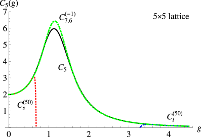
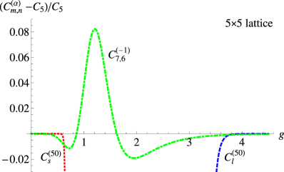
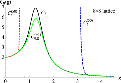
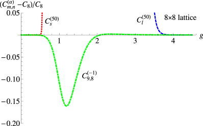
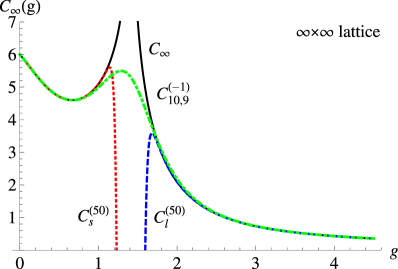
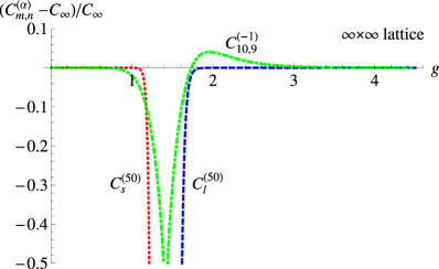
Figure 7: [Left] The function $C_{L}(g)$ (black solid), the best interpolating function (green dot-dashed), its high (red dotted) and low (blue dashed) temperature expansions are plotted to $g$ for each $L$. [Right] $|(C_{m,n}^{(\alpha)}-C_{L})/C_{L}|$ (green dot-dashed), $|(C_{s}^{(50)}-C_{L})/C_{L}|$ (red dotted) and $|(C_{l}^{(50)}-C_{L})/C_{L}|$ (blue dashed) are plotted against $g$ for each $L$.

4.2.2 $5\times 5$ lattice

	$\Lambda^{-1}\int dg\bigl{|}\frac{C_{m,n}^{(\alpha)}-C_{5}}{C_{5}}\bigr{|}$	$I_{s}[C_{m,n}^{(\alpha)}]$	$I_{l}[C_{m,n}^{(\alpha)}]$	$I_{s}+I_{l}$
$C_{1,1}^{(-4)}$	0.00447397	0.0908906	0.0573872	0.148278
$C_{1,1}^{(-4/3)}$	0.00228464	0.0639680	0.0237879	0.0877559
$C_{1,2}^{(-2)}$	0.00265831	0.0726585	0.0320523	0.104711
$C_{1,2}^{(-1)}$	0.00164725	0.0540871	0.0113251	0.0654122
$C_{2,2}^{(-4)}$	0.00142494	0.0137917	0.0102147	0.0240064
$C_{2,3}^{(-2)}$	0.00112491	0.00956534	0.00538250	0.0149478
$C_{2,3}^{(-1)}$	0.00137710	0.0372464	0.00707500	0.0443214
$C_{3,2}^{(-2)}$	0.000961824	0.00689287	0.00279760	0.00969046
$C_{3,3}^{(-4)}$	0.00113015	0.00776624	0.00559209	0.0133583
$C_{3,3}^{(-4/7)}$	0.00143699	0.000319958	0.0237685	0.0240885
$C_{3,4}^{(-2)}$	0.00100163	0.00699082	0.00374339	0.0107342
$C_{3,4}^{(-1)}$	0.000721790	0.00555444	0.00130205	0.00685649
$C_{4,3}^{(-1)}$	0.000469692	0.00359619	0.00281633	0.00641253
$C_{4,4}^{(-4/9)}$	0.00294461	0.00712618	0.0459126	0.0530387
$C_{4,5}^{(-1)}$	0.000596309	0.00398025	0.000648710	0.00462896
$C_{6,5}^{(-1)}$	0.000440902	0.00134450	0.000398831	0.00174333
$\bf C_{7,6}^{(-1)}$	$\bf 0.0000555327$	$\bf 0.000123232$	$\bf 0.0000416657$	0.000164898
$C_{6,7}^{(-1)}$	0.0000898635	0.000325997	0.0000649638	0.000390961

Table 3: Result for $L=5$

Next we consider $5\times 5$ lattice. For this case, $C_{5}(g)$ has the following expansions

$$C_{5}(g) = 2+\frac{5g^{2}}{2}-\frac{3g^{3}}{2}+\frac{17g^{4}}{8}+\mathcal{O}\left(g^{5}\right),\mbox{$$}$$ (4.17)

$$= g^{-4}\left(64-256g^{-1}+928g^{-2}-3008g^{-3}+9440g^{-4}+\mathcal{O}(g^{-5})\right).$$

By fitting the data of $s_{k}$ and $l_{k}$ for $k=10\sim 50$, we again find

$$|s_{k}|\sim c_{s}A_{s}^{k},\quad {\rm with}\ c_{s}=0.980413\ {\rm and}\ A_{s}=1.60585,\mbox{$$}$$

$$|l_{k}|\sim c_{l}A_{l}^{k},\quad {\rm with}\ c_{l}=98.4806\ {\rm and}\ A_{l}=3.21044.$$ (4.18)

Hence the high and low temperature expansions seem to be convergent for $|g|<A_{s}^{-1}=0.622724$ and $|g|>A_{l}$, respectively. We also find the blow-up points $g_{s}^{b}=0.629103$ and $g_{l}^{b}=3.37946$. Thus we take the parameters in (3.1) as

$$N_{s}^{\ast}=50,\quad g_{s}^{\ast}=0.4,\quad N_{l}^{\ast}=50,\quad g_{l}^{\ast}=3.8.$$ (4.19)

Our result is summarized in fig. 7 and tab. 3. As in the $L=2$ case, we find that our criterion correctly chooses the relatively best interpolating function $C_{7,6}^{(-1)}(g)$.

There is an important difference from the $L=2$ case. Although our criterion works also for the $L=5$ case, the approximation by the best interpolation function becomes worse compared with the $L=2$ case. Indeed we have about $8\%$ discrepancy around the peak of $C_{5}(g)$. This implies that we should include information on higher order terms of the both expansions to obtain sufficiently good interpolating function. However, note that the location of the peak of the interpolating function $C_{7,6}^{(-1)}(g)$ is almost the one of $C_{5}(g)$. We actually find that $C_{7,6}^{(-1)}(g)$ and $C_{5}(g)$ have the peaks at $g=1.14765$ and $1.12930$, respectively. This point would be physically important as follows. It is known that the peak location approaches to the second order phase transition point as increasing $L$. Hence, if interpolating function for finite $L$ precisely gives the peak location of $C_{L}(g)$, then the interpolating function would be useful for finding the phase transition point. We will see in the last of this subsection that extrapolating the peak locations of the best interpolating functions for finite $L$ to infinite $L$ precisely gives the known phase transition point.

4.2.3 $8\times 8$ lattice

	$\Lambda^{-1}\int dg\bigl{|}\frac{C_{m,n}^{(\alpha)}-C_{8}}{C_{8}}\bigr{|}$	$I_{s}[C_{m,n}^{(\alpha)}]$	$I_{l}[C_{m,n}^{(\alpha)}]$	$I_{s}+I_{l}$
$C_{1,1}^{(-4)}$	0.00444636	0.0831909	0.0636770	0.146868
$C_{1,1}^{(-4/3)}$	0.00225426	0.0562683	0.0269999	0.0832682
$C_{1,2}^{(-2)}$	0.00262870	0.0649589	0.0361830	0.101142
$C_{1,2}^{(-1)}$	0.00161692	0.0463875	0.0130628	0.0594503
$C_{2,2}^{(-4)}$	0.00138694	0.00609203	0.0117589	0.0178510
$C_{2,3}^{(-2)}$	0.00108717	0.00193670	0.00627777	0.00821447
$C_{2,3}^{(-1)}$	0.00134557	0.0295467	0.00824463	0.0377913
$C_{3,2}^{(-1)}$	0.00184791	0.00144487	0.0337078	0.0351526
$C_{3,3}^{(-4)}$	0.00128215	0.00500135	0.00958245	0.0145838
$C_{3,3}^{(-4/7)}$	0.00256497	0.000826246	0.0447810	0.0456072
$C_{3,4}^{(-1)}$	0.000784632	0.00198832	0.00201671	0.00400503
$C_{4,3}^{(-1)}$	0.000587861	0.000536292	0.00191111	0.00244740
$C_{4,4}^{(-4/9)}$	0.00249203	0.00386555	0.0380123	0.0418779
$C_{4,5}^{(-1)}$	0.000673718	0.000729868	0.00107283	0.00180270
$C_{5,6}^{(-1)}$	0.000559509	0.000312770	0.000391225	0.000703995
$C_{7,6}^{(-1)}$	0.000367060	0.0000657636	0.0000453988	0.000111162
$C_{6,7}^{(-1)}$	0.000433024	0.0000980238	0.000125464	0.000223488
$C_{7,8}^{(-1)}$	0.000388259	0.0000680322	0.0000822403	0.000150272
$C_{8,7}^{(-1)}$	0.000438208	0.000175849	0.000128240	0.000304089
$C_{8,9}^{(-1)}$	0.000300809	0.0000323440	0.0000499792	0.0000823232
$\bf C_{9,8}^{(-1)}$	$\bf 0.0000987414$	$\bf 8.01947\times 10^{-6}$	$\bf 0.0000319896$	0.0000400091
$C_{9,10}^{(-1)}$	0.000209750	0.0000112848	0.0000418221	0.0000531069

Table 4: Result for $L=8$

For $8\times 8$ lattice, the high and low temperature expansions of $C_{8}(g)$ are given by

$$C_{8}(g) = 2+\frac{5g^{2}}{2}-\frac{5g^{3}}{2}+\frac{29g^{4}}{8}+\mathcal{O}(g^{5}),\mbox{$$}$$ (4.20)

$$= g^{-4}\left(64-256g^{-1}+928g^{-2}-3008g^{-3}+9440g^{-4}+\mathcal{O}(g^{-5})\right).$$

Fitting the data of $s_{k}$ and $l_{k}$ from $k=10$ to $k=50$ leads us to

$$|s_{k}|\sim c_{s}A_{s}^{k},\quad {\rm with}\ c_{s}=0.620989\ {\rm and}\ A_{s}=1.76359,\mbox{$$}$$

$$|l_{k}|\sim c_{l}A_{l}^{k},\quad {\rm with}\ c_{l}=20.5985\ {\rm and}\ A_{l}=3.44257.$$ (4.21)

Hence the high and low temperature expansions seem to converge for $|g|<A_{s}^{-1}=0.567027$ and $|g|>A_{l}$, respectively. The blow-up points are given by $g_{s}^{b}=0.522265$ and $g_{l}^{b}=3.41772$. Thus we take the parameters in (3.1) as

$$N_{s}^{\ast}=50,\quad g_{s}^{\ast}=0.4,\quad N_{l}^{\ast}=50,\quad g_{l}^{\ast}=3.7.$$ (4.22)

According to fig. 7 and tab. 4, we see again that our criterion correctly determines the best interpolating function $C_{9,8}^{(-1)}(g)$ among the candidates.

We also find the peak locations of $C_{9,8}^{(-1)}(g)$ and $C_{8}(g)$ at $g=1.27341$ and $g=1.25509$, respectively. Although the values at the peaks are different by about $16\%$, these locations are very close to each other.

4.2.4 Infinite lattice

	$\Lambda^{-1}\int dg\bigl{|}\frac{C_{m,n}^{(\alpha)}-C_{\infty}}{C_{\infty}}\bigr{|}$	$I_{s}[C_{m,n}^{(\alpha)}]$	$I_{l}[C_{m,n}^{(\alpha)}]$	$I_{s}+I_{l}$
$C_{1,1}^{(-2/3)}$	0.00275349	0.800907	0.481499	1.28241
$C_{2,1}^{(-1)}$	0.00313148	0.707807	0.514001	1.22181
$C_{2,2}^{(-2/5)}$	0.00157317	0.986636	0.462886	1.44952
$C_{2,3}^{(-1)}$	0.00165066	0.960887	0.652703	1.61359
$C_{3,4}^{(-1)}$	0.00105518	0.610940	0.357507	0.968448
$C_{4,4}^{(-2/9)}$	0.00141961	0.927616	0.538109	1.46572
$C_{4,5}^{(-1)}$	0.000963535	0.548868	0.308996	0.857864
$C_{5,5}^{(-2/11)}$	0.00145344	0.901255	0.563952	1.46521
$C_{5,6}^{(-1)}$	0.000715206	0.306906	0.194745	0.501651
$C_{6,6}^{(-2/13)}$	0.00149621	0.921327	0.582883	1.50421
$C_{6,7}^{(-1)}$	0.000400117	0.0916321	0.0596090	0.151241
$C_{7,6}^{(-1)}$	0.000304098	0.0566016	0.0188506	0.0754521
$C_{7,7}^{(-2/15)}$	0.00149432	0.899986	0.584099	1.48409
$C_{7,8}^{(-1)}$	0.000405540	0.0955453	0.0614392	0.156985
$C_{9,8}^{(-1)}$	0.000361400	0.0533636	0.0521376	0.105501
$C_{9,10}^{(-1)}$	0.000239733	0.0222130	0.0123199	0.0345328
$\bf C_{10,9}^{(-1)}$	$\bf 0.000170155$	$\bf 0.00916161$	$\bf 0.0250438$	$\bf 0.0342054$

Table 5: Result for $L\rightarrow\infty$

In the $L\rightarrow\infty$ limit, $C_{\infty}(g)=\lim_{L\rightarrow\infty}C_{L}(g)$ is given by

$$C_{\infty}(g) = \frac{16(g+1)}{\pi g(g+2)}\Biggl{[}K\left(\frac{4g(g+1)(g+2)}{\left(g^{2}+2g+2\right)^{2}}\right)-E\left(\frac{4g(g+1)(g+2)}{\left(g^{2}+2g+2\right)^{2}}\right)\mbox{$$}$$ (4.23)

$$-\left(\frac{2(g+1)}{(g+1)^{2}+1}\right)^{2}\left\{\frac{g^{4}+4g^{3}-8g-4}{\left(g^{2}+2g+2\right)^{2}}K\left(\frac{4g(g+1)(g+2)}{\left(g^{2}+2g+2\right)^{2}}\right)+\frac{\pi}{2}\right\}\Biggr{]},$$

where $K(z)$ and $E(z)$ are the complete elliptic integrals of the first and second kinds, respectively. The function $C_{\infty}(g)$ has the expansions

$$C_{\infty}(g) = 6-\frac{11g}{4}-\frac{15g^{2}}{4}+\frac{3265g^{3}}{256}-\frac{651g^{4}}{64}+\mathcal{O}(g^{5}),\mbox{$$}$$ (4.24)

$$= g^{-2}\left(16-72g^{-1}+164g^{-2}+15g^{-3}-\frac{3087}{4}g^{-4}+\mathcal{O}(g^{-5})\right).$$

By fitting the data of $s_{k}$ and $l_{k}$ for $k=10\sim 50$, we find

$$|s_{k}|\sim c_{s}A_{s}^{k},\quad {\rm with}\ c_{s}=183.036\ {\rm and}\ A_{s}=0.762512,\mbox{$$}$$

$$|l_{k}|\sim c_{l}A_{l}^{k},\quad {\rm with}\ c_{l}=545.697\ {\rm and}\ A_{l}=1.51424.$$ (4.25)

Hence the high and low temperature expansions converge for $|g|<A_{s}^{-1}=1.31145$ and $|g|>A_{l}$, respectively. We also find the blow-up points $g_{s}^{b}=1.14147$ and $g_{l}^{b}=1.68176$. Thus we take the parameters in (3.1) as

$$N_{s}^{\ast}=50,\quad g_{s}^{\ast}=1,\quad N_{l}^{\ast}=50,\quad g_{l}^{\ast}=2.$$ (4.26)

From tab. 5, we see that the best interpolating function $C_{10,9}^{(-1)}(g)$ minimizes $I_{s}+I_{l}$. Hence we conclude that our criterion works as in the finite $L$ cases.

However, we observe from fig. 7 that the best interpolating functions do not reproduce the phase transition and have the infinite discrepancies at the critical point. This is true for all the interpolating functions listed in tab. 5 since our interpolating functions are smooth by construction unless they have poles. Therefore, even if our criterion to choose the relatively good interpolating function works, the approximation itself by the interpolating function is failed. This indicates that our interpolating scheme cannot be directly used for approximation when we have a phase transition.

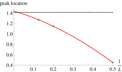
Figure 8: The peak location $g_{p}(L)$ of the best interpolating functions for $L=2,5$ and $8$ is plotted to $1/L$ (symbol). The solid line shows fitting by the ansatz $g_{p}(L)=p_{0}+p_{1}/L+p_{2}/L^{2}$ with $p_{0}=1.44004$, $p_{1}=-1.1182$ and $p_{2}=-1.71877$. The dotted line denotes “$\sqrt{2}$”, which is the phase transition point in the $L\rightarrow\infty$ limit.

On the other hand, the Padé approximant with some $(m,n)$ should be exact for finite $L$ since the exact answer is the rational function of $g$. This implies that even if we have a phase transition in discrete system in infinite volume limit, our interpolating scheme would be indirectly useful to extract information on phase transition. Indeed we have seen that the best interpolating functions precisely give the peak locations of the exact answers for finite $L$ although we need higher $(m,n)$ to correctly reproduce the values at the peaks except $L=2$. Indeed if we perform fitting of the peak locations of the best interpolating functions as a function of $L$, then we find that the peak location in the $L\rightarrow\infty$ is given by $g=1.44004$ as depicted in fig. 8. This value is fairly close to the phase transition point $g=\sqrt{2}$. We expect that this feature is true also for more general discrete systems.

4.3 Average plaquette in pure $SU(3)$ Yang-Mills theory on lattice

In this subsection, we study average plaquette in 4d pure $SU(3)$ Yang-Mills theory on lattice. Although we can compute this by preforming Monte Carlo simulation as first performed by Creutz [10], exact analytical result is unknown.

Set up

Let us consider the pure $SU(3)$ Yang-Mills theory on 4d hypercubic lattice with the standard Wilson action [11]

$$S=\beta\sum_{\mu<\nu}\sum_{\mathbf{x}}\Bigl{[}1-\frac{1}{3}{\rm ReTr}U_{\mathbf{x},\mu}U_{\mathbf{x}+\hat{\mu},\nu}U_{\mathbf{x}+\hat{\nu},\mu}^{\dagger}U_{\mathbf{x},\nu}^{\dagger}\Bigr{]},$$ (4.27)

where $U_{\mathbf{x},\mu}$ is the link variable at the position $\mathbf{x}$ with direction $\mu$ and $\hat{\mu}$ is the unit vector along $\mu$-direction. The parameter $\beta$ is related to the bare gauge coupling $g_{0}^{2}$ by $\beta=6/g_{0}^{2}$. In terms of the link variables, we introduce average plaquette by

$$P(\beta)=\Bigl{\langle}1-\frac{1}{3}{\rm Tr}U_{\mathbf{x},\mu}U_{\mathbf{x}+\hat{\mu},\nu}U_{\mathbf{x}+\hat{\nu},\mu}^{\dagger}U_{\mathbf{x},\nu}^{\dagger}\Bigr{\rangle}.$$ (4.28)

Although we can obtain numerical value of this by performing Monte Carlo simulation, there is no known analytical result of this quantity for arbitrary $\beta$. However, we have analytical result of strong coupling expansion and numerical result of weak coupling expansion with high precision on infinite lattice.

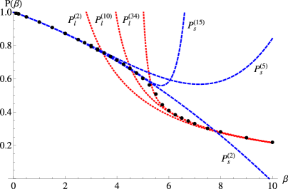
Figure 9: The average plaquette $P(\beta)$ in the 4d pure $SU(3)$ Yang-Mills theory is plotted to $\beta$.

The result of the strong coupling expansion around $\beta=0$ is given by (see e.g. [12])

$$P_{s}^{(15)}(\beta)=\sum_{k=0}^{15}s_{k}\beta^{k},$$ (4.29)

where the coefficients are explicitly given by

$$s_{0}=1,\quad s_{1}=-\frac{1}{18},\quad s_{2}=-\frac{1}{216},\quad s_{3}=0,\quad s_{4}=\frac{5}{93312},\quad s_{5}=\frac{49}{15116544},\mbox{$$}$$

$$s_{6}=-\frac{1309}{906992640},\quad s_{7}=-\frac{2131}{5441955840},\quad s_{8}=-\frac{1091}{43535646720},\mbox{$$}$$

$$s_{9}=\frac{179081}{21158324305920},\quad s_{10}=\frac{1277749}{592433080565760},\quad s_{11}=\frac{93151153}{11516899086198374400},\mbox{$$}$$

$$s_{12}=-\frac{3052831769}{34550697258595123200},\quad s_{13}=-\frac{6757393949}{414608367103141478400},\mbox{$$}$$

$$s_{14}=\frac{1932793007}{3198407403367091404800},\quad s_{15}=\frac{16029793987553}{21761963972509689918259200}.$$ (4.30)

The result of the weak coupling expansion around $\beta=\infty$ is [13] (see also [14, 15, 16, 17])

$$P_{l}^{(34)}(\beta)=\frac{1}{\beta}\sum_{k=0}^{34}l_{k}\beta^{-k},$$ (4.31)

where

$$l_{0}=2,\quad l_{1}=1.22084,\quad l_{2}=2.96043,\quad l_{3}=9.40538,\quad l_{4}=34.3245,\mbox{$$}$$

$$l_{5}=136.471,\quad l_{6}=575.197,\quad l_{7}=2528.31,\quad l_{8}=11474.2,\quad l_{9}=53450.1,\mbox{$$}$$

$$l_{10}=254138,\quad l_{11}=1.22928\times 10^{6},\quad l_{12}=6.02757\times 10^{6},\quad l_{13}=2.99220\times 10^{7},\mbox{$$}$$

$$l_{14}=1.50156\times 10^{8},\quad l_{15}=7.60422\times 10^{8},\quad l_{16}=3.88155\times 10^{9},\mbox{$$}$$

$$l_{17}=1.99751\times 10^{10},\quad l_{18}=1.03474\times 10^{11},\quad l_{19}=5.38793\times 10^{11},\mbox{$$}$$

$$l_{20}=2.82781\times 10^{12},\quad l_{21}=1.4928\times 10^{13},\quad l_{22}=7.94067\times 10^{13},\mbox{$$}$$

$$l_{23}=4.25644\times 10^{14},\quad l_{24}=2.30516\times 10^{15},\quad l_{25}=1.26685\times 10^{16},\mbox{$$}$$

$$l_{26}=7.12124\times 10^{16},\quad l_{27}=4.13752\times 10^{17},\quad l_{28}=2.5183\times 10^{18},\mbox{$$}$$

$$l_{29}=1.63433\times 10^{19},\quad l_{30}=1.15935\times 10^{20},\quad l_{31}=8.72907\times 10^{20},\mbox{$$}$$

$$l_{32}=6.86167\times 10^{21},\quad l_{33}=5.82436\times 10^{22},\quad l_{34}=5.09837\times 10^{23}.$$ (4.32)

The plot in fig. 9 shows the result of our Monte Carlo simulation on $10^{4}$ lattice, $P_{s}^{(N_{s})}(\beta)$ and $P_{l}^{(N_{l})}(\beta)$ (for some values of $N_{s}$ and $N_{l}$) against $\beta$. Now we determine the parameters $\beta_{s}^{\ast}$, $N_{s}^{\ast}$, $\beta_{l}^{\ast}$ and $N_{l}^{\ast}$.

Determination of $\beta_{s}^{\ast}$

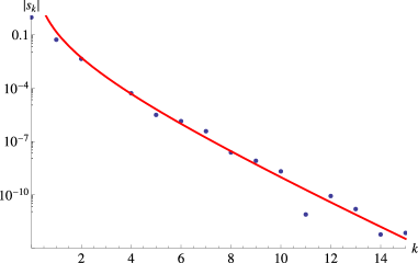
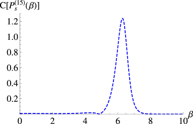
Figure 10: [Left] The absolute value of the $k$-th coefficient of the strong coupling expansion is plotted against $k$ in semi-log scale. The solid line shows the fitting function $\log{|s_{k}|}=\log{c_{s}}+a_{s}\log{k}+k\log{A_{s}}$. [Right] The absolute value of the curvature of $P_{s}^{(15)}(\beta)$ is plotted to $\beta$.

Let us study large order behavior of the strong coupling expansion. In fig. 10 [Left], we plot $|s_{k}|$ against $k$ in semi-log scale. By fitting this by the ansatz

$$|s_{k}|=c_{s}k^{a_{s}}A_{s}^{k},$$ (4.33)

we obtain

$$c_{s}=0.576352,\quad a_{s}=-2.82846,\quad A_{s}=0.254563.$$ (4.34)

This implies that the strong coupling expansion is convergent inside the circle $|\beta|\sim A_{s}^{-1}=3.9283$. We also plot the curvature of $P_{s}^{(15)}$ to $\beta$ in fig. 10 [Right] in order to find blow-up point. Then we find that $P_{s}^{(15)}$ blows up at $\beta=\beta_{s}^{b}=6.28417$. Thus we take the values of $N_{s}^{\ast}$ and $\beta_{s}^{\ast}$ as

$$N_{s}^{\ast}=15,\quad\beta_{s}^{\ast}=3.9.$$ (4.35)

Determination of $\beta_{l}^{\ast}$

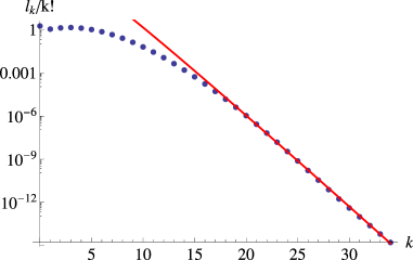
Figure 11: The weak coupling expansion coefficient $l_{k}$ divided by $k!$ is plotted to $k$ in semi-log scale. The line denotes fitting by the function $\log{(l_{k}/k!)}=\log{c_{l}}+a_{l}\log{k}+k\log{A_{l}}$.

Next we study large order behavior of the weak coupling expansion. Fig. 11 plots $l_{k}/k!$ against $k$ in semi-log scale. From this plot we find that the coefficient in large $k$ regime grows as

$$\frac{l_{k}}{k!}\sim c_{l}k^{a_{l}}A_{l}^{k},\quad{\rm with}\ c_{l}=0.0000946747,\ a_{l}=11.1583\ {\rm and}\ A_{l}=0.14984.$$ (4.36)

This exhibits that the coefficient grows by the factorial and hence the weak coupling expansion is asymptotic. By performing optimization, we find

$$N_{l}^{o}=\frac{\beta}{A_{l}},\quad\delta_{l}(\beta)=c_{l}\left(\frac{\beta}{A_{l}}+1\right)^{a_{l}}e^{-\frac{\beta}{A_{l}}}.$$ (4.37)

If we take $\epsilon_{l}=10^{-4}$, then we should take $N_{l}^{o}=40$ and $\beta_{l}^{\ast}=5.99358$. However, since we know the only first 35 coefficients of the weak coupling expansion, we cannot perform this optimization and instead we demand

$$\left.\left(c_{l}k^{a_{w}}A_{l}^{k}(\beta_{l}^{\ast})^{-1-k}\right)\right|_{k=35}=\epsilon_{l}.$$ (4.38)

Thus we take

$$N_{l}^{\ast}=34,\quad\beta_{l}^{\ast}=6.13706.$$ (4.39)

Result

	$\frac{1}{29}\sum_{i}\bigl{|}\frac{P_{m,n}^{(\alpha)}-P}{P}\bigr{|}$	$I_{s}[P_{m,n}^{(\alpha)}]$	$I_{l}[P_{m,n}^{(\alpha)}]$	$I_{s}+I_{l}$
$P_{1,1}^{(-1)}$	0.228616	0.634296	0.222215	0.856510
$P_{1,1}^{(-1/3)}$	0.115055	0.206451	0.070088	0.276539
$P_{2,2}^{(-1)}$	0.158456	0.380170	0.0924484	0.472619
$P_{3,3}^{(-1)}$	0.119927	0.247194	0.0472852	0.294479
$P_{4,4}^{(-1)}$	0.0956988	0.168693	0.0272632	0.195956
$P_{5,5}^{(-1)}$	0.0790835	0.118552	0.0169992	0.135551
$P_{6,6}^{(-1)}$	0.0670207	0.0848353	0.0112119	0.0960472
$P_{7,7}^{(-1)}$	0.0579211	0.0614099	0.00772215	0.0691320
$P_{8,8}^{(-1)}$	0.0508609	0.0447886	0.00550651	0.0502934
$P_{9,9}^{(-1)}$	0.0452512	0.0328091	0.00403859	0.0368477
$P_{10,10}^{(-1)}$	0.0406960	0.0240752	0.00303056	0.0271057
$P_{11,11}^{(-1)}$	0.0369267	0.0176544	0.00231792	0.0199723
$P_{12,12}^{(-1)}$	0.0337611	0.0129187	0.00180261	0.0147214
$P_{13,13}^{(-1)}$	0.0310727	0.00942950	0.00142323	0.0108527
$P_{14,14}^{(-1)}$	0.0287673	0.00686572	0.00113935	0.00800507
$\bf P_{15,15}^{(-1)}$	$\bf 0.0267697$	$\bf 0.00498586$	$\bf 0.000923484$	$\bf 0.00590935$

Table 6: Result on the 4d $SU(3)$ pure Yang-Mills theory on lattice.

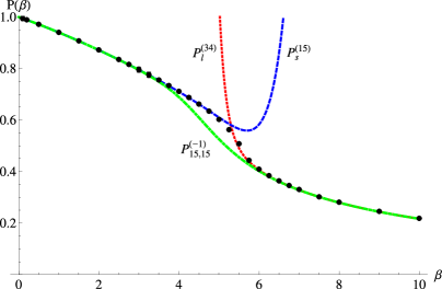
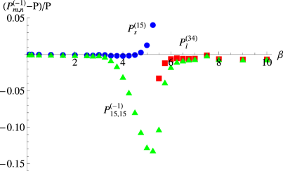
Figure 12: [Left] The best interpolating function $P_{15,15}^{(-1)}(\beta)$ (green dot-dashed), the strong coupling expansion $P_{s}^{(15)}(\beta)$ (blue dashed) and the weak coupling expansion $P_{l}^{(34)}(\beta)$ (red dotted) are plotted to $\beta$ with the Monte Carlo simulation result (symbol). [Right] The ratios $(P_{15,15}^{(-1)}(\beta)-P(\beta))/P(\beta)$ (green triangle), $(P_{s}^{(15)}(\beta)-P(\beta))/P(\beta)$ (blue circle) and $(P_{l}^{(34)}(\beta)-P(\beta))/P(\beta)$ (red square) are plotted against $\beta$. Here $P(\beta)$ means the Monte Carlo result.

Let us test our criterion in this example. In terms of the strong and weak coupling expansions, we can construct interpolating functions $P_{m,n}^{(\alpha)}(\beta)$ of the average plaquette $P(\beta)$ taking the FPR form (2.7). Since we do not know exact analytical result for the plaquette, we measure precision of approximation in terms of the Monte Carlo result by using

$$\frac{1}{29}\sum_{i=1}^{29}\left|\frac{P_{m,n}^{(\alpha)}(\beta_{i})-P(\beta_{i})}{P(\beta_{i})}\right|.$$ (4.40)

This quantity should be minimized by the best interpolating function. Compared with values of $I_{s}[P_{m,n}^{(\alpha)}]$ and $I_{l}[P_{m,n}^{(\alpha)}]$, we test validity of our criterion. We summarize our result in tab. 6. Explicit formula for the interpolating functions can be found in app. B.3. We easily see that the interpolating function $P_{15,15}^{(-1)}(\beta)$ gives the most precise approximation of $P(\beta)$, which minimizes $I_{s}$ and $I_{l}$ among the interpolating functions. This shows that our criterion correctly chooses the best interpolating function for this case. We also plot the best interpolating function $P_{15,15}^{(-1)}(\beta)$ and its normalized difference from the Monte Carlo result in fig. 12. We find that $P_{15,15}^{(-1)}(\beta)$ approximates the average plaquette with about $13\%$ error at worst. Because finding interpolating functions becomes so heavy for larger $m+n$, we have stopped this up to $m+n=30$. It is interesting if we use our full knowledge about the weak and strong coupling expansions to construct better interpolating functions.

4.4 Free energy in $c=1$ string theory at self-dual radius

Let us consider so-called $c=1$ string theory at self-dual radius (for excellent reviews, see [20, 21, 22]). The free energy in the $c=1$ string theory has the following integral representation [23, 24, 25]

$$\tilde{F}(\mu)=\frac{\mu^{2}}{2}\log{\mu}-\frac{1}{12}\log{\mu}+\frac{1}{4}\int_{0}^{\infty}\frac{ds}{s}\left(\frac{1}{\sinh^{2}{s}}-\frac{1}{s^{2}}+\frac{1}{3}\right)e^{-2\mu s},$$ (4.41)

where $\mu$ is the cosmological constant related to the string coupling constant $g_{s}$ roughly by $\mu\sim g_{s}^{-1}$. This behavior can be also seen in critical behavior of topological string at the conifold point [26]. Beside the contexts of string theory, the last term in the above equation has also an interpretation from Schwinger effect [27, 28] as noted in [25].

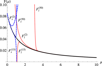
Figure 13: The free energy $F(\mu)$ in the $c=1$ string theory at self-dual radius is plotted to $\mu$.

We can perform large $\mu$ and small $\mu$ expansions of $\tilde{F}(\mu)$. The large $\mu$ expansion, which we call weak coupling expansion, is given by

$$\tilde{F}(\mu)=\frac{\mu^{2}}{2}\log{\mu}-\frac{1}{12}\log{\mu}-\sum_{p\geq 2}\frac{B_{2p}}{2p(2p-2)}\mu^{2-2p},$$ (4.42)

while the small $\mu$ expansion, which we refer to as strong coupling expansion, is given by

$$\tilde{F}(\mu)=\mu^{2}\log{\mu}-\frac{1}{6}\log{\mu}+\frac{1}{12}-\log{A}+2\mu+\mu^{2}(-1+2\gamma)+\sum_{p\geq 3}\frac{(-\mu)^{p}}{p}\zeta(p-1).$$ (4.43)

Here $A$ and $\gamma$ are Glaisher constant and Euler constant, respectively. Since the two expansions of $\tilde{F}(\mu)$ do not take the power series forms, we redefine the free energy as

$$F(\mu)=\tilde{F}(\mu)-\left(\frac{\mu^{2}}{2}-\frac{1}{12}\right)\log{\mu}+\left(\frac{\mu^{2}}{2}-\frac{1}{12}\right)\log{\frac{\mu+1}{\mu}}-\frac{\mu}{2}+\frac{1}{4}.$$ (4.44)

Then we find that $F(\mu)$ has the following two power series expansions

$$F(\mu) = \left(\frac{1}{3}-\log{A}\right)-\frac{\mu}{12}+\left(\frac{\gamma}{2}-\frac{5}{24}\right)\mu^{2}+\left(\frac{17}{36}-\frac{\pi^{2}}{18}\right)\mu^{3}+\left(\frac{\zeta(3)}{4}-\frac{11}{48}\right)\mu^{4}+\mathcal{O}\left(\mu^{5}\right)\mbox{$$}$$ (4.45)

$$= \mu^{-1}\left(\frac{1}{12}-\frac{19}{240}\mu^{-1}+\frac{13}{180}\mu^{-2}-\frac{4}{63}\mu^{-3}+\frac{23}{420}\mu^{-4}+\mathcal{O}\left(\mu^{-5}\right)\right).$$

Let us call the above two expansions $F_{s}^{(N_{s})}(\mu)$ (up to $\mathcal{O}(\mu^{N_{s}})$) and $F_{l}^{(N_{l})}(\mu)$ (up to $\mathcal{O}(\mu^{-1-N_{l}})$):

$$F_{s}^{(N_{s})}(\mu)=\sum_{k=0}^{N_{s}}s_{k}\mu^{k},\quad F_{l}^{(N_{l})}(\mu)=\mu^{-1}\sum_{k=0}^{N_{l}}l_{k}\mu^{-k}.$$ (4.46)

We assume again that we have information only on $F_{s}^{(50)}(\mu)$ and $F_{l}^{(50)}(\mu)$, and read large order behaviors of $s_{k}$ and $l_{k}$ by extrapolation. In fig. 13, we plot the result of numerical integration, $F_{s}^{(N_{s})}(\mu)$ and $F_{l}^{(N_{l})}(\mu)$ ($N_{s},N_{l}=2,15,50$) against $\mu$.

Determination of $\mu_{s}^{\ast}$

By fitting the data of $s_{k}$ for $k=15\sim 50$, we find

$$|s_{k}|\sim c_{s}k^{a_{s}},\quad{\rm with}\ c_{s}=0.415148\ {\rm and}\ a_{s}=-0.920281.$$ (4.47)

Thus we expect that the strong coupling expansion is convergent for $|\mu|<1$. We also find a blow-up point of $F_{s}^{(50)}(\mu)$ around $\mu=1.01862$ and hence take

$$N_{s}^{\ast}=50,\quad\mu_{s}^{\ast}=0.8.$$ (4.48)

Determination of $\mu_{l}^{\ast}$

Fitting the data of $l_{k}$ for $k=10\sim 50$ shows

$$\frac{|l_{2k+1}|}{(2k)!}\sim c_{l}A_{l}^{k},\quad{\rm with}\ c_{l}=0.220021\ {\rm and}\ A_{l}=0.0284273.$$ (4.49)

Thus the weak coupling expansion is asymptotic and its optimization leads us to

$$N_{l}^{o}=\frac{\mu}{\sqrt{A_{l}}}+1,\quad\delta_{l}(\mu)=\frac{c_{l}}{\mu}e^{-\frac{\mu}{\sqrt{A_{l}}}}.$$ (4.50)

Taking $\epsilon_{l}=10^{-9}$, we find

$$N_{l}^{o}=N_{l}^{\ast}=21,\quad\mu_{l}^{\ast}=3.37208.$$ (4.51)

Result

	$\frac{1}{199}\sum_{i}\bigl{|}\frac{F_{m,n}^{(\alpha)}-F}{F}\bigr{|}$	$I_{s}[F_{m,n}^{(\alpha)}]$	$I_{l}[F_{m,n}^{(\alpha)}]$	$I_{s}+I_{l}$
$F_{1,1}^{(-1)}$	0.000136491	$6.53166\times 10^{-6}$	$9.73821\times 10^{-6}$	0.0000162699
$F_{1,1}^{(-1/3)}$	0.0000731361	$2.70362\times 10^{-6}$	$5.61321\times 10^{-6}$	$8.31684\times 10^{-6}$
$F_{2,2}^{(-1)}$	$4.19545\times 10^{-6}$	$1.51251\times 10^{-7}$	$2.44485\times 10^{-7}$	$3.95735\times 10^{-7}$
$F_{2,2}^{(-1/3)}$	0.0000238415	$8.52636\times 10^{-7}$	$1.46650\times 10^{-6}$	$2.31914\times 10^{-6}$
$F_{2,2}^{(-1/5)}$	$6.3568\times 10^{-6}$	$5.54772\times 10^{-7}$	$2.10621\times 10^{-7}$	$7.65393\times 10^{-7}$
$F_{3,3}^{(-1)}$	$2.68298\times 10^{-7}$	$8.50196\times 10^{-9}$	$1.36795\times 10^{-8}$	$2.21815\times 10^{-8}$
$F_{3,3}^{(-1/3)}$	$3.80959\times 10^{-7}$	$1.86495\times 10^{-8}$	$1.30998\times 10^{-8}$	$3.17493\times 10^{-8}$
$F_{3,3}^{(-1/7)}$	$1.50436\times 10^{-6}$	$9.96742\times 10^{-8}$	$4.56374\times 10^{-8}$	$1.45312\times 10^{-7}$
$F_{4,4}^{(-1)}$	$5.60104\times 10^{-9}$	$1.19446\times 10^{-9}$	$1.25679\times 10^{-10}$	$1.32014\times 10^{-9}$
$F_{4,4}^{(-1/3)}$	$5.48471\times 10^{-8}$	$2.58923\times 10^{-9}$	$1.67657\times 10^{-9}$	$4.26580\times 10^{-9}$
$F_{4,4}^{(-1/9)}$	$4.17108\times 10^{-8}$	$2.65563\times 10^{-9}$	$1.88948\times 10^{-9}$	$4.54512\times 10^{-9}$
$\bf F_{5,5}^{(-1)}$	$\bf 5.40195\times 10^{-9}$	$\bf 1.18856\times 10^{-9}$	$\bf 1.20303\times 10^{-10}$	$\bf 1.30886\times 10^{-9}$
$F_{5,5}^{(-1/11)}$	$6.11560\times 10^{-8}$	$6.08949\times 10^{-9}$	$7.90103\times 10^{-10}$	$6.87959\times 10^{-9}$

Table 7: Result on the $c=1$ string theory at self-dual radius

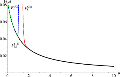
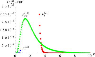
Figure 14: [Left] The best interpolating function $F_{5,5}^{(-1)}(\mu)$ (green dot-dashed), the strong coupling expansion $F_{s}^{(50)}(\mu)$ (blue dashed) and the weak coupling expansion $F_{l}^{(21)}(\mu)$ (red dotted) are plotted to $\mu$ with the result of numerical integration (symbol). Note that $F_{5,5}^{(-1)}(\mu)$ is almost the numerical integration result. [Right] The ratios $(F_{5,5}^{(-1)}(\mu)-F(\mu))/F(\mu)$ (green triangle), $(F_{s}^{(50)}(\mu)-F(\mu))/F(\mu)$ (blue circle) and $(F_{l}^{(21)}(\mu)-F(\mu))/F(\mu)$ (red square) are plotted against $\mu$. Here $F(\mu)$ means the result of the numerical integration.

Let us check our criterion in this example. We can construct interpolating functions $F_{m,n}^{(\alpha)}(\mu)$ of $F(\mu)$ in terms of the two expansions (see appendix B.4 for explicit formula). We measure precision of approximation in terms of the numerical integration result $F(\mu_{i})$ by

$$\frac{1}{199}\sum_{i=1}^{199}\left|\frac{F_{m,n}^{(\alpha)}(\mu_{i})-F(\mu_{i})}{F(\mu_{i})}\right|,$$ (4.52)

where $\mu_{i}=i/200$. Comparing this with values of $I_{s}[F_{m,n}^{(\alpha)}]$ and $I_{l}[F_{m,n}^{(\alpha)}]$, we can test our criterion as in the other examples. We summarize our result in tab. 7. We easily see that the interpolating function $F_{5,5}^{(-1)}(\mu)$ gives the most precise approximation of $F(\mu)$, which minimizes $I_{s}$ and $I_{l}$ among the candidates. This shows that our criterion correctly chooses the best interpolating function for this example. We also plot the best interpolating function $F_{5,5}^{(-1)}(\beta)$ and its normalized difference from the numerical integration result in fig. 14. We also observe that the best interpolating function gives the very precise approximation.

5 Discussions

In this paper we have studied interpolating function, which is smooth and consistent with two perturbative expansions of physical quantity around different two points. First we have proposed the new type of interpolating function, which is described by fractional power of rational function, and includes the Padé approximant and FPP constructed by Sen [1] as the special cases. After introducing the interpolating functions, we have pointed out that we can construct enormous number of such interpolating functions in principle while the “best” approximation of the exact answer should be unique among the interpolating functions. Then we have proposed the criterion (3.2) to determine the “best” interpolating function without knowing the exact answer of the physical quantity. This criterion depends on convergence properties of the small-$g$ and large-$g$ expansions. We have explicitly checked that our criterion works for various examples including the specific heat in the 2d Ising model, the average plaquette in the 4d $SU(3)$ pure Yang-Mills theory on lattice and free energy in the $c=1$ string theory at self-dual radius. We expect that our criterion is applicable unless a problem of interest does not have mixed non-perturbative effect, which is non-perturbative in the both senses of the small-$g$ and large-$g$ expansions.

Besides cases with mixed non-perturbative effects, we have also found another limitation of approximation by our interpolating function. In the 2d Ising model on infinite lattice, we have observed that interpolating functions do not correctly describe the phase transition although our criterion correctly chooses the relatively best approximation. This is obvious since our interpolating functions are smooth by construction unless they have poles. This indicates that our interpolating scheme cannot be directly used for approximation when we have a phase transition. On the other hand, we have seen that our best interpolating functions precisely give the peak locations of the exact answers for finite lattice size $L$, which converges to the phase transition point in the $L\rightarrow\infty$ limit. Indeed fitting the peak locations as the function of $L$ leads the peak location in the $L\rightarrow\infty$ limit, which is very close to the phase transition point. This implies that even if we have a phase transition in discrete system in infinite volume limit, our interpolating scheme would be indirectly useful to extract information on phase transition. We expect that this feature is true also for more general discrete systems.

One of obvious possible applications of our work is to apply our interpolating scheme to physical quantities in diverse physical systems. Although we have worked on the examples in this paper, where we know the exact answers or numerical results for the whole regions, we can study more nontrivial system by using our criterion. We expect that our results are useful in various context of theoretical physics.

In this paper, we have focused on how to choose the relatively best interpolating functions among candidates in fixed problems. Conversely, it is also interesting to classify problems, which is approximated very well by the FPR (2.7) with each fixed $\alpha$.

Although our criterion works in the various examples, our criterion might be too naive, need slight modifications or have some other exceptions. It is very illuminating if we can perform more rigorous treatment and precisely find necessary or sufficient conditions for validity of our criterion.

Also, our criterion requires information on large order behaviors of perturbative expansions. From more practical point of view, it is very nice if there exists an alternative equivalent criterion, which uses fewer information on the expansions.

We close by mentioning possible relation to recent progress on resurgence in quantum field theory [29, 30, 31, 32, 33, 34, 35, 36, 37, 38, 39] (see also recent Borel analysis [40, 41, 42, 43, 44] in extended supersymmetric field theories). While ordinary weak coupling expansion (namely the one around trivial saddle point) generically has non-perturbative ambiguity, we expect that the ambiguity is partially fixed by interpolation to strong coupling expansion as far as we focus on real positive coupling at least. Also our interpolating scheme seems to have no obstruction even if perturbative expansions are non-Borel summable. It is interesting to study interpolation problem in theories concerned with resurgence and make clear such a relation.

Acknowledgment

We are grateful to Ashoke Sen and Tomohisa Takimi for their early collaborations, many valuable discussions and reading the manuscript. We thank Sinya Aoki and Yuji Tachikawa for careful reading manuscript and many useful comments.

Appendix A Analysis of two-dimensional Ising model by another parameter

In sec. 4.2, we have analyzed the interpolation problem in the 2d Ising model by using the parameter $e^{2K}=1+g$. Then we have seen that the exact solution of the quantity $C_{L}(g)$ is the rational function of $g$ for finite $L$ and hence one of the Padé approximants gives the exact solution. It would be interesting to repeat this analysis in terms of another parameter choice, where all the FPR interpolating function (2.7) do not give the exact solution.

In this appendix, we repeat a part of analysis in section 4.2 by using the parameter

$$e^{8K}=1+g^{2}.$$ (A.1)

Then the exact solution of $C_{L}(g)$ with finite $L$ becomes a rational function of $\sqrt{1+g^{2}}$, which does not take the form (2.7) of FPR at least for $L=5$ and $L=8$. Here we do not explicitly write down formulas of interpolating functions but we have uploaded a Mathematica file to arXiv, which writes down the explicit forms.

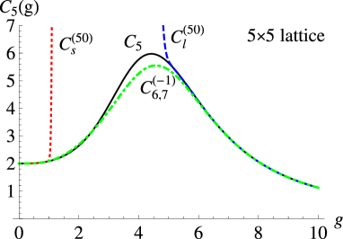
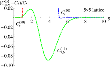
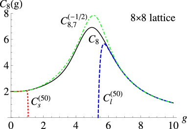
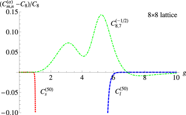
Figure 15: [Left] The function $C_{L}(g)$ (black solid), the best interpolating function (green dot-dashed), its high (red dotted) and low (blue dashed) temperature expansions are plotted to $g$ for each $L$. [Right] $|(C_{m,n}^{(\alpha)}-C_{L})/C_{L}|$ (green dot-dashed), $|(C_{s}^{(50)}-C_{L})/C_{L}|$ (red dotted) and $|(C_{l}^{(50)}-C_{L})/C_{L}|$ (blue dashed) are plotted against $g$ for each $L$.

A.1 $5\times 5$ lattice

The function $C_{5}(g)$ has the expansions

$$C_{5}(g) = 2+\frac{5g^{4}}{32}+\mathcal{O}\left(g^{5}\right)\mbox{$$}$$ (A.2)

$$= g^{-2}\left(64+288g^{-1}+1088g^{-2}+4688g^{-3}+31936g^{-4}+\mathcal{O}(g^{-5})\right).$$

As in section 4.2, we find that the coefficient of the expansions grow as

$$|s_{2k}|\sim c_{s}A_{s}^{k},\quad {\rm with}\ c_{s}=0.139016\ {\rm and}\ A_{s}=0.983446,\mbox{$$}$$

$$|l_{k}|\sim c_{l}A_{l}^{k},\quad {\rm with}\ c_{l}=149.71\ {\rm and}\ A_{l}=4.76806,$$ (A.3)

and the blow-up points are $g_{s}^{b}=0.972788$ and $g_{l}^{b}=5.02376$. Thus we take

$$N_{s}^{\ast}=50,\quad g_{s}^{\ast}=0.8,\quad N_{l}^{\ast}=50,\quad g_{l}^{\ast}=5.5.$$ (A.4)

Our result is summarized in fig. 15 and tab. 8. We see that the best interpolating function $C_{6,7}^{(-1)}$ minimizes $I_{s}+I_{l}$.

	$\Lambda^{-1}\int dg\bigl{|}\frac{C_{m,n}^{(\alpha)}-C_{5}}{C_{5}}\bigr{|}$	$I_{s}[C_{m,n}^{(\alpha)}]$	$I_{l}[C_{m,n}^{(\alpha)}]$	$I_{s}+I_{l}$
$C_{1,1}^{(-2)}$	0.0144367	0.0213492	10.3506	10.3719
$C_{1,1}^{(-2/3)}$	0.00356604	0.00230782	4.09192	4.09423
$C_{1,2}^{(-1/2)}$	0.00449818	0.0109249	5.46089	5.47181
$C_{2,2}^{(-2)}$	0.00796436	0.00837338	8.29550	8.30388
$C_{2,3}^{(-1)}$	0.00272780	0.00432520	3.09134	3.09567
$C_{2,3}^{(-1/2)}$	0.00397428	0.00752549	4.80614	4.81367
$C_{2,3}^{(-1/3)}$	0.00275912	0.00696200	2.67071	2.67767
$C_{3,2}^{(-1)}$	0.00633731	0.00740158	7.17559	7.18299
$C_{3,2}^{(-1/2)}$	0.00375206	0.00722903	4.51172	4.51895
$C_{3,2}^{(-1/3)}$	0.00500575	0.00740608	6.16320	6.17060
$C_{3,3}^{(-2)}$	0.00594014	0.00740588	7.03028	7.03768
$C_{3,4}^{(-1/2)}$	0.00378784	0.00723170	4.55132	4.55855
$C_{3,4}^{(-1/3)}$	0.00277366	0.00701077	2.72476	2.73177
$C_{3,4}^{(-1/4)}$	0.00311106	0.00735004	3.34761	3.35496
$C_{4,3}^{(-1)}$	0.00285537	0.00512428	3.24096	3.24608
$C_{4,3}^{(-1/2)}$	0.00397491	0.00754047	4.80695	4.81449
$C_{4,3}^{(-1/3)}$	0.00276431	0.00698137	2.69046	2.69744
$C_{4,5}^{(-1/2)}$	0.00257637	0.00641159	2.49159	2.49800
$C_{4,5}^{(-1/3)}$	0.00276420	0.00698123	2.68889	2.69587
$C_{4,5}^{(-1/4)}$	0.00324266	0.00741956	3.81888	3.82630
$C_{5,4}^{(-1/3)}$	0.00277377	0.00701331	2.72502	2.73203
$C_{5,6}^{(-1/2)}$	0.00198535	0.00470116	1.35410	1.35880
$\bf C_{6,7}^{(-1)}$	$\bf 0.000206236$	$\bf 0.000285621$	$\bf 0.0530750$	$\bf 0.0533606$
$C_{6,7}^{(-1/4)}$	0.00370596	0.00206143	4.90389	4.90595
$C_{7,8}^{(-1/2)}$	0.00155076	0.000172986	1.10463	1.10480
$C_{8,7}^{(-1)}$	0.00116219	0.0000226883	1.07748	1.07750
$C_{8,9}^{(-1)}$	0.000667177	0.0000119276	0.353759	0.353771
$C_{8,9}^{(-1/3)}$	0.00175529	0.0000171883	2.16789	2.16791
$C_{9,8}^{(-1)}$	0.000932892	0.0000183826	0.719767	0.719786
$C_{9,8}^{(-1/2)}$	0.00157844	0.0000190668	3.13313	3.13315
$C_{9,8}^{(-1/3)}$	0.00210168	0.0000232122	2.63069	2.63071

Table 8: Result for $L=5$

	$\Lambda^{-1}\int dg\bigl{|}\frac{C_{m,n}^{(\alpha)}-C_{8}}{C_{8}}\bigr{|}$	$I_{s}[C_{m,n}^{(\alpha)}]$	$I_{l}[C_{m,n}^{(\alpha)}]$	$I_{s}+I_{l}$
$C_{1,1}^{(-2)}$	0.0143447	0.0210712	8.19673	8.21780
$C_{1,1}^{(-2/3)}$	0.00358516	0.00215995	2.97922	2.98138
$C_{1,2}^{(-1/2)}$	0.00445291	0.0106469	3.94941	3.96005
$C_{2,1}^{(-1)}$	0.00984413	0.00828929	6.80598	6.81427
$C_{2,1}^{(-1/2)}$	0.00486112	0.00620801	2.61762	2.62382
$C_{2,2}^{(-2)}$	0.00787515	0.00809537	6.39885	6.40694
$C_{2,2}^{(-2/5)}$	0.00452636	0.00760081	4.06211	4.06971
$C_{2,3}^{(-1)}$	0.00289778	0.00419641	2.55162	2.55581
$C_{2,3}^{(-1/2)}$	0.00402696	0.00742413	3.52709	3.53451
$C_{2,3}^{(-1/3)}$	0.00297962	0.00671530	1.98072	1.98743
$C_{3,2}^{(-1)}$	0.00625943	0.00712357	5.44665	5.45377
$C_{3,2}^{(-1/2)}$	0.00372974	0.00695102	3.20299	3.20994
$C_{3,3}^{(-2)}$	0.00587186	0.00712823	5.31167	5.31880
$C_{3,4}^{(-1/2)}$	0.00379867	0.00695734	3.27471	3.28167
$C_{3,4}^{(-1/3)}$	0.00341859	0.00701707	2.73224	2.73926
$C_{3,4}^{(-1/4)}$	0.00369312	0.00708313	3.17778	3.18486
$C_{4,3}^{(-1)}$	0.00300812	0.00492987	2.63094	2.63587
$C_{4,3}^{(-1/2)}$	0.00402822	0.00746425	3.52822	3.53568
$C_{4,3}^{(-1/3)}$	0.00298748	0.00673209	1.99653	2.00326
$C_{4,5}^{(-1/2)}$	0.00293553	0.00614008	2.16315	2.16929
$C_{4,5}^{(-1/3)}$	0.00345399	0.00715123	2.78100	2.78815
$C_{4,5}^{(-1/4)}$	0.00317186	0.00694968	2.32397	2.33091
$C_{5,4}^{(-1/3)}$	0.00351452	0.00837605	2.85851	2.86688
$C_{5,6}^{(-1/4)}$	0.00327626	0.00722693	2.49615	2.50337
$C_{6,5}^{(-1/2)}$	0.000875711	0.000194793	0.595842	0.596037
$C_{6,5}^{(-1/3)}$	0.00344271	0.00621808	2.77138	2.77760
$C_{6,7}^{(-1/3)}$	0.00109210	0.0000803322	0.348460	0.348541
$C_{6,7}^{(-1/4)}$	0.00323839	0.00629399	2.44618	2.45247
$C_{7,8}^{(-1/3)}$	0.00155789	0.0000565836	0.762480	0.762537
$\bf C_{8,7}^{(-1/2)}$	$\bf 0.000350404$	$\bf 0.0000254784$	$\bf 0.0719374$	$\bf 0.0719629$
$C_{8,7}^{(-1/3)}$	0.00120052	0.0000117739	0.411958	0.411969
$C_{9,8}^{(-1/3)}$	0.000896865	$1.25557\times 10^{-6}$	0.148141	0.148142

Table 9: Result for $L=8$

A.2 $8\times 8$ lattice

The high and low temperature expansions of $C_{8}(g)$ are given by

$$C_{8}(g) = 2+\frac{5g^{4}}{32}+\mathcal{O}\left(g^{5}\right)\mbox{$$}$$ (A.5)

$$= g^{-2}\left(64+288g^{-1}+1088g^{-2}+4688g^{-3}+19264g^{-4}+\mathcal{O}(g^{-5})\right).$$

As in the $L=5$ case , we find

$$c_{s}=0.0614108,\quad A_{s}=1.04269,\quad g_{s}^{b}=0.979314,\mbox{$$}$$

$$c_{l}=99.216,\quad A_{l}=5.4084,\quad g_{l}^{b}=5.73095.$$ (A.6)

Thus we take

$$N_{s}^{\ast}=50,\quad g_{s}^{\ast}=0.8,\quad N_{l}^{\ast}=50,\quad g_{l}^{\ast}=6.3.$$ (A.7)

From tab. 9, we find that the best interpolating function $C_{8,7}^{(-1/2)}$ minimizes $I_{s}+I_{l}$.

Appendix B Explicit formula for interpolating functions

In this appendix, we explicitly write down the interpolating functions appearing in the main text. Although we often display numerical values in 6 digits, indeed we have worked on “MachinePrecision” or 100 digits in Mathematica. We have uploaded the Mathematica file to arXiv, which writes all interpolating functions in actual precisions.

B.1 Zero-dimensional $\varphi^{4}$ theory

$$\scriptscriptstyle F_{0,0}^{(1/2)}(g)=\sqrt{2\pi}\left(\frac{8\pi g}{\Gamma\left(1/4\right)^{2}}+1\right)^{-1/2},\quad F_{1,1}^{(1/2)}(g)=\sqrt{2\pi\Gamma\left(1/4\right)}\left(\frac{8\pi g\Gamma\left(1/4\right)+\Gamma\left(1/4\right)^{3}+2\pi\Gamma\left(-1/4\right)}{64\pi^{2}g^{2}+8\pi g\Gamma\left(1/4\right)^{2}+\Gamma\left(1/4\right)^{4}+2\pi\Gamma\left(-1/4\right)\Gamma\left(1/4\right)}\right)^{1/2},\mbox{$$}$$

$$\scriptscriptstyle F_{1,1}^{(1/6)}(g)=2.50663\left(\frac{1}{6.98929g^{3}+7.08691g^{2}+1}\right)^{1/6},\quad F_{2,2}^{(1/2)}(g)=2.50663\sqrt{\frac{37.9117g^{2}+10.1532g+1}{72.4854g^{3}+43.9117g^{2}+10.1532g+1}},\mbox{$$}$$

$$\scriptscriptstyle F_{2,2}^{(1/10)}(g)=2.50663\left(25.5499g^{5}+43.1779g^{4}+32.1482g^{3}+30g^{2}+1\right)^{-1/10},\mbox{$$}$$

$$\scriptscriptstyle F_{3,3}^{(1/2)}(g)=2.50663\sqrt{\frac{324.019g^{3}+110.261g^{2}+16.0304g+1}{619.509g^{4}+420.201g^{3}+116.261g^{2}+16.0304g+1}},\mbox{$$}$$

$$\scriptscriptstyle F_{3,3}^{(1/6)}(g)=2.50663\left(\frac{28.2525g^{2}+8.0997g+1}{197.465g^{5}+256.834g^{4}+145.795g^{3}+46.2525g^{2}+8.0997g+1}\right)^{1/6},\mbox{$$}$$

$$\scriptscriptstyle F_{3,3}^{(1/14)}(g)=2.50663\left(93.3994g^{7}+220.976g^{6}+239.216g^{5}+155.758g^{4}+42g^{2}+1\right)^{-1/14},\mbox{$$}$$

$$\scriptscriptstyle F_{4,4}^{(1/2)}(g)=2.50663\sqrt{\frac{3224.56g^{4}+1303.49g^{3}+238.239g^{2}+22.8745g+1}{6165.22g^{5}+4576.g^{4}+1440.74g^{3}+244.239g^{2}+22.8745g+1}},\mbox{$$}$$

$$\scriptscriptstyle F_{4,4}^{(1/10)}(g)=2.50663\left[\frac{14.4369g^{2}+5.07251g+1}{368.86g^{7}+752.954g^{6}+708.689g^{5}+403.106g^{4}+152.175g^{3}+44.4369g^{2}+5.07251g+1}\right]^{1/10},\mbox{$$}$$

$$\scriptscriptstyle F_{4,4}^{(1/18)}(g)=2.50663\left(341.428g^{9}+1038.59g^{8}+1475.35g^{7}+1294.34g^{6}+780.788g^{5}+594g^{4}+54g^{2}+1\right)^{-1/18}.$$ (B.1)

B.2 Two-dimensional Ising model

B.2.1 $2\times 2$ lattice

$$\scriptscriptstyle C_{1,1}^{(-4)}(g)=\frac{48\left(-\sqrt[4]{2}g-2\sqrt[4]{3}+\sqrt[4]{2}\right)^{4}}{\left(g^{2}+2^{3/4}\sqrt[4]{3}g+2\sqrt{6}-2^{3/4}\sqrt[4]{3}\right)^{4}},\quad C_{1,1}^{(-4/3)}(g)=4\left(\frac{g^{3}}{4\sqrt[4]{2}3^{3/4}}+\frac{1}{4}\sqrt[4]{\frac{3}{2}}g^{2}+1\right)^{-4/3},\quad C_{1,2}^{(-1)}(g)=\frac{96}{g^{4}+4g^{3}+6g^{2}+24},\mbox{$$}$$

$$\scriptscriptstyle C_{1,2}^{(-2)}(g)=\frac{576\left(\left(2+4\sqrt{6}\right)g+23\right)^{2}}{\left(2\left(12+\sqrt{6}\right)g^{3}+3\left(16+9\sqrt{6}\right)g^{2}+24\left(1+2\sqrt{6}\right)g+276\right)^{2}},\quad C_{2,2}^{(-4)}(g)=\frac{0.0125604\left(9.35012g^{2}+4.84252g+5.87574\right)^{4}}{(g+1.40614)^{4}\left(g^{2}+0.111766g+0.989164\right)^{4}},\mbox{$$}$$

$$\scriptscriptstyle C_{2,3}^{(-2)}(g)=\frac{0.000108752\left(939.545g^{2}+271.353g+529\right)^{2}}{\left(g^{2}-0.55488g+1.02344\right)^{2}\left(g^{2}+2.84369g+2.69513\right)^{2}},\quad C_{3,2}^{(-2)}(g)=\frac{0.0482704\left(44.5959g^{2}+7.30306g+27.\right)^{2}}{\left(g^{2}-0.70521g+1.00504\right)^{2}\left(g^{2}+2.86897g+2.95114\right)^{2}},\mbox{$$}$$

$$\scriptscriptstyle C_{3,4}^{(-1)}(g)=\frac{96\left(4638g^{2}+446g+969\right)}{4638g^{6}+18998g^{5}+30581g^{4}+25104g^{3}+64800g^{2}+10704g+23256},\mbox{$$}$$

$$\scriptscriptstyle C_{4,3}^{(-2)}(g)=\frac{96(g+0.0993445)^{2}\left(g^{2}+0.279722g+0.55003\right)^{2}}{(g+0.0993806)^{2}\left(g^{2}-0.553882g+1.00883\right)^{2}\left(g^{2}+2.83357g+2.67002\right)^{2}},\mbox{$$}$$

$$\scriptscriptstyle C_{4,3}^{(-1)}(g)=\frac{96\left(8393g^{2}+638g+1546\right)}{8393g^{6}+34210g^{5}+54456g^{4}+43584g^{3}+127224g^{2}+15312g+37104},\mbox{$$}$$

$$\scriptscriptstyle C_{5,4}^{(-1)}(g)=\frac{96\left(2297148g^{3}+607943g^{2}+509356g+71294\right)}{2297148g^{7}+9796535g^{6}+16724016g^{5}+14944968g^{4}+34104576g^{3}+11168520g^{2}+12224544g+1711056},\mbox{$$}$$

$$\scriptscriptstyle C_{6,7}^{(-1)}(g)=32\left(34967691g^{5}-12313050g^{4}+33661002g^{3}+15122952g^{2}+8312739g+2651546\right)\times(11655897g^{9}+42519238g^{8}\mbox{$$}$$

$$\scriptscriptstyle\ \ \ \ \ \ \ \ \ \ \ +64738316g^{7}+71919808g^{6}+217595516g^{5}+36474424g^{4}+178708928g^{3}+78558880g^{2}+66501912g+21212368)^{-1},\mbox{$$}$$

$$\scriptscriptstyle C_{7,6}^{(-1)}(g)=32(107262402g^{5}+163890609g^{4}+195374448g^{3}+115458702g^{2}+43155430g+11655897)\times(35754134g^{9}+197646739g^{8}\mbox{$$}$$

$$\scriptscriptstyle\ \ \ \ \ \ \ \ \ \ \ +498170432g^{7}+769783252g^{6}+1218567440g^{5}+1226615044g^{4}+1059003056g^{3}+737175264g^{2}+345243440g+93247176)^{-1}\mbox{$$}$$

B.2.2 $5\times 5$ lattice

$$\scriptscriptstyle C_{1,1}^{(-4)}(g)=\frac{64\left(g+2\sqrt[4]{2}-1\right)^{4}}{\left(g^{2}+2\sqrt[4]{2}g+4\sqrt{2}-2\sqrt[4]{2}\right)^{4}},\quad C_{1,1}^{(-4/3)}(g)=64\sqrt[3]{2}\left(\sqrt[4]{2}g^{3}+3\sqrt[4]{2}g^{2}+16\right)^{-4/3},\quad C_{1,2}^{(-1)}(g)=\frac{128}{2g^{4}+8g^{3}+3g^{2}+64},\mbox{$$}$$

$$\scriptscriptstyle C_{1,2}^{(-2)}(g)=\frac{128\left(8\left(16\sqrt{2}-5\right)g+487\right)^{2}}{\left(-8\left(5\sqrt{2}-32\right)g^{3}+\left(512+407\sqrt{2}\right)g^{2}+64\left(16\sqrt{2}-5\right)g+3896\right)^{2}},\mbox{$$}$$

$$\scriptscriptstyle C_{2,2}^{(-4)}(g)=\frac{319.017\left(0.669255g^{2}+0.179256g+1.\right)^{4}}{(g+1.90917)^{4}\left(g^{2}-0.641328g+1.86145\right)^{4}},\quad C_{2,3}^{(-2)}(g)=\frac{0.00132573\left(175629.g^{2}+68676.4g+237169.\right)^{2}}{\left(799.342g^{4}+1911.25g^{3}+705.392g^{2}+1768.15g+6106.19\right)^{2}},\mbox{$$}$$

$$\scriptscriptstyle C_{3,2}^{(-2)}(g)=\frac{128\left(12048.5g^{2}+2709.7g+17153\right)^{2}}{\left(17039.2g^{4}+37910.5g^{3}+10623.2g^{2}+21677.6g+137224\right)^{2}},\quad C_{3,3}^{(-4)}(g)=\frac{2\left(0.431032g^{3}+0.608595g^{2}+0.580552g+1.\right)^{4}}{\left(0.181227g^{4}+0.437109g^{3}+0.296095g^{2}+0.580552g+1\right)^{4}},\mbox{$$}$$

$$\scriptscriptstyle C_{3,3}^{(-4/7)}(g)=1282^{6/7}\left(8\sqrt[4]{2}g^{7}+56\sqrt[4]{2}g^{6}+105\sqrt[4]{2}g^{5}-35\sqrt[4]{2}g^{4}+5376g^{3}-8960g^{2}+4096\right)^{-4/7},\mbox{$$}$$

$$\scriptscriptstyle C_{3,4}^{(-2)}(g)=\frac{64.(g+8.47078)^{2}\left(g^{2}+0.21507g+1.39409\right)^{2}}{(g+8.49496)^{2}\left(g^{2}-1.44691g+1.94352\right)^{2}\left(g^{2}+3.63781g+4.04611\right)^{2}},\mbox{$$}$$

$$\scriptscriptstyle C_{3,4}^{(-1)}(g)=\frac{32\left(12978g^{2}+6980g+11239\right)}{6489g^{6}+29446g^{5}+29313g^{4}-4732g^{3}-17132g^{2}+111680g+179824},\mbox{$$}$$

$$\scriptscriptstyle C_{4,3}^{(-1)}(g)=\frac{32\left(4090g^{2}+3620g+6489\right)}{2045g^{6}+9990g^{5}+13552g^{4}+5468g^{3}-64340g^{2}+57920g+103824},\mbox{$$}$$

$$\scriptscriptstyle C_{4,4}^{(-4/9)}(g)=512\left(642^{3/4}g^{9}+5762^{3/4}g^{8}+16562^{3/4}g^{7}+8402^{3/4}g^{6}-\frac{6795g^{5}}{\sqrt[4]{2}}+870912g^{4}+442368g^{3}-737280g^{2}+262144\right)^{-4/9},\mbox{$$}$$

$$\scriptscriptstyle C_{4,5}^{(-1)}(g)=\frac{32\left(230402g^{3}+305620g^{2}+360351g+288280\right)}{115201g^{7}+613614g^{6}+964217g^{5}+518052g^{4}-61228g^{3}-875680g^{2}+5765616g+4612480},\mbox{$$}$$

$$\scriptscriptstyle C_{6,5}^{(-1)}(g)=32\left(277152946g^{4}-7310192g^{3}+260742483g^{2}+47677554g+45898498\right)\times(138576473g^{8}+550650796g^{7}\mbox{$$}$$

$$\scriptscriptstyle\ \ \ \ \ \ \ \ \ \ \ \ +323615567g^{6}-153041266g^{5}+158916108g^{4}-519732176g^{3}+3253909768g^{2}+762840864g+734375968)^{-1},\mbox{$$}$$

$$\scriptscriptstyle C_{6,7}^{(-1)}(g)=32(19064616590g^{5}+6619951212g^{4}+4651960211g^{3}+13827726376g^{2}+12299524053g+5632465646)\mbox{$$}$$

$$\scriptscriptstyle\ \ \ \ \ \ \ \ \ \ \ \times(9532308295g^{9}+41439208786g^{8}+29864344972g^{7}-26478794456g^{6}+8828921538g^{5}+22018705676g^{4}\mbox{$$}$$

$$\scriptscriptstyle\ \ \ \ \ \ \ \ \ \ \ -103969529932g^{3}+108594309096g^{2}+196792384848g+90119450336)^{-1},\mbox{$$}$$

$$\scriptscriptstyle C_{7,6}^{(-1)}(g)=32(77240285964g^{5}+4144676522g^{4}+19445518862g^{3}+34689643011g^{2}+45930642372g+19064616590)\mbox{$$}$$

$$\scriptscriptstyle\ \ \ \ \ \ \ \ \ \ \times(38620142982g^{9}+156552910189g^{8}+75942326948g^{7}-133756348289g^{6}+48291876322g^{5}+76206605316g^{4}\mbox{$$}$$

$$\scriptscriptstyle\ \ \ \ \ \ \ \ \ \ \ -378709146568g^{3}+173741956376g^{2}+734890277952g+305033865440)^{-1}$$ (B.3)

B.2.3 $8\times 8$ lattice

$$\scriptscriptstyle C_{1,1}^{(-4)}(g)=\frac{64\left(g+2\sqrt[4]{2}-1\right)^{4}}{\left(g^{2}+2\sqrt[4]{2}g+4\sqrt{2}-2\sqrt[4]{2}\right)^{4}},\quad C_{1,1}^{(-4/3)}(g)=64\sqrt[3]{2}\left(\sqrt[4]{2}g^{3}+3\sqrt[4]{2}g^{2}+16\right)^{-4/3},\quad C_{1,2}^{(-1)}(g)=\frac{128}{2g^{4}+8g^{3}+3g^{2}+64},\mbox{$$}$$

$$\scriptscriptstyle C_{1,2}^{(-2)}(g)=\frac{128\left(8\left(16\sqrt{2}-5\right)g+487\right)^{2}}{\left(-8\left(5\sqrt{2}-32\right)g^{3}+\left(512+407\sqrt{2}\right)g^{2}+64\left(16\sqrt{2}-5\right)g+3896\right)^{2}},\quad C_{2,2}^{(-4)}(g)=\frac{2.\left(0.669255g^{2}+0.179256g+1.\right)^{4}}{\left(0.281387g^{3}+0.356755g^{2}+0.179256g+1.\right)^{4}},\mbox{$$}$$

$$\scriptscriptstyle C_{2,3}^{(-2)}(g)=\frac{0.00132573\left(175629.g^{2}+68676.4g+237169.\right)^{2}}{\left(799.342g^{4}+1911.25g^{3}+705.392g^{2}+1768.15g+6106.19\right)^{2}},\quad C_{2,3}^{(-1)}(g)=\frac{128(83g+10)}{166g^{5}+684g^{4}+329g^{3}-800g^{2}+5312g+640},\mbox{$$}$$

$$\scriptscriptstyle C_{3,2}^{(-1)}(g)=\frac{64(72g+83)}{72g^{5}+371g^{4}+440g^{3}-3320g^{2}+2304g+2656},\quad C_{3,3}^{(-4)}(g)=\frac{2.\left(0.0716093g^{3}+0.659177g^{2}+0.245925g+1.\right)^{4}}{\left(0.030108g^{4}+0.307258g^{3}+0.346677g^{2}+0.245925g+1.\right)^{4}},\mbox{$$}$$

$$\scriptscriptstyle C_{3,3}^{(-4/7)}(g)=1282^{6/7}\left(8\sqrt[4]{2}g^{7}+56\sqrt[4]{2}g^{6}+105\sqrt[4]{2}g^{5}-35\sqrt[4]{2}g^{4}+8960g^{3}-8960g^{2}+4096\right)^{-4/7},\mbox{$$}$$

$$\scriptscriptstyle C_{3,4}^{(-1)}(g)=\frac{32\left(12338g^{2}+11236g+11239\right)}{6169g^{6}+30294g^{5}+37345g^{4}+60g^{3}-27372g^{2}+179776g+179824},\mbox{$$}$$

$$\scriptscriptstyle C_{4,3}^{(-1)}(g)=\frac{32\left(3690g^{2}+5796g+6169\right)}{1845g^{6}+10278g^{5}+17444g^{4}+7460g^{3}-64340g^{2}+92736g+98704},\mbox{$$}$$

$$\scriptscriptstyle C_{4,4}^{(-4/9)}(g)=512\left(642^{3/4}g^{9}+5762^{3/4}g^{8}+16562^{3/4}g^{7}+8402^{3/4}g^{6}-\frac{6795g^{5}}{\sqrt[4]{2}}+428544g^{4}+737280g^{3}-737280g^{2}+262144\right)^{-4/9},\mbox{$$}$$

$$\scriptscriptstyle C_{4,5}^{(-1)}(g)=\frac{32\left(208682g^{3}+447124g^{2}+593899g+429792\right)}{104341g^{7}+640926g^{6}+1347709g^{5}+1216332g^{4}+56772g^{3}-1441856g^{2}+9502384g+6876672},\mbox{$$}$$

$$\scriptscriptstyle C_{5,6}^{(-1)}(g)=\frac{32\left(8223938g^{4}+2925016g^{3}+23633941g^{2}+24931938g+22756915\right)}{4111969g^{8}+17910384g^{7}+23834956g^{6}+41367768g^{5}+66515288g^{4}+3299796g^{3}-76995244g^{2}+398911008g+364110640},\mbox{$$}$$

$$\scriptscriptstyle C_{6,7}^{(-1)}(g)=32(2868358258g^{5}-534538208g^{4}+2620749213g^{3}+4306817710g^{2}+5981505947g+3547958864)\times(1434179129g^{9}+5469447412g^{8}\mbox{$$}$$

$$\scriptscriptstyle\ \ \ \ \ \ \ \ \ +2392566884g^{7}-176892020g^{6}+13113571912g^{5}+10749317956g^{4}-6738954252g^{3}-2050093920g^{2}+95704095152g+56767341824)^{-1},\mbox{$$}$$

$$\scriptscriptstyle C_{7,6}^{(-1)}(g)=32(3729267560g^{5}-1187460246g^{4}+1626376328g^{3}+4209185323g^{2}+7157300308g+5736716516)\times(1864633780g^{9}+6864804997g^{8}\mbox{$$}$$

$$\scriptscriptstyle\ \ \ \ \ \ \ \ \ \ +1235218342g^{7}-4856418767g^{6}+13854661436g^{5}+17016069700g^{4}-2389654592g^{3}-47387365152g^{2}+114516804928g+91787464256)^{-1},\mbox{$$}$$

$$\scriptscriptstyle C_{7,8}^{(-1)}(g)=32(195993105538g^{6}+811071518032g^{5}-90814453839g^{4}+663928537486g^{3}+1365385463933g^{2}+1869156822440g+1303853612472)\mbox{$$}$$

$$\scriptscriptstyle\ \ \ \ \ \ \ \ \ \ \times(97996552769g^{10}+797521970092g^{9}+1723730638298g^{8}+268656235744g^{7}-207735519482g^{6}+3883412178028g^{5}\mbox{$$}$$

$$\scriptscriptstyle\ \ \ \ \ \ \ \ \ \ +3406981458828g^{4}-683207599584g^{3}-4230904826512g^{2}+29906509159040g+20861657799552)^{-1},\mbox{$$}$$

$$\scriptscriptstyle C_{8,7}^{(-1)}(g)=32(1881323333564g^{6}-605415982824g^{5}+1800057804060g^{4}+2713663149372g^{3}+3635590280823g^{2}+1838011785324g-391986211076)\mbox{$$}$$

$$\scriptscriptstyle\ \ \ \ \ \ \ \ \ \times(940661666782g^{10}+3459938675716g^{9}+1100189436555g^{8}-200423138222g^{7}+8932877665783g^{6}+6103674295452g^{5}\mbox{$$}$$

$$\scriptscriptstyle\ \ \ \ \ \ \ \ \ \ -5582700200716g^{4}-1181349538048g^{3}+66009168714688g^{2}+29408188565184g-6271779377216)^{-1},\mbox{$$}$$

$$\scriptscriptstyle C_{8,9}^{(-1)}(g)=32(440983411412506g^{7}+298415770089536g^{6}+286897659450525g^{5}+33283071804262g^{4}+870265241542217g^{3}\mbox{$$}$$

$$\scriptscriptstyle\ \ \ \ \ \ \ \ \ \ \ \ \ +1255703738099444g^{2}+1442315420615496g+318054473744432)\times(220491705706253g^{11}+1031174707869780g^{10}\mbox{$$}$$

$$\scriptscriptstyle\ \ \ \ \ \ \ \ \ \ \ +1071017928463714g^{9}-288209846160932g^{8}-304782048389130g^{7}+1489590651055080g^{6}+2713217114957772g^{5}\mbox{$$}$$

$$\scriptscriptstyle\ \ \ \ \ \ \ \ \ \ \ +2992544904211504g^{4}-8560975072745808g^{3}+13730170334702464g^{2}+23077046729847936g+5088871579910912)^{-1},\mbox{$$}$$

$$\scriptscriptstyle C_{9,10}^{(-1)}(g)=32(238383963504470290g^{8}+872536488680167328g^{7}-142166027096683727g^{6}+731239697144276110g^{5}\mbox{$$}$$

$$\scriptscriptstyle\ \ \ \ \ \ \ \ \ \ -220790772453261619g^{4}+959382749783352236g^{3}+1300379502502145742g^{2}+1737488555921690408g+675174681476983256)\mbox{$$}$$

$$\scriptscriptstyle\ \ \ \ \ \ \ \ \ \ \times(119191981752235145g^{12}+913036171349024244g^{11}+1852777936440345510g^{10}+139730252127720372g^{9}\mbox{$$}$$

$$\scriptscriptstyle\ \ \ \ \ \ \ \ \ \ \ -1084871711151303636g^{8}+396619365159964700g^{7}+172449770824598210g^{6}+3467719807273727176g^{5}\mbox{$$}$$

$$\scriptscriptstyle\ \ \ \ \ \ \ \ \ \ \ +2508829983230774392g^{4}-5896153492360507264g^{3}+7302578410494666752g^{2}\mbox{$$}$$

$$\scriptscriptstyle\ \ \ \ \ \ \ \ \ \ \ +27799816894747046528g+10802794903631732096)^{-1}$$ (B.4)

B.2.4 Infinite lattice

$$\scriptscriptstyle C_{1,1}^{(-2/3)}(g)=96\left(6\sqrt{6}g^{3}+81\sqrt{\frac{3}{2}}g^{2}+44g+64\right)^{-2/3},\quad C_{2,1}^{(-1)}(g)=\frac{32(265g+708)}{530g^{3}+3801g^{2}+3144g+3776},\mbox{$$}$$

$$\scriptscriptstyle C_{2,2}^{(-2/5)}(g)=192\sqrt[5]{2}3^{4/5}\left(2592\sqrt{6}g^{5}+29160\sqrt{6}g^{4}+163215\sqrt{6}g^{3}+182960g^{2}+84480g+73728\right)^{-2/5},\mbox{$$}$$

$$\scriptscriptstyle C_{2,3}^{(-1)}(g)=\frac{32\left(68224g^{2}-74327g+209220\right)}{136448g^{4}+465362g^{3}+1113977g^{2}+115016g+1115840},\mbox{$$}$$

$$\scriptscriptstyle C_{3,4}^{(-1)}(g)=\frac{32\left(216459904g^{3}-556333856g^{2}+1591853427g+563647212\right)}{432919808g^{5}+835471424g^{4}+2505900230g^{3}+3434401043g^{2}+9867689240g+3006118464},\mbox{$$}$$

$$\scriptscriptstyle C_{4,4}^{(-2/9)}(g)=\frac{16}{\left((g+0.464717)\left(g^{2}-0.729826g+0.274268\right)\left(g^{2}+0.284047g+0.122015\right)\left(g^{2}+3.24318g+58.9783\right)\left(g^{2}+16.9879g+90.0307\right)\right)^{2/9}},\mbox{$$}$$

$$\scriptscriptstyle C_{4,5}^{(-1)}(g)=\frac{16.\left(g^{2}-3.13804g+8.35966\right)\left(g^{2}+0.378281g+0.0674372\right)}{\left(g^{2}-1.70712g+4.26849\right)\left(g^{2}+0.370646g+0.0673414\right)\left(g^{2}+3.07672g+5.22999\right)},\mbox{$$}$$

$$\scriptscriptstyle C_{5,5}^{(-2/11)}(g)=1922^{5/11}3^{10/11}(483729408\sqrt{6}g^{11}+11972302848\sqrt{6}g^{10}+147824683776\sqrt{6}g^{9}+1169669045952\sqrt{6}g^{8}\mbox{$$}$$

$$\scriptscriptstyle\ \ \ \ \ \ \ \ \ \ \ +6339773446380\sqrt{6}g^{7}+22461400927053\sqrt{6}g^{6}-7156938909824g^{5}+852953401344g^{4}+744245821440g^{3}\mbox{$$}$$

$$\scriptscriptstyle\ \ \ \ \ \ \ \ \ \ \ +1876659535872g^{2}+657733976064g+260919263232)^{-2/11},\mbox{$$}$$

$$\scriptscriptstyle C_{5,6}^{(-1)}(g)=\frac{16.(g+0.593244)\left(g^{2}-3.20416g+7.38955\right)\left(g^{2}-0.324953g+0.547816\right)}{(g+0.775198)\left(g^{2}-1.93029g+2.75727\right)\left(g^{2}-0.0123326g+0.600863\right)\left(g^{2}+2.73156g+4.98641\right)},\mbox{$$}$$

$$\scriptscriptstyle C_{5,6}^{(-2/13)}(g)=1922^{7/13}3^{12/13}(34828517376\sqrt{6}g^{13}+1018734133248\sqrt{6}g^{12}+14870688528384\sqrt{6}g^{11}+140659593085440\sqrt{6}g^{10}\mbox{$$}$$

$$\scriptscriptstyle\ \ \ \ \ \ \ \ \ \ \ +937732168125792\sqrt{6}g^{9}+4426291424759256\sqrt{6}g^{8}+13142668430464443\sqrt{6}g^{7}-371479076823296g^{6}-1699299709526016g^{5}\mbox{$$}$$

$$\scriptscriptstyle\ \ \ \ \ \ \ \ \ \ \ +375050965745664g^{4}+340534744842240g^{3}+460033275985920g^{2}+149245818568704g+50096498540544)^{-2/13},\mbox{$$}$$

$$\scriptscriptstyle C_{6,7}^{(-1)}(g)=\frac{16.\left(g^{2}-2.95821g+6.25399\right)\left(g^{2}-1.0231g+1.32814\right)\left(g^{2}+1.95021g+0.959357\right)}{\left(g^{2}-2.39834g+2.10061\right)\left(g^{2}+0.659846g+2.72912\right)\left(g^{2}+1.32657g+0.931903\right)\left(g^{2}+2.88082g+3.97752\right)},\mbox{$$}$$

$$\scriptscriptstyle C_{7,6}^{(-1)}(g)=\frac{16.(g+0.810667)(g+1.59844)\left(g^{2}-2.90106g+5.78544\right)\left(g^{2}-1.07657g+1.60638\right)}{\left(g^{2}-2.58038g+2.22288\right)\left(g^{2}+1.02861g+3.69991\right)\left(g^{2}+1.17219g+0.975858\right)\left(g^{2}+3.31106g+4.00128\right)},\mbox{$$}$$

$$\scriptscriptstyle C_{7,7}^{(-2/15)}(g)=1922^{7/15}3^{4/5}(417942208512\sqrt{6}g^{15}+14105549537280\sqrt{6}g^{14}+237639327621120\sqrt{6}g^{13}+2612318387742720\sqrt{6}g^{12}\mbox{$$}$$

$$\scriptscriptstyle\ \ \ \ \ \ \ \ \ \ \ +20579350882757760\sqrt{6}g^{11}+119353976853772896\sqrt{6}g^{10}+491242721481413460\sqrt{6}g^{9}+1139708471239040805\sqrt{6}g^{8}\mbox{$$}$$

$$\scriptscriptstyle\ \ \ \ \ \ \ \ \ \ \ -194072561423700480g^{7}-37105930238402560g^{6}-60627299960881152g^{5}+23255899837562880g^{4}\mbox{$$}$$

$$\scriptscriptstyle\ \ \ \ \ \ \ \ \ \ \ +19297624947425280g^{3}+18248693270446080g^{2}+5510614839459840g+1603087953297408)^{-2/15},\mbox{$$}$$

$$\scriptscriptstyle C_{7,8}^{(-1)}(g)=\frac{16.(g-0.096973)\left(g^{2}-2.96364g+6.26443\right)\left(g^{2}-1.00752g+1.31953\right)\left(g^{2}+1.97223g+0.973597\right)}{(g-0.096973)\left(g^{2}-2.39445g+2.10634\right)\left(g^{2}+0.684941g+2.71423\right)\left(g^{2}+1.33568g+0.952398\right)\left(g^{2}+2.8749g+3.94144\right)},\mbox{$$}$$

$$\scriptscriptstyle C_{9,8}^{(-1)}(g)=\frac{16.(g+0.873142)(g+1.15878)\left(g^{2}-2.95221g+6.28731\right)\left(g^{2}-1.30535g+1.00527\right)\left(g^{2}-0.805193g+1.07716\right)}{\left(g^{2}-2.34581g+1.94148\right)\left(g^{2}-1.12973g+0.941604\right)\left(g^{2}+0.736498g+2.54333\right)\left(g^{2}+1.37219g+1.03371\right)\left(g^{2}+2.83602g+3.82186\right)},\mbox{$$}$$

$$\scriptscriptstyle C_{9,10}^{(-1)}(g)=16.(g+2.02265)\left(g^{2}-2.92912g+6.43755\right)\left(g^{2}-2.28951g+2.16034\right)\left(g^{2}-0.689709g+1.28544\right)\left(g^{2}+1.90831g+0.911862\right)\mbox{$$}$$

$$\scriptscriptstyle\ \ \ \ \ \ \ \ \ \ \ \bigl{[}(g+1.92569)\left(g^{2}-2.62295g+2.06628\right)\left(g^{2}-1.76646g+2.49362\right)\left(g^{2}+0.893195g+2.26641\right)\mbox{$$}$$

$$\scriptscriptstyle\ \ \ \ \ \ \ \ \ \ \ \left(g^{2}+1.45963g+1.11812\right)\left(g^{2}+2.63351g+3.49684\right)\bigr{]}^{-1},\mbox{$$}$$

$$\scriptscriptstyle C_{10,9}^{(-1)}(g)=16(g+1.41271)\left(g^{2}-2.97662g+6.55427\right)\left(g^{2}-2.78547g+2.62556\right)\left(g^{2}-0.755849g+1.3408\right)\left(g^{2}+1.66102g+0.701554\right)\mbox{$$}$$

$$\scriptscriptstyle\ \ \ \ \ \ \ \ \ \ \ \bigl{[}(g+0.939731)\left(g^{2}-2.83704g+2.26043\right)\left(g^{2}-2.19723g+2.86593\right)\left(g^{2}+0.992018g+2.48976\right)\mbox{$$}$$

$$\scriptscriptstyle\ \ \ \ \ \ \ \ \ \ \ \left(g^{2}+1.41627g+1.15284\right)\left(g^{2}+2.74204g+3.48984\right)\bigr{]}^{-1}$$ (B.5)

B.3 Four-dimensional $SU(3)$ pure Yang-Mills theory on lattice

$$\scriptscriptstyle P_{1,1}^{(-1)}(\beta)=\frac{1600000\pi^{2}(4\beta+9)+43377282}{800000\pi^{2}\left(4\beta^{2}+9\beta+18\right)+2409849(\beta+18)},\quad P_{1,1}^{(-1/3)}(\beta)=\left(\frac{\beta^{3}}{8}-\frac{7229547\beta^{2}}{3200000\pi^{2}}+\frac{\beta}{6}+1\right)^{-1/3},\mbox{$$}$$

$$\scriptscriptstyle P_{2,2}^{(-1)}(\beta)=\frac{2\beta^{2}+6.23458\beta+20.8014}{\beta^{3}+2.50687\beta^{2}+7.39021\beta+20.8014},\quad P_{3,3}^{(-1)}(\beta)=\frac{2(\beta+3.3955)\left(\beta^{2}-0.198893\beta+12.0174\right)}{\left(\beta^{2}-2.09682\beta+9.61319\right)\left(\beta^{2}+4.683\beta+8.48936\right)},\mbox{$$}$$

$$\scriptscriptstyle P_{4,4}^{(-1)}(\beta)=\frac{2\left(\beta^{2}-2.50678\beta+13.4054\right)\left(\beta^{2}+5.7244\beta+12.6824\right)}{(\beta+3.09342)\left(\beta^{2}-3.54558\beta+11.2267\right)\left(\beta^{2}+3.05935\beta+9.79082\right)},\mbox{$$}$$

$$\scriptscriptstyle P_{5,5}^{(-1)}(\beta)=\frac{2(\beta+3.68567)\left(\beta^{2}-4.08079\beta+14.5847\right)\left(\beta^{2}+3.61475\beta+13.7196\right)}{\left(\beta^{2}-4.63748\beta+12.6358\right)\left(\beta^{2}+1.38581\beta+10.9814\right)\left(\beta^{2}+5.86088\beta+10.6298\right)},\mbox{$$}$$

$$\scriptscriptstyle P_{6,6}^{(-1)}(\beta)=\frac{2\left(\beta^{2}-5.18648\beta+15.5937\right)\left(\beta^{2}+1.581\beta+14.6612\right)\left(\beta^{2}+6.83275\beta+14.4495\right)}{(\beta+3.39479)\left(\beta^{2}-5.47262\beta+13.8545\right)\left(\beta^{2}-0.0916253\beta+12.0825\right)\left(\beta^{2}+4.78629\beta+11.6262\right)},\mbox{$$}$$

$$\scriptscriptstyle P_{7,7}^{(-1)}(\beta)=\frac{2(\beta+3.89835)\left(\beta^{2}-5.9913\beta+16.4715\right)\left(\beta^{2}-0.140455\beta+15.5324\right)\left(\beta^{2}+5.47891\beta+15.258\right)}{\left(\beta^{2}-6.12185\beta+14.911\right)\left(\beta^{2}-1.34364\beta+13.1167\right)\left(\beta^{2}+3.49201\beta+12.5578\right)\left(\beta^{2}+6.60856\beta+12.3918\right)},\mbox{$$}$$

$$\scriptscriptstyle P_{8,8}^{(-1)}(\beta)=\frac{2\left(\beta^{2}-6.59846\beta+17.2502\right)\left(\beta^{2}-1.55339\beta+16.3433\right)\left(\beta^{2}+3.93023\beta+16.0062\right)\left(\beta^{2}+7.48658\beta+15.9063\right)}{(\beta+3.62668)\left(\beta^{2}-6.63649\beta+15.8369\right)\left(\beta^{2}-2.39994\beta+14.0937\right)\left(\beta^{2}+2.20409\beta+13.4255\right)\left(\beta^{2}+5.86018\beta+13.2095\right)},\mbox{$$}$$

$$\scriptscriptstyle P_{9,9}^{(-1)}(\beta)=\frac{2(\beta+4.0654)\left(\beta^{2}-7.07259\beta+17.9526\right)\left(\beta^{2}-2.71136\beta+17.0902\right)\left(\beta^{2}+2.43467\beta+16.6901\right)\left(\beta^{2}+6.55819\beta+16.5611\right)}{\left(\beta^{2}-7.05373\beta+16.6601\right)\left(\beta^{2}-3.29763\beta+15.0097\right)\left(\beta^{2}+1.00968\beta+14.2272\right)\left(\beta^{2}+4.8619\beta+13.9689\right)\left(\beta^{2}+7.14368\beta+13.8747\right)},\mbox{$$}$$

$$\scriptscriptstyle P_{10,10}^{(-1)}(\beta)=2\left(\beta^{2}-7.45432\beta+18.593\right)\left(\beta^{2}-3.66556\beta+17.7643\right)\left(\beta^{2}+1.08036\beta+17.3105\right)\left(\beta^{2}+5.38063\beta+17.1591\right)\mbox{$$}$$

$$\scriptscriptstyle\ \ \ \ \ \ \ \ \ \ \left(\beta^{2}+7.9308\beta+17.1034\right)\times\bigl{[}(\beta+3.80954)\left(\beta^{2}-7.39967\beta+17.4015\right)\left(\beta^{2}-4.06586\beta+15.8524\right)\left(\beta^{2}-0.0631074\beta+14.9646\right)\mbox{$$}$$

$$\scriptscriptstyle\ \ \ \ \ \ \ \ \ \ \ \left(\beta^{2}+3.78748\beta+14.6692\right)\left(\beta^{2}+6.5931\beta+14.5475\right)\bigr{]}^{-1},\mbox{$$}$$

$$\scriptscriptstyle P_{11,11}^{(-1)}(\beta)=2(\beta+4.19731)\left(\beta^{2}-7.76923\beta+19.1795\right)\left(\beta^{2}-4.45532\beta+18.3621\right)\left(\beta^{2}-0.111216\beta+17.8786\right)\left(\beta^{2}+4.14811\beta+17.709\right)\mbox{$$}$$

$$\scriptscriptstyle\ \ \ \ \ \ \ \ \ \ \left(\beta^{2}+7.25733\beta+17.6376\right)\times\bigl{[}\left(\beta^{2}-7.69195\beta+18.0747\right)\left(\beta^{2}-4.72437\beta+16.6111\right)\left(\beta^{2}-1.01157\beta+15.6487\right)\mbox{$$}$$

$$\scriptscriptstyle\ \ \ \ \ \ \ \ \ \ \left(\beta^{2}+2.72805\beta+15.3187\right)\left(\beta^{2}+5.80926\beta+15.1747\right)\left(\beta^{2}+7.54715\beta+15.1161\right)\bigr{]}^{-1},\mbox{$$}$$

$$\scriptscriptstyle P_{12,12}^{(-1)}(\beta)=2\left(\beta^{2}-8.03357\beta+19.7176\right)\left(\beta^{2}-5.11101\beta+18.8907\right)\left(\beta^{2}-1.14735\beta+18.4125\right)\left(\beta^{2}+2.95613\beta+18.224\right)\mbox{$$}$$

$$\scriptscriptstyle\ \ \ \ \ \ \ \ \ \ \left(\beta^{2}+6.34655\beta+18.1394\right)\left(\beta^{2}+8.25925\beta+18.105\right)\times\bigl{[}(\beta+3.95793)\left(\beta^{2}-7.94228\beta+18.6885\right)\left(\beta^{2}-5.28747\beta+17.2852\right)\mbox{$$}$$

$$\scriptscriptstyle\ \ \ \ \ \ \ \ \ \ \left(\beta^{2}-1.84571\beta+16.2982\right)\left(\beta^{2}+1.72728\beta+15.9291\right)\left(\beta^{2}+4.92134\beta+15.7648\right)\left(\beta^{2}+7.12847\beta+15.6882\right)\bigr{]}^{-1},\mbox{$$}$$

$$\scriptscriptstyle P_{13,13}^{(-1)}(\beta)=2(\beta+4.30767)\left(\beta^{2}-8.2584\beta+20.2116\right)\left(\beta^{2}-5.65839\beta+19.3661\right)\left(\beta^{2}-2.04777\beta+18.9269\right)\left(\beta^{2}+1.84563\beta+18.712\right)\mbox{$$}$$

$$\scriptscriptstyle\ \ \ \ \ \ \ \ \ \ \left(\beta^{2}+5.33917\beta+18.6147\right)\left(\beta^{2}+7.75383\beta+18.5694\right)\times\bigl{[}\left(\beta^{2}-8.15878\beta+19.2496\right)\left(\beta^{2}-5.76856\beta+17.8857\right)\mbox{$$}$$

$$\scriptscriptstyle\ \ \ \ \ \ \ \ \ \ \left(\beta^{2}-2.58215\beta+16.9294\right)\left(\beta^{2}+0.801766\beta+16.5083\right)\left(\beta^{2}+4.00525\beta+16.3235\right)\left(\beta^{2}+6.50354\beta+16.232\right)\left(\beta^{2}+7.87025\beta+16.1925\right)\bigr{]}^{-1},\mbox{$$}$$

$$\scriptscriptstyle P_{14,14}^{(-1)}(\beta)=9.53730\times 10^{-10}((\beta-8.45194)\beta+20.6669)((\beta-6.12027)\beta+19.8053)((\beta-2.83501)\beta+19.4247)(\beta(\beta+0.829692)+19.1718)\mbox{$$}$$

$$\scriptscriptstyle\ \ \ \ \ \ \ \ \ \ (\beta(\beta+4.31495)+19.0624)(\beta(\beta+7.03398)+19.0077)(\beta(\beta+8.52139)+18.9842)\mbox{$$}$$

$$\scriptscriptstyle\ \ \ \ \ \ \ \ \ \times\bigl{[}4.76865\times 10^{-10}\beta((\beta-8.26905)\beta+19.634)((\beta-5.95963)\beta+18.4991)((\beta-2.75599)\beta+17.9289)(\beta(\beta+0.765819)+17.5293)\mbox{$$}$$

$$\scriptscriptstyle\ \ \ \ \ \ \ \ \ \ (\beta(\beta+4.09727)+17.3444)(\beta(\beta+6.69248)+17.248)(\beta(\beta+8.11148)+17.2058)+1\bigr{]}^{-1},\mbox{$$}$$

$$\scriptscriptstyle P_{15,15}^{(-1)}(\beta)=(1.86410\times 10^{-10}\beta((\beta-8.50134)\beta+20.8591)((\beta-6.18268)\beta+20.0391)((\beta-2.91328)\beta+19.8405)(\beta(\beta+0.812334)+19.6054)\mbox{$$}$$

$$\scriptscriptstyle\ \ \ \ \ \ \ \ \ \ (\beta(\beta+4.3502)+19.5008)(\beta(\beta+7.10958)+19.4469)(\beta(\beta+8.61881)+19.4234)+1)\mbox{$$}$$

$$\scriptscriptstyle\ \ \ \ \ \ \ \ \ \times\bigl{[}\beta(9.32052\times 10^{-11}\beta((\beta-8.33651)\beta+19.8869)((\beta-6.05378)\beta+18.8207)((\beta-2.87389)\beta+18.5005)\mbox{$$}$$

$$\scriptscriptstyle\ \ \ \ \ \ \ \ \ \ (\beta(\beta+0.734611)+18.149)(\beta(\beta+4.14726)+17.9777)(\beta(\beta+6.80597)+17.8853)(\beta(\beta+8.25954)+17.8441)+0.27881)+1\bigr{]}^{-1}$$ (B.6)

B.4 $c=1$ string theory at self-dual radius

$$\scriptscriptstyle F_{1,1}^{(-1)}(\mu)=\frac{0.0701003\mu+0.0845789}{0.841203\mu^{2}+1.81409\mu+1},\quad F_{1,1}^{(-1/3)}(\mu)=0.0833333\left((\mu+0.839474)\left(\mu^{2}+2.01053\mu+1.13937\right)\right)^{-1/3},\mbox{$$}$$

$$\scriptscriptstyle F_{2,2}^{(-1)}(\mu)=\frac{0.0833333\mu^{2}+0.217718\mu+0.160546}{\mu^{3}+3.56261\mu^{2}+4.44436\mu+1.89818},\quad F_{2,2}^{(-1/3)}(\mu)=0.144274\left(\frac{(\mu+0.827577)(\mu+5.19357)\left(\mu^{2}+2.01816\mu+1.1548\right)}{0.192704\mu+1}\right)^{-1/3},\mbox{$$}$$

$$\scriptscriptstyle F_{2,2}^{(-1/5)}(\mu)=0.0833333\left((\mu+1.40603)\left(\mu^{2}+1.42212\mu+0.535002\right)\left(\mu^{2}+1.92185\mu+1.23434\right)\right)^{-1/5},\mbox{$$}$$

$$\scriptscriptstyle F_{3,3}^{(-1)}(\mu)=\frac{0.0833333(\mu+1.7262)\left(\mu^{2}+2.93648\mu+2.57422\right)}{(\mu+1.0795)(\mu+1.65115)\left(\mu^{2}+2.88203\mu+2.45633\right)},\mbox{$$}$$

$$\scriptscriptstyle F_{3,3}^{(-1/3)}(\mu)=0.105268\bigl{[}\frac{(\mu+0.880493)\left(\mu^{2}+2.0225\mu+1.1097\right)\left(\mu^{2}+2.22788\mu+1.97319\right)}{0.496101\mu^{2}+1.13154\mu+1}\bigr{]}^{-1/3},\mbox{$$}$$

$$\scriptscriptstyle F_{3,3}^{(-1/7)}(\mu)=0.0833333\left((\mu+0.646175)\left(\mu^{2}+1.39726\mu+0.57416\right)\left(\mu^{2}+1.92491\mu+1.3455\right)\left(\mu^{2}+2.68166\mu+1.80564\right)\right)^{-1/7},\mbox{$$}$$

$$\scriptscriptstyle F_{4,4}^{(-1)}(\mu)=\frac{0.0833333\left(\mu^{2}+2.74502\mu+2.0421\right)\left(\mu^{2}+2.94932\mu+3.46359\right)}{(\mu+1.06811)\left(\mu^{2}+2.6273\mu+1.8885\right)\left(\mu^{2}+2.94893\mu+3.45485\right)},\mbox{$$}$$

$$\scriptscriptstyle F_{4,4}^{(-1/3)}(\mu)=0.0833333\bigl{[}\frac{\left(\mu^{2}+1.65869\mu+0.693832\right)\left(\mu^{2}+2.07696\mu+1.18885\right)\left(\mu^{2}+2.44411\mu+2.36393\right)}{(\mu+0.840978)\left(\mu^{2}+2.48878\mu+2.42416\right)}\bigr{]}^{-1/3},\mbox{$$}$$

$$\scriptscriptstyle F_{4,4}^{(-1/9)}(\mu)=\frac{0.0833333}{\sqrt[9]{(\mu+0.596352)\left(\mu^{2}+1.23613\mu+0.430642\right)\left(\mu^{2}+1.42961\mu+0.746351\right)\left(\mu^{2}+2.01326\mu+1.62233\right)\left(\mu^{2}+3.27465\mu+2.81391\right)}},\mbox{$$}$$

$$\scriptscriptstyle F_{5,5}^{(-1)}(\mu)=\frac{0.0833333(\mu+0.0152634)\left(\mu^{2}+2.7458\mu+2.04335\right)\left(\mu^{2}+2.95129\mu+3.46744\right)}{(\mu+0.0152634)(\mu+1.06814)\left(\mu^{2}+2.62801\mu+1.88957\right)\left(\mu^{2}+2.95094\mu+3.45875\right)},\mbox{$$}$$

$$\scriptscriptstyle F_{5,5}^{(-1/11)}(\mu)=0.0833333\bigl{[}(\mu+1.77794)\left(\mu^{2}+1.07909\mu+0.300369\right)\left(\mu^{2}+1.13316\mu+0.416661\right)\left(\mu^{2}+1.33834\mu+0.785355\right)\mbox{$$}$$

$$\scriptscriptstyle\ \ \ \ \ \ \ \ \ \ \left(\mu^{2}+1.96496\mu+1.7284\right)\left(\mu^{2}+3.15651\mu+2.8123\right)\bigr{]}^{-\frac{1}{11}}$$ (B.7)

References

- [1] A. Sen, S-duality Improved Superstring Perturbation Theory, JHEP 1311 (2013) 029, [arXiv:1304.0458].
- [2] R. Pius and A. Sen, S-duality improved perturbation theory in compactified type I/heterotic string theory, JHEP 1406 (2014) 068, [arXiv:1310.4593].
- [3] V. Asnin, D. Gorbonos, S. Hadar, B. Kol, M. Levi, et. al., High and Low Dimensions in The Black Hole Negative Mode, Class.Quant.Grav. 24 (2007) 5527–5540, [arXiv:0706.1555].
- [4] T. Banks and T. Torres, Two Point Pade Approximants and Duality, arXiv:1307.3689.
- [5] H. Kleinert and V. Schulte-Frohlinde, Critical properties of phi**4-theories, River Edge, USA: World Scientific (2001).
- [6] C. Beem, L. Rastelli, A. Sen, and B. C. van Rees, Resummation and S-duality in N=4 SYM, arXiv:1306.3228.
- [7] L. F. Alday and A. Bissi, Modular interpolating functions for N=4 SYM, arXiv:1311.3215.
- [8] M. Marino, Lectures on non-perturbative effects in large N gauge theories, matrix models and strings, arXiv:1206.6272.
- [9] B. Kastening, Simplified Transfer Matrix Approach in the Two-Dimensional Ising Model with Various Boundary Conditions , Phys.Rev. E66 (2002) 057103, [cond-mat/0209544].
- [10] M. Creutz, Asymptotic Freedom Scales, Phys.Rev.Lett. 45 (1980) 313.
- [11] K. G. Wilson, Confinement of Quarks, Phys.Rev. D10 (1974) 2445–2459.
- [12] R. Balian, J. Drouffe, and C. Itzykson, Gauge Fields on a Lattice. 3. Strong Coupling Expansions and Transition Points, Phys.Rev. D11 (1975) 2104.
- [13] G. S. Bali, C. Bauer, and A. Pineda, Perturbative expansion of the plaquette to in four-dimensional SU(3) gauge theory, Phys.Rev. D89 (2014) 054505, [arXiv:1401.7999].
- [14] F. Di Renzo, E. Onofri and G. Marchesini, “Renormalons from eight loop expansion of the gluon condensate in lattice gauge theory,” Nucl. Phys. B 457, 202 (1995) [hep-th/9502095].
- [15] F. Di Renzo and L. Scorzato, A Consistency check for renormalons in lattice gauge theory: beta**(-10) contributions to the SU(3) plaquette, JHEP 0110 (2001) 038, [hep-lat/0011067].
- [16] R. Horsley, G. Hotzel, E. M. Ilgenfritz, R. Millo, H. Perlt, P. E. L. Rakow, Y. Nakamura and G. Schierholz et al., “Wilson loops to 20th order numerical stochastic perturbation theory,” Phys. Rev. D 86, 054502 (2012) [arXiv:1205.1659 [hep-lat]].
- [17] F. Di Renzo and L. Scorzato, “Numerical stochastic perturbation theory for full QCD,” JHEP 0410, 073 (2004) [hep-lat/0410010].
- [18] H. Rothe, Lattice gauge theories: An Introduction, World Sci.Lect.Notes Phys. 43 (1992) 1–381.
- [19] K. Osterwalder and E. Seiler, Annals Phys. 110, 440 (1978).
- [20] I. R. Klebanov, “String theory in two-dimensions,” In *Trieste 1991, Proceedings, String theory and quantum gravity ’91* 30-101 and Princeton Univ. - PUPT-1271 (91/07,rec.Oct.) 72 p [hep-th/9108019].
- [21] P. H. Ginsparg and G. W. Moore, “Lectures on 2-D gravity and 2-D string theory,” In *Boulder 1992, Proceedings, Recent directions in particle theory* 277-469. and Yale Univ. New Haven - YCTP-P23-92 (92,rec.Apr.93) 197 p. and Los Alamos Nat. Lab. - LA-UR-92-3479 (92,rec.Apr.93) 197 p [hep-th/9304011].
- [22] Y. Nakayama, “Liouville field theory: A Decade after the revolution,” Int. J. Mod. Phys. A 19, 2771 (2004) [hep-th/0402009].
- [23] D. J. Gross and N. Miljkovic, “A Nonperturbative Solution of String Theory,” Phys. Lett. B 238, 217 (1990).
- [24] D. J. Gross and I. R. Klebanov, “One-dimensional String Theory On A Circle,” Nucl. Phys. B 344, 475 (1990).
- [25] S. Pasquetti and R. Schiappa, “Borel and Stokes Nonperturbative Phenomena in Topological String Theory and c=1 Matrix Models,” Annales Henri Poincare 11, 351 (2010) [arXiv:0907.4082 [hep-th]].
- [26] D. Ghoshal and C. Vafa, “C = 1 string as the topological theory of the conifold,” Nucl. Phys. B 453, 121 (1995) [hep-th/9506122].
- [27] J. S. Schwinger, “On gauge invariance and vacuum polarization,” Phys. Rev. 82, 664 (1951).
- [28] G. V. Dunne, “Heisenberg-Euler effective Lagrangians: Basics and extensions,” In *Shifman, M. (ed.) et al.: From fields to strings, vol. 1* 445-522 [hep-th/0406216].
- [29] P. Argyres and M. Unsal, A semiclassical realization of infrared renormalons, Phys.Rev.Lett. 109 (2012) 121601, [arXiv:1204.1661].
- [30] P. C. Argyres and M. Unsal, The semi-classical expansion and resurgence in gauge theories: new perturbative, instanton, bion, and renormalon effects, JHEP 1208 (2012) 063, [arXiv:1206.1890].
- [31] G. V. Dunne and M. Unsal, Continuity and Resurgence: towards a continuum definition of the CP(N-1) model, Phys.Rev. D87 (2013) 025015, [arXiv:1210.3646].
- [32] G. V. Dunne and M. Unsal, Resurgence and Trans-series in Quantum Field Theory: The CP(N-1) Model, JHEP 1211 (2012) 170, [arXiv:1210.2423].
- [33] R. Schiappa and R. Vaz, The Resurgence of Instantons: Multi-Cut Stokes Phases and the Painleve II Equation, Commun.Math.Phys. 330 (2014) 655–721, [arXiv:1302.5138].
- [34] G. V. Dunne and M. Unsal, Generating Non-perturbative Physics from Perturbation Theory, Phys.Rev. D89 (2014) 041701, [arXiv:1306.4405].
- [35] A. Cherman, D. Dorigoni, G. V. Dunne, and M. Unsal, Resurgence in QFT: Unitons, Fractons and Renormalons in the Principal Chiral Model, Phys.Rev.Lett. 112 (2014) 021601, [arXiv:1308.0127].
- [36] I. Aniceto and R. Schiappa, Nonperturbative Ambiguities and the Reality of Resurgent Transseries, arXiv:1308.1115.
- [37] G. Basar, G. V. Dunne, and M. Unsal, Resurgence theory, ghost-instantons, and analytic continuation of path integrals, JHEP 1310 (2013) 041, [arXiv:1308.1108].
- [38] G. V. Dunne and M. Unsal, Uniform WKB, Multi-instantons, and Resurgent Trans-Series, arXiv:1401.5202.
- [39] A. Cherman, D. Dorigoni, and M. Unsal, Decoding perturbation theory using resurgence: Stokes phenomena, new saddle points and Lefschetz thimbles, arXiv:1403.1277.
- [40] N. Drukker, M. Marino, and P. Putrov, Nonperturbative aspects of ABJM theory, arXiv:1103.4844.
- [41] J. G. Russo, A Note on perturbation series in supersymmetric gauge theories, JHEP 1206 (2012) 038, [arXiv:1203.5061].
- [42] M. Hanada, M. Honda, Y. Honma, J. Nishimura, S. Shiba, and Y. Yoshida, Numerical studies of the ABJM theory for arbitrary N at arbitrary coupling constant, JHEP 1205 (2012) 121, [arXiv:1202.5300].
- [43] A. Grassi, M. Marino, and S. Zakany, Resumming the string perturbation series, arXiv:1405.4214.
- [44] J. Kallen, The spectral problem of the ABJ Fermi gas, arXiv:1407.0625.