Reconstructing Complex Dynamical Networks

Reconstructing Complex Networks From Dynamics

Reconstructing Networks from Dynamics

Reconstrucing Networks from Collective Dynamics – An Introductory Review

Finding Networks from Dynamics – An Introductory Review

Revealing Networks from Dynamics
– An Introduction

Abstract

What can we learn from the collective dynamics of a complex network about its interaction topology? Taking the perspective from nonlinear dynamics, we briefly review recent progress on how to infer structural connectivity (direct interactions) from accessing the dynamics of the units. Potential applications range from interaction networks in physics, to chemical and metabolic reactions, protein and gene regulatory networks as well as neural circuits in biology and electric power grids or wireless sensor networks in engineering. Moreover, we briefly mention some standard ways of inferring effective or functional connectivity.

Keywords: network reconstruction, network dynamics, network inference, structural connectivity, functional connectivity, effective connectivity, network topology, complex networks, synchrony

PACS: 89.75.-k, 05.45.Xt, 87.18.-h, 87.16.Yc

¹Network Dynamics, Max Planck Institute for Dynamics and Self-Organization (MPIDS), 37077 Göttingen, Germany and

²Bernstein Center for Computational Neuroscience (BCCN) Göttingen, 37077 Göttingen, Germany

³Institute for Nonlinear Dynamics, Faculty of Physics, University of Göttingen, 37077 Göttingen, Germany

Email: timme@in-cas.com

1 Where are you linked?

1.1 Relating connection topology of a network to its dynamics

Networks are everywhere. And most of them are dynamic. From networks of biochemical reactions that regulate the metabolism in the cells of our bodies to the neuronal circuits in our brains, from social ties forming networks of our friendships and collaborators to the power grids and internet that provide huge amounts of electric energy and information every second. All of these systems form networks of units that interact to yield complex, collective forms of functions – and all are crucial to our everyday life.

The interaction topology of complex networks strongly impact their collective dynamics and thus the function of entire systems. For many network dynamical systems, for instance in physics and biology, the dynamics of individual units becomes more and more accessible whereas their intricate web of interactions remains uncertain or even often largely unknown. As an example, many constituents of protein and gene interaction networks are well characterized but how they interact and which pathways are relevant for suitable functioning is not well understood [1, 2]. In neuroscience, the number of units from which one can simultaneously measure neuronal activity is increasing rapidly from a few units to hundreds of them [3]. Still, identifying the synaptic connections of a neuronal circuit by anatomical methods is mostly restricted to individual synapses and computer-aided reconstruction based on optical methods for more than two cells becomes available only since very recently [4, 5, 6]. In social networks, even in simple settings such as basic games, pairwise interactions are roughly understood, but often both the (temporally varying) interaction network and its collective consequences remain a riddle. Thus, reconstructing the structure of interaction networks from (only) the collection of local dynamical data constitutes a current open challenge, with applications across the natural and social sciences as well as engineering.

Network dynamics: forward vs. inverse problem. Yet, the vast majority of research on network dynamics has focused on the “forward direction” of modeling and asked what types of collective dynamics emerge from a network of given topology. Researchers from the natural sciences and engineering systematically address the reverse questions – how to control a network or, more generally, how to design networks for a desired dynamics and thus function and how to infer topology from dynamics – now at a rapidly increasing pace: In particular in engineering, the design of systems for a specific function always was core [7] and with the systems becoming more complex, considering recurrently interacting networks becomes indispensable. Conversely, complex systems in physics and biology require a view on networked systems to understand how complex emergent phenomena contribute to (possibly optimal) system’s dynamics or function [8, 9, 10, 11, 12]. Finally, also how one could perhaps redesign collective dynamics of networks, e.g., gene and protein networks [13, 14] poses challenges of frontier research.

The inverse problem of how to infer interaction topology from network dynamics constitutes the main topic of this review.

1.2 Aims and options of network inference

Property of connection	Distinctions
	… and examples thereof
structural vs. effective	direct interaction or statistical dependence?
	EEG vs. connectomics for neural “connectivity”
pure existence	presence or absence of links?
	does one gene directly influence another?
sign	positive, negative, or mixed-sign interaction?
	phase-advancing or phase retarding (for coupled oscillators);
	activating or inhibiting (for gene and protein interactions);
directedness	directed or undirected (bi-directed) interactions?
	chemical vs. electrical neuronal synapses
type of interaction	continuous time or discrete time; linear vs. nonlinear?
	chemical vs. electrical synapses
	diffusive vs. nonlinear coupling
time scales	instantaneous, temporally localized or extended?
	slot communication (in mobile phones) vs. genetic interactions
spatial scales	local, global, non-local, bounded?
	message broadcasting, from wireless networks to cell tissue

Table 1: Levels of interest. Which properties of the connections are we interested in?

What do we aim to infer? Before addressing any inference problem, we have to clarify what we actually want to find out about the networked system and which level of detail we are interested in, see Table 1. For instance, we may want to know effective or functional connectivity not caring about individual interactions per se but only about statistical dependencies which the entire set of interactions yield between pairs of units through the collective network dynamics. Inter-unit correlations and various information-theoretic measures have been devised to solve such problems. These often neglect the temporal dynamics as they use temporal averages or statistical distributions of observables. Moreover, effective connectivity may depend on the current collective state and function of a given system and thus the same physical network may display different effective topologies for different functions or in different states. We may alternatively want to know structural connectivity, i.e. which unit directly interacts with which other units (and how)?

In this review, we focus on these direct physical interactions and address various levels of detail. We also briefly present basic methods to infer different types of effective connectivity . By construction, such a review cannot be complete, also because the field is currently developing at a breathtaking pace. We therefore select specific reconstruction methods from those that are commonly used, appear promising for the future of the field, or have been recently developed and form the basis of current research.

What can we learn about the connections of a network from accessing the units’ dynamics? Mathematically, inferring the connectivity constitutes a high-dimensional inverse problem and various methods have been devised to address this question. Every inference method starts from different levels of pre-knowledge about the system and has its own aims what to reconstruct, cf. Table 1. We may be interested in whether the interactions are directed or undirected, in whether or not a link exists, in the sign of the interaction dynamics, the type of links (e.g., electric vs. chemical synapses, diffusive vs. nonlinear coupling), the strengths and the temporal and spatial scales of interactions etc.

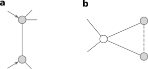
Figure 1: Diverse dynamic impact of structural links on effective connectivity. (a) Structural links may not be detectable by certain correlation measures due to strong independent driving signals (e.g. noise). For example, strong inputs along two links (from within or outside the network, marked by arrows) may decorrelate the dynamics of the two nodes (gray disks) although they directly interact. (b) Common input may create effective link without the structural link present. For example, common input from a third node (open circle) may create effective connectivity (dashed line) between two nodes (gray disks) that are not directly connected. In both examples, (a) and (b), it may depend on the entire collective state of the network (and the external inputs it may receive) whether or not an effective connection is detected.

Structural connectivity may be very different from effective or functional connectivity (Figure 1). On the one hand, high correlations may exist between two units that are not directly connected but only influenced by each other via a third unit they both directly interact with. In general, such indirect interactions may be induced not only by one third node, but equally by the entire collective dynamics of a network. On the other hand, even a strong direct interaction between two units does not necessarily mean that their dynamics is highly correlated; correlations could be submerged, e.g., by external noise or recurrent inputs the two units receive, e.g., from two distinct other parts of the network, or even from outside of it.

In general, effective and structural connectivity are related in a highly non-trivial way. In fact, a number of counter-intuitive phenomena have been observed in various systems. For instance, recent work on coupled oscillator networks highlight that under certain conditions noise may aid to reconstruct structural connectivity from correlation-based effective connectivity [15]; and one may detect small world features in the functional connectivity even if it is derived from randomly connected dynamical systems without any specific small-world features [16].

Where do we start from? It is important to clarify which knowledge about the networked system we presuppose. Is the collective dynamics known to be simple such as converging to a fixed point of concentrations in biochemical networks or to a limit cycle in coupled oscillator networks? Or do we expect more complex, irregular, and perhaps unpredictable, chaotic or random types of dynamics? Can we change the dynamics of units by interfering with the system or can we just observe? Does the research question require a global analysis in state space or do we focus on a specific dynamical state where local analysis may suffice? We should answer these questions, among others, before using or developing any inference method – to achieve reconstruction at the level we need with best quality and minimal efforts, both experimentally and computationally.

Here we review recently developed approaches to inferring structural connectivity of a network from accessing its collective dynamics. The presented approaches assume various levels of pre-knowledge about the system and may or may not require the observer to interfere with the system. The article is structured as follows. We first clarify in Section 2 what we mean by a network dynamical system, taking the view of continuous-time dynamics described by coupled ordinary differential equations. In Sections 3, 4, and 5, we explain three principally different classes of methods to obtain information about the structure of the network topology from dynamical quantities.

Section 3 illustrates basic theoretical approaches based on measuring and evaluating the response of a network to external perturbations or driving. As the response depends on both the external driving signal and the interaction topology of the network, sufficiently many driving-response experiments yield information about the entire network topology. A second class of methods sets up a model copy of the original system (Section 4) and adapts the coupling matrix of the model so as to synchronize its dynamics with the original. If synchronization is achieved, the topology obtained for the model is taken as a proxy for the original. Finally, a set of direct methods (Section 5) rely on measuring time series (or features thereof), evaluating temporal derivatives, and exploiting smoothness assumptions to find solutions to an optimization problem given by the restrictions by data.

We briefly comment on technical issues (Section 6) and mention basic core approaches for identifying effective connectivity (Section 7). These approaches rely on simple linear correlation, maximum entropy principles and related statistical inference methods. Finally, we provide an outlook (Section 8) where we highlight current challenges, point out aspects sometimes overlooked and show potential research paths towards uncovering more of the topology of the networks that surround us.

This review on purpose is short but self-contained. It is intended for researchers mainly in the physical and biological sciences and engineering and assumes basic knowledge of dynamical systems and probability theory. Let’s start with the details.

2 Nonlinear dynamics of networks

2.1 Systems of ordinary differential equations describing networks

Throughout the main part of this review, we consider networks of units assumed to be described by systems of ordinary differential equations. Discrete time maps coupled to a network are not discussed but typically approaches similar to those presented here are viable in slightly modified form. We discuss specific issues for systems of pulse-coupled units, such as spiking neurons, in section 5. These are formally hybrid systems, i.e. mixtures of continuous-time and discrete time systems.

Assuming that interactions occur between pairs of coupled units, a generic network dynamical systems is given by

$$\frac{d}{dt}\boldsymbol{x}_{i}=\boldsymbol{f}_{i}\left(\boldsymbol{x}_{i}\right)+\sum_{j=1}^{N}J_{ij}\boldsymbol{g}_{ij}\left(\boldsymbol{x}_{i},\boldsymbol{x}_{j}\right)+\boldsymbol{I}_{i}(t)+\boldsymbol{\xi}_{i}(t)$$ (1)

where $i,j\in\{1,2,\ldots N\},$ $\boldsymbol{x}_{i}(t)=\left[x_{i}^{(1)}(t),x_{i}^{(2)}(t),\cdots,x_{i}^{(D)}(t)\right]^{\mathsf{T}}\in\mathbb{R}^{D}$ describes the state of the $i$-th unit at time $t\in\mathbb{R}$, and the functions $\boldsymbol{f}_{i}:\,\mathbb{R}^{D}\rightarrow\mathbb{R}^{D}$ and $\boldsymbol{g}_{ij}:\,\mathbb{R}^{D}\times\mathbb{R}^{D}\rightarrow\mathbb{R}^{D}$ mediate intrinsic and interaction dynamics of the D-dimensional units, respectively. The term $\boldsymbol{I}_{i}(t)$ represents a vector of external driving signals (possibly random) and $\boldsymbol{\xi}_{i}(t)$ symbolically represents external noise. Finally, the $J_{ij}$ define the interaction topology, in the simplest setting in terms of the adjacency matrix $A$ such that $J_{ij}=A_{ij}=1$ if there is a direct physical interaction from unit $j$ to $i$ and $J_{ij}=A_{ij}=0$ otherwise. In general, units’ interaction may be higher order, e.g. requiring terms like $\boldsymbol{h}_{ijk}\left(\boldsymbol{x}_{i},\boldsymbol{x}_{j},\boldsymbol{x}_{k}\right)$ added to the right hand side of (1). For instance in gene and protein interaction networks, a protein (the so-called transcription factor, say unit $k$) is directly influencing the rate of transcription of a gene (say, unit $j$) to a DNA segment (say unit $i$). We do not treat such terms here explicitly. Their relevance for network dynamical systems is discussed in [17].

For some methods to infer effective connectivity, the functional form of (1) does not directly enter the inference argument, other methods can be extended to include higher order terms explicitly. We comment on higher order terms where appropriate (cf. also Sect. 5).

2.2 Rescaling, simplifications, and common interactions

Some a priori technical issues: Considering (1) as our basic level of description, in case the dimension $D_{i}$ of the local dynamical system $i$ depends on unit $i$, we would just consider the maximal occurring dimension $D=\max_{i\in\{1,\ldots,N\}}D_{i}$ and for each unit ignore the $D-D_{i}$ dummy variables. This is done purely for notational simplification. Note further that in general, the quantity $J_{ij}$ is a $D\times D$ matrix of coupling strengths $J_{ij}^{dd^{\prime}}$, but that for many paradigmatic model systems, only one of these elements is non-zero, i.e. $J_{ij}^{dd^{\prime}}=J_{ij}^{dd^{\prime}}\delta_{d,d_{1}}\delta_{d^{\prime},d_{2}}$such that $J_{ij}=J_{ij}^{d_{1}d_{2}}$ is sufficient to describe the influence of unit $j$ on $i$.

Given a dynamical system of the form (1), the right hand side is determined up to $N\times D$ additive constants $C_{i}^{d}$ and one overall multiplicative constant $C_{0}$. Shifting the state variables $x_{i}^{d}$ to co-moving frames and rescaling time enables us to set $C_{i}^{d}=0$ for all $i$ and all $d$ and $C_{0}=1$ without loss of generality.

For simplicity of presentation, we furthermore describe the methods below as if they were for networks of coupled one-dimensional units only. Often, different dimensions may be treated independently during reconstruction.

We thus take the coupled equations

$$\boxed{\frac{d}{dt}x_{i}=f_{i}\left(x_{i}\right)+\sum_{j=1}^{N}J_{ij}g_{ij}\left(x_{i},x_{j}\right)+I_{i}(t)+\xi_{i}(t)}$$ (2)

as our basic network characterization we start from, where now the variables $x_{i}$ and $x_{j}$ and the functions $f_{i}$ and $g_{ij}$ are treated as real scalars.

Common Interaction Functions. Only non-trivial coupling terms that are not identically zero,

$$\frac{\partial g_{ij}}{\partial x_{j}}\neq 0$$ (3)

for the relevant domain of arguments actually contribute to interactions, so we assume all coupling functions $g_{ij}$ for which $J_{ij}\neq 0$ to be non-trivial in this sense. A broad range of systems exhibits diffusive coupling such that

$$g_{ij}\left(x_{i},x_{j}\right)\propto\left.\left(x_{j}-x_{i}\right)\right.$$ (4)

which is a special case of coupling functions

$$g_{ij}\left(x_{i},x_{j}\right)=\left.\tilde{g}_{ij}\left(x_{j}-x_{i}\right)\right.$$ (5)

that depend on state differences (e.g. phase differences for coupled oscillators) only. The simplest non-trivial form of interaction is linear coupling,

$$g_{ij}\left(x_{i},x_{j}\right)=A_{ij}x_{j}\,,$$ (6)

and does not depend on the dynamical variable of the unit it influences.

We have now set the stage to dive into specific inference approaches.

3 Driving-response experiments

One idea of inferring network topology is to measure the collective response of a network dynamical system to driving by external signals. For instance, if a system exhibits a stable collective state (e.g. fixed point or periodic orbit, cf. Fig. 2), it will relax back to that state after a transient input (pulse), if the latter is not too strong (such as to not kick the system out of the basin of attraction of the stable state) [18, 19, 20, 21, 22]. Here, the input signal (driving) effectively changes the initial condition of the system, leaving the system features (given by the local and interaction functions and their parameters) the same. Similarly, a stable state of the system will generically move in state space (and keep qualitatively the same stability properties) in response to sufficiently weak, temporally constant external perturbations. These kinds of perturbations effectively creates a non-identical but similar systems with different parameters determined by the driving signal.

Both the relaxation dynamics and the shift in state space in general depend not only on the external signal (which unit is perturbed, how and how strongly, i.e. known quantities), but also on the (unknown) interaction topology of the network. Each collective response of the system to an external perturbation yields a restriction on the network topology such that sufficiently many driving-response experiments may reveal the entire topology. In this section, we present the main ideas underlying several related driving-response approaches.

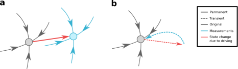
Figure 2: Stable state approaches to network inference. (a) Constant external driving signal (parameter change) moves the stable fixed point (gray) in state space to another position (blue). The difference vector $v$ (red) depends on both the driving signal and the network topology such that several measurements of $v$ under different driving conditions yields information about the topology. (b) Same as (a) but for transient perturbative signal: After the driving signal is switched off, the dynamics relaxes back (dashed blue trajectory) towards the original fixed point (gray). Now, the relaxation trajectory contains information about the topology.

3.1 Restrictions from local fixed point analysis

Recent efforts for developing methods to identify a network’s topology have emerged from the need to understand biological, in particular gene regulatory networks [1, 23, 24, 25]. Such networks consist of genes and proteins that interact with each other within a cell [26, 27]. These interactions in particular control (indirectly) the rates at which genes are transcribed into mRNA and the regulatory features emerge via the interactions and generally do not follow from the single-gene level [28]. Gene regulatory networks and other reaction networks, e.g., in chemistry or population dynamics, are often modeled by nonlinear differential equations

$$\dot{z}_{i}=f_{i}(z_{1},z_{2},\ldots,z_{N};\boldsymbol{p},\tilde{\boldsymbol{I}}),$$ (7)

describing the rate of change of the expected numbers (or concentrations) $z_{i}(t)$ of entities (e.g. genes, atoms and molecules or individual organisms) at time $t$ in terms of their dependence on the number of other entities [27]. Here $\boldsymbol{p}$ is a set of parameters and $\tilde{\boldsymbol{I}}$ represents a set of external perturbations directed to the entities. The $z_{i}$ are typically positive real numbers but mathematically there is no restriction for them to also be negative. Under the assumption that such a system is close to a steady state $\boldsymbol{z}^{*}=(z_{1}^{*},z_{2}^{*},\ldots,z_{N}^{*})$, a stable fixed point where $f_{i}(z_{1},z_{2},\ldots,z_{N};\boldsymbol{p},\tilde{\boldsymbol{I}})=0$ for all $i$, the dynamics for perturbations $x_{i}(t)=z_{i}(t)-z_{i}^{*}$ from steady state concentrations of such nonlinear models may be approximated to first order in the $x_{i}$ by

$$\dot{x}_{i}=\sum_{j=1}^{N}J_{ij}x_{j}+I_{i}(t),$$ (8)

where the local Jacobian $J_{ij}=(\partial f_{i}/\partial z_{j})(\boldsymbol{z}^{*})$ is the effective interaction matrix given the steady state and $I_{i}(t)$ is assumed to be an external perturbation linearly coupling to deviations of variables $x_{i}$. We remark that when deriving (8) from (7) we implicitly use the relation

$$I_{i}(t)=\sum_{j}\tilde{I}_{j}(t)\left.\frac{\partial f_{i}}{\partial\tilde{I}_{j}}\right|_{\boldsymbol{z}=\boldsymbol{z}^{*},\tilde{\boldsymbol{I}}=\mathbf{0}}+\mathcal{O}\left(\tilde{I}_{i}\tilde{I}_{j}\right)$$ (9)

ignoring the second and higher order terms.

3.1.1 Driving the system constantly to move a stable state
(changing parameters)

The method presented now effectively moves the parameters and thus in particular the fixed points of a system. Originally intended for gene and protein interaction networks, Gardner and coworkers [1, 29] have explicated that reconstruction is possible, at least for small networks. We here discuss two approaches of using the general form (8) to reconstruct the interaction network, i.e. the $J_{ij}$. The first is based on driving the system (8) by sufficiently small, temporally constant driving forces $I_{i}(t)=I_{i,m}$ to new fixed points $x_{i,m}^{*}\neq 0$ close to the original one $x_{i}^{*}=0$. As the original fixed point was structurally stable, the new fixed point will generically exist and have qualitatively the same stability properties if the $I_{i,m}$ are small enough (Fig. 2a). This is because solutions of (7), in particular fixed point solutions, typically vary continuously with changing parameters (here: changing $I_{i,m}$ from zero) and there is no bifurcation close to the parameters yielding a generic stable fixed point $y_{i}^{*}$.

The observed values assumed at each new steady state together with the (known) driving signals provide information about the interaction topology $J_{ij}$. Performing several perturbation experiments $m\in\{1,\ldots,M\}$ yield $N\times M$ equations

$$\sum_{j=1}^{N}J_{ij}x_{j,m}^{*}=-I_{i,m},$$ (10)

one for each experiment $m$ and for each unit $i$.

After an arbitrary number $M$ of experiments, eq. (10) in matrix form becomes

$$JX=Y,$$ (11)

where $J\in\mathbb{R}^{N\times N}$ represents the connectivity among the units, $X\in\mathbb{R}^{N\times M}$ the steady state values with $X_{i,m}=x_{i,m}^{*}$, and $Y\in\mathbb{R}^{N\times M}$ the perturbations $Y_{i,m}=-I_{i,m}$ that we assume to be known. This matrix equation restricts the connectivity $J$ given the measured data $X$ and the input perturbations $I$. The matrix equations constraining the full network topology $J$ can be split into $N$ equations

$$\boldsymbol{J}_{i}X=\boldsymbol{Y}{}_{i}\,,$$ (12)

one for each input connectivity $\boldsymbol{J}_{i}:=(J_{i,1},\ldots,J_{i,N})\in\mathbb{R}^{1\times N}$ of a unit $i$. Thus, the same set of data $X$ restrict all the sets of units providing interactions to $i\in\{1,\ldots,N\}$ but the data $\boldsymbol{Y}{}_{i}=(Y_{i,1},\ldots,Y_{i,M})^{\textsf{T}}$ are unit dependent. This reduction to $N$ individual equations also admits to split the computational effort for solving them. The problem becomes trivially parallelizable because for different $i$, these restrictions (12) are independent in the sense that reconstruction of the input coupling strengths to each unit $i$ can be performed without taking care of input coupling strengths of other units $k\neq i$.

3.1.2 Observe relaxation to stable state after transient driving
(changing initial conditions)

A second approach assumes that the quantities $y_{i}$ (and thus the $x_{i}$) are perturbed such that at time $t_{0}$ we have $x_{i}(t_{0})=x_{i}^{(0)}$ and the transient dynamics $y_{i}(t)$ of relaxation back to the original fixed point $y_{i}^{*}$ (and thus $x_{i}^{*}=0$) are observed at a sequence of times $t_{m}>t_{0}$, $m\in\{1,\ldots,M\}$. This yields the same type of equation (11), but now with the $Y_{i,m}=-\hat{\dot{x}}_{i,m}$ being estimated of the derivatives $\dot{x}{}_{i}(t_{m})$. We remark that these derivatives may be estimates in various ways, each of them requiring a resolution of the measured data on sufficiently small time scales, cf. section 5.1. In this second approach, the different times the transient dynamics is measured replaces the different driving experiments in the first approach. Finally, both approaches can of course be combined, several experiments evaluated at several time points, again yielding the same form of restrictions (11).

3.2 Solving the restricting equations

How can we finally obtain the coupling elements $J_{ij}$ and thus the interaction network? In principle, solving the matrix equation (11) yields the interaction matrix $J$ as a function of the known data $X$ and $Y$. One may naively assume that it is directly solvable once the number of experiments equals the number of units in the network, $M=N$. However, this problem can be numerically ill-conditioned [30] for large $N$, such that the result is not reliable. In addition, as also stressed in [1], the results may be sensitive to noise in the measured data.

A way to overcome this problem is by performing (many) more experiments than nodes available, $M\gg N$, thus over-determining (11). In general, due to noise and measurement inaccuracies, this yields the system (12) to be inconsistent such that there is no vector $\boldsymbol{J}_{i}$ that satisfies all constraints. It will still be possible to find a robust approximation $\boldsymbol{\hat{J}}_{i}$ that minimizes the error between the predicted dynamics $\boldsymbol{J}_{i}X$ and the actual dynamics $\boldsymbol{Y}{}_{i}$ for a given node. Specifically, this error function may be modeled as

$$E_{i}(\boldsymbol{\hat{J}}_{i})=d(\boldsymbol{Y}_{i},\,\boldsymbol{\hat{J}}{}_{i}X),$$ (13)

where the distance measure $d(\boldsymbol{v},\boldsymbol{w})=\|\boldsymbol{v}-\boldsymbol{w}\|_{p}^{p}$ between two vectors $\boldsymbol{v},\boldsymbol{w}\in\mathbb{R}^{M}$ is commonly defined in terms of the $p$th power

$$d(\boldsymbol{v},\boldsymbol{0})=\|\boldsymbol{v}\|_{p}^{p}=\left(\sum_{m=1}^{M}v_{m}^{p}\right)$$ (14)

of an $L_{p}$-norm with $p\geq 1$, due to its convexity properties. This guarantees that any local minimum of $E_{i}$ is also a global minimum [31]. Particularly, the $L_{2}$-minimization criterion,

$$E_{i}(\boldsymbol{\hat{J}}_{i})=\|\boldsymbol{Y}_{i}-\boldsymbol{\hat{J}}{}_{i}X\|_{2}^{2},$$ (15)

is of great importance because it has an analytical solution for its extremum. Equating to zero the derivatives of the error function with respect to the matrix elements, $\frac{\partial}{\partial J_{ik}}E_{i}\left(\boldsymbol{\hat{J}}{}_{i}\right)\stackrel{{\scriptstyle!}}{{=}}0$, yields an analytical solution (see Appendix A) to $L_{2}$ error-minimization given by

$$\boldsymbol{\hat{J}}{}_{i}=\boldsymbol{Y}{}_{i}X^{\mathsf{T}}(XX^{\mathsf{T}})^{-1}.$$ (16)

Evaluating such equations for all $i\in\{1,\ldots,N\}$ yields the complete reconstructed network $\hat{J}$. This mathematical form of minimum $L_{2}$-norm solution is implemented in many mathematical packages (e.g. as the mrdivide function in Matlab [32] or the LeastSquares function in Mathematica [33]). We explicate that the obtained off-diagonal terms $\hat{J}_{ij}$ serve as the best estimate (in the procedural sense using the $L_{2}$-minimization above) for the coupling constants $J_{ij}$ ; at the same time, the diagonal elements $J_{ii}$ are not relevant for the network topology because the influence of these terms on the dynamics of unit $i$ is physically indistinguishable from an intrinsic drive to $i$ included in the local dynamics specified by $f(x_{i})$ in (2), cf. eq. (3).

Experimentally, it is in principle possible to over-determine a system of equations by performing repeated measurements on the network until the condition $M\gg N$ is achieved. Nevertheless, it may often seem unsuitable for large networks due to the large number of experiments that would be required.

So, if the size of the network is an issue or the number of available measurements insufficient to over-determine the system, we have $M<N$. Assuming that the network is sparse (i.e. that each unit is connected with a small number of others and thus many connection strengths are $J_{ij}=0$), may still yield the collection of all network links. This implies that several $J_{ij}$ are effectively set to zero, therefore decreasing the amount of unknown coefficients to be solved for. It leaves us with the problem of finding which links are actually present and which are not. We present two related options to do so.

3.2.1 Sparse solution with a bounded connectivity per unit

If an upper bound for the number of links $K_{i}<M$ is known, we may assume only $M<N$ experiments are available and we have a rough idea of how many nodes (at most) are connected to a particular node. In particular, assume that the number of incoming connections for node $i$ is given by at most $K_{i}<M$ [1]. This assumption shifts the system (12) from having more unknowns than constraints, $M<N$, to have more constraints than unknowns, $M>K_{i}$, therefore, implicitly over-determining the system. It means that out of the $N$ nodes present in the network only $K_{i}$ of them are chosen to be part of the system of equations for node $i$. Such assumption may be done when there is some a priori information about the network’s connectivity and dynamics.

Specifically, the system of equations (12) may in principle be rewritten as

$$\boldsymbol{B}_{i}Z_{i}=\boldsymbol{Y}{}_{i},$$ (17)

where $\boldsymbol{B}_{i}\in\mathbb{R}^{1\times K_{i}}$ is the reduced connectivity vector for node $i$ that contains the coupling strengths for the selected nodes and $\boldsymbol{Z}_{i}\in\mathbb{R}^{K_{i}\times M}$ is a matrix that contains the states of such nodes. If we knew which $K_{i}$ of the $N-1$ possible connections actually contributed, we could use eq. (16) to solve (17) using $L_{2}$-minimization yielding

$$\hat{\boldsymbol{B}}_{i}=\boldsymbol{Y}{}_{i}Z_{i}^{T}(Z_{i}Z_{i}{}^{T})^{-1},$$ (18)

where $\hat{\boldsymbol{B}}_{i}$ is the best approximation to $\boldsymbol{B}_{i}$.

Yet, it so far remains unclear which of the $\binom{N}{K_{i}}=\frac{N!}{K_{i}!(N-K_{i})!}$ possible combinations of incoming connections is best suited for reproducing the dynamics of $i$. In principle, $\hat{\boldsymbol{B}}_{i}$ may be calculated for each combination of $K_{i}$ genes, and the combination that yields the smallest value of the $L_{2}$ norm $\left\|\hat{\boldsymbol{B}}_{i}\right\|_{2}$ in (18) may be chosen as the best estimate for $J_{i}$. The efficiency of such a procedure relies in number $K_{i}$ of interactions per node. Hence, choosing a proper $K_{i}$ aiming to recover the largest number of real interactions with the smallest number of false positives is a key factor to achieve a successful topological reconstruction.

3.2.2 Maximizing the sparseness of the connectivity matrix

If $M<N$ and the $K_{i}$ are unknown, cannot be estimated or there are too many of them (making the combinatorial search practically impossible) maximizing the number of zero entries in $\boldsymbol{J}$, (i.e. minimizing the $K_{i}$ and thus maximizing sparseness) may be a way to solve (12). This approach is particularly useful if the only a priori knowledge about the network’s connectivity is some sparsity.

For general matrix equations

$$A\boldsymbol{y}=\boldsymbol{b},$$ (19)

where $A\in\mathbb{R}^{m\times n}$, $\boldsymbol{y}\in\mathbb{R}^{n\times 1}$ and $\boldsymbol{b}\in\mathbb{R}^{m\times 1}$, singular value decomposition (SVD) of $A$ according to

$$A=U\Sigma V{}^{\mathsf{T}},$$ (20)

yields an analytic solution

$$\boldsymbol{y}=V\tilde{\Sigma}U{}^{\mathsf{T}}\boldsymbol{b}+V\boldsymbol{c},$$ (21)

where $\tilde{\Sigma}=\Sigma^{\mathsf{T}}\left(\Sigma\Sigma^{\mathsf{T}}\right)^{-1}$that parametrizes the space of all solutions through the vector $\boldsymbol{c}\in\mathbb{R}^{n\times 1}$ with $c_{i}=0$ for $i\in\{1,...,r\}$ and $r=Rank(\boldsymbol{A})$.

In our reconstruction problem, we are seeking to maximize the number of zero entries in $\boldsymbol{J}$ based on solving the restricting equations (12) for $\boldsymbol{J}{}_{i}$ as we solved (19) for $\boldsymbol{y}$. Consider the transpose

$$X^{\mathsf{T}}\boldsymbol{J}_{i}^{\mathsf{T}}=Y{}_{i}^{\mathsf{T}}$$ (22)

of (12). The analogous SVD-based solution then reads

$$\boldsymbol{J}{}_{i}^{\mathsf{T}}=V\tilde{\Sigma}U{}^{\mathsf{T}}\boldsymbol{Y}{}_{i}^{\mathsf{T}}+V\boldsymbol{c},$$ (23)

where $U\in\mathbb{R}^{M\times M}$, $V\in\mathbb{R}^{N\times N}$, $\tilde{\Sigma}\in\mathbb{R}^{N\times M}$ and $\boldsymbol{c}\in\mathbb{R}^{N\times 1}$ is a vector of remaining coefficients parametrizing the solution space. Thus, the set of all possible solutions for $\boldsymbol{J}{}_{i}$ is given by (23). The goal now is to pick the sparsest solution from this set. Therefore, eq. (23) may be posed as the overdetermined ($M>N-r$) problem

$$V\tilde{\Sigma}U^{T}\boldsymbol{Y}_{i}^{T}=-V\boldsymbol{c}.$$ (24)

Minimizing the $L_{1}$ error

$$E_{i}(\boldsymbol{c})=\|V\tilde{\Sigma}U^{T}\boldsymbol{Y}_{i}^{T}+V\boldsymbol{c}\|_{1},$$ (25)

yields a sparse solution [31]. However, unlike the $L_{2}$ minimization, $L_{1}$ minimization has no analytical solution, so choosing an appropriate iterative algorithm to solve it is essential. The Barrodale Roberts algorithm [34] provides a particularly fast solver that has been vastly used in the field of network reconstruction [10, 12, 29, 35].

Remarks. The core equations (50) also provide the option to reconstruct network connectivity via maximizing sparseness of the network and there is a particular relation to what is known as compressive sensing cf., e.g. [36] .

In general, linearization of dynamical equations, e.g. linearizing in state variables close to fixed points, often well approximates nonlinear dynamics. This seems to hold for gene regulatory networks [29] as well as in models of Drosophila segmentation networks [37] and may thus be of general use across systems. For gene and protein interaction networks, often single genes are selected for perturbations in an experiment, with the danger of providing non-generic restrictions in (12). Finally, for some systems increasing the number of experiments may reduce the resulting computational costs such that this trade-in may be considered.

3.3 Driving the system’s state to a fixed point

One may also infer network structure by externally driving the system to a fixed point and shifting component values of the fixed point for individual units [38, 39]. As before, the differences between pairs of steady-state responses are analyzed. Let us describe the network as

$$\dot{x}_{i}=f_{i}(x_{i})+\sum_{j=1}^{N}A_{ij}g_{ij}(x_{i},x_{j})+I_{i},$$ (26)

where the $A_{ij}\in\{0,1\}$ are the entries of the adjacency matrix specifying only if an interaction from $j$ to $i$ is present ($A_{ij}=1$) or not ($A_{ij}=0$), the $g_{ij}(x_{i},x_{j})$ are the coupling functions from $j\in\left\{1,2,\ldots,N\right\}$ to $i$, and $I_{i}$ is the driving signal applied to unit $i$. It was demonstrated by Yu and Parlitz [38] that under driving signals

$$I_{i}=-\left(x_{i}-\hat{x}_{i}\right)\theta,$$ (27)

with sufficiently large gain factor $\theta\in\mathbb{R}$ and Lipschitz continuous $f_{i}$ and $g_{ij}$ , the network may be driven to a globally stable fixed point $\boldsymbol{x}^{*}:=(x_{1}^{*},x_{2}^{*},\ldots,x_{N}^{*})^{\mathsf{T}}\in\mathbb{R^{N}}$ that is arbitrarily close to a predetermined point $\hat{\boldsymbol{x}}:=(\hat{x}_{1},\hat{x}_{2},\ldots,\hat{x}_{N})^{\mathsf{T}}\in\mathbb{R^{N}}$, independent of the initial conditions [38] . At such fixed point we have

$$(x_{i}^{*}-\hat{x}_{i})\theta=f_{i}\left(x_{i}^{*}\right)+\sum_{j=1}^{N}A_{ij}g_{ij}\left(x_{i}^{*},x_{j}^{*}\right)$$ (28)

for all $i$. To understand how the network responds to changes in $\hat{\boldsymbol{x}}$, let us define

$$\Delta_{i}:=f_{i}(\hat{x}_{i})+\sum_{j=1}^{N}J_{ij}g_{ij}\left(\hat{x}_{i},\hat{x}_{j}\right)-\left[f\left(x_{i}^{*}\right)+\sum_{j=1}^{N}J_{ij}g_{ij}\left(x_{i}^{*},x_{j}^{*}\right)\right],$$ (29)

hence, eq. (28) may be rewritten in terms of $\Delta_{i}$ as

$$\left(x_{i}^{*}-\hat{x}_{i}\right)\theta=f_{i}(\hat{x}_{i})+\sum_{j=1}^{N}A_{ij}g_{ij}\left(\hat{x}_{i},\hat{x}_{j}\right)-\Delta_{i}.$$ (30)

The main idea at this point is to check whether unit $k$ couples to unit $i$ by evaluating how $x_{i}^{*}$ reacts to the shifting of $x_{k}^{*}$ through $\hat{x}_{k}$. Therefore, let us set

$$\hat{x}_{j}=\begin{cases}\hat{x}_{k}&\mbox{if }j=k\\ 0&\mbox{if }j\neq k\end{cases},$$ (31)

and evaluate (30) at this point, yielding

$$x_{i}^{*}\theta=A_{ik}g_{ik}\left(0,\hat{x}_{k}\right)-\Delta_{ik}+f_{i}(0)+\sum_{j\neq k}^{N}A_{ij}g_{ij}\left(0,0\right).$$ (32)

Shifting the same component twice to $\hat{x}_{k}^{(1)}$ and $\hat{x}_{k}^{(2)}$, resp., fixes a reference frame and thereby yields equations characterizing the difference between responses of a given unit $i$ to a shifted fixed point component for unit $k$. It results in

$$\left[x_{i,2}^{*}-x_{i,1}^{*}\right]\theta=A_{ik}\left[g_{ik}\left(0,\hat{x}_{k,2}\right)-g_{ik}\left(0,\hat{x}_{k,1}\right)\right]+[\Delta_{ik,1}-\Delta_{ik,2}],$$ (33)

a condition that may be rewritten as

$$S_{ik}\theta=A_{ik}\eta_{ik}+\lambda_{ik}.$$ (34)

We remark that the differences $[\Delta_{ik,1}-\Delta_{ik,2}]$ in (33) are not known but the general form (34) may be used to reveal whether they are zero, $\lambda_{ik}=0$, or not: Given that we are dealing with entries of the adjacency matrix, we may infer two possible outcomes from (34), whether system $k$ is coupled to $i$ or not. Specifically,

$$S_{ik}\theta=\begin{cases}\eta_{ik}+\lambda_{ik}&\text{if unit \mbox{\emph{k} coupled to \emph{i} }}\\ \lambda_{ik}&\text{if not}\end{cases}$$ (35)

It was also demonstrated by Yu and Parlitz [38] that $\Delta_{i}$ decreases with $\theta$ if $f_{i}$ and $g_{ij}$ are Lipschitz continuous. This permits to discriminate whether there is a coupling between a pair $k\rightarrow i$. Especially, when $\theta$ is sufficiently large, the $|S_{ik}\theta|$ values may be classified into sets $\mathbb{I}_{0}$ and $\mathbb{I}_{1}$, non-coupled and coupled sets, respectively. To construct such sets, Yu and Parlitz [38] propose to:

• For fixed $k,$ organize the $|S_{ik}\theta|$ values in an ascending order, i. e., the values should be arranged into a new series $z$ where $z_{k,j}<z_{k,j+1}<\ldots$ that defines the indexing $j$ of the $z_{k,j}$’s.

• Establish the critical values of each set. In this case, the critical values $j_{c}$ and $j_{c+1}$ define the end and the beginning of $\mathbb{I}_{0}$ and $\mathbb{I}_{1}$, respectively. Yu and Parlitz suggest to find $j_{c}$ by requiring the distance between any element from $\mathbb{I}_{1}$ with respect to $z_{i,1}$ to be larger than twice the size of $\mathbb{I}_{0}$, $z_{k,j}-z_{k,1}\geq 2(z_{k,j_{c}}-z_{k,1})$ for all $j>j_{c}$.

Finally, by performing this process on every unit, the topology of the network may be reconstructed.

Remarks: The approach relies on the feasibility of (i) perturbing the systems in a specific manner, and (ii) measuring the steady states, suggesting that it is model independent to a large extent in that it does not in principle require knowledge of local dynamics or coupling functions (yet it requires these to be Lipschitz continuous). These features may make the approach of interest under certain conditions where only little pre-knowledge about the system is available. Yet the approach requires substantial control over the system, in particular, the option of externally driving every unit (independently) constitutes a major requirement. The study [38] does not state how indirect actions are treated, for instance, how is an indirect effect from unit $k$ via $k^{\prime}$ onto $i$ distinguished from direct interactions from $k$ to $i$? Possibly, driving $k$ may indirectly affect $i$ only weakly and this potentially second order contribution could be treated in a perturbative way.

3.4 Distributed perturbations to collective periodic dynamics

The approaches presented above (sections 3.1-3.3) required the existence of fixed points either in the original system or in the presence of sufficiently strong external driving. Yet, more complex dynamics prevails in a large range of biological, physical or artificial systems. The second most simple invariant dynamics are periodic orbits and often arise as limit cycles of coupled oscillatory units, thus asking for a generalization beyond simple fixed point approaches. Even more complex dynamics, e.g. collective chaos, is treated by a direct approach below in section 5.1.

Is it possible to infer network topology from driving-response experiments also for oscillator networks? Below we positively answer this question, at the same time showing that distributed driving signals not precisely targeted to one or a few units are at least equally appropriate to infer network topology. Several theoretical model studies of coupled oscillators [40, 41, 42, 43, 44, 45] have shown that the response of single units in a network to constant or periodic driving signals as well as the transient dynamics of synchronization depend on the network topology. Some recent works [43, 44] helped us to understand specific quantitative influence of structural features on the response and how the network response provides some information about the structure (and the driving signal). For instance, the magnitude of responses seem to decay exponentially with distance from the driving node [43], and the coarse-scale connectivity among connected components may qualitatively determine to which degree network dynamics is coordinated globally [44]. Further developing such insights, a follow-up work [10] presents a method of reconstructing network topology from systematic measurements of network responses to temporally constant, distributed driving signals in coupled phase-oscillator networks.

The basic idea is that any network displaying a stable invariant dynamics, not just fixed points, yield a specific response to a given perturbation as a consequence of the network’s topology and the perturbation itself [40, 42, 44] cf. Fig. 3. If the perturbations are small, the invariant set is typically qualitatively unchanged and only slightly moved in state space. Keeping track of which driving signals resulted in which responses, we can collect evidence about the interactions among units in a network. Sufficiently many repetitions of appropriate driving-response experiments then yield the network’s topology.

Weakly coupled limit cycle oscillators are well-characterized by ignoring (in the long time limit) amplitude responses to coupling and by modeling them as phase-oscillators with coupling via their phase-differences only. A method to infer network topology for coupled phase oscillators with arbitrary stable, phase-locked dynamics has been presented in [10]. One key observation is that the phase differences (yet not the phases themselves) in such systems converge with time and that comparing differences of phase differences among different driving conditions yield restrictions to network topology. The network dynamics is given by

$$\dot{\phi}_{i}=\omega_{i}+\sum_{j=1}^{N}J_{ij}g_{ij}(\phi_{j}-\phi_{i})+I_{i,m},$$ (36)

where $\phi_{i}(t)$ and $\omega_{i}$ are the phase and natural frequency of oscillator $i$, respectively, $J_{ij}$ the connection strength from oscillator $j$ to $i$ and $I_{i,m}$ is a temporally constant driving signal applied to $i$ during the experiment $m$. We assume that in the absence of driving, $I_{i,m}\equiv 0$, the network is in a phase-locked state where $\dot{\phi}_{j}-\dot{\phi}_{i}=0$ for all $i,j$. We remark that one, several or all units may be perturbed during each given experiment, such that driving can be arbitrarily distributed and effectively changes the frequencies of the driven oscillators. As for the approaches relying on fixed points (section 3.1), the existence of a stable periodic orbit (and thus in particular a phase-locked state) implies that sufficiently small constant perturbations yield a (only slightly moved and slightly different) stable periodic orbit.

If for a given driving condition $m$, the dynamics becomes phase-locked, the phase differences

$$\Delta_{ij,m}(t)=\phi_{j,m}(t)-\phi_{i,m}(t)$$ (37)

become constant in time, $\Delta_{ij,m}(t)\rightarrow\Delta_{ij,m}^{*}:=\lim_{t\rightarrow\infty}\left(\phi_{j,m}(t)-\phi_{i,m}(t)\right)$ because all oscillators move at the same collective frequency

$$\Omega_{m}=\omega_{i}+\sum_{j=1}^{N}J_{ij}g_{ij}(\phi_{j,m}-\phi_{i,m})+I_{i,m}.$$ (38)

Figure 3: Topology revealed by driving a stable periodic orbit: As for fixed point approaches discussed above (Section 3.1 and Fig. 2), the difference vector $v$ (red) depends on both the driving signal and the network topology such that several measurements of $v$ under different driving conditions yields information about the topology.

Hence, if the network is perturbed by a sufficiently small driving signal, the original phase-locked state (for $I_{i,m}\equiv 0$) is slightly moved such that $|\Delta_{ij,m}^{*}-\Delta_{ij,0}^{*}|\ll 1$ and there is a small difference between the perturbed and non-perturbed collective frequencies $\Omega_{m}$ and $\Omega_{0}$. Defining the effective frequency difference $D_{i,m}:=\Omega_{m}-\Omega_{0}-I_{i,m}$ of oscillator $i$, and approximating the arbitrarily nonlinear coupling functions $g_{ij}$ by a first order Taylor expansion around $\Delta_{ij,0}^{*}$ we obtain

$$D_{i,m}=\sum_{j=1}^{N}\hat{J}_{ij}\theta_{j,m}$$ (39)

where $\theta_{j,m}:=\phi_{j,m}-\phi_{j,0}$ is the phase shift and $\hat{J}$ is the Laplacian matrix of the network given by

$$\hat{J}_{ij}=\begin{cases}-J_{ij}g_{ij}^{\prime}(\Delta_{ij,0}^{*})&\mbox{for }i\neq j\\ {\displaystyle\sum_{k,k\neq i}}J_{ij}g_{ik}^{\prime}(\Delta_{ik,0}^{*})&\mbox{for }i=j.\end{cases}$$ (40)

Now, identifying the matrices $X_{i,m}=D_{i,m}$ and $Y_{i,m}=\theta_{i,m}$ we have reduced the problem of identifying network topology using distributed perturbations in systems of limit cycle oscillators to solving the same linear algebraic equation (11).

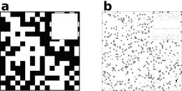
Figure 4: Revealing network topologies from response dynamics for directed networks of phase-locked Kuramoto oscillators. Variables evolve according to $\dot{x}_{i}=\omega_{i}+k^{-1}\sum_{j=1}^{N}J_{ij}\sin(x_{j}-x_{i})$, with random frequencies $\omega_{i}\in[0.1,1]$ and $k=8$ directed interactions of strengths $J_{ij}=k^{-1}$, randomly selected for each unit. Panels show reconstructed coupling matrices $J$ for (a) $N=16,$ and $M=32$, and (b) $N=64,$ and $M=32$. The matrices are gray-coded from white ($\hat{J_{ij}}$=0) to black ($\hat{J}_{ij}=\max_{i^{\prime}j^{\prime}}\{\hat{J}_{i^{\prime}j^{\prime}}\}$). Insets: Element-wise absolute difference $|J_{ij}^{\text{derived}}-J_{ij}^{\text{original}}|$, plotted on the same scale.

As remarked in previous sections, several experiments are necessary in order to perform the reconstruction of $\hat{J}$. Therefore, from repeated measurements for different conditions it is possible to rewrite eq. (39) in the form (11) in terms of $Y=D\in\mathbb{R}^{N\times M}$ and $X=\Theta\in\mathbb{R}^{N\times M}$ representing the differences between collective dynamics and phase shifts for each of the $N$ systems during the $M$ experiments.

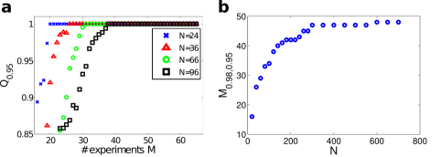
Figure 5: Quality of reconstruction and number of required experiments for reconstructing directed networks. Phase-locked Kuramoto oscillators with dynamics defined as in Fig. 4 with $k_{i}=10$ random incoming connections per node. (a) Quality of reconstruction at $\alpha=0.95$ for $N=24$ ($\times$), $N=36$ ($\vartriangle$), $N=66$ ($\circ$) and $N=96$ ($\square$). (b) Minimum number of experiments required for a reconstruction of quality level $q=0.98$ and accuracy $\alpha=0.95$.

Now, for sufficiently many experiments, i.e. $M\geq N$, the reconstruction may be accomplished in principle but may be ill-conditioned numerically. In addition, for large $N$ the many required experiments may not be practical. if this condition is not fulfilled, methods like the setting a maximum connectivity per system or maximizing the sparseness of the connectivity matrix (section 3.2.2), may be applied in order to make the problem of retrieving $\hat{J}$ an overdetermined problem.

As shown in [10], we may compare how accurate our prediction is by defining $J_{\max}:=\max_{i^{\prime}j^{\prime}}\left\{\left|J_{i^{\prime}j^{\prime}}^{\text{derived}}\right|,\left|J_{i^{\prime}j^{\prime}}^{\text{original}}\right|\right\}$, and using a relative difference defined as

$$\Delta J_{ij}:=\dfrac{1}{2J_{\max}}\left|J_{ij}^{\text{derived}}-J_{ij}^{\text{original}}\right|,$$ (41)

where $\Delta J_{ij}\in\left[0,1\right]\,\forall\,i,j$ . In addition, the quality of reconstruction $Q_{\alpha}$ may be posed as the fraction

$$Q_{\alpha}:=\dfrac{1}{N^{2}}\sum_{i,j}H\left((1-\alpha)-\Delta J_{ij}\right)\in\left[0,1\right]$$ (42)

of connection strengths which are assumed to be correct. Here $\alpha\leq 1$ is a constant employed to set the required accuracy for predictions and $H$ is the Heaviside function, $H(x)=1$ for $x\geq 0$ and $H(x)=0$ for $x<0$. For instance, $\alpha=0.95$ means that the derived matrix has a normalized relative error (41) of at most 5%. Moreover, we may estimate the minimum number of experiments

$$M_{q,\alpha}:=\min\left\{M|Q_{\alpha}(M)\geq q\right\}$$ (43)

required for a reconstruction with a quality level $q$ and with a prediction accuracy $\alpha$. Figure 5 illustrates these measures for random networks of phase-locked Kuramoto oscillators for several random topologies and parameters.

The driving response method in principle may be applied to a broad variety of problems involving stable dynamics. A model analogous to eq. (39) could be inferred as long as the systems may be linearized around a stable state, allowing to retrieve the topology from the network responses as above. Yet, there may be practical problems. For instance, even for perturbations induced by constant driving signals, the invariant solution resulting from perturbations to more complex periodic orbits or other stable invariant sets may be describable only by time dependent quantities (and not, e.g. temporally constant phase differences), limiting the approach suggested above to specific classes of systems.

3.5 Features and restrictions

One common advantage of the approaches presented above is that their required computational effort scales well (weaker than linearly) with system size $N$ such that at least moderately large systems appear accessible (cf. Figure 5). At the same time, the approaches are relatively simple to realize because they do not require knowledge in higher mathematics or computational approaches beyond a basic standard.

A possible route of generalization is to combine some of the above approaches. For instance, one may first drive a system to a stable fixed point as in section 3.1 and then apply small perturbations around that new point as in section 3.3.

Yet, all these approaches require the researchers to be able to access (measure and drive) the dynamics of all units in the system. Moreover, the local dynamics as well as the (approximate) form of interactions typically need to be at least partially known. The collective dynamics suitable for the driving-response approaches described above also need to be simple, in fact to exhibit a stable fixed point or periodic orbit or to admit the system to be driven to such as state. Finally, the presented inference of the existence of physical interactions and their functional form [46] seems well understood for networks of phase-oscillators, where perturbations in oscillation amplitude decays on faster time scale than the relaxation of phases. It thus remains an open problem how to use a driving response approach to properly infer structural network connectivity of coupled oscillators in systems, where the amplitude degrees of freedom play a role or are even dominant. More generally, systems exhibiting more complex dynamics, such asynchronous chaotic activity, bifurcations, multistability or other prevalent features of high-dimensional, nonlinear systems, currently still prevent network reconstruction by the methods presented above.

These requirements severely restrict the range of applicability in praxis to simple, well-accessible systems only. In particular for biological systems such as neural circuits or gene interaction networks, dynamics are typically more complex, systems are large and it is still hard to implement controlled large-scale driving experiments on the single-unit level. Direct methods (section 5) that do not rely on driving the system seem to offer viable directions towards reconstructing networks with such more complex dynamics as well. A currently open question of research constitutes how to exploit recorded time series from only a fraction of the units.

4 Copy-Synchronization: Adapting a model copy

Another way of reconstructing network topology of a given network is by adapting the topology of a second, model system, a network copy, such that it synchronizes with the original system. The idea is to update the model topology continuously until the copy system exhibits a dynamics identical to the original system; the rationale is that the final topology of the copy is likely to be the original topology [47].

Specifically, consider an (original) system of the form

$$\dot{x}_{i}=f_{i}(x_{i})+\sum_{j=1}^{N}J_{ij}g_{j}(x_{j}),$$ (44)

where $f_{i}$ and $g_{ij}$ are known and assumed to be Lipschitz continuous. This original system can in principle have arbitrary dynamics. Now, let us propose a model copy

$$\dot{y}_{i}=f_{i}(y_{i})+\sum_{j=1}^{N}K_{ij}g_{j}(y_{j})+I_{i},$$ (45)

where $y_{i}$ represents the state of the copy system, $I_{i}(t)$ are control feedback signals and $K_{ij}(t)$ is current coupling strength in the test system. In order to synchronize the copy to the original system, both the feedback signals $I_{i}(t)$ and the coupling strengths $K_{ij}(t)$ evolve in time and depend on the states of the actual and the copy system. Defining the synchronization error

$$e_{i}=y_{i}-x_{i}$$ (46)

we adapt the coupling strengths in the model copy according to

$$\dot{K}_{ij}=-\gamma_{ij}g_{j}(y_{j})e_{i}$$ (47)

and

$$I_{i}=-\alpha e_{i}$$ (48)

where $\alpha>0$ and $\gamma_{ij}>0$. We remark that here the local dynamics $f_{i}(.)$ as well as the coupling function $g_{ij}(.)$ need to be known in order to set up the test copy. It was proven in [47] that under feedback signals (48) with sufficiently large $\alpha$, the synchronization error $e_{i}$ decreases in time, $\dot{e}_{i}\leq 0$ for all $i$ such that the two systems converge to a synchronized state. The rationale is that after synchronization, the copy topology equals that of the original network, $K_{ij}\approx J_{ij}$, cf. Fig. 6. With minor modifications on the control signals $I_{i}$ this method admits to reconstruct networks and sub-networks in the presence of disturbances and modeling errors as well [47].

We remark that to the best of our knowledge, there is no guarantee that the resulting topology of the copy system actually reflects the one of the original network. In particular, symmetries might lead to disambiguities.

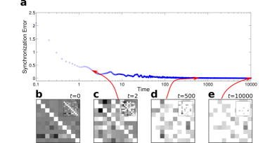
Figure 6: Revealing network topology via Copy Synchronization. Dynamics of reconstructed network for directionally coupled Kuramoto oscillators $\dot{x}_{i}=\omega_{i}+k^{-1}\sum_{j=1}^{N}J_{ij}\sin(x_{j}-x_{i})$ with random frequencies $\omega_{i}\in[-1,1]$, random coupling strengths $J_{ij}\in[0.5,1]$, $N=10$ and $k=3$ random incoming connections per node. (a) Dynamics of synchronization error between the original and the copy network measured as $e(t)=\sqrt{N^{-1}\sum_{i}e_{i}^{2}(t)}$. (b), (c), (d) and (e) show the inferred topologies at $t=0$, $t=2$, $t=500$ and $t=10^{4}$. The matrices are gray-coded from white ($J_{ij}$=0) to black ($J_{ij}=1$). The insets depict the element-wise absolute differences $|J_{ij}^{\text{derived}}-J_{ij}^{\text{original}}|$, plotted on the same scale.

Further, the method based on copy synchronization is model dependent such that knowing the intrinsic and coupling functions of units is vital, as in several parts of section (3). Its applicability has been explicated for sample networks of up to $N=16$ nodes, but it remains unclear how to handle large networks as of the order of $N^{2}$ links $K_{ij}$ need to be co-evolved in time and a bound of convergence times is currently missing. At the same time, the copy approach does not require perturbations to the original systems, so experimental access to it need not include driving access to its units. Interestingly, Yu et.al [47] highlight that the method may be useful to track changes in a network’s connectivity in real time.

5 Direct approaches

In the previous two sections, we have introduced methods to infer network connectivity by either interfering with the system (driving response approaches, Section 3) or by setting up and synchronizing a second, model system (section 4). Both classes of methods work if certain requirements are met (in particular, the option to actively drive the system or the option to synchronize the copy with the original system, respectively). It remains a challenge to infer network topology from dynamics without such requirements.

5.1 Reconstruction by purely observing dynamics

Methods based on copy-synchronization (section 4) assume that the local dynamics $f_{i}$ as well as the interaction functions $g_{ij}$ in (1) are known and the $g_{ij}$ do not depend on the state of unit $i$, $g_{ij}(x_{j})$. Inferring network connectivity, i.e. the $J_{ij}$, then relies on the construction of a second, model network, with dynamics governed by Eq. 1 and network parameters $J^{\prime}_{ij}$ that are tuned to that of the real network by an error minimization procedure. As noted recently [12], one may solve the same reconstruction problem with significantly reduced efforts and reduced requirements by evaluating the states and their time derivatives directly from the time series recorded from the original system. In particular, such a simple direct method [12] removes the need to set up and synchronize a second, copied, system.

The idea is as follows: If the local dynamics and the coupling functions are known, their evaluations at different times are also known from recorded time series and the only remaining unknown parameters in Eq. 1 are the coupling strengths, which are to be determined. Specifically recording a time series $x_{i}\left(t_{m}\right)$ at sufficiently closely spaced times $t_{m}\in\mathbb{R}$ and estimating the temporal derivatives of it yields the dynamics of the i-th unit given by

$$\dot{x}_{i}\left(t_{m}\right)=\mathit{f_{i}\left(x_{i}\left(t_{m}\right)\right)+\sum_{j=1}^{N}J_{ij}g_{ij}\left(\mathit{x{}_{i}\left(t_{m}\right),x}_{j}\left(t_{m}\right)\right).}$$ (49)

If there are $M$ such times, $m\in\left\{1,\ldots,M\right\}$, we have M equations of the form

$$\dot{x}_{i,m}=f_{i,m}+\sum_{j=1}^{N}J_{{}_{ij}}g_{ij,m}\,$$ (50)

with abbreviations $\dot{x}_{i,m}:=x_{i}(t_{m})$, $f_{i,m}:=f_{i}\left(x_{i}\left(t_{m}\right)\right)$ and $g_{ij,m}:=g_{ij}\left(\mathit{x{}_{i}\left(t_{m}\right),x}_{j}\left(t_{m}\right)\right)$. Repeated evaluations of the equations of motion (49) of the system at different times $t_{m}$ thus comprise a simple and implicit restriction on the network topology $J_{ij}$ as follows: writing $Y_{i,m}=\dot{x}_{i,m}-f_{i,m}$ and the matrix $X_{i}=(g_{ij,m})_{j,m}\in\mathbb{R}^{N\times M}$, these equations constitute the matrix equation

$$\boldsymbol{Y}_{i}=\boldsymbol{J}_{i}X_{i}$$ (51)

where $\boldsymbol{Y}_{i}\in\mathbb{R}^{1\times M}$ and $\boldsymbol{J}_{i}\in\mathbb{R}^{1\times N}$ is the i-th row of the interaction matrix $J$, comprising the vector $(J_{ij})_{j\in\{1,\ldots,N\}}$ of all input coupling strengths to unit i.

The main restricting equations (51) again have the same form as the generic restrictions (11) and thus may be solved analogously. In [12], Euclidean $L_{2}$-norm minimization was used to infer the topology. Numerical tests show that reconstruction works well for transient as well as attractor dynamics, for simple as well as complex, chaotic units and collective states, and even in the presence of noise that substantially alters the dynamics and thus the recorded time series. Figure 7 illustrates successful reconstruction in the presence of various levels of noise.

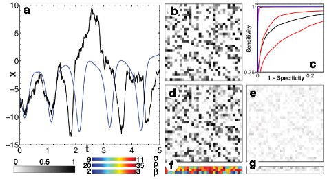
Figure 7: Reconstructing a random network complex chaotic dynamics. Example of $N=32$ Lorenz oscillators with dynamics given by $\dot{x}_{i}=\sigma_{i}(y_{i}-x_{i})+\sum_{j=1}^{N}J_{ij}(x_{j}-x_{i})+\xi_{i}^{(x)},\,\dot{y}_{i}=x_{i}(\rho_{i}-z_{i})-y_{i}+\xi_{i}^{(y)},\,\dot{z}_{i}=x_{i}y_{i}-\beta_{i}z_{i}+\xi_{i}^{(z)}$, with unknown parameters $\forall\,i,j\,\,\{J_{ij},\sigma_{i},\rho_{i},\beta_{i}\}$ in the presence of external Gaussian white noise $\boldsymbol{\xi}_{i}$ of amplitude $\lambda$. (a) Dynamics of a unit in the absence (blue) and presence (black) of noise with $\lambda=5$. Original (b) and reconstructed (c) connectivity, inferred parameters (f), and their errors compared to the original topology and parameters (e) and (g). (c) Receiver operating characteristics (ROC) of reconstruction under noise-free (blue) and noisy measurements (black and red) for $\lambda\in\{0.1,1,10\}$. Figure taken from [12].

It is clear that certain types of dynamics do not allow topology inference. For instance, if all local dynamics are identical $f_{i}\equiv f$, all coupling functions are identical, $g_{ij}\equiv g$, and collectively the units are identically synchronous, i.e. all in the same states at the same times, there is no information about the connection topology one can possibly obtain from (only) recording time series, because for all strongly connected topologies, the collective dynamics would be identical.

Further theoretical considerations show that following the same lines of analysis as above, all parameters occurring linearly in the local dynamics of coupling functions, can also be reconstructed by the same error minimization based on eqn. (11). For instance for the (fictional) coupling function $g_{ij}(x,y)=a\sin(xy)-\exp(b+y-x)$, the parameters $a$ and $b$ need not be known but can be inferred as well (up to one constant prefactor for each pair $(i,j)$ of nodes), because both $a$ and $\exp(b)$ occur linearly in the equations of motions (49). In many physical systems, parameters actually do occur linearly. These include, for instance, the dynamics of coupled classical electric LCR circuits and the strengths of diffusive (4) or direct linear coupling (6). Moreover, widely used model systems for networks of neurons, such as leaky integrate-and-fire and quadratic integrate-and-fire neurons [50] or networks of coupled chaotic systems such as Rössler or Lorenz systems [51, 52] exhibit all or at least most parameters occurring linearly or affinely. For all such systems, local dynamics $f_{i}$ and coupling functions $g_{ij}$ may not or not completely be required to be known in advance.

Such a direct inference method [12] for network topology from complex collective dynamics thus serves as a simple starting strategy for connectivity reconstruction in a broad range of networked systems.

5.2 Pulse-coupling: Reconstruction from spike patterns

Networks of spiking neurons or other pulse-coupled units are formally hybrid systems [53], because the continuous-time flow is interrupted at certain time points, where events (e.g. spike sending or reception) modify the dynamics [54, 55] via discrete time maps.

To start addressing the reconstruction problem for such hybrid systems, researchers have considered one of the simplest model networks of pulse-coupled units based on leaky integrate-and-fire (LIF) models. Such network models are most broadly used in mathematical analysis and computational modeling. Each unit in such a network has one state variable, its membrane potential, roughly emulates leaky capacitive properties observed for membranes of biological neurons and is complemented with a threshold where a pulse (action potential or spike [56]) is artificially created and the membrane potential is reset. Although these models lack certain biological details, such as a natural spike generating mechanisms, they are simple enough to be studied analytically and they have been useful for furthering our understanding how the information is processed among neurons [57].

Explicitly, the membrane potential $V_{i}(t)$ of a LIF unit $i$ changes as in an RC circuit (resistor and a capacitor connected in parallel) according to

$$\dot{V}_{i}=\gamma_{i}(R_{i}I_{i}-V_{i})+S_{i}(t),$$ (52)

where $R_{i}$, $\gamma_{i}$ and $I_{i}$ are the membrane resistance, inverse membrane time constant and the external current applied to neuron $i$, respectively. Once the potential of a unit $j$ crosses a threshold, $V_{j}(t)\geq V_{T,j}$, the potential is reset to $V_{j}(t^{+})=V_{R,j}$ and the unit emits a pulse that it transmitted to the neuron’s post-synaptic neighbors [58]. The time of this pulse sending event is remembered as the unit’s $m$-th spike time $t_{j,m}:=t$. The collection of such pulses then define the actions onto post-synaptic units $i$ such that the quantity

$$S_{i}(t)=\sum_{j=1}^{N}\sum_{k\in\mathbb{Z}}J_{ij}\delta(t-t_{j,m}-\tau_{ij}),$$ (53)

in (52) represents the pulses that unit $i$ receives from the rest of the network. Here, $J_{ij}$ and $\tau_{ij}$ are the synaptic coupling strength and the synaptic transmission delay from unit $j$ and $i$, respectively. Furthermore, $\delta(.)$ is the Dirac delta distribution modeling a potential response kernel that is much faster than all other time scales involved.

The main question we address now is whether and how the network connectivity, as specified by the matrix of coupling strength $J_{ij}$ can be reconstructed if the pattern of spikes times $\left(t_{j,m}\right)_{j\in\{1,\ldots,N\},m\in\mathbb{Z}}$ is given? We remark that we do not assume access to the natural state variables, the membrane potentials $V_{i}(t)$, which may not be observable, but only to the spike times that are generated by the dynamics of these potentials. This difference constitutes the main novelty of the approaches presented in this subsection compared to those for continuous time state variables presented before.

First observe that (52) has an explicit solution [35] given by

$$V_{i}(t)=R_{i}I_{i}(1-e^{-\gamma_{i}(t-t_{0})})+V_{i}(t_{0})e^{-\gamma_{i}(t-t_{0})}+\sum_{j=1}^{N}\sum_{t_{0}<t_{j,m}+\tau_{ij}\leq t}J_{ij}e^{-\gamma_{i}(t-t_{j,m}-\tau_{ij})}.$$ (54)

if the time interval $[t_{0},t)$ lies in between two subsequent spikes of neuron $i$. The first sum is taken over all neurons while the second is taken over those spikes generated by the other neurons $j\neq i$ that affect $i$ in the time interval $[t_{0},t)$.

Based on this solution, we now present two distinct approaches to infer network connectivity, one direct and exact inference method assuming oscillatory units and one coarse approximate method based on stochastic optimization:

5.2.1 Direct topology inference assuming oscillatory units

Van Bussel et al. [35] assumes that all the parameters of (54), besides the synaptic couplings $J_{ij}$, are known. The rationale is that delays and membrane time constants as well as a unit’s equilibrium potential $R_{i}I_{i}$ may be estimated beforehand. How could these coupling strengths and thus the structural network topology be inferred? If the currents $I_{i}$ are sufficiently large such that $R_{i}I_{i}>V_{T,i}$ the units are oscillatory such that they create spike even without recurrent inputs from the remaining network. After crossing the threshold $V_{T,i}$, unit $i$ sends a spike to its post-synaptic neighbors and is reset to a resting value $V_{R,i}$, so that the unit’s state at the boundaries of each inter-spike interval $[t_{i,k-1},t_{i,k})$ is determined and one may take $t_{0}=t_{i,k-1}$ and $t=t_{i,k}$. However, these threshold crossings may be induced in two manners at $t=t_{i,k-1}$, (a) by incoming excitatory spikes from other neurons such that $V_{i}(t^{-})<V_{T,i}$ but $V_{i}(t^{-})+\sum_{\left\{j:\exists m:t_{j,m}+\tau_{ij}=t\right\}}J_{ij}>V_{T,i}$ or (b) by the intrinsic oscillation of the unit such that $V_{i}(t^{-})=V_{T,i}$ without simultaneously incoming spike(s). In both cases, the membrane potential is at reset value immediately after sending a spike. So identifying $t_{0}=t_{i,k-1}$ in (54), we have

$$\begin{array}[]{c}V_{i}(t_{0}):=V_{i}(t_{i,k-1})=V_{R,i}.\end{array}$$ (55)

If the next spike is oscillation-induced (b), the membrane potential approaches its threshold value $V_{T,i}$ continuously such that in addition

$$\begin{array}[]{c}V_{i}(t^{-}):=\begin{array}[]{c}V_{i}(t_{i,k}^{-})=V_{T,i}\end{array}\end{array}$$ (56)

where we now identified $t=t_{i,k}$ in (54). Thus, each oscillation-induced spike at some $t=t_{i,k}$ implies a linear restriction of the form (54) for the coupling strengths $J_{ij}$ by equating $[t_{0},t)=[t_{i,k-1},t_{i,k})$.

For $M$ different inter-spike intervals obeying (55) and (56), this provides a linear system of equations restricting the coupling matrix. However, as van Bussel et al. [35] remark, consecutive intervals may display similar patterns, such that it is often advisable to select $M>N$ inter-spike intervals sufficiently separated in time, to minimize correlations between intervals and thus numerical inaccuracies. For each $i$, defining the subset of inter-spike intervals

$$D_{i,m}:=(t_{i,l_{m}-1},t_{i,l_{m}})$$ (57)

and

$$T_{i,m}=t_{i,l_{m}}-t_{i,l_{m}-1}=|D_{i,m}|$$ (58)

eq. (54) may be rewritten as

$$X_{i}\boldsymbol{J}_{i}^{T}=\boldsymbol{Y}_{i},$$ (59)

where $\boldsymbol{J}_{i}:=(J_{ij})_{j\in\{1,\ldots,N\}}$ and $X_{i}\in\mathbb{R}^{M\times N}$ and $\boldsymbol{Y}_{i}\in\mathbb{R}^{M\times 1}$ are given by

$$\left(X_{i}\right)_{mj}=\sum_{t_{j,k}+\tau_{ij}\in D_{i,m}}J_{ij}e^{-\gamma_{i}(t_{i,l_{m}}-t_{j,k}-\tau_{ij})}$$ (60)

and

$$Y_{i,m}=V_{T,i}-R_{i}I_{i,m}(1-e^{-\gamma_{i}T_{i,m}})-V_{R,i}e^{-\gamma_{i}T_{i,m}}.$$ (61)

Repeating the same process for all units $i$ yields the topology of the whole network. As shown in section 3.2 , the overdetermined problem, $M>N$, and the undetermined, $M\ll N$, may be solved minimizing the $L_{2}$-norm or maximizing the sparseness of the network, respectively. A major limitation is that the presented approach requires a large amount of prior knowledge about the system, such as the time delays between units and their time constants, among others. Given this knowledge, the approach is capable of inferring large networks of neurons as the computation time, as well as the number $M$ of required inter-spike intervals to be evaluated scales linearly with system size [35, 59].

5.2.2 Stochastic optimization of all systems parameters

In a complementary study, Makarov et al. [60] showed how stochastic optimization of all system parameters

$$\boldsymbol{p}_{i}=\left(\gamma_{i},R_{i},I_{i},\tau_{ij},J_{ij}\right)_{i,j\in\{1,\ldots,N\}}$$ (62)

given the spike trains for all neurons in the network may yield a network topology roughly consistent with the actual one.

The idea is to evaluate the predicted inter-spike interval durations $\bar{T}_{i,m}(\boldsymbol{p})$ from a test set of parameters and to optimize those parameters to reproduce a given (measured) spike train as closely as possible. Thus, minimizing the difference between the predicted and measured spike trains is vital for this method. The authors in particular applied their idea also to recordings of biological neurons.

As the eq. (54) yields transcendental relations for the $\bar{T}_{i,m}(\boldsymbol{p})$, their estimates need to be determined numerically. Thus, finding

$$\boldsymbol{p}_{i}^{*}=\arg\min_{\boldsymbol{p}_{i}}\,E_{i}(\boldsymbol{p}_{i})=\arg\min_{\boldsymbol{p}_{i}}\sum_{m=1}^{M}(T_{i,m}-\bar{T}_{i,m}(\boldsymbol{p}_{i}))^{2}$$ (63)

yields the best (in Euclidean distance norm) solution for the set of parameters.

Briefly, to find the minimum $\boldsymbol{p}_{i}^{*}$ in (63) one must explore the parameters space. This means that the solution is found through iteratively choosing random values for $\boldsymbol{p}_{i}$ and comparing the value of (63) for consecutive iterations. By relating the changes in (63) with the changes in $\boldsymbol{p}_{i}$ one may establish directions in which the minimum may be found by gradient descent. However, it is also advisable to change directions in the parameters space randomly. Mainly, because there may better solutions for $\boldsymbol{p}_{i}^{*}$ in regions of the parameters space where they are not expected to exist [61]. Makarov et al. [60] thus applied stochastic optimization for searching the minimum.

As a strong requirement, this method needs that the number of recorded spikes to be $M$$\gg 2N$; as noted in [60], robust regression models are more suitable to handle this kind of problems and special care with the inter-spike intervals must be taken as, e.g., spike bursts may lead to false intervals.

5.3 Features and limitations

The stochastic optimization approach provides a generic approach in finding best fitting parameters and thus here, potentially a well fitting network; yet, it is computationally demanding and simultaneously requires many recordings compared to the size of the network. In contrast, the direct approach assumes a large amount of pre-knowledge, in particular regarding the unit’s parameters. In addition, by requiring to pre-process the data sets (i.e. choosing appropriate time intervals), the minimization problem is no longer required to deal with transcendental relations. This leads to a considerable increase on the computational performance and it is the key factor that makes the method suitable for large networks. We remark that still, both methods are currently not suitable in our opinion to reliably infer network topology from real recordings of spike data, because of several reasons: For instance, other network-external sources of spike generation, stochastic fluctuations due to intrinsic noise and the highly specific conditions required for reconstruction still limit the methods applicability. Finally, both approaches assume linearity of interactions, yet it is known that interactions can be nonlinear, e.g. due to dendritic spikes in response to sufficiently strong, simultaneous inputs to single dendritic branches of a neuron [62, 63, 64].

6 Technical issues

Let us briefly comment on four technical issues related to the structural inference approaches discussed above. We mention how some of them may be directly transferred to settings, where discrete time dynamics describes the system (section 6.1), discuss issues when measuring data from real, e.g. biological networks (section 6.2), remark on $L_{1}$ vs. $L_{2}$ minimization (section 6.4) and finally discuss what happens for hyper-networks, where more than two-point interactions influence the collective state (section 6.5).

6.1 Discrete time maps

If the dynamical system is described as a network of coupled discrete-time maps instead of by coupled differential equations (2), approaches similar to the ones presented above are often viable in slightly modified form. For instance, the core equation becomes (for 1-dimensional local units)

$$\boxed{x_{i}(t+1)=f_{i}\left(x_{i}(t)\right)+\sum_{j=1}^{N}J_{ij}g_{ij}\left(x_{i}(t),x_{j}(t)\right)+I_{i}(t)+\xi_{i}(t)}$$ (64)

where now the time $t\in\mathbb{Z}$ is an integer. Here, the direct method of subsection 5.1 is immediately applicable, even with the additional advantage that no temporal derivatives need to be estimated such that an observed time series $(x_{i}(t))_{i\in\{1,\ldots,N\},t\in\{1,\ldots,M\}}$ enters the inference equations without approximations. Of course, that time series may still contain substantial measurement errors that propagate into any solution of the inference problem.

6.2 Sampling dynamics of real networks

When sampling real life phenomena, measurement constraints may arise due to the nature of the given phenomena, making the study of such a major challenge. For instance, in EEG analysis, a group of sensors is employed to measure the brain activity. These recordings help in finding functional connections among regions in the brain. Basically, each sensor measures the activity of a population of neurons below its active area for a certain amount of time. Then, by analyzing the correlations among the time series of each sensor, the interaction network is constructed. Nevertheless, as remarked by Bialonski in [65], special considerations regarding the spatial and temporal sampling must be accounted for. A simple constraint is that sensors placed too close to each other, may record overlapping activity from neighboring populations, thus increasing the difficulty to discern between direct and indirect interactions. Moreover, if the size and frequency of the sampling fails to capture the intrinsic time scales, false functional connections in network may be constructed. Clearly this example is particularly relevant for inferring effective connectivities, as discussed in section 7. As an example regarding the time domain, gene and protein interaction networks often still have a very limited number of sampling points available [66, 67] such that a network inference problem may become drastically under-determined. Additional information such as the known existence of certain interactions in such a network (but not the existence of others) sometimes is available but how precisely to use this is currently unknown and requires further method development. So briefly, when studying real networks, special technical considerations should be accounted for to actually use what it is measured (the data) for what one wants to know about the system, cf. section 1.2.

6.3 $L_{1}$ norm minimization as a linear program

Given the optimization problem

$$\min_{\boldsymbol{y}}\left\|A\boldsymbol{y}-\boldsymbol{b}\right\|_{1},$$ (65)

where $A\in\mathbb{R}^{M\times N}$, $\boldsymbol{y}\in\mathbb{R}^{N}$ and $\boldsymbol{b}\in\mathbb{R}^{M}$, (65) may be posed as [31]

$$\min_{\boldsymbol{s}}\boldsymbol{1}^{\mathsf{T}}\boldsymbol{s}\quad\text{s.t. }\begin{array}[]{c}A\boldsymbol{y}-\boldsymbol{b}\preceq\boldsymbol{s}\\ A\boldsymbol{y}-\boldsymbol{b}\succeq-\boldsymbol{s}\end{array},$$ (66)

where $\boldsymbol{1}\in\mathbb{R}^{M}$ is a vector of ones and $\preceq$ and $\succeq$ denote entry-wise comparison and $\boldsymbol{s}$ is an auxiliary variable. To solve (66), one has to solve the linear program

$$\min_{x}\tilde{\boldsymbol{c}}^{\mathsf{T}}\boldsymbol{x}\text{\quad\text{s.t.}}\quad\tilde{A}\boldsymbol{x}=\tilde{\boldsymbol{b}},$$ (67)

where

$$\boldsymbol{x}=\left[\begin{array}[]{c}\boldsymbol{y}\\ \boldsymbol{s}\end{array}\right],\quad\tilde{A}=\left[\begin{array}[]{cc}A&-I\\ -A&-I\end{array}\right],\quad\tilde{\boldsymbol{b}}=\left[\begin{array}[]{c}\boldsymbol{b}\\ -\boldsymbol{b}\end{array}\right],\quad\tilde{\boldsymbol{c}}=\left[\begin{array}[]{c}\boldsymbol{0}\\ \boldsymbol{1}\end{array}\right]$$ (68)

and $I\in\mathbb{R}^{M\times M}$ and $\boldsymbol{0}\in\mathbb{R}^{N}$ are the identity matrix and a vector of zeroes, respectively. The advantage of posing problem (65) as (67) is that the latter can be easily solved in a standard way by implementing any solver for linear programs (e.g. the linprog function in MATLAB [32]).

6.4 $L_{2}\,\text{\,\ vs.\,\,\ $L_{1}$}$ norm minimization

The need to choose a minimization scheme may turn the reconstruction problem into a great challenge, because different schemes may yield different solutions, thus forcing us to discern which scheme is best suited for our purposes in specific reconstruction problems. As illustrated in [1, 10, 60, 68, 59, 35, 29] these differences between minimizers may be exploited in certain situations. For instance, the $L_{2}$ minimizer finds the closest solution in the $L_{2}$-norm and moreover has an analytic solution. Yet, given the nature of the minimizers (check [68]), an $L_{1}$ minimizer is suited for finding particular sparse solutions and it is more robust to outliers than $L_{2}$, so it might be seen as more useful for applications. However, minimizing an $L_{1}$ norm is computationally more costly compared to the $L_{2}$ and it may have more than one solution [31]. We note that $\left\|\boldsymbol{p}\right\|_{2}\leq\left\|\boldsymbol{p}\right\|_{1}$ for any vector $\boldsymbol{p}\in\mathbb{R}^{N}$

6.5 Hypernetworks: beyond two-point interactions

We have explicitly excluded networks with more than two-unit interactions from our general mathematical description (2) or dynamical networks with temporally changing connections. Those may occur, for instance in networks of computers, or other communication networks of engineering, where inputs from several units that give input to the same other unit are nonlinearly processed (for instance, multiplied) to change the latter units’ state. Similarly, non-additive dendritic interactions in neurons [63, 20], where two simultaneously received synaptic inputs in close spatial proximity initiate so-called dendritic spikes and thereby a nonlinearity [62], naturally imply three-point interactions.

We remark that direct three-unit and higher order interactions (i.e. three-term and higher order products such as $x_{i}^{d}x_{j}^{d^{\prime}}x_{k}^{d"}$ where $i,j,k$ are mutually different) are omitted in (1) because they refer to dynamical systems on hypernetworks, thus going beyond the scope of this review. Such third order and higher order terms are not covered by (1), firstly, because the notation stays much simpler without them, but secondly and more importantly, because there seem to be few major theoretical results on reconstructing such systems, if any, that may be or become of practical use. Yet, in social, communication and information networks, such questions may soon become of interest as ’big data’ are pouring in.

A brief introduction to the dynamics of complex hypernetworks is given in [17].

7 Effective connectivity: Correlation-based methods

7.1 Linear correlation and covariance

One common way of quantifying effective connectivity is to measure scalar time series $\boldsymbol{x}(t)=(x_{1}(t),\ldots,\,x_{N}(t))$, $t\in\{t_{1},\ldots t_{M}\}$ from the $N$ units of a system (spike rates of neurons, expression levels of genes, …), compute their (temporal) averages $\mu_{i}=\left\langle x_{i}(t)\right\rangle_{t}$ and variances $\sigma_{i}^{2}=\left\langle\left(x_{i}(t)-\mu_{i}\right)^{2}\right\rangle_{t}$ and from those compute the covariance matrix

$$\mbox{Cov}_{ij}:=\frac{\left\langle\left(x_{i}(t)-\mu_{i}\right)\left(x_{j}(t)-\mu_{j}\right)\right\rangle_{t}}{\sigma_{i}\sigma_{j}}.$$ (69)

Here the averages are time averages

$$\left\langle y_{i}(t)\right\rangle_{t}:=M^{-1}\sum_{m\in\{1,\ldots,M\}}y_{i}(t_{m}).$$ (70)

If multiple measurements are available, averages may be taken over ensembles of experiments rather than (or in addition to) temporal averaging. The obtained covariance matrix is then often thresholded, either just choosing a heuristic value or according to some measure of statistical significance (against an appropriate null hypothesis) and the resulting non-zero values interpreted either as “strength” of effective connectivity (weighted connectivity matrix) or just as existence (adjacency matrix) of a functional link between units. Sometimes, the value of a threshold is systematically varied and changes in resulting connectivity evaluated. Correlation, covariance and other linear algebra measures are commonly used, often complemented by nonlinear operations such as thresholding, to analyze, for instance fMRI or other spatio-temporal data [69]. We note that correlation measure may be (mathematically) seen in a number of different ways [70].

7.2 Entropy maximization

Entropy measures the uncertainty associated with a given probability distribution and constitutes a key quantity in information theory [71] . Given the probabilities of a set of events, the entropy measures how uncertain, on average, the occurrence of an event is; or in other words, how much information, on average, one obtains by measuring the occurrence of that event knowing the probability distribution of events. Reversely, given a collection of (observed) data points, we can choose probabilities to maximize the entropy. Such a distribution, known as a maximum-entropy probability distribution, would be the least biased distribution possible and any other would require further assumptions on the nature of the problem [72]. For a network dynamical system, i.e. systems of coupled dynamical units, we can ask what the effective interactions are such that the probability distribution that best describes the data (averages and correlations) has maximum entropy.

Specifically, the principle of maximum information from Bayesian statistics postulates the “most likely” probability $\rho(\boldsymbol{x})$ of measuring $\boldsymbol{x}$ given the same type of time series data $\boldsymbol{x}(t)=(x_{1}(t),\ldots,\,x_{N}(t))$ is the one maximizing the information obtained from measuring one more state $\boldsymbol{y}$. More precisely, the goal is to find the probability $\rho(\boldsymbol{x})$ that maximizes Shannon entropy

$$S=-\sum_{\boldsymbol{x}}\rho(\boldsymbol{x})\ln\rho(\boldsymbol{x})$$ (71)

under the constraints that the first and second moments are consistent with those estimated from the data,

$$\left\langle x_{i}\right\rangle_{\rho}:=\sum_{\boldsymbol{x}}x_{i}\rho(\boldsymbol{x})\overset{!}{=}\left\langle x_{i}(t)\right\rangle_{t}$$ (72)

and

$$\left\langle x_{i}x_{j}\right\rangle_{\rho}:=\sum_{\boldsymbol{x}}x_{i}x_{j}\rho(\boldsymbol{x})\overset{!}{=}\left\langle x_{i}(t)x_{j}(t)\right\rangle_{t}$$ (73)

By restricting ourselves to these conditions (and no others), we here focus on pairwise interactions and neglect three-point and higher order coupling that arise in hypernetworks (cf. section 6.5 and [17]). This yields (Appendix A) the probability distribution of the form

$$\rho(\boldsymbol{x})=Z^{-1}\exp\left(\sum_{i=1}^{N}h_{i}x_{i}+\frac{1}{2}\sum_{i=1}^{N}\sum_{j=1}^{N}\hat{J}_{ij}x_{i}x_{j}\right)$$

where $Z=\int_{\mathbb{R^{N}}}\exp\left(\sum_{i=1}^{N}h{}_{i}x_{i}+\frac{1}{2}\sum_{i=1}^{N}\sum_{j=1}^{N}\hat{J}_{ij}x_{i}x_{j}\right)d^{N}x$ is a normalization constant and $h_{i}$ and $\hat{J_{ij}}$are parameters to be chosen such that (88) and (89) hold. The quantities $\hat{J}_{ij}$ are interpreted as effective couplings between units $i$ and $j$.

If the matrix of covariances between the $N$ time series is

$$C_{ij}=\left\langle x_{i}(t)x_{j}(t)\right\rangle_{t}-\left\langle x_{i}(t)\right\rangle_{t}\left\langle x_{j}(t)\right\rangle_{t}\,.$$ (74)

the effective coupling matrix is given by its inverse (Appendix A)

$$\hat{J}=C^{-1}.$$ (75)

This means that the best available probability distribution (i.e. that yielding the maximum information) is given by second order effective coupling strengths determined by (but by no means identical to) the linear correlation matrix.

This concept is applied to a range of different systems, in particular in biology, including gene networks [73], protein networks [74] and neural circuits [75]. We comment on an approach originally suggested by Bialek and coworkers [75, 76] for revealing in how far two-point interactions characterize the coupled dynamics of neural circuits in retina. In fact, a systematic study of neural activity in the retina of larval tiger salamander and guinea pig revealed that $90\%$ of the multi-information (which measures all correlative dependencies in a system [76]) is covered by pairwise correlations only [75]. The authors took this finding as a sign that pairwise interactions well characterize the full network dynamics and that higher order interactions may be neglected. Specifically, they temporally discretized neural responses into “1” or “0” states depending on whether a neuron was or was not active during each considered time interval of generically $20\,\mbox{ms}$. Thus, the state of the entire (observed) network at each time interval is given by an $N-$dimensional word composed of the binary components of the $N$ neurons. As sometimes done for effective connectivity, researchers often tend to go beyond what Bialek and coworkers concluded and interpret the effective coupling strengths (75) as actual physical interactions of experimentally observed units. However, it is typically not clear how correlative dependencies yield information about direct physical interactions and such that such interpretations are not justified without substantial further knowledge about the system.

7.3 Further in finding effective connectivity

We would like to emphasize that there is a multitude of additional approaches for finding effective or functional connectivities. For instance, a range of methods are based on information theoretic measures such as mutual information [77], transfer entropy [78] and Granger causality [79, 80] and extensions thereof. In addition, there are various methods relying on Bayesian statistics or explicit or implicit modeling or extended regression such as used in generalized linear models [81]. In particular in biological sciences, such statistical methods have been used early on even at times not many or not very reliable data were available, see for instance [82] for an early study regarding effective connectivity in neural circuits.

There are a number of open challenges regarding both precision of such methods and the interpretation of the respective results. For instance, functional magnetic resonance imaging (fMRI) experiments of brain areas may rely on differences in blood oxygen level (so-called BOLD signals) as observables but often aims to relate actual dependencies in neural spiking activity. The reasoning here is that the cell metabolism and thus the blood oxygen consumption in a local region (typically one cubic millimeter) of the brain is larger the more action potentials per time are generated by the ($10^{4}-10^{6}$) neurons in that region so that such approaches are not undisputed [83]. Moreover, the terms effective connectivity, functional connectivity and structural or anatomical connectivity are sometimes not well defined, used in different meanings across studies. There are even overlapping definitions of non-structural forms of connectivity, e.g. for functional connectivity, effective connectivity etc. Here we did not delve into historic waters and used the term “effective connectivity” for all forms of connectivity that is not structural. Sometimes, effective connectivity is even taken as an indication for structural connectivity of physical interactions. For instance, distinguishing direct interactions from indirect influences may be an important issues (cf. Fig. 1) that is not yet fully clarified [84].

Finally, we mention that for neural circuits [85] have devised a statistical method to find the couplings $J_{ij}$ that optimize the likelihood that a class of integrate and fire models generates the spike trains observed in experiments. This statistical method assumes the same model class as the approach for inferring structural connectivity presented above (section 5.2) and its goal indeed is finding the (most likely) structural connectivity.

As a conclusive warning, we remark that in particular different methods exit for obtaining effective connectivity given the same data set; the results each provide information about specific features of the system: exactly those defined by the method. Some might almost coincide with others, some might be congruent with and some may well be contradicting a given structural connectivity (cf. [86]).

8 Conclusion and Open Questions

This review focuses on how structural connectivity of networks may be inferred from dynamical features of the networks’ nodes. It is on purpose on an introductory level and (given that the area of network reconstruction is rapidly growing simultaneously in different fields, from gene and neural networks to engineering systems) by construction only highlights some selected approaches, most of which based on a perspective of considering the collective nonlinear network dynamics. We provide basic approaches about finding effective or functional connectivities of a network from time series as a brief complement and to get a taste for essential differences in perspective. One main distinction between approaches for identifying qualitatively different types of connectivity is that structural inference, aiming to reconstruct real physical interactions, take into account the time evolution of a system. In contrast, finding effective connectivity is often based on a stationarity assumption and uses distributions of states, neglecting all or parts of their temporal evolution. Relating observable, possibly effective and physical connectivity, is at the heart of current interdisciplinary research [15, 87]. As also mentioned in the Introduction and briefly discussed in section 7, functional vs. structural inference if often not well distinguished and, in particular in early publications, the qualitative difference in approach was sometimes not even mentioned.

The methods and approaches presented in this review aim to tell whether or not and how strongly units in a network directly interact with each other. This is in distinction to the entire field of system’s identification [7] where the aim is to identify the rules underlying a dynamical system from time series and predict its (future) dynamics based on this identification. Systems identification for multi-dimensional systems, and thus in particular for large networks, seems intractably hard because even if the “real” system is almost (but not entirely) perfectly reconstructed, predicting their future dynamics can be impossible due to chaos (sensitive dependence on initial conditions), exponentially many different collective states and uncontrolled external influences, with all these factors becoming typical for multi-dimensional complex systems. At the same time, as in part illustrated in this review Figure 5, learning the existence of strengths of interactions only (and not the precise form of dynamics) may well be successful for much larger systems. We thus speculate that novel methods complementing those of systems identification may yield further insights into the interaction networks of various complex systems.

A number of key issues are not discussed in this review but still are sometimes pressing for progress research, in particular with respect to applications to real world settings. We list a few:

1. How much information can we actually access (cf. [88])? Can we observe all the units of a network? Can we observe all dynamical variables (dimensions) of each unit? In which sense may it make sense to seek connectivity of nodes that are not observed?

2. What do we know a priori about the system? Are the functional forms of network interactions known? What can we say about stability or instability of the dynamics? Perhaps the dynamics even exhibits a complex mixture of stable and unstable dynamics [9, 89, 90].

3. What are reasonable (or possible) number of experiments or measurements that can be done and what is a clever trade-off against the required computational efforts that may depend on the quality and quantity of those measurements [23].

4. Which of the structural features are actually the most relevant and which are even possible. In biochemical and gene regulatory networks, electric circuits and power grids, for instance, many interaction links (or their absence) may have been identified by other methods not related to network collective dynamics. Under these circumstances, can we improve existing approaches to take such information into account?

5. How can we address genuinely stochastic dynamics, e.g. in excitable systems, possibly even induced by small number fluctuations – a pathway of though that links to non-equilibrium physics, cf. [91]?

6. What if network connectivities change, for instance by synaptic plasticity in neural circuits [92, 93, 94] or other forms of adaptation, e.g. in social networks [95].

7. … think of your own, there are many more questions with great opportunity for scientific progress in a range of fields …

Answers to all these questions will specifically restrict or enhance the space of optional networks consistent with recorded data. From an abstract point of view, these modify the form and dimensionality of the set of all possible networks and points to a direction that still addresses network dynamics as an inverse problem but goes beyond network reconstruction. Given all restrictions, perhaps we can design or control a network to robustly exhibit a specific functionality. Network design and control form two additional branches in the theory of network dynamical systems, with currently highly active research, from biological sciences to engineering [11, 96, 97, 98, 99]. Such approaches might soon be extremely influential and thought-provoking, when, e.g., the neural and biochemical networks in our bodies as well as our infrastructure networks surrounding us can not only be reconstructed, but even controlled and specifically engineered. We recommend a view point by Freeman Dyson for a very practical taste [100].

Acknowledgements: We thank Srinivas Gorur Shandilya for help during project initiation and Raoul-Martin Memmesheimer, Mor Nitzan, Dirk Witthaut, David Gross, Matthias Wendland, Sarah Hallerberg and Hinrich Arnoldt for valuable discussions and constructive comments on parts of the manuscript. Partially supported by the International Max Planck Research School (IMPRS) Physics of Biological and Complex Systems (JC) the Ministry for Education and Science (BMBF), Germany, through the Bernstein Center for Computational Neuroscience, grant number 01GQ1005B (MT) as well as by a grant by the Max Planck Society to MT.

Appendix A Multiple Linear Regression and $L_{2}-$Norm Minimization

Multiple linear regression is a widely-used statistical tool for predicting values of a set of variables depending on one independent set of variables. Its main purpose is to infer a linear relationship between them. Thus, the relationship between sets is assumed to have the form

$$\boldsymbol{y}=\boldsymbol{\text{$\boldsymbol{\beta}$}}x+\text{$\boldsymbol{\varepsilon}$},$$ (76)

where $\boldsymbol{y}\in\mathbb{R}^{1\times M}$ are the values for a dependent variable, $\boldsymbol{\boldsymbol{\beta}}\in\mathbb{R}^{1\times K}$ the column vector of unknown linear coefficients, $x\in\mathbb{R}^{K\times M}$ is the set of values for the $K-$independent variables and $\boldsymbol{\boldsymbol{\varepsilon}}=(\varepsilon_{1},\ldots,\varepsilon_{M})\in\mathbb{R}^{1\times M}$ are random errors $\varepsilon_{i}$, $i\in\{1,\ldots,M\}$. In addition, the errors $\varepsilon_{i}$ are assumed to be independent random variables distributed according to a Gaussian distribution with mean $\mu=0$ and constant variance $\sigma^{2}$ [101].

The question is how to estimate $\boldsymbol{\beta}$ by some $\hat{\boldsymbol{\beta}}$ such that the difference between the predicted and real values, $\boldsymbol{\text{$\boldsymbol{\beta}$}}x$ and $\boldsymbol{y}$, is minimized? Using $L_{2}$ minimization, the problem formally becomes

$$\hat{\boldsymbol{\beta}}=\arg\min_{\boldsymbol{\beta}}\|\boldsymbol{y}-\boldsymbol{\beta}x\|_{2}^{2},$$ (77)

also known as the linear least squares method [101].

The local extremum of the $L_{2}$ norm appearing in the right hand side of (77) implies

$$\forall i\in\{1,\ldots,K\}\,:\,\,\,\left.\dfrac{\partial}{\partial\beta_{i}}\left[(\boldsymbol{y}-\boldsymbol{\beta}x)(\boldsymbol{y}-\boldsymbol{\beta}x)^{T}\right]\right|_{\boldsymbol{\beta}=\boldsymbol{\hat{\beta}}}=0.$$ (78)

such that

$$\left.\dfrac{\partial}{\partial\beta_{i}}\left[\boldsymbol{yy}^{T}-2\boldsymbol{\beta}x\boldsymbol{y}^{T}-\boldsymbol{\beta}x(\boldsymbol{\beta}x)^{T}\right]\right|_{\boldsymbol{\beta}=\boldsymbol{\hat{\beta}}} = 0,$$

$$\Leftrightarrow\left.\dfrac{\partial\boldsymbol{\beta}}{\partial\beta_{i}}\left(x\boldsymbol{y}^{T}-x(\boldsymbol{\beta}x)^{T}\right)\right|_{\boldsymbol{\beta}=\boldsymbol{\hat{\beta}}} = 0,$$

which in turn implies the best estimate

$$\hat{\boldsymbol{\beta}}=\boldsymbol{y}x^{T}(xx^{T})^{-1},$$ (79)

of $\boldsymbol{\beta}$ according to the linear least squares method [101].

Appendix B Singular Value Decomposition and $L_{1}-$Norm Minimization

Singular Value Decomposition (SVD) is regarded as an important tool for statisticians due to its broad variety of applications (reduced rank regression, polar decomposition, image compression, among others [102]). Formally, from the fundamental theorem of linear algebra, any rectangular matrix $A\in\mathbb{R}^{m\times n}$ may be decomposed into the product of three matrices as

$$A=U\Sigma V^{\mathsf{T}},$$ (80)

where $U\in\mathbb{R}^{m\times m}$ and $V\in\mathbb{R}^{n\times n}$ are unitary matrices with their columns referred to as left and right singular vectors, respectively, and $\Sigma\in\mathbb{R}^{m\times n}$ is a rectangular diagonal matrix containing the singular values [103]. This decomposition is known as the Singular Value Decomposition of matrix $A$.

The SVD properties are useful in finding the set of all possible solutions to an under-determined system of equations, because for every under-determined system

$$A\boldsymbol{y}=\boldsymbol{b},$$ (81)

where $\boldsymbol{b}\in\mathbb{R}^{m\times 1}$, we can use SVD (80) to rewrite $A$ such that solving (81) for $\boldsymbol{y}$ yields the particular solution

$$\boldsymbol{y}_{p}=V\tilde{\Sigma}U^{\mathsf{T}}\boldsymbol{b},$$ (82)

where $\tilde{\Sigma}\in\mathbb{R}^{n\times m}$ is the pseudo-inverse of $\Sigma$ and is defined as

$$\tilde{\Sigma}=\Sigma^{\mathsf{T}}\left(\Sigma\Sigma^{\mathsf{T}}\right)^{-1}.$$ (83)

Equation (82) defines a particular solution from the set of all possible solutions. The general solution to equation (81) is given by our particular solution plus a linear combination of vectors in the null-space of $A$, i.e.,

$$\boldsymbol{y}=V\tilde{\Sigma}U^{\mathsf{T}}\boldsymbol{b}+V\boldsymbol{c},$$ (84)

where $\boldsymbol{c}\in\mathbb{R}^{n\times 1}$ and $c_{i}=0$ for $i\in\{1,...,r\}$ and $r=Rank(A)$. The latter ensures that the linear combinations are made only with vectors that span the null-space.

In this case, the problem consists in maximizing the number of zero entries in $\boldsymbol{y}$ by choosing the $c_{j}\,\,\forall\,\,j>r$ properly. This may be achieved by solving the overdetermined system (84) with $M$ equations and $M-r$ unknowns. Specifically, it has been illustrated in [10, 29, 35] that by solving

$$\arg\min_{\boldsymbol{y}}\|V\tilde{\Sigma}U^{T}\boldsymbol{b}+V\boldsymbol{c}\|_{1},$$ (85)

employing the Barrowdale and Roberts algorithm [34], a solution having a low number (possibly the least number) of non-zero values, consistent with the restricting equations, is often recovered. However, there seem to not be a general proof of this observation [31]. In the network reconstruction context, it has been shown that optimizing systems like (85) (where $\boldsymbol{y}$ and $\boldsymbol{b}$ are replaced by the unit’s connectivity $\boldsymbol{J}_{i}^{\mathsf{T}}$ and network constraints $\boldsymbol{Y}_{i}^{\mathsf{T}}$) yields the actual network topology when the network is sparse (even if there are less linear constraints than units in the network).

Appendix C Estimating maximum entropy parameters.

Maximizing the entropy

$$S[\rho]:=-\sum_{\boldsymbol{x}}\rho(\boldsymbol{x})\ln\rho(\boldsymbol{x}),$$ (86)

we derive first the functional form of $\rho(\boldsymbol{x})$ and second its parameters under the constraints that the non-negative function $\rho\geq 0$ is normalized

$$\sum_{\boldsymbol{x}}\rho(\boldsymbol{x})=1,$$ (87)

and the first moment

$$\left\langle x_{i}\right\rangle_{\rho}:=\sum_{\boldsymbol{x}}x_{i}\rho(\boldsymbol{x})\overset{!}{=}\left\langle x_{i}(t)\right\rangle_{t},$$ (88)

and second moment

$$\left\langle x_{i}x_{j}\right\rangle_{\rho}:=\sum_{\boldsymbol{x}}x_{i}x_{j}\rho(\boldsymbol{x})\overset{!}{=}\left\langle x_{i}(t)x_{j}(t)\right\rangle_{t},$$ (89)

are consistent with those estimated from data of $N$ time scalar series $x_{i}(t)$. The covariance matrix is defined via the data as

$$C_{ij}=\left\langle x_{i}(t)x_{j}(t)\right\rangle_{t}-\left\langle x_{i}(t)\right\rangle_{t}\left\langle x_{j}(t)\right\rangle_{t}\,.$$ (90)

We maximize the entropy under these $1+N+N(N-1)/2$ constraints using a Lagrange function

$$L[\rho]:=S[\rho]-a\sum_{\boldsymbol{x}}\rho(\boldsymbol{x})-\sum_{i=1}^{N}h_{i}\sum_{\boldsymbol{x}}x_{i}\rho(\boldsymbol{x})-\frac{1}{2}\sum_{i=1}^{N}\sum_{j=1}^{N}\gamma_{ij}\sum_{\boldsymbol{x}}x_{i}x_{j}\rho(\boldsymbol{x}),$$ (91)

where we drop constants as they do not influence the location of a maximum. Here $a$, $h_{i}$ and $\frac{1}{2}\gamma_{ij}$ are the Lagrange multipliers to be determined. Computing the first derivatives and equating them to zero

$$-\frac{\partial L}{\partial\rho(\boldsymbol{y})}=\ln\left(\rho(\boldsymbol{y})\right)+1+a+\sum_{i=1}^{N}h_{i}y_{i}+\frac{1}{2}\sum_{i=1}^{N}\sum_{j=1}^{N}\gamma_{ij}y_{i}y_{j}\overset{!}{=}0,$$ (92)

yields the (unique local) maximum entropy of the form

$$\begin{array}[]{rcl}\rho(\boldsymbol{x})&=&\exp\left(-1-a-\sum_{i=1}^{N}h_{i}x_{i}-\frac{1}{2}\sum_{i=1}^{N}\sum_{j=1}^{N}\gamma_{ij}x_{i}x_{j}\right)\\ &=&\exp\left(-1-a-\boldsymbol{h}^{\textsf{T}}\boldsymbol{\boldsymbol{x}}-\frac{1}{2}\boldsymbol{x}^{\textsf{T}}\hat{J}\boldsymbol{x}\right)\\ &=&A\exp(-\frac{1}{2}\boldsymbol{z}^{\textsf{T}}\hat{J}\boldsymbol{z})\end{array},$$ (93)

where we use the abbreviations $\hat{J}:=\left(\gamma_{ij}\right)_{ij}$, $\boldsymbol{z}:=\boldsymbol{x}+\hat{J}^{-1}\boldsymbol{h}$ is an affine function of $\boldsymbol{x}$ and

$$A:=\exp\left(-1-a+\frac{1}{2}\boldsymbol{h}^{\textsf{T}}\hat{J}^{-1}\boldsymbol{h}\right),$$ (94)

is independent of $\boldsymbol{x}$.

In summary, this exact computation yields the probabilities of the form

$$\rho(\boldsymbol{x})=Z^{-1}\exp\left(\sum_{i=1}^{N}h_{i}x_{i}+\frac{1}{2}\sum_{i=1}^{N}\sum_{j=1}^{N}\hat{J}_{ij}x_{i}x_{j}\right),$$ (95)

where $Z^{-1}=\exp\left(-1-a\right)$.

To estimate the parameters $a$, $h_{i}$ and $\hat{J}_{ij}$ we make the approximation that the data $\boldsymbol{x}_{i}$ form a continuous set such that we can approximate sums by integrals. We then first observe that

$$\sum_{\boldsymbol{x}}\rho(\boldsymbol{x})\overset{\mathsf{cont}}{=}\int_{\mathbb{R}^{N}}\rho(\boldsymbol{x})d^{N}x=\int_{\mathbb{R}^{N}}Ae^{-\frac{1}{2}\boldsymbol{z}^{\textsf{T}}\hat{J}\boldsymbol{z}}d^{N}z\overset{!}{=}1,$$ (96)

due to normalization (87). This implies

$$A=(|\det(\hat{J})|/(2\pi))^{N/2},$$ (97)

and thus yields the parameter $a$ as a function of $\boldsymbol{h}$ and $\hat{J}$. Similarly, fixing the averages (88) yields (approximately)

$$\begin{array}[]{rcl}\left\langle x_{i}\right\rangle&=&\int_{\mathbb{R}^{N}}\,x_{i}\rho(\boldsymbol{x})d^{N}x\\ &=&\int_{\mathbb{R}^{N}}Ae^{-\frac{1}{2}\boldsymbol{z}^{\textsf{T}}\hat{J}\boldsymbol{z}}\left(z_{i}-\sum_{j=1}^{N}\hat{(J^{-1})}_{ij}h_{j}\right)d^{N}z\\ &=&\sum_{j=1}^{N}(\hat{J}^{-1})_{ij}h_{j}\end{array},$$ (98)

for all $i$ and thus $\boldsymbol{h}$ as a function of $\hat{J}$.

Finally, the equations fixing the second moments

$$\begin{array}[]{rcl}\left\langle x_{i}x_{j}\right\rangle&=&\int_{\mathbb{R}^{N}}\,x_{i}x_{j}\rho(\boldsymbol{x})d^{N}x\\ &=&\int_{\mathbb{R}^{N}}x_{i}x_{j}\exp\left(-1-a-\boldsymbol{h}^{\textsf{T}}\boldsymbol{\boldsymbol{x}}-\frac{1}{2}\boldsymbol{x}^{\textsf{T}}\hat{J}\boldsymbol{x}\right)d^{N}x\end{array},$$ (99)

can be evaluated using

$$F(\boldsymbol{h},\boldsymbol{x})=\exp\left(-1-a-\boldsymbol{h}^{\textsf{T}}\boldsymbol{\boldsymbol{x}}-\frac{1}{2}\boldsymbol{x}^{\textsf{T}}\hat{J}\boldsymbol{x}\right),$$ (100)

subjected to

$$\frac{\partial^{2}F}{\partial h_{i}\partial h_{j}}=x_{i}x_{j}F(\boldsymbol{h},\boldsymbol{x}).$$ (101)

With the transformation $\boldsymbol{x}=\boldsymbol{z}-\hat{J}^{-1}\boldsymbol{h}$, eqn. (99) becomes

$$\begin{array}[]{rcl}\left\langle x_{i}x_{j}\right\rangle&=&\frac{\partial^{2}}{\partial h_{i}\partial h_{j}}\,\int_{\mathbb{R}^{N}}F(\boldsymbol{h},\boldsymbol{x})\,d^{N}x\\ &&\frac{\partial^{2}}{\partial h_{i}\partial h_{j}}\,\exp(\frac{1}{2}\boldsymbol{h}^{\textsf{T}}\hat{J}^{-1}\boldsymbol{h})\,\int_{\mathbb{R}^{N}}\exp\left(-1-a-\frac{1}{2}\boldsymbol{z}^{\textsf{T}}\hat{J}\boldsymbol{z}\right)\,d^{N}z\\ &=&\frac{\partial^{2}}{\partial h_{i}\partial h_{j}}\,\exp(\frac{1}{2}\boldsymbol{h}^{\textsf{T}}\hat{J}^{-1}\boldsymbol{h})\exp(-1-a)\left(\frac{2\pi}{\left|\det(\hat{J})\right|}\right)^{\frac{N}{2}}\\ &=&\exp(\frac{1}{2}\boldsymbol{h}^{\textsf{T}}\hat{J}^{-1}\boldsymbol{h})\exp(-1-a)\left(\frac{2\pi}{\left|\det(\hat{J})\right|}\right)^{\frac{N}{2}}\left[\left((\hat{J}^{-1})_{i}\boldsymbol{h}\right)\left((\hat{J}^{-1})_{j}\boldsymbol{h}\right)+(\hat{J}^{-1})_{ij}\right]\\ &=&\left\langle x_{i}\right\rangle\left\langle x_{j}\right\rangle+(\hat{J}^{-1})_{ij}\end{array},$$ (102)

where the last equations follows from (94), (97) and (98). Thus, using the definition of the correlation matrix (90) and assuming that temporal and statistical averages are the same, we have that the matrix

$$\hat{J}=C^{-1}$$ (103)

of effective coupling strengths between the variables is given by the inverse of the correlation matrix of the data.

References

- [1] Gardner T, di Bernardo D, Lorenz D and Collins J 2003 Science 301 102–105
- [2] Palsson B 2006 Systems Biology: Properties of Reconstructed Networks (Cambridge: Cambridge University Press)
- [3] Brown E, Kass R and Mitra P 2004 Nature Neurosci. 7 456–461
- [4] Briggman K and Denk W 2006 Curr. Opin. Neurobiol. 16 562–570
- [5] Helmstaedter M, Brigmann K and Denk W 2011 Nature Neurosci. 14 1081–1088
- [6] Sporns O, Tononi G and Koetter R 2005 PLoS Comput. Biol. 4 e42
- [7] Maier M and Rechtin E 2000 The Art of Systems Architecting 3rd ed (Boca Raton: CRC Press)
- [8] Prinz A, Bucher D and Marder E 2004 Nature Neurosci. 7 1345–1352
- [9] Rabinovich M, Huerta R and Laurent G 2008 Science 321 48–50
- [10] Timme M 2007 Phys. Rev. Lett. 98 224101
- [11] Memmesheimer R M and Timme M 2006 Physica D 224 182–201
- [12] Shandilya S and Timme M 2011 New J. Phys. 13 13004
- [13] Francois P and Hakim V 2004 Proc. Natl. Acad. Sci. USA 101 580–585
- [14] Slusarczyk A, Lin A and Weiss R 2012 Nature Rev. Genet. 13 406–420
- [15] Ren J, Wang W, Li B and Lai Y 2010 Phys. Rev. Lett. 104 58701
- [16] Hlinka J, Hartman D and Palus M 2012 Chaos 22 33107
- [17] Timme M and Sorge A 2014 in prep.
- [18] Timme M, Wolf F and Geisel T 2002 Phys. Rev. Lett. 89 258701
- [19] Wiley D, Strogatz S and Girvan M 2006 Chaos 16 15103
- [20] Memmesheimer R 2010 Proc. Natl. Acad. Sci. USA 107 11092–11097
- [21] Jahnke S, Memmesheimer R and Timme M 2008 Phys. Rev. Lett. 100 48102
- [22] Menck P, Heitzig J, Marwan N and Kurths J 2013 Nature Phys. 9 89–92
- [23] Tegner J, Yeung M, Hasty J and Collins J 2003 Proc. Natl. Acad. Sci. USA 100 5944–5949
- [24] di Bernardo D, Thompson M, Gardner T, Chobot S, Eastwood E, Wojtovich A, Elliott S, Schaus S and Collins J 2005 Nature Biotechnol. 23 377–383
- [25] Faith J, Hayete B, Thaden J, Mogno I, Wierzbowski J, Cottarel G, Kasif S, Collins J and Gardner T 2007 PLoS Biol. 5 54–66
- [26] de Jong H 2002 J. Comput. Biol. 9 67–103
- [27] Lee W and Tzou W 2009 Brief. Bioinform. 10 408–423
- [28] Levine M and Davidson E 2005 Proc. Natl. Acad. Sci. USA 102 4936–4942
- [29] Yeung M, Tegner J and Collins J 2010 Proc. Natl. Acad. Sci. USA 99 6163–6168
- [30] Stoer J and Bulirsch R 1993 Introduction to Numerical Analysis (New York: Springer)
- [31] Boyd S and Vandenberghe L 2009 Convex Optimization (Cambridge: Cambridge University Press)
- [32] MATLAB7 (Natick, MA: The Mathworks Inc.)
- [33] Mathematica80 2010 (Champaign, IL: Wolfram Research Inc. )
- [34] Barrodale I and Roberts F 1974 Commun. ACM 17 319–320
- [35] van Bussel F, Kriener B and Timme M 2011 Front. Comput. Neurosci. 5 3
- [36] Wang W, Lai Y, Grebogi C and Ye J 2011 Phys. Rev. X 1 021021
- [37] von Dassow G, Meir E, Munro E and Odell G 2000 Nature 406 188–192
- [38] Yu D and Parlitz U 2010 Phys. Rev. E 82 26108
- [39] Yu D 2010 Automatica 46 2035–2040
- [40] Kori H and Mikhailov A 2004 Phys. Rev. Lett. 93 254101
- [41] Kawamura Y, Nakao H, Arai K, Kori H and Kuramoto Y 2008 Phys. Rev. Lett. 101 24101
- [42] Zanette D 2004 Europhys. Lett. 68 356–362
- [43] Radicchi F and Meyer-Ortmanns H 2006 Phys. Rev. E 73 36218
- [44] Timme M 2006 Europhys. Lett. 76 367–373
- [45] Arenas A, Diaz-Guilera A and Perez-Vicente C 2006 Phys. Rev. Lett. 96 114102
- [46] Levnajic Z and Pikovsky A 2011 Phys. Rev. Lett. 107 34101
- [47] Yu D, Righero M and Kocarev L 2006 Phys. Rev. Lett. 97 188701
- [48] Timme M and Wolf F 2008 Nonlinearity 21 1579–1599
- [49] Diestel R 2010 Graph Theory (Heidelberg: Springer-Verlag)
- [50] Izhikevich E 2007 Dynamical Systems in Neuroscience: The Geometry of Excitability and Bursting (Cambridge: MIT Press)
- [51] Rössler O 1976 Phys. Lett. A 57 397
- [52] Lorenz E 1963 J. Atmos. Sci. 20 130
- [53] Ashwin P and Timme M 2005 Nonlinearity 18 2035–2060
- [54] Cessac B and Vieville T 2008 Front. Comput. Neurosci. 2 1–20
- [55] Kielblock H, Kirst C and Timme M 2011 Chaos 21 25113
- [56] Rieke F, Warland D, de Ruyter van Steveninck R and Bialek W 1997 Spikes: Exploring the Neural Code (Cambridge: MIT Press)
- [57] Burkitt A 2006 Biol. Cybern. 95 1–19
- [58] Dayan P and Abbott L 2001 Theoretical Neuroscience (Cambridge: MIT Press)
- [59] van Bussel F 2010 Topological Optimization in Network Dynamical Systems Ph.D. thesis Georg-August-Universitaet Goettingen
- [60] Makarov V, Panetsos F and de Feo O 2005 J. Neurosci. Meth. 144 265–279
- [61] Gentle J, Haerdle W and Y Mori E 2004 Handbook of Computational Statistics (Berlin: Springer-Verlag)
- [62] Ariav G, Polsky A and Schiller J 2003 J. Neurosci. 23 7750–7758
- [63] Memmesheimer R and Timme M 2012 PLoS Comput. Biol. 8 e1002384
- [64] Jahnke S, Timme M and Memmesheimer R 2012 Phys. Rev. X 2 041016
- [65] Bialonski S 2012 Inferring complex networks from time series of dynamical systems: Pitfalls, misinterpretations, and possible solutions Ph.D. thesis Rheinischen Friedrich-Wilhelms-Universität
- [66] Bansal M, Belcastro V, Ambesi-Impiombato A and di Bernardo D 2007 Mol. Syst. Biol. 3 78
- [67] Hecker M, Lambeck S, Toepfer S, van Someren E and Guthke R 2009 Biosystems 96 86–103
- [68] Napoletani D and Sauer T 2008 Phys. Rev. E 77 26103
- [69] Erdhardt E, Rachakonda S, Bendrick E, Allen E, Adali T and Calhoun V 2011 Hum. Brain Mapp. 32 2075–2095
- [70] Rodgers J and Nicewander W 1988 Am. Stat. 42 59–66
- [71] Cover T and Thomas J 2006 Elements of Information Theory (New York: Wiley)
- [72] Jaynes E 1957 Phys. Rev. 106 620–630
- [73] Braustein A, Pagnani A, Weigt M and Zecchina R 2008 J. Stat. Mech. P12001
- [74] Tkacik G, Schneidman E, Berry M and Bialek W 2006 q-bio.NC/0611072
- [75] Schneidman E, Berry M, Segev R and Bialek W 2006 Nature 440 1007–1012
- [76] Schneidman E, Still S, Perry M and Bialek W 2003 Phys. Rev. Lett. 91 238701
- [77] MacKay D 2003 Information Theory, Inference and Learning Algorithms (Cambridge: Cambridge University Press)
- [78] Schreiber T 2000 Phys. Rev. Lett. 85 461–464
- [79] Granger C 1969 Econometrica 37 424–438
- [80] Ladroue C, Guo S, Kendrick K and Feng J 2009 PLoS One 4 e6899
- [81] Pillow J, Shlens J, Paninski L, Sher A and Litke A 2008 Nature 454 995–999
- [82] Aertsen A, Gerstein G, Habib M and Palm G 2008 J. Neurophysiol. 61 900–917
- [83] Horwitz B 2003 Neuroimage 19 466–470
- [84] Nawrath J, Romano M, Thiel M, Kiss I, Wickramsinghe M, Timmer J, Kurths J and Schelter B 2010 Phys. Rev. Lett. 104 38701
- [85] Cocco S, Leibler S and Monasson R 2009 Proc. Natl. Acad. Sci. USA 106 14058–14062
- [86] Lünsmann B, Kirst C, Priesemann V and Timme M 2014 in prep.
- [87] Barzel B and Barabási A 2013 Nature Biotechnol. 31 720–725
- [88] Su R, Wang W and Lai Y 2012 Phys. Rev. E 85 65201
- [89] Ashwin P and Timme M 2005 Nature 436 36–37
- [90] Schittler Neves F and Timme M 2012 Phys. Rev. Lett. 109 178701
- [91] Metzner P, Dittmer E, Jahnke T and Schütte C 2007 J. Comput. Phys. 227 353–375
- [92] Morrison A, Aertsen A and Diesmann M 2007 Neural Comput. 19 1437–1467
- [93] Tetzlaff C, Kolodziejski C, Timme M and anf F Wörgötter M T 2013 PLoS Comput. Biol. 9 e1003307
- [94] Bassett D, WWymbs N, Porter M, Mucha P, Carlson J and Grafton S 2011 Proc. Natl. Acad. Sci. USA 108 7641
- [95] Skyrms B and Pemantle R 2009 Adaptive networks A Dynamic Model of Social Network Formation ed T G and H S (Cambridge: Springer) pp 231–251
- [96] Memmesheimer R and Timme M 2006 Phys. Rev. Lett. 97 188101
- [97] Li H 2009 Reliability-based dynamic network design with stochastic networks Ph.D. thesis Delft University
- [98] Liu Y, Slotine J and Barabasi A 2009 Nature 473 167–173
- [99] Preciado V, Zavlanos M and Jadbabaie A 2012 arXiv:1112.0765 [math.OC]
- [100] Dyson F 2005 The Darwinian Interlude (Cambridge: MIT Technology Review)
- [101] Yan X and Su X G 2009 Linear Regression Analysis: Theory and Computing (Toh Tuck: World Scientific Publishing)
- [102] Lange K 2010 Numerical Analysis for Statisticians (New York: Springer-Verlag)
- [103] Strang G 1993 Am. Math. Mon. 100 848–855