Non-Paradoxical Loss of Information in Black Hole Evaporation in a Quantum Collapse Model

Abstract

We consider a novel approach to address the black hole information paradox (BHIP). The idea is based on adapting, to the situation at hand, the modified versions of quantum theory involving spontaneous stochastic dynamical collapse of quantum states, which have been considered in attempts to deal with shortcomings of the standard Copenhagen interpretation of quantum mechanics, in particular, the issue known as “the measurement problem”. The new basic hypothesis is that the modified quantum behavior is enhanced in the region of high curvature so that the information encoded in the initial quantum state of the matter fields is rapidly erased as the black hole singularity is approached. We show that in this manner the complete evaporation of the black hole via Hawking radiation can be understood as involving no paradox. Calculations are performed using a modified version of quantum theory known as “Continuous Spontaneous Localization” (CSL), which was originally developed in the context of many particle non-relativistic quantum mechanics. We use a version of CSL tailored to quantum field theory and applied in the context of the two dimensional Callan-Giddings-Harvey-Strominger (CGHS) model. Although the role of quantum gravity in this picture is restricted to the resolution of the singularity, related studies suggest that there might be further connections.

I Introduction

The essence of the information loss paradox in black hole (BH) evaporation is that, starting with a system in a pure initial quantum state of matter that forms a BH, its subsequent evolution leads to something that, at the quantum level, can only be characterized as a highly mixed quantum state, while, the standard quantum mechanical considerations lead one to expect a fully unitary evolution hawk2 . There is even a debate as to whether or not this should be considered as a paradox Wald-book . In Okon-New it is argued that the debate arises due to basic differences of outlook regarding the fate of the BH singularity in the context of a quantum theory.

In recent times, many researchers in the quantum gravity (QG) field have been trying to address the black hole information conundrum, within the context of their preferred approach. After all, the “paradox” truly emerges only if one assumes that QG will remove the singularities that appear in association with black holes in general relativity (GR). Otherwise, the singularity could be viewed as representing an additional boundary of space-time, where the missing information could be registered. The proposals to address the issue involve various schemes whereby the complete evolution respects quantum mechanical unitarity, and thus the information is strictly conserved maldacena -Mathur2 . However, whereas there are questions on the validity of some of these proposals bojowald , other studies along those lines FireWalls connect the resolution of the issue with the emergence of “firewalls”, creating a serious tension between the equivalence principle of GR and the unitarity of quantum mechanics. The considerations involving “firewalls” have induced an intense controversy as to which of the two basic tenets, the unitarity of the evolution or the equivalence principle, should be sacrificed in resolving the issue. It is clear that none will be without repercussions either in quantum mechanics (QM), or in the theory of general relativity. Presently, there are various dramatic ideas under consideration. For instance, that the event horizon never forms no-hor , that even if there is an event horizon, particles inside and outside the horizon are entangled via wormholes (ER=EPR hypothesis) er=epr , etc. We do not find these proposals very attractive, among other reasons, because they have been designed, exclusively, to deal with the problem at hand and seem to lack a “broader” motivation. In contrast, the proposal we will explore in this work, connects the issue at hand to what is often taken as the most serious foundational problem in quantum theory, namely “the measurement problem”. We have been motivated by Penrose’s long standing arguments Penrose suggesting that the reconciliation of quantum theory and general relativity, something that is often considered as limited to finding an appropriate theory of QG , will in fact require much more, i.e. the modification of both QM and GR, and by his observation that a statistical picture of thermal equilibrium of a system, which includes black holes, seems to require some departure from unitarity in the evolution of ordinary quantum systems Penrose-BH-Collpase .

The overall scheme we will consider is based on the dynamical reduction theories introduced to deal with the “measurement problem” measurement -Mau:95 . These ideas date back to Bhom-Bub , with the first specific toy model proposals in Pearle:7679 , and the first viable proposals in GRW:8586 with the theory of Spontaneous Localization, and later the proposal known as Continuous Spontaneous Localization or CSL Pearle:89 ; GPR:90 . Not long after that, Diosi diosi and Penrose Penrose-BH-Collpase ; Penrose proposed the connection of these ideas with quantum aspects of gravity. Recently, these ideas have been considered by Weinberg Weinberg:2011jg , who emphasizes that, despite all efforts, we still lack a reasonable interpretational solution to the problems of quantum theory. We will consider the issue at hand within the context of such theories, and ask if they could account, at the quantitative level, for the loss of information in black hole evaporation, and about the kind of adaptations that would be involved in doing so.

These theories include modifications of quantum dynamics which can be characterized by additional terms in the Schrödinger equation. The impact of such terms is controlled by a new fundamental constant called the collapse parameter, often denoted by $\lambda$, which is taken to be small enough to ensure that ordinary quantum mechanics holds as a very good approximation in regimes not involving too many particles (where it has been tested with enormous precision), and yet large enough to explain the absence of macroscopic Schrödinger cat states. We make the novel hypothesis that $\lambda$ depends strongly on the space- time curvature. That is, in the regions of smaller or vanishing curvature, this “stochastic collapse” will be negligible, and effective quantum evolution will be given essentially by Schrödinger’s evolution (except when large apparatuses consisting of too many particles are involved, as in the cases considered by the original collapse theories). But, in regions of higher curvature, the evolution will be dominated by this new term, making the effective evolution highly non-unitary. We should note here the connections between the present proposal and the arguments regarding the essential viability of models involving loss of unitarity in the effective description of a black hole evaporation, which were carried out in Unruh-Wald .

It should be stressed that resolving the BH information paradox within this kind of approach would require explaining how a pure state becomes a (quantum) thermal state corresponding to a proper mixture, rather than an improper one, as a result of the eventual disappearance of the interior region, in a the case of complete evaporation of the black hole. We will see this at work in the analysis below.

II The Basic Set up

Given the complexity of the problem we will present our analysis using a simplified 2-dimensional model known as the Callan-Giddings-Harvey-Strominger (CGHS) black hole CGHS92 , and will work with a toy- adapted version of CSL.

The modified quantum dynamical evolution, as dictated by CSL, is specified by the choice of a certain observable $\hat{A}$, and by two equations: i) A (stochastically) modified Schrödinger equation, whose solution is:

$${|\psi,t\rangle_{w}=\hat{\cal T}e^{-\int_{0}^{t}dt^{\prime}\big{[}i\hat{H}+\frac{1}{4\lambda_{0}}[w(t^{\prime})-2\lambda_{0}\hat{A}]^{2}\big{]}}|\psi,0\rangle,}$$ (1)

where $\hat{\cal T}$ is the time-ordering operator, $w(t)$ is a random, white noise type classical function of time whose probability is given by the second equation, ii) the Probability Distribution Density $[P(Dw(t))]$ rule:

$${P(Dw(t))\equiv{}_{w}\langle\psi,t|\psi,t\rangle_{w}\prod_{t_{i}=0}^{t}\frac{dw(t_{i})}{\sqrt{2\pi\lambda_{0}/dt}}}.$$ (2)

Thus the standard Schrödinger evolution and the changes in the state corresponding to a “measurement” of the observable $\hat{A}$ are unified. For non-relativistic quantum mechanics of a single particle, the proposal assumes that there is, in all situations (without invoking any measurement device or observer), a spontaneous and continuous reduction characterized by $\hat{A}=\hat{\vec{X}}_{\delta}$, where $\hat{\vec{X}}_{\delta}$ is a suitably smeared (with the smearing characterized by the scale $\delta$) version of the position operator $\hat{\vec{X}}$. When this is generalized to multi-particle systems and everything, including, the apparatuses are treated quantum mechanically, the theory seems to successfully address the measurement problem measurement -Mau:95 . For all this to work appropriately at the quantitative level, the collapse parameter $\lambda_{0}$ must be small enough not to conflict with tests of QM in the domain of subatomic physics, and big enough to result in rapid localization of “macroscopic objects”. The GRW suggested value is $\lambda_{0}\sim 10^{-16}sec^{-1}$. For more discussions regarding the current status of the theory, and in particular, the empirical constraints, we refer the reader to More-CSL .

So far; studies related to CSL dynamics have been mostly limited to non-relativistic many particle systems in flat space-time. We must, however, beware of trying, at this stage, to compare those studies with the present one, and to require, for instance that the exact versions, of the theory used in the vastly different contexts, coincide. In that sense, we must view the present stage of investigation of these ideas as a search for the basic clues that will permit the delineation of a fundamental collapse theory, which should not only be applicable in all situations, (i.e., cosmology, black holes and laboratory setting), but should also be clearly self consistent and fully covariant. In the present work, we must adapt the approach to situations involving both quantum fields and curved space-times.

We note that dynamical reduction in the quantum state requires the notion of “time” (the collapse takes place in time), and given that canonical QG is known to have a problem with time, we will proceed with our analysis assuming that, to a large extent, and in fact in regimes where the curvature is far from the Planck scale, one can rely on the semi-classical framework. Our point of view is that, even if at the fundamental level gravitation must be quantum mechanical in nature, at the sub-Planckian scales, it should be described in terms of semi-classical gravitation, where the metric itself corresponds to an emergent phenomena, and where traces of the full quantum regime might survive and include effects which, at in semi-classical level of description, take the form of an effective dynamical state reduction for matter fields.

To summarize, our analysis is based on following ingredients:

1. The CGHS black hole,

2. a toy version of CSL adapted to a field theory on a curved space-time,

3. an assumption that the CSL collapse parameter is not fixed but depends (increases) with the local curvature noparadox and

4. some simplifying, but rather natural, assumptions about what happens when QG “cures” a singularity.

III CSL theory in CGHS Model

III.1 CGHS model

Now, we review the basic features of the CGHS model, which offers a two dimensional version of black hole formation and evaporation. For more details we refer the reader to cghs-more . The CGHS action is given by

$${S=\frac{1}{2\pi}\int d^{2}x\sqrt{-g}\left[e^{-2\phi}\left[R+4(\nabla\phi)^{2}+4\Lambda^{2}\right]-\frac{1}{2}(\nabla f)^{2}\right]}$$

where $\phi$ is the dilaton field, $\Lambda^{2}$ is the cosmological constant, and $f$ is a scalar field, representing matter. The generic construction of the CGHS model is shown in Fig. 1.

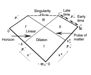
Figure 1: Penrose diagram for CGHS spacetime.

At $x^{+}<x^{+}_{0}$, the metric is Minkowskian, usually known as the dilaton vacuum (region I and I’), given by ${ds^{2}=-\frac{dx^{+}dx^{-}}{-\Lambda^{2}x^{+}x^{-}},}$ whereas, at $x^{+}>x^{+}_{0}$ it is represented by the black hole metric (region II, III) $ds^{2}=-\frac{dx^{+}dx^{-}}{\frac{M}{\Lambda}-\Lambda^{2}x^{+}(x^{-}+\Delta)}.$ These (null) Kruskal coordinates ($x^{+},x^{-}$) are useful in presenting the global structure of the spacetime. On the other hand, for physical studies involving Quantum Field Theory (QFT) in curved space-time, it is often convenient to use coordinates associated with physically interesting observers in various regions. In the dilation vacuum region, natural Minkowskian coordinates are $y^{+}=\frac{1}{\Lambda}\ln(\Lambda x^{+}),y^{-}=\frac{1}{\Lambda}\ln(-{\frac{x^{-}}{\Delta}})$, and the metric is expressed as $ds^{2}=-dy^{+}dy^{-}$ with $-\infty<y^{-}<\infty;~{}-\infty<y^{+}<\frac{1}{\Lambda}\ln(\Lambda x_{0}^{+})$. On the other hand, on the BH exterior (region II), where the long lived physical observers might exist, one has the coordinates $\sigma^{+}=\frac{1}{\Lambda}\ln(\Lambda x^{+})=y^{+},\sigma^{-}=-\frac{1}{\Lambda}\ln(-\Lambda(x^{-}+\Delta))$, so that the metric is $ds^{2}=-\frac{d\sigma^{+}d\sigma^{-}}{1+(M/\Lambda)e^{\Lambda(\sigma^{-}-\sigma^{+)}}}$ with $-\infty<\sigma^{-}<\infty$ and $\sigma^{+}>\sigma_{0}^{+}=\frac{1}{\Lambda}\ln(\Lambda x_{0}^{+}).$ We can see the asymptotic flatness by expressing this metric in Schwarzschild like coordinates ($t,r$) defined by $\sigma^{\pm}=t\pm\frac{1}{2\Lambda}\ln(e^{2\Lambda r}-M/\Lambda)$ so that, we have ${ds^{2}=-(1-\frac{M}{\Lambda}e^{-2\lambda r})dt^{2}+\frac{dr^{2}}{(1-\frac{M}{\Lambda}e^{-2\lambda r})}}$. The Kruskal coordinates $2T=x^{+}+x^{-}+\Delta,~{}2X=x^{+}-x^{-}-\Delta$ can be related with Schwarzschild like time $t$ and space $r$ coordinates using $\tanh(\Lambda t)=T/X$ and $-\frac{1}{\Lambda^{2}}(e^{2\Lambda r}-M/\Lambda)=T^{2}-X^{2}$.

Next, we consider the quantum description of the field $f$ for which one uses ${\mathscr{I}}^{-}_{L}\cup{\mathscr{I}}^{-}_{R}$ as the asymptotic past (in) region, and the black hole (exterior and interior) region as the asymptotic out region. The in description of the quantum field operator can be expanded as $\hat{f}(x)=\sum(\hat{f}_{\omega}^{R}(x)+\hat{f}_{\omega}^{L}(x)),$ where $f_{\omega}^{R/L}=\hat{a}_{\omega}^{R/L}u_{\omega}^{R/L}+\hat{a}^{R/L{\dagger}}_{\omega}u_{\omega}^{R*/L*}$. Here, the basis of functions (modes) are: ${u_{\omega}^{R}=\frac{1}{\sqrt{2\omega}}e^{-i\omega y^{-}}}$ and ${u_{\omega}^{L}=\frac{1}{\sqrt{2\omega}}e^{-i\omega y^{+}}},$ with $\omega>0$. The superscripts $R$ and $L$ mean right and left moving modes. These modes thus specify a right in vacuum ($\left|0_{in}\right\rangle_{R}$), and a left in vacuum ($\left|0_{in}\right\rangle_{L}$), whose tensor product ($\left|0_{in}\right\rangle_{R}\otimes\left|0_{in}\right\rangle_{L}$) defines our in vacuum. One can also expand the field in the out region in terms of the complete set of modes that (at late times) have support in the outside (exterior) and inside (interior) of the event horizon, respectively. Therefore the field operator has the form $\hat{f}(x)=\hat{f}_{out}^{R}(x)+\hat{f}_{out}^{L}(x)$ where,

$$\hat{f}_{out}^{R/L}(x) = \sum_{\omega}\hat{b}_{\omega}^{R/L}v_{\omega}^{R/L}+\qquad\hat{b}^{R/L{\dagger}}_{\omega}v_{\omega}^{R*/L*}$$ (3)

$$+\sum_{\tilde{\omega}}\hat{b}_{\tilde{\omega}}^{R/L}v_{\tilde{\omega}}^{R/L}+\hat{b}^{R/L{\dagger}}_{\tilde{\omega}}v_{\tilde{\omega}}^{R*/L*},$$

where we use the convention in which modes with and without tildes are associated with having support inside and outside the horizon, respectively. The corresponding operators are similarly labeled. We note that , as will be further argued in the last section, the arbitrariness in the choice of modes inside the horizon will not affect our physical results. The mode functions in the exterior to the horizon that we will use are: ${v_{\omega}^{R}=\frac{1}{\sqrt{2\omega}}e^{-i\omega\sigma^{-}}\Theta(-(x^{-}+\Delta))}$ and ${v_{\omega}^{L}=\frac{1}{\sqrt{2\omega}}e^{-i\omega\sigma^{+}}\Theta(x^{+}-x_{0}^{+}).}$ Similarly, one can define a set of modes in the black hole interior so that the basis of modes in the out region is complete. For the left moving modes, we maintain the same choice as before, while for the right moving mode, we use ${\hat{v}_{\tilde{\omega}}^{R}=\frac{1}{\sqrt{2\tilde{\omega}}}e^{i\tilde{\omega}\sigma_{in}^{-}}\Theta(x^{-}+\Delta)}$. Following cghs-more , we replace the above delocalized plane wave modes by a complete orthonormal set of discrete wave packets modes, $v_{nj}^{L/R}=\frac{1}{\sqrt{\epsilon}}\int_{j\epsilon}^{(j+1)\epsilon}d\omega e^{2\pi i\omega n/\epsilon}v_{\omega}^{L/R},$where the integers $j\geq 0$ and $-\infty<n<\infty$. These wave packets are peaked about $\sigma^{+/-}=2\pi n/\epsilon$ with width $2\pi/\epsilon$ respectively.

The non-trivial Bogolubov transformations are only relevant in the right moving sector, and the corresponding transformation from in to exterior modes is what accounts for the Hawking radiation. As is well known, the fact that the initial state, corresponding to the vacuum for the right moving modes, and the left moving pulse forming the black hole $\left|\Psi_{in}\right\rangle=\left|0_{in}\right\rangle_{R}\otimes\left|Pulse\right\rangle_{L}$ can be written as:

$$N\displaystyle\sum_{F_{nj}}C_{F_{nj}}\left|F_{nj}\right\rangle^{ext}\otimes\left|F_{nj}\right\rangle^{int}\otimes\left|Pulse\right\rangle_{L},$$ (4)

where the states $\left|F_{nj}\right\rangle$ are characterized by the finite occupation numbers $\{F_{nj}\}$ for each corresponding mode $n,j$, $N$ is a normalization constant, and the coefficients $C_{F_{nj}}$’s are determined by the Bogolubov transformations. If one now decides to ignore the degrees of freedom (DOF) of the quantum field lying in the black hole interior, and to describe just the exterior DOF, one passes, as usual, to a density matrix description. Thus, we would obtain the reduced density matrix by tracing over the interior DOF, and we end up, as is well known, with a density matrix corresponding to a thermal state. Note that this density matrix represents in the language of dEspagnat ; timpson , an improper mixture as it arises from ignoring part of the system, which as a whole is in a pure state. We will thus say that what we have at this point is an improper thermal state. As we said before, in this paper we will obtain a proper thermal state.

III.2 CSL evolution of quantum fields in CGHS background

We are now in a position to show how a thermal state, corresponding to a proper mixture, is obtained using our adapted version of CSL, and some reasonable assumptions about QG. As the CSL theory involves a modification of the time evolution of the quantum states, we need a foliation of our space-time associated with a “global time parameter”. As is customary in QFT, we will be using an interaction-type picture, where the free part of the evolution is encoded in the field operators, and the interaction, which in our case is just the new CSL part, drives the evolution of the states. In a relativistic context, based in a truly covariant version of CSL, one would be using a Tomonaga-Schwinger type of evolution equation.

Let us now briefly comment on the application of CSL to the CGHS model. In order to describe the CSL evolution we first need to foliate the spacetime with Cauchy slices which are defined in the following manner. We choose a $r=const.$ and a $t=const.$ surfaces in the inside and outside of the horizon, respectively, and then join them using a surface $T=const$ (see Figure (2)). We specify the juncture points (i.e., the points of intersection between $r=const.$ with $T=const.$ inside the horizon as well as $T=const.$ and $t=const$ outside the horizon) by two curves, $T_{1,2}(X)$. We take $T_{1}(X)=\left(X^{2}+\frac{M}{\Lambda^{3}}e^{-2\Lambda/\sqrt{X}}\right)^{1/2}$ and $T_{2}(X)$ is found by reflection of $T_{1}(X)$ with respect to the horizon $T=X$. Note that this choice for the intersection curves is not unique and many other choices are acceptable. However it is essential that the slices be Cauchy hypersurfaces.

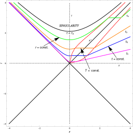
Figure 2: Spacetime foliation plots for the CGHS spacetime.

With this construction, we can now introduce a “global time parameter” $\tau$ specifying the hyper surfaces of the foliation by the value of its intersect with the $T$ axis. This foliation covers the complete “BH region” (exterior and interior) and one can extend it to past vacuum region arbitrarily with no effect in our study, simply because, the CSL modification in the dynamics is significant only inside the black hole (more precisely, close to the singularity).

Now, we must select the operators driving the collapse in our version of CSL evolution. We note, as was already mentioned, that the CSL equations can be generalized to drive the collapse process leading to one element of the joint eigen- basis of the set of commuting operators $\{A^{\alpha}\}$ which we call the collapse operators. For each $A^{\alpha}$ there is one stochastic function $w^{\alpha}(t)$, and the evolution equation takes the form:

$${|\psi,t\rangle_{w}=\hat{\cal T}e^{-\int_{0}^{t}dt^{\prime}\big{[}i\hat{H}+\frac{1}{4\lambda}\sum_{\alpha}[w^{\alpha}(t^{\prime})-2\lambda\hat{A}^{\alpha}]^{2}\big{]}}|\psi,0\rangle.}$$ (5)

In standard non-relativistic CSL on flat spacetime, and as previously noted, one takes these to be the (smeared) position operators so that the collapse takes place in ”position space” so as to literally localize the wave function. In the situation at hand we will use, for simplicity, the particle number operators (see footnote 3), so that, given that $\lambda$ becomes large only in regions of high space-time curvature the states will collapse to a state with definite number of particles in the inside region. Far from the singularity the rate of collapse will be much smaller, and the direct effects of CSL evolution will be almost negligible (i.e. just as the ones of the original version of CSL).

We should note here that, we have selected these collapse driving operators for simplicity of the calculations but other choices can be expected to yield essentially the same end result. The basic reason for that is that the relevant collapse operators will be associated with the regions near the curvature singularity which lies inside the horizon, and the fact that CSL theory is known not to lead to faster than light communication in EPR-B type situations NLcollpase . We can understand this by recalling that even in simplistic versions of theories involving measurement-related collapse, such as the Copenhagen interpretation of quantum mechanics, for an EPR-B situation, the choices made by Bob on what observable to measure in his part of the entangled pair, can not be used to send a signal to Alice, who will, for all the possible choices made by Bob, observe the same statistical results in all her possible observations. As we know, it is only by measuring correlations between the two sides, that something nontrivial can be said in such cases. In other words, the observers outside will find the same statistical distribution of results for all possible observations regardless of what “nature measures” (by this we mean “in what basis, does the fundamental CSL type theory actually collapse our quantum field states”) in the black hole interior.

As we have mentioned before, our version of CSL in curved space-time is taken to have a curvature dependent $\lambda$. Concretely, we will assume here that $\lambda$ depends, in this 2-dimensional situation, on the Ricci scalar $R$ according to:

$${\lambda(R)=\lambda_{0}\left[1+\left(\frac{R}{\mu}\right)^{\gamma}\right]}$$ (6)

where $\gamma\geq 1$ is a constant, $\mu$ provides an appropriate scale and $\lambda_{0}$ is the standard CSL rate of collapse comment . It should be noted that, in a more realistic 4-dimensional model one should have a $\lambda$ depending on Weyl scalar ($W_{abcd}W^{abcd}$) as mentioned in Okon:2013lsa .

Note that the hypersurfaces given by our chosen foliation in Figure (2) have constant $R$ inside the black hole (in almost all the part of $\Sigma_{\tau}$ that lies inside) and the value of $R$ is increasing towards the singularity. As a result, Cauchy slices with larger $\tau$ have, inside the horizon, a larger value of $\lambda$ (inside the horizon we have $R=\frac{4M\Lambda}{M/\Lambda-(T^{2}-X^{2})}=\frac{4M\Lambda}{M/\Lambda-\Lambda^{2}\tau^{2}}$). Therefore, although the CSL evolution allows us to evolve the state of the quantum field from one Cauchy slice to another, the effective collapse will take place only in the interior part of the slicing, while its effect on the exterior portion will not be significant. Of course, there will be an indirect effect to the quantum field states defined with respect to the exterior Fock space, since these states are entangled with the internal field states. When the collapse takes place for the inside DOF, to the eigenstate of number operator defined inside, it will automatically collapse also the exterior quantum states to a definite particle number, but that, of course, does not affect the statistical results obtained by the outside observers as explained before.

Thus, for the region of interest we have $\lambda=\lambda(\tau)$ and the resulting evolution will achieve in the finite “time” to the singularity (i.e., $\tau=\tau_{s}=\frac{M^{1/2}}{\Lambda^{3/2}}$), what ordinary CSL achieves in an infinite amount of time. In this time the CSL evolution will drive the state to one of the eigenstates of the collapse operators. Recall that the particle content of state $\left|F\right\rangle$ is given by the particle distribution $F=\{\dots,F_{nj},\dots\}$ where $F_{nj}$ is the number of particles in mode $v_{nj}$ (both for the inside of the black hole and the outside). It should be noted that the collapse process avoids generating singularities in the energy-momentum tensor when we take smeared versions of these number operators. That ensures that no “firewall” type situations would arise far from the singularity. The action of the number operator $N^{int}_{nj}$ acting on $\mathscr{F}^{int}$ is ${\hat{N}^{int}_{nj}\left|F\right\rangle^{int}=F_{nj}\left|F\right\rangle^{int}}.$ The set of collapse operators we are contemplating are:

$${\hat{A^{\alpha}}=\hat{N^{int}_{nj}}\otimes\mathbb{I}^{ext}}$$ (7)

for all $n,j$, where $\mathbb{I}^{ext}$ is the identity operator in $\mathscr{F}^{ext}$. Thus the quantum states corresponding to interior Fock space will tend to collapse to the joint eigenstates of $\hat{N^{int}_{nj}}$ with definite particle content, whereas states in the exterior Fock space will remain essentially unaffected by the collapse dynamics. As we said, the only significant effect on external states will be that due to the entanglement with internal quantum states of the black hole.

With the above construction we are now in a position to show how quantum evolution takes place in our model. We will do that, first, for a single system (which is given in (4)), and later, for an ensemble of systems prepared in the same initial state.

Let us consider the first case. The fact that CSL evolves states towards one of the eigenstates of the collapse operators (7) ensures that, as the result of the evolution (5), the state at a hypersurfaces $\tau=const.$, that comes very close to the singularity (on $\Sigma_{\tau_{s}-\epsilon}$ in Fig. 3), would be of the form:

$${\left|\Psi_{in,\tau}\right\rangle=N\displaystyle C_{F_{nj}}\left|F_{nj}\right\rangle^{ext}\otimes\left|F_{nj}\right\rangle^{int}\otimes\left|Pulse\right\rangle_{L}}.$$ (8)

Note that there is no summation, so the state is pure, even though it is undetermined, simply because we don’t know the actual realization of the stochastic functions $w_{nj}$.

Note that, although individual states with definite occupation number in the ext and int modes such as the one above lead to singular $\langle T_{ab}\rangle$, those states are only approached asymptotically as $\tau\to\tau_{s}$. The dynamics of CSL generates only smooth states prior to the singularity ARXIVE . The situation is analogous to the measurement of a precise number of Rindler particles in the Minkowski vacuum in a finite time, which is impossible unless the field-detector interaction is singular wald-pc .

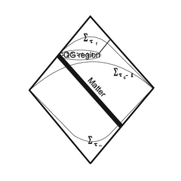
Figure 3: Plausible space-time structure including the post-singularity region.

IV Role of quantum gravity and the final result

We have characterized the state after the CSL evolution (8) defined on a Cauchy slice that comes very close to the singularity, and thus we must now consider the role of quantum gravity, to pass to the final hypersurface $\Sigma_{\tau_{f}}$ in Fig. 3. For that, we shall make some seemingly natural assumptions about QG. We will assume that a reasonable theory of QG will resolve the singularity and lead, on the other side, to a reasonable space-time. Moreover, we will assume that such a theory will not lead to large violations of the basic space-time conservation laws. With these assumptions, we now look at the situation on the region just before the singularity: There, from the energetic point of view, we have the following: i) The incoming positive energy flux corresponding to the left moving pulse that formed the BH. ii) The incoming flux (from region II to region III in Fig. 1) of the left moving vacuum state for the rest of the modes which is known to be negative and essentially equal to the total Hawking Radiation flux. iii) The flux associated with the right moving modes that crossed the collapsing matter (from region I’ to III) but fell directly into the singularity.

The only energy missing in the budget above is that associated with the Hawking radiation flux. If energy is to be essentially conserved by QG, it seems that the only possibility for the state in the “post singularity region” is one corresponding to a very small value of the energy. Such state of negligible energy might be associated with some remnant radiation, or perhaps a compact and stable remnant with something close to Planck’s mass. Those possibilities would represent a case were a small amount of information survives the whole process, and will be ignored hereafter for simplicity. Instead, we will consider the simplest alternative: A zero energy momentum state corresponding to a “trivial” region of space-time. We denote it by $\left|0^{p.s.}\right\rangle$ (post-singularity). In other words, we complete our characterization of the evolution, by assuming that the effects of QG can be represented by the curing of the singularity, and by the transformation:

$${\left|\Psi_{in,\tau}\right\rangle=N\displaystyle C_{F_{nj}}\left|F_{nj}\right\rangle^{ext}\otimes\left|F_{nj}\right\rangle^{int}\otimes\left|Pulse\right\rangle_{L}}$$

$${\to N\displaystyle C_{F_{nj}}\left|F_{nj}\right\rangle^{ext}\otimes\left|0^{p.s.}\right\rangle}.$$

The above result might seem a bit unsettling, because we end up with a pure quantum state, while, if information is lost in the full process, we should end with a mixed (thermal) density matrix. The point, of course, is that the theory does not predict which one of the possible pure states we will end up with. That depends on the particular realization of the random functions $w^{\alpha}$ that appears in the CSL evolution equation.

Thus, as a consequence of the inherent stochasticity of the theory, all we can do is to make statistical predictions. In fact, we can easily do that by considering the case where an ensemble of systems are identically prepared in the same initial state:

$${\left|\Psi_{in}\right\rangle=\left|0_{in}\right\rangle_{R}\otimes\left|Pulse\right\rangle_{L}}.$$

We then describe this ensemble by the pure density matrix ${\rho(\tau_{0})=\left|\Psi_{in}\right\rangle\left\langle\Psi_{in}\right|}$. In each case the pulse will lead to the formation of a black hole. As before, CSL evolution is the dominant where the curvature becomes large, i.e., before reaching the singularity, or more precisely the quantum gravity regime (i.e. the hypersurface $\Sigma_{\tau_{s}-\epsilon}$). The evolution from initial hypersurface $\Sigma_{\tau_{0}}$ to an intermediate hypersurface $\Sigma_{\tau}$ is then given by

$${\rho(\tau)={\cal T}e^{-\int_{\tau_{0}}^{\tau}d\tau^{\prime}\frac{\lambda(\tau^{\prime})}{2}\sum_{nj}[\tilde{N}_{nj}^{L}-\tilde{N}_{nj}^{R}]^{2}}\rho(\tau_{0})}.$$ (9)

We express $\rho(\tau_{0})=\left|0\right\rangle^{in}\left\langle 0\right|^{in}$ in terms of the out quantization (ignoring left moving modes as they are not relevant for the external observers):

$${\rho(\tau_{0})=N^{2}\sum_{F,G}e^{-\frac{\pi}{\Lambda}(E_{F}+E_{G})}\left|F\right\rangle^{int}\otimes\left|F\right\rangle^{ext}\left\langle G\right|^{int}\otimes\left\langle G\right|^{ext}},$$

where $\Lambda$ is the parameter of the CGHS model and $E_{F}\equiv\sum_{nj}\omega_{nj}F_{nj}$ is the energy of the state $\left|F\right\rangle^{ext}$ with respect to late-time observers near $\mathscr{I_{R}}^{+}$.

The operators $\tilde{N}_{nj}$ and their eigenvalues are independent of $\tau$. Thus we have,

$$\rho(\tau)=N^{2}\sum_{F,G}e^{-\frac{\pi}{\Lambda}(E_{F}+E_{G})}{\cal B}{\left|F\right\rangle^{int}\otimes\left|F\right\rangle^{ext}\left\langle G\right|^{int}\otimes\left\langle G\right|^{ext}},$$

where ${\cal B}\equiv e^{-\sum_{nj}(F_{nj}-G_{nj})^{2}\int_{\tau_{0}}^{\tau}d\tau^{\prime}\frac{\lambda(\tau^{\prime})}{2}}$. In general, this equation does not represent a thermal state. Nevertheless, as $\tau$ approaches the singularity, say at $\tau=\tau_{s}$, the integral $\int_{\tau_{0}}^{\tau}d\tau^{\prime}\lambda(\tau^{\prime})/2$ diverges since $\lambda(\tau)$ becomes large on hypersurfaces of high curvature (as we have assumed $\gamma\geq 1$ in (6)). Then, as $\tau\to\tau_{s}$ the non diagonal elements of $\rho(\tau)$ cancel out and we have:

$${\lim_{\tau\to\tau_{s}}\rho(\tau)=N^{2}\sum_{F}e^{-\frac{2\pi}{\Lambda}E_{F}}\left|F\right\rangle^{int}\otimes\left|F\right\rangle^{ext}\left\langle F\right|^{int}\otimes\left\langle F\right|^{ext}}.$$

If we now include the left moving pulse, and take into account what we have assumed about the role of QG, we obtain a density matrix characterizing the ensemble after the singularity (on $\Sigma_{\tau_{f}}$ in Fig. 3), which is given by

$$\rho^{Final} = N^{2}\sum_{F}e^{-\frac{2\pi}{\Lambda}E_{F}}\left|F\right\rangle^{ext}\otimes\left|0^{p.s.}\right\rangle\left\langle F\right|^{ext}\otimes\left\langle 0^{p.s.}\right|.$$ (10)

$$\equiv\left|0^{p.s.}\right\rangle\left\langle 0^{p.s.}\right|\otimes\rho^{ext}_{Thermal}$$

That is, we started with an ensemble described by a pure state of the quantum field corresponding to the vacuum plus an initially collapsing pulse, and the corresponding space-time initial data on past null infinity, and ended up, with a proper thermal state. In other words, we ended up with a proper mixture (recall the terminology from dEspagnat ; timpson ), characterizing an ensemble of systems with a thermal distribution on future null infinity followed by an empty region.

V Summary and discussions

We have studied, at the quantitative level, a concrete realization of the idea that a resolution of the black hole information conundrum might be related to the solution of the measurement problem in quantum mechanics. We have seen how a proposal developed for addressing the latter can be adapted to the black hole setting, and that by assuming that the parameter controlling the departure from the usual quantum mechanical unitary evolution increases with space-time curvature, we are led to a picture whereby the information loss, one can naively infer as occurring in the latter case, becomes a direct and actual result of the modified dynamics. This leads to a situation where the information loss associated with the full evaporation of a black hole via Hawking radiation can be seen, not as a paradoxical result, but as the natural outcome from the fundamental quantum evolution that accounts for the physics of both micro and macro objects.

Of course, we assumed that a QG theory would resolve the singularity, and otherwise be reasonable so that it does not lead to gross violations of conservation laws, with potentially observable implications in the regions where something close to a classical space-time description is expected.

We should also acknowledge that in the course of this work we made several simplifying assumptions, and ignored some issues that are not easy to deal with, but we think that there are good reasons to expect that the general picture we obtained is rather robust. We next deal briefly with the most important of these approximations and issues:

1. Choice of collapse operators: The general choice of the operators $A_{\alpha}$ controlling the CSL dynamics is clearly an open issue. As we already mentioned, a complete theory should specify, for all possible circumstances, and in a manner that depends only on the dynamics of the system in question, what determines such operators. It seems that they must correspond to a kind of smeared position operators, in the case where the system can be described in terms of the non-relativistic quantum mechanics of many particles. The choice of the particle number operator in the interior of black hole region that we made in section III.2, was clearly done for convenience. In a fully covariant theory we expect these operators to be locally constructed from quantum fields, and the number operators are clearly non-local. It should be pointed out, however, that in these theories, one can rewrite the same CSL evolution in terms of various and very different choices of operators, as is in fact shown explicitly in the work pedro . On the other hand, as we already noted in connection with EPR-B situations, the collapse of the state into eigenvalues of an operator associated with a certain space-time region has no influence whatsoever, in the effective description, in terms of a density matrix, for the state restricted to space-time regions that are causally disconnected. Of course, in the case of an EPR experiment, one could still consider the correlations between the outcomes of Alice vs. Bob measurements, and those will clearly depend on what quantity did each one measure. However, in our case, the state of the subsystem corresponding to Bob (i.e. the matter field in the inside BH Region) will simply disappear. That is, in the post Quantum Gravity region the state will correspond to a sort of vacuum state containing almost no energy or information, so that there would be (almost) no other correlations to look for. We fully expect such robustness (i.e., independence of the precise choice of collapse operators in the region III) to apply to the characterization of the state of the field in $\mathscr{I}^{+}_{R}$ in terms of a density matrix.

2. Relativistic Covariance: The model we have employed is based on a non-relativistic spontaneous collapse theory, and it is clear that a satisfactory proposal to deal with the issue at hand should be based on a fully covariant theory. We should note, in this regard, the early studies advances , and the recent specific proposals for special relativistic versions of these type of theoriesTumulka-Rel ; Bedingam-Rel ; RelColPearle . In those theories the evolution, in the interaction picture approach we have been using, should be describable in terms of a Tomonaga-Schwinger evolution equation where, instead of the interaction hamiltonian, we would have the corresponding collapse theory density operator. We hope eventually to adapt the present scenario to those proposals, a task we expect to be rather nontrivial.

3. Choice of foliation: We have presented the analysis using a very particular foliation. Within a covariant setting, we can expect that any specific physical prediction should be independent of the foliation. One important consequence would be that, whenever we consider a foliation passing through a region of space-time which is far from the singularity, the changes in the state around that point, associated with the CSL type modifications, should have effects in local operators that will be very small, simply because the CSL-like parameter $\lambda$ will be small there. This indicates that we should not encounter anything like “firewalls” in the region of the horizon which is far from the singularity.

4. Energy conservation: One might be concerned that, when considering an individual situation, the energy of the initial pulse of matter might not be exactly equal to that corresponding to the state with definite number of particles $\left|F\right\rangle^{ext}_{R}$ that characterizes the modified matter content in the asymptotic region, once the black hole has evaporated completely. The first thing to note is that CSL, in general, leads to small violations of energy conservation and that issue, in fact, has led to the establishment the most stringent bounds on the parameter $\lambda$ (although modified covariant theories might evade this problems altogether. See for instance the detailed discussions in Bedingam-Rel ; Unruh-Wald ). The second thing to note is that if there is small amount of energy remaining inside the black hole region, and very close to the singularity, simply because the positive and negative energy fluxes do not cancel each other exactly, there would seem to be no problem, at least in principle, if such energy is radiated after the singularity. In that way, most of the initial energy will be radiated in the standard Hawking radiation, and a very small amount of energy, carrying a minuscule amount of information, would remain to be radiated towards infinity from the “quantum gravity region”.

5. Back reaction: We must note that, in all the discussion so far, we have omitted the very important issue of back reaction. The changes in the space-time metric as a response to those in state of the matter fields, are essential, if we want to account for the decrease of the mass of the black hole as a result of the Hawking radiation taking energy to infinity. That, in turn, is an essential aspect of the arguments involving overall energy conservation. Going further, the change in the space-time metric, and, in particular, in the black hole’s mass, and its “instantaneous Hawking temperature” in a more realistic model, are expected to modify the nature of the radiation, so that, the “late time” radiation would be, in a sense, emitted at a higher temperature than the “early times” one, leading to the runaway effects that are associated with the expectation of an explosive disappearance of the black hole itself. It is clear that all such effects are extremely important in obtaining a realistic picture of the entire history of formation and complete evaporation of a black hole. However, there seems to be no reason to expect that those important changes will modify, in an essential way, the workings of the proposal we have been considering here. In fact, the back reaction is essential, in accounting for the decrease of the Bondi mass to a very small value, as one considers the very late parts of $\mathscr{I}^{+}_{R}$. This, in turn, is what allows us to consider, matching the asymptotic region with the space-time that is expected to emerge on the other side of the quantum gravity region that replaces the “would be singularity”, and which, as we have indicated, should be thought as essentially empty and flat, (with the caveats discussed in the item above).

On the other hand, it seems that theories involving spontaneous reduction of the quantum state of matter fields should facilitate, at least at the conceptual level, the treatment of back reaction, simply because there is a clear state that should be used in evaluating the expectation value of the energy momentum tensor at each hypersurface: in our case the state associated to that hyperurface by the CSL dynamics. Of course, as indicated before, a fully satisfactory account would have to rely on a fully covariant theory corresponding to general relativistic generalizations of those recently proposed inTumulka-Rel ; Bedingam-Rel ; RelColPearle , and, as discussed in those works, the appropriate state to be used in computing the expectation value of an operator associated with a given space-time “event” $p$, would be the state associated with the past null cone of $p$ (more precisely one would need to consider open regions around $p$ and the state associated with the boundary of the causal past of those). Nevertheless, and despite the discussion below, it is clear that the technical aspects of the treatment of back reaction need to be further analyzed and developed (particularly in view of the footnote 10 below, and related comments) if one wants to have a viable, even if only approximate, semi-classical account of the black hole evaporation process.

6. Reliance on semi-classical gravity: The previous item forces us to consider the basic viability of semi-classical gravity, the scheme where one treats the space-time metric at the classical level, but uses as a source in Einstein’s equation the quantum expectation value of the energy momentum tensor. This question has been considered in a well known paper by Page and Geilker Page . That work is often referred to, as indicating that semi-classical gravity is simply at odds with experimental results. However, what is not often noted is that such conclusion is only valid in the contexts where quantum mechanical evolution does not include any sort of measurement-related or spontaneous collapse. Thus it certainly would not be relevant for our proposal. On the other hand, it is clear that if one wants to incorporate the reduction or the collapse of the quantum state of matter fields, the semi-classical equation, taken to be fundamental and 100% accurate, would not be viable, as it is simply inconsistent. The point however is that if one takes the metric description of space-time as merely an effective and approximate characterization, in analogy, say, with Navier -Stokes (NS) equation in hydrodynamics, one would not expect the equation to hold exactly, or to be valid universally. That is, just as there would be situations where the NS would not be an appropriate characterization of the fluid, such as when an ocean wave breaks, and in which one can expect important local departures from the equation, one can expect something analogous to occur with the semi-classical Einstein equation. This, however, would not invalidate the equation in its use for some suitable macroscopic and approximate characterizations. More precise characterizations, both in the treatment of fluids and of gravitation, can be expected to involve higher order and more complicated terms, and, of course eventually, as the natural scale of the more fundamental and underlying theory is approached, one would expect the complete breakdown of the effective description. Some initial steps in the exploration of the formal adaptation of this approach to the use of semi-classical gravity in a cosmological context have been considered in Alberto . We should also note the work Carlip in which the general arguments against semi-classical gravity were critically considered, concluding that they are not as robust as it might have seemed initially.

Finally, it is worth mentioning a rather speculative, but very suggestive point made in Okon-New . The general picture that one obtains in this way of dealing with the BH information question has the kind of intrinsic self consistency of a boot-strap model: if black hole evaporation is associated with loss of information and departure from quantum unitarity, then, it is natural, to consider that virtual, microscopic black holes, generated ”off-shell” in radiative quantum processesGeorge , should themselves lead to loss of information and departure of unitarity in all situations, and that could, perhaps, be the source of the effects which one parametrizes, at the effective level, as the modifications of quantum mechanics represented in CSL and related theories. The tail-baiting snake picture, would then, be complete.

We reiterate that, at this point, this work represents just a toy model, as, in particular, all items above would need to be addressed in any realistic version. However, we believe that reasonable models with the basic features we have discussed here do offer a rather interesting path to resolving the long standing conundrum known as the “Black Hole Information Loss Paradox” and, to do so in connection with the attempts to resolve, what we, and various other colleagues, but certainly not the majority, regard as a very unsettling aspect of our current understanding of quantum theory: the “measurement problem”.

Acknowledgment: We thank Robert Wald, Philip Pearle and Elias Okon for discussions. DS is supported by the CONACYT-México Grant No. 220738 and UNAM-PAPIIT Grant No. IN107412. SKM and LO are supported by DGAPA fellowships from UNAM.

References

- (1) S. W. Hawking, Phys. Rev. D 14, 2460 (1976).
- (2) R. M. Wald, Quantum Field Theory in Curved Spacetime and Black Hole Thermodynamics (The University of Chicago Press, 1994).
- (3) E. Okon and D. Sudarsky. Found. Phys. 45, Issue 4, 461-470 (2015) [arXiv: 1406.2011 [gr-qc]].
- (4) J. M. Maldacena, JHEP 0304, 021 (2003).
- (5) A. Ashtekar, V. Taveras and M. Varadarajan, Phys. Rev. Lett. 100, 211302 (2008).
- (6) S. D. Mathur, Journal of Physics: Conference Series 462 (2013) 012034.
- (7) M. Bojowald [arXiv:1409.3157 [gr-qc]].
- (8) A. Almheiri, D. Marolf, J. Polchinski and J. Sully, JHEP 1302, 062 (2013).
- (9) S. W. Hawking [arXiv:1401.5761 [hep-th]]; B. D. Chowdhury and L. M. Krauss [arXiv:1409.0187 [gr-qc]].
- (10) J. Maldacena and L. Susskind, Fortsch. Phys. 61, 781 (2013) [arXiv:1306.0533 [hep-th]].
- (11) R. Penrose, The Emperor’s New Mind (Oxford University Press, 1989)); in Physics meets philosophy at the Planck scale, edited by C. Callender (Cambridge University Press, 2001).
- (12) R. Penrose, in Quantum Gravity II, edited by C. J. Isham, R. Penrose and D. W. Sciama (Clarendon Press, Oxford, 1981).
- (13) E. Wigner, Am. J. of Physics 31, 6 (1963); A. Lagget, Prog. Theor. Phys. Suppl. 69, 80 (1980); J. Bell, in Quantum Gravity II, edited by C. J. Isham, R. Penrose and D. W. Sciama (Clarendon Press, Oxford, 1981); D. Albert, Quantum Mechanics and Experience (Harvard University Press, 1992), Chap. 4 and 5; D. Home, Conceptual Foundations of Quantum Physics: an overview from modern perspectives (Plenum, 1997), Chap. 2.
- (14) For reviews: M. Jammer, Philosophy of quantum mechanics. The interpretations of quantum mechanics in historical perspective (John Wiley and Sons, New York, 1974); R. Omnes, The Interpretation of Quantum Mechanics (Princeton University Press 1994); and the more specific critique: S. L. Adler, Stud. Hist. Philos. Mod. Phys. 34, 135-142 (2003).
- (15) J. S. Bell, (Cambridge University Press, 1987); Phys.World 3, 33 (1990).
- (16) T. Maudlin, Topoi 14(1), 715 (1995).
- (17) D. Bohm and J. Bub, Rev. Mod. Phys. 38, 453 (1966).
- (18) P. Pearle, Phys. Rev. D 13, 857 (1976); Int. J. Theor. Phys. 18, 489 (1979).
- (19) G. Ghirardi, A. Rimini and T. Weber, in Quantum Probability and Applications, edited by A. L. Accardi (Springer, Heidelberg,1985), pages 223-232; Phys.Rev. D 34, 470 (1986).
- (20) P. Pearle, Phys. Rev. A 39, 2277 (1989).
- (21) G. Ghirardi, P. Pearle and A. Rimini, Phys. Rev. A 42, 7889 (1990).
- (22) L. Diosi, Phys. Lett. A 105, 4 (1984), p. 199-202; Phys. Lett. A 120, 377 (1987) ; Phys. Rev. A 40, 1165 (1989).
- (23) S. Weinberg, Phys. Rev. A 85, 062116 (2012) [arXiv:1109.6462 [quant-ph]].
- (24) W. G. Unruh and R. M. Wald, Phys. Rev. D 52, 2176 (1995).
- (25) B. d’Espagnat, Conceptual Foundations of Quantum Mechanics (Addison Wesley, 2nd. edition, 1976).
- (26) C.G. Timpson and H.R. Brown, Int. J. Quantum Inf. 3(4), 679 (2005).
- (27) C. G. Callan, S. B. Giddings, J. A. Harvey, and A. Strominger, Phys. Rev. D 45, R1005 (1992).
- (28) For a recent review see for instance: A. Bassi, K. Lochan, S. Satin, T. P. Singh and H. Ulbricht, Rev. Mod. Phys. 85, 471 (2013) [arXiv:1204.4325 [quant-ph]].
- (29) J. Martin, V. Vennin and P. Peter [arXiv:1207.2086]; S. Das, K. Lochan, S. Sahu, and T.P. Singh, Phys. Rev. D, 88(8), 085020 (2013) [arXiv:1304.5094 [astro-ph.CO]].
- (30) P. Cañate, P. Pearl and D. Sudarsky, Phys. Rev. D, 87, 104024 (2013) [arXiv:1211.3463[gr-qc]].
- (31) For a more detailed discussion and motivation of this issue see: S. K. Modak, L. Ortíz, I. Peña and D. Sudarsky [arXiv:1406.4898].
- (32) S. B. Giddings and W. M. Nelson, Phys. Rev. D 46, 2486 (1992); A. Fabbri and J. Navarro-Salas, Modeling Black Hole Evaporation (Imperial College Press, London, 2005).
- (33) See for instance the discussions in: D. J. Bedingham, [arXiv:0907.2327 [quant-ph]], and also in G. C. Ghirardi, Foundations of Physics Letters 9, 313 (1996); G. C. Ghirardi, A. Rimini and T. Weber, Letter Al Nuovo Cimento 27, 293 (1980); G. C. Ghirardi, R. Grassi, J. Butterfield and G. N. Fleming, Foundations of Physics, 23, 341 (1993); G. C. Ghirardi and R. Grassi, Studies in History and Philosophy of Modern Physics 25, 397 (1994).
- (34) The original CSL theory was developed as a modification of non-relativistic many particle quantum mechanics and the version we are envisioning would be a formulation written in a field theoretical language.
- (35) E. Okon and D. Sudarsky, Found. Phys. 44, 114 (2014).
- (36) R. Wald, private communication.
- (37) For more details see the reference in noparadox .
- (38) P. Pearle, in Sixty-Two Years of Uncertainty, edited by A. Miller (Plenum, New York, 1990) p. 193-214; G. Ghirardi, R. Grassi and P. Pearle, Found. Phys. (J.S. Bell’s 60th birthday issue) 20, 1271 (1990).
- (39) R. Tumulka, J. Stat. Phys. 125, 821 (2006); Proc. R. Soc. A 462, 1897 (2006).
- (40) D. Bedingham, J. Phys. Conf. Ser. 306, 012034 (2011).
- (41) P. Pearle [arXiv:1412.6723 [quant-ph]].
- (42) L. Parker and D. Toms, Quantum Field Theory in Curved Spacetime (Cambridge University Press, 2009). See pages 182-183 and references therein.
- (43) D. N. Page and C. D. Geilker, Phys. Rev. Lett. 47, 979 (1981).
- (44) A. Diez-Tejedor and D. Sudarsky, JCAP 045, 1207 (2012) [arXiv:1108.4928 [gr-qc]].
- (45) S. Carlip, Class. Quant. Grav. 25 154010 (2008).
- (46) Private discussion with Prof. George Matsas.