Integral equation methods for the Yukawa-Beltrami equation on the sphere

Abstract

An integral equation method for solving the Yukawa-Beltrami equation on a multiply-connected sub-manifold of the unit sphere is presented. A fundamental solution for the Yukawa-Beltrami operator is constructed. This fundamental solution can be represented by conical functions. Using a suitable representation formula, a Fredholm equation of the second kind with a compact integral operator needs to be solved. The discretization of this integral equation leads to a linear system whose condition number is bounded independent of the size of the system. Several numerical examples exploring the properties of this integral equation are presented.

1 Introduction

Applications of partial differential equations (PDEs) on surfaces and manifolds include image processing, biology, oceanography, and fluid dynamics Chaplain ; Myers ; Witkin . Since solutions of these PDEs depend both on local and global properties of a given differential operator on the manifold, standard numerical discretization methods developed for PDEs in the plane or in $\mathbb{R}^{3}$ need to be modified. Recent work in this direction includes the closest point method ruuth , surface parametrization floater , embedding functions, Bertalmio , and projections onto an approximation of the manifolds by tesselations of simpler, non-curved domains (such as triangles) lindblom .

It is well-known that for elliptic PDEs in $\mathbb{R}^{2}$ or $\mathbb{R}^{3}$, numerical methods based on integral equation formulations can offer significant advantages: efficiency is achieved through dimension reduction, and superior stability of such methods allows highly accurate solutions to be computed. In addition, the development of efficient numerical techniques such as the fast multipole method or fast direct solvers have made integral equation approaches significantly faster than many other currently available schemes. Relatively little work has been done, however, on using integral equation methods for numerically investigating elliptic PDEs on subsurfaces of manifolds. Some prior work in this direction for the Laplace-Beltrami operator on the surface $\cal{S}$ of the unit sphere was presented in gemmrich ; kro:nig2013 .

In this paper we present a reformulation of a boundary value problem for the Yukawa-Beltrami equation on the surface of the unit sphere $\mathcal{S}$ in terms of boundary integral equations. Concretely, let $\Omega$ denote a sub-manifold of $\mathcal{S}$, and let $\Gamma$ denote its boundary. By this we mean that $\Gamma$ is a closed curve on $\mathcal{S}$ which divides $\mathcal{S}$ into two (not necessarily connected) parts $\Omega$ and $\Omega^{c}$. In particular, $\Gamma=\partial\Omega$ is the boundary curve of $\Omega$. We wish to solve the Yukawa boundary value problem:

$$-\bigtriangleup_{\mathcal{S}}u(x)+k^{2}u(x) =f({x}), \mbox{for}\>x\in\Omega,$$ (1a)

$$u(x) =g(x), \mbox{for}\;x\in\Gamma.$$ (1b)

Here $\bigtriangleup_{\mathcal{S}}$ is the Laplace-Beltrami operator on $\mathcal{S}$ and $k>0\in\mathbb{R}$ is constant. This problem arises in the context of solving the isotropic heat equation via Rothe’s method. By first applying a semi-implicit time discretization to the heat equation, time-stepping then involves repeatedly solve an elliptic PDE of the form (1), where $k^{2}=O(1/\Delta t)$. This approach is discussed in rothe:heat for the heat equation in the plane.

We recall that the exterior boundary value problem for the Yukawa operator $(-\bigtriangleup+k^{2})$ in $\mathbb{R}^{2}$ is well-posed if we seek $H^{1}$ (weak) solutions, even without the specification of a radiation condition (see, e.g., gatica ). This is in contrast to the exterior problem for the Laplacian. In gemmrich , it was observed that the single-layer operator for the Laplace-Beltrami did not satisfy the associated boundary value problem on $\mathcal{S}$ unless a further constraint was satisfied. Experience with the Yukawa operator in $\mathbb{R}^{2}$ kro:qua2011 ; qua2011 suggests that any issues concerning unique solvability which arise for the Laplace-Beltrami operator when we move to a compact manifold will be ameliorated for the Yukawa-Beltrami operator. We shall see this is indeed the case: it is possible, provided $k>\frac{1}{2}$, for the single-layer operator to exactly satisfy the boundary value problem. (In case we solve the Yukawa-Beltrami problem on a sphere of radius $R$, we require $kR>1/2$.)

To simplify the exposition and analysis, we shall concentrate on locating the homogeneous solution of (1). In other words: Find a smooth $u$ such that for given smooth Dirichlet data $g$

$$-\bigtriangleup_{\mathcal{S}}u(x)+k^{2}u(x)\, =\,0, \mbox{for}\;x\in{\Omega},$$ (2a)

$$u(x) =g(x), \mbox{for}\;x\in\Gamma.$$ (2b)

We note that we could equivalently have chosen to study the Neumann or Robin problem for the system. We wish to solve (2) by reformulating this boundary value problem as an integral equation. As is expected, the process of reformulation is not unique; we shall be employing a layer ansatz based on a parametrix for the Yukawa-Beltrami operator, and solving an integral equation for an unknown density. The choice of parametrix is not unique, and we derive a particularly convenient parametrix involving conical functions. By proceeding with a double-layer ansatz based on this parametrix, a well-conditioned Fredholm equation of the second kind results. Several numerical examples are presented which illustrate the analytic properties of this integral equation.

1.1 Some preliminaries

We favour an intrinsic definition, and where possible identify $x\in\mathcal{S}$ by two independent variables (the spherical angles), $x=x(\phi,\theta)$. We can also describe this point in terms of a Euclidean coordinate system in $\mathbb{R}^{3}$ whose origin is at the center of mass of the sphere:

$$x=x(\varphi,\theta)\,\equiv\,\left(\begin{array}[]{c}\cos\varphi\sin\theta\\ \sin\varphi\sin\theta\\ \cos\theta\end{array}\right)\in{\mathcal{S}},\quad\varphi\in[0,2\pi),\quad\theta\in[0,\pi].$$

We also recall that on $\mathcal{S}$, the Laplace-Beltrami operator $\bigtriangleup_{\mathcal{S}}$ is defined as

$$\bigtriangleup_{S}u(x)\,=\,\left[\frac{1}{\sin^{2}\theta}\frac{\partial^{2}}{\partial\varphi^{2}}+\frac{1}{\sin\theta}\frac{\partial}{\partial\theta}\left(\sin\theta\frac{\partial}{\partial\theta}\right)\right]u(x(\varphi,\theta)).$$

If two points $x,y$ lie on the unit sphere, with spherical coordinates $x=x(\phi,\theta),y=(\alpha,\beta)$ then we describe the solid angle between them (a measure of their distance in the metric on $\mathcal{S}$) by

$$<x,y>=\cos(\phi-\alpha)\sin(\theta)\sin(\beta)+\cos(\theta)\cos(\beta).$$

In particular if $y$ is the North Pole then $\beta=0$ and $<x,y>=\cos(\theta)$. (If we denoted $x,y$ by their Cartesian coordinates $(x_{1},x_{2},x_{2}),(y_{1},y_{2},y_{3})$, then $<x,y>=\sum_{i=1}^{3}x_{i}y_{i}$.) The distance between $x$ and $y$ in the 3-dimensional Euclidean metric $\|x-y\|$ is given by

$$\|x-y\|^{2}:=2-2<x,y>,\qquad\Rightarrow\qquad<x,y>=1-\frac{\|x-y\|^{2}}{2}.$$

We remind the reader of some useful vectorial identities on the sphere. Let $\vec{e}_{\theta},\vec{e}_{\varphi}$ be the usual unit vectors in spherical coordinates. Recall that we can define the surface gradient of a scalar $f$ on $\mathcal{S}$ as

$$\nabla_{\mathcal{S}}f(x)\,=\,\frac{1}{\sin\theta}\frac{\partial f}{\partial\varphi}\,\vec{e}_{\varphi}+\frac{\partial f}{\partial\theta}\,\vec{e}_{\theta}.$$

In the same way, the surface divergence for a vector-valued function $\vec{V}$ on the sphere can be written as

$$\mbox{div}_{\mathcal{S}}\vec{V}(x)\,=\,\frac{1}{\sin\theta}\left(\frac{\partial}{\partial\varphi}V_{\varphi}(\varphi,\theta)+\frac{\partial}{\partial\theta}((\sin\theta)\,V_{\theta}(\varphi,\theta))\right).$$

We easily see the identity $\bigtriangleup_{\mathcal{S}}u(x)\,=\,\mbox{div}_{\mathcal{S}}\nabla_{\mathcal{S}}u(x)$. The vectorial surface rotation for a scalar field $f$ on the sphere is

$$\underline{\mbox{curl}}_{\mathcal{S}}f(x)\,=-\,\frac{\partial f}{\partial\theta}\,\vec{e}_{\varphi}+\frac{1}{\sin\theta}\frac{\partial f}{\partial\varphi}\,\vec{e}_{\theta},$$

and the (scalar) surface rotation of a vector field $\vec{V}$ is

$$\mbox{curl}_{\mathcal{S}}\vec{V}(x)\,=\,\frac{1}{\sin\theta}\left(-\frac{\partial}{\partial\varphi}V_{\theta}(\varphi,\theta)+\frac{\partial}{\partial\theta}((\sin\theta)\,V_{\varphi}(\varphi,\theta))\right).$$

We then obtain another vectorial identity for the Laplace-Beltrami operator:

$$\bigtriangleup_{\mathcal{S}}u(x)\,=\,-\mbox{curl}_{\mathcal{S}}\underline{\mbox{curl}}_{\mathcal{S}}u(x)\quad\mbox{for}\;x\in{\mathcal{S}}.$$

Stoke’s theorem for the smooth positively oriented curve $\Gamma$ and the enclosed region $\Omega$ may be written as

$$\int\limits_{\Omega}\mbox{curl}_{\mathcal{S}}\vec{V}(x)d\sigma_{x}\,=\,\int\limits_{\Gamma}\vec{V}(x)\cdot\vec{t}(x)\,ds_{x}.$$

Here, $\vec{t}$ is the unit tangent vector to $\Gamma$, $d\sigma$ is an area element, and $ds$ is an arclength element. We note that a similar identity holds for the region $\Omega^{c}$, with care taken with the orientation of the tangent. Now, setting $\vec{V}=v(x)\vec{W}(x)$ and applying the product rule we have

$$\int\limits_{\Omega}\underline{\mbox{curl}}_{\mathcal{S}}v(x)\cdot\vec{W}(x)\,d\sigma_{x}\,=\,-\int\limits_{\Gamma}v(x)[\vec{W}(x)\cdot\vec{t}(x)]ds_{x}+\int\limits_{\Omega}v(x)\mbox{curl}_{\mathcal{S}}\vec{W}(x)d\sigma_{x}.$$

With $\vec{W}(x)=\underline{\mbox{curl}}_{\mathcal{S}}u(x)$ we finally obtain Green’s first formula for the Laplace-Beltrami operator $\bigtriangleup_{\mathcal{S}}$,

$$-\int\limits_{\Omega}\underline{\mbox{curl}}_{\mathcal{S}}v(x)\cdot\underline{\mbox{curl}}_{\mathcal{S}}u(x)\,d\sigma_{x}= \int\limits_{\Gamma}v(x)[\underline{\mbox{curl}}_{S}u(x)\cdot\underline{t}(x)]ds_{x}+\int\limits_{\Omega}v(x)\bigtriangleup_{\mathcal{S}}u(x)d\sigma_{x}.$$ (3)

We obtain Green’s second formula by interchanging the roles of $u$ and $v$ in (3), subtracting the two identities, and using the symmetry of the left hand side

$$\int\limits_{\Omega}v(x)(-\bigtriangleup_{\mathcal{S}}u(x)+k^{2}u(x))-u(x)(-\bigtriangleup_{\mathcal{S}}v(x)+k^{2}v(x))\,d\sigma_{x}$$

$$= \int\limits_{\Gamma}[v(x)\,\underline{\mbox{curl}}_{\mathcal{S}}u(x)-u(x)\,\underline{\mbox{curl}}_{\mathcal{S}}v(x)]\cdot\vec{t}(x)ds_{x}.$$ (4)

We shall make extensive use of these identities.

2 A fundamental solution and representation formula

We seek a fundamental solution for the Yukawa-Beltrami operator $(-\bigtriangleup_{\mathcal{S}}+k^{2})$. Examining first the situation for the Yukawa operator in the Euclidean plane, the fundamental solution of the Yukawa operator, $(-\bigtriangleup+k^{2})$ in $\mathbb{R}^{2}$ is given by $\frac{k^{2}}{2\pi}K_{0}(kr)$, where $r=\|\mathbf{x}-\mathbf{x}_{0}\|$ is the distance between the source and evaluation point in the two-dimensional Euclidean metric. Here $K_{0}$ is the modified Bessel function of order 0 which is analytic for non-zero argument, and has a logarithmic singularity when the source and evaluation points coincide, that is, when $r=0$.

On the surface of the sphere $\mathcal{S}$, we expect the fundamental solution $G_{k}(x,x_{0})$ for the Yukawa-Beltrami operator to possess a logarithmic singularity when $x$ approaches $x_{0}$. Exactly as was done with the Laplace-Beltrami operator in gemmrich , we could define a parametrix for this operator by using the distance measured in the Euclidean norm in $\mathbb{R}^{3}$. This would suggest using $\frac{k^{2}}{2\pi}K_{0}(k\|x-x_{0}\|)$. Such a choice of parametrix would be directly related to the fundamental solution of the two-dimensional operator; the amount by which it fails to yield a dirac measure is directly attributable to the difference between the spherical and flat metrics. In particular, with $r:=\|x-x_{0}\|$, we have

$$(-\bigtriangleup_{\mathcal{S}}+k^{2})\frac{k^{2}}{2\pi}K_{0}(kr)=\delta(r)+\frac{k^{4}r^{2}}{8\pi}K_{0}(kr)-\frac{k^{3}r}{4\pi}K_{1}(kr).$$

While this is a perfectly reasonable parametrix, it is inconvenient from the perspective of rewriting the Yukawa-Beltrami boundary value problem in terms of a boundary integral equation. The term $\frac{k^{4}r^{2}}{8\pi}K_{0}(kr)-\frac{k^{3}r}{4\pi}K_{1}(kr)$ will result in volumetric constraints appearing in an integral equation representation. Such a term encapsulates the fact that we are on a compact manifold, no longer on $\mathbb{R}^{2}$. Recall that for the Laplace-Beltrami case, when $k=0$, this term $\frac{k^{4}r^{2}}{8\pi}K_{0}(kr)-\frac{k^{3}r}{4\pi}K_{1}(kr)$ reduces to a constant; it is then possible to use a double-layer ansatz in which no volumetric terms or constraints appear kro:nig2013 .

To avoid such complications, we shall instead derive a more convenient parametrix. To the best of our knowledge, the use of this parametrix and the associated boundary integral equations is novel.

Without loss of generality we first set $x_{0}$ to be the point at the north pole. Let $x$ be some other point on the sphere. The parametrix $G_{k}(x,x_{0})$ we seek depends on $r_{0}(\theta)=\|x-x_{0}\|=\sqrt{2-2\cos(\theta)}$. Since there is no angular dependence in $\phi$, the Yukawa-Beltrami operator reduces to the second order ODE operator

$$\mathcal{D}_{k}(u):=\frac{1}{\sin(\theta)}\frac{d}{d\theta}\left(\sin(\theta)\frac{d}{d\theta}u(r_{0}(\theta))\right)-k^{2}u(r_{0}(\theta)).$$

A simple change of variables allows us to rewrite $\mathcal{D}_{k}(u)=0$ as

$$(1-z^{2})\,w^{\prime\prime}-2zw^{\prime}+\left[\nu(\nu+1)\right]\,w=0,$$ (5)

where $\nu=\nu(k)$ satisfies $\nu(\nu+1)=-k^{2}$. We note here that the Helmholtz-Beltrami operator on the sphere would lead to to the same equation, but with $\nu(k)$ satisfying $\nu(\nu+1)=k^{2}$. In what follows we shall suppress the dependence of $\nu$ on $k$ when there is no risk of confusion.

Equation (5) is the well-known Legendre’s equation, which is well-defined for arbitrary real or complex $\nu$. Therefore, we can locate two linearly independent solutions of (5), the so-called first and second kind Legendre functions of degree $\nu(k)$, denoted $P_{\nu(k)}(z)$ and $Q_{\nu(k)}(z)$, respectively. Of these, only the LegendreP function $P_{\nu(k)}(z)$ remains finite as $z$ approaches $1$ (to a limiting value of 1 as we will soon see), lebedev . The function $P_{\nu(k)}(z)$ is well-defined for $|1-z|<2$. This means that

$$u(r_{0}(\theta))=P_{\nu(k)}(-\cos(\theta))$$

is well-defined whenever $|1+\cos(\theta)|<2$, which holds for all $\theta\in(0,\pi]$ (see Figure 1). Moreover, since we want $u(r_{0}(\pi))$ to be finite, we do not use the other possible solution of (5), namely $Q_{\nu(k)}$.

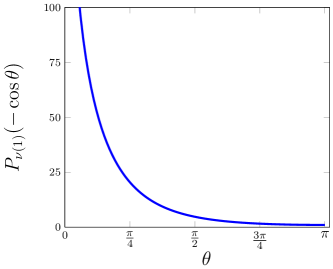
Figure 1: The LegendreP function $P_{\nu(k)}(-\cos\theta)$, for $\theta\in(0,\pi]$ and $k=1$

We also recall that $P_{\nu}$ is well-defined for all $\nu\in\mathbb{C}$, whereas $Q_{\nu}$ is well-defined for $\nu\not=0,-1,-2,...$.

On $\mathcal{S}$, from (5) we obtain

$$\nu(k):=\frac{-1+\sqrt{1-4k^{2}}}{2}.$$

If $0<k^{2}<\frac{1}{4}$ then $\nu\in(-1,0)$. If $k^{2}\geq\frac{1}{4}$ then

$$\nu(k):=\frac{-1+i\sqrt{4k^{2}-1}}{2}.$$

We observe that since $k^{2}>0$, $\nu(k)\notin\mathbb{Z}$. Moreover, if $k>\frac{1}{2}$ then $Im(\nu)\not=0$. This is the regime in which we shall work, and in what follows we shall make this assumption on $k$. Recall that in $k^{2}=bigO(1/\Delta t)$ in the our applications of interest.

A further substitution allows us to write (5) as a hypergeometric equation, (see, e.g., Section 7.3, lebedev ). This in turn allows us to write the solution of $\mathcal{D}_{k}(u)=0$ as

$$u(r_{0}(\theta)) =P_{\nu(k)}(-\cos(\theta))=\tensor[_{2}]{F}{{}_{1}}\left(-\nu(k),\nu(k)+1;1;\frac{4-r_{0}^{2}(\theta)}{2}\right)$$

$$=\tensor[_{2}]{F}{{}_{1}}\left(-\nu(k),\nu(k)+1;1;\frac{1+\cos(\theta)}{2}\right).$$

Here, $\tensor[_{2}]{F}{{}_{1}}(a,b;c;z)$ is a hypergeometric function. Since the argument $\frac{1+\cos(\theta)}{2}$ lies between $-1$ and $1$, and $a+b=1$, the representation in terms of the hypergeometric function is also known as the Ferrers’ function of the first kind, fatAbramowitz .

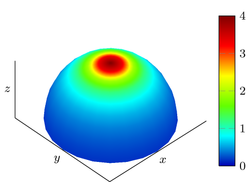
Figure 2: $G_{1}(x,x_{0})$ when $x_{0}=(0,0,1)^{T}$. The singularity at the north pole is logarithmic. Only the top hemisphere is shown here for purpose of illustration

A more (computationally) convenient representation is in terms of the conical or Mehler functions (Section 8.5 in lebedev ). The conical function $P_{-\frac{1}{2}+i\tau}(z)$ of order $\tau\in\mathbb{R}$ solves the equation

$$(1-z^{2})\,w^{\prime\prime}-2zw^{\prime}-\left(\tau^{2}+\frac{1}{4}\right)\,w=0.$$

In our specific case, we would pick $\tau=\tau(k)$ such that $\tau^{2}+\frac{1}{4}=k^{2}=-\nu(\nu+1).$ It follows that

$$\tau:=\frac{\sqrt{4k^{2}-1}}{2}\Rightarrow\nu=-\frac{1}{2}+i\tau,$$

and the solution of $\mathcal{D}_{k}(u)=0$ is $P_{\nu}(-\cos(\theta))=P_{-\frac{1}{2}+i\tau}(-\cos(\theta)).$ The calculations above lead us then to the following definition:

Definition 1

The fundamental solution for the Yukawa-Beltrami operator $-\bigtriangleup_{\mathcal{S}}+k^{2}$ for points $x,x_{0}$ on the surface of the unit sphere is

$$G_{k}(x,x_{0}) :=C_{k}P_{\nu}\left(-<x,x_{0}>\right)$$

$$:=C_{k}P_{\nu}\left(\frac{\|x-x_{0}\|^{2}}{2}-1\right)$$ (6a)

$$=C_{k}\,\tensor[_{2}]{F}{{}_{1}}\left(-\nu,\nu+1;1;\frac{1+<x,x_{0}>}{2}\right)$$ (6b)

$$=C_{k}P_{-\frac{1}{2}+i\tau}\left(<x,x_{0}>\right),$$ (6c)

where $\nu:=\frac{-1+i\sqrt{4k^{2}-1}}{2}$, $k>1/2$, and

$$C_{k}=-\frac{1}{4\sin(\nu\pi)}=\frac{1}{4\cosh(\frac{\pi}{2}\sqrt{4k^{2}-1})}.$$ (7)

(See Figure 2 for a visualization of $G_{1}(x,x_{0})$.) We mention here that the specific choice of $C_{k}$ is motivated by the calculations performed while deriving a representation formula in Section 2.2. We will see that $C_{k}$ is well-defined with our assumption that $k>1/2$.

2.1 Properties of the fundamental solution of the Yukawa-Beltrami operator

Before we embark on the definition and analysis of boundary integral operators, we examine some properties of the fundamental solution $G_{k}$ defined in Definition 1. We shall use either the representation (6a), (6b), or (6c) as convenient. We first observe that the fundamental solution is symmetric in its arguments, $G_{k}(x,x_{0})=G_{k}(x_{0},x)$. Next, by noting the expansion for the conical functions as lebedev

$$P_{-\frac{1}{2}+i\tau}(\cos(t)) =1+\frac{4\tau^{2}+1}{2^{2}}\sin^{2}(t/2)+\frac{(4\tau^{2}+1)(4\tau^{2}+3^{2})}{2^{2}4^{2}}\sin^{4}(t/2)+\cdots,$$

for $0\leq t\leq\pi$, we see that $G_{k}(x,x_{0})$ does not change sign for all $x,x_{0}\in\mathcal{S},x\neq x_{0}$, provided $k$ is fixed.

Next, we examine the asymptotic behaviour as $x\rightarrow x_{0}$. In this case, it is convenient to work with (6a). Setting $\mu=0$ in 14.8.1 of fatAbramowitz (or using 7.5.5 in lebedev ), we have the asymptotic behaviour

$$\lim_{t\rightarrow 1^{-}}P_{\nu}(t) =\frac{1}{\Gamma(1)}=1.$$ (8)

Next, following fatAbramowitz , as $t\rightarrow 1^{-}$,

$$Q_{\nu}(t)=\frac{1}{2}\log\left(\frac{2}{1-t}\right)-\gamma-\psi(\nu+1)+\mathcal{O}(1-t),\>\nu\neq-1,-2,...$$

where $\psi(x)$ is the digamma function, $\gamma=0.5772\ldots$ is Euler’s constant, and $Q_{\nu}$ is the other linearly independent solution of Legendre’s equation (5). For subsequent use, we denote

$$R(\nu):=\frac{1}{2}\log(2)-\gamma-\psi(\nu+1),$$

and therefore for $t$ close to $1$,

$$Q_{\nu}(t)=-\frac{1}{2}\log(1-t)+R(\nu)+\mathcal{O}(1-t),\>\nu\neq-1,-2,...$$ (9)

Now, as $x\rightarrow x_{0}$ on the surface of the sphere, using (6a) we have

$$\lim_{x\rightarrow x_{0}}G_{k}(x,x_{0})=C_{k}\lim_{x\rightarrow x_{0}}P_{\nu(k)}\left(-<x,x_{0}>\right)=C_{k}\lim_{t\rightarrow 1^{-}}P_{\nu(k)}\left(-t\right).$$

We cannot immediately use (8). Instead, we must use the connection formula 14.9.10 in fatAbramowitz (again setting $\mu=0$):

$$\frac{2}{\pi}\sin(\nu\pi)Q_{\nu}(t)=\cos(\nu\pi)P_{\nu}(t)-P_{\nu}(-t).$$ (10)

Combining (10) with (8) and (9), we obtain

$$\lim_{x\rightarrow x_{0}}G_{k}(x,x_{0}) =\lim_{x\rightarrow x_{0}}C_{k}P_{\nu}(-<x,x_{0}>)$$

$$=\lim_{x\rightarrow x_{0}}C_{k}\left(\cos(\nu\pi)P_{\nu}(<x,x_{0}>)-\frac{2}{\pi}\sin(\nu\pi)Q_{\nu}(<x,x_{0}>)\right)$$

$$=C_{k}\cos(\nu\pi)$$

$$\quad-\frac{2C_{k}}{\pi}\sin(\nu\pi)\lim_{x\rightarrow x_{0}}\left(-\frac{1}{2}\log(1-<x,x_{0}>)+R(\nu)+\mathcal{O}(1-<x,x_{0}>)\right)$$

$$=\frac{C_{k}\sin(\nu\pi)}{\pi}\lim_{x\rightarrow x_{0}}\log(1-<x,x_{0}>)+C_{k}\left[\cos(\nu\pi)-2\frac{\sin(\nu\pi)}{\pi}R(\nu)\right].$$ (11)

Therefore, as $x\rightarrow x_{0}$ $G_{k}(x,x_{0})$ possesses a logarithmic singularity (recall that $\nu$ is not an integer). At this point, we could predict a value for $C_{k}$ so that the strength the singularity is consistent with that for the Laplace-Beltrami gemmrich . However, we compute $C_{k}$ rigorously below.

It is also useful to document the relation, obtained using recurrence relations for the LegendreP function (Section 14.10.4 in fatAbramowitz ):

$$(1-z^{2})P^{\prime}_{\nu}(z)=(-\nu-1)P_{\nu+1}(z)+(\nu+1)zP_{\nu}(z).$$

Suppose, again without loss of generality, that $x_{0}$ is the North Pole. Let $x=x(\theta,\phi)$. Then, $G_{k}(x,x_{0})=C_{k}P_{\nu}(-\cos(\theta))$, and

$$\frac{d}{d\theta}P_{\nu}(-\cos(\theta))=(\nu+1)(\sin\theta)\left(\frac{P_{\nu+1}(-z)+zP_{\nu}(-z)}{z^{2}-1}\right)|_{z=\cos(\theta)}.$$ (12)

Now, using (12),

$$\underline{\mbox{curl}}_{\mathcal{S}}G_{k}(x,x_{0}) =-C_{k}\frac{\partial}{\partial\theta}\left[P_{\nu(k)}(-\cos(\theta))\right]\vec{e}_{\varphi}$$

$$=-C_{k}(\nu+1)\frac{\sin(\theta)}{\cos^{2}\theta-1}\left[P_{\nu+1}(-z)+zP_{\nu}(-z)\right]|_{z=\cos(\theta)}\vec{e}_{\varphi}.$$

Since the line element on the surface of the sphere is given by

$$\vec{t}(x(\varphi,\theta))\cdot ds_{x(\varphi,\theta)}=d\theta\,\vec{e}_{\theta}\,+\,\sin\theta d\varphi\,\vec{e}_{\varphi},$$

we obtain that

$$\underline{\mbox{curl}}_{\mathcal{S}}G_{k}(x,x_{0})\cdot\vec{t} =C_{k}(\nu+1)\left[P_{\nu+1}(-z)+zP_{\nu}(-z)\right]|_{z=\cos(\theta)}d\phi=:F(\theta)d\phi.$$ (13)

The term $F(\theta)=C_{k}(\nu+1)\left[P_{\nu+1}(-z)+zP_{\nu}(-z)\right]|_{z=\cos(\theta)}$ will be important in subsequent sections, and is related to the kernel of the second layer operator. (We shall define this operator carefully later.) For now, however, we are interested in the limit of $F(\theta)$ as the point $x\rightarrow x_{0}$, that is, as $\theta\rightarrow 0^{+}$.

Lemma 1

Let $F(\theta)$ be as defined in (13). Then $\lim_{\theta\rightarrow 0^{+}}F(\theta)=\frac{2}{\pi}C_{k}\sin(\nu\pi)$.

Proof

Using (10), the term in the square bracket of

$$F(\theta)=C_{k}(\nu+1)\left[P_{\nu+1}(-z)+zP_{\nu}(-z)\right]|_{z=\cos(\theta)},$$

can be simplified. Denoting $\cos(\theta)=z$,

$$P_{\nu+1}(-z)+zP_{\nu}(-z) =-\frac{2}{\pi}\sin\left((\nu+1)\pi\right)Q_{\nu+1}(z)+\cos((\nu+1)\pi)P_{\nu+1}(z)$$

$$\qquad+z\left[-\frac{2}{\pi}\sin(\nu\pi)Q_{\nu}\left(z\right)+\cos(\nu\pi)P_{\nu}\left(z\right)\right]$$

$$=-\frac{2}{\pi}\left[z\sin(\nu\pi)Q_{\nu}\left(z\right)+\sin\left((\nu+1)\pi\right)Q_{\nu+1}\left(z\right)\right]$$

$$\qquad+\left[\cos((\nu+1)\pi)P_{\nu+1}\left(z\right)+z\cos(\nu\pi)P_{\nu}\left(z\right)\right]$$

$$=-\frac{2}{\pi}\sin(\nu\pi)\left[zQ_{\nu}\left(z\right)-Q_{\nu+1}\left(z\right)\right]+\cos(\nu\pi)\left[-P_{\nu+1}\left(z\right)+zP_{\nu}\left(z\right)\right].$$ (14)

As $x\rightarrow x_{0}$, i.e., as $\theta\rightarrow 0^{+}$, clearly $z=\cos(\theta)\rightarrow 1^{-}$. Recall that in this limit, $P_{\nu}(z)\rightarrow 1.$ Therefore, the terms involving the LegendreP functions of the first kind in (14) behave as

$$\lim_{z\rightarrow 1^{-}}\cos(\nu\pi)\left[-P_{\nu+1}(z)+zP_{\nu}(z)\right]=0.$$ (15)

We can use (8) to compute the limit of the term involving the Legendre functions of the second kind in (14):

$$\lim_{z\rightarrow 1^{-}}-\frac{2}{\pi}\sin(\nu\pi)\left[zQ_{\nu}\left(z\right)-Q_{\nu+1}\left(z\right)\right] =-\frac{2}{\pi}\sin(\nu\pi)\left[\psi(\nu+2)-\psi(\nu+1)\right]$$

$$=-\frac{2}{\pi(\nu+1)}\sin(\nu\pi).$$ (16)

Putting together (15), (16), and (13), we have

$$\lim_{\theta\rightarrow 0^{+}}F(\theta)=\lim_{z\rightarrow 1-}C_{k}(\nu+1)\left[P_{\nu+1}(-z)+zP{\nu}(-z)\right]=C_{k}\frac{2}{\pi}\sin(\nu\pi).$$ (17)

∎

Observe that setting $C_{k}=-\frac{1}{4\sin(\nu\pi)}$, that is, using exactly the constant defined in (7) in the definition of $G_{k}(x,x_{0})$, we have $\lim_{\theta\rightarrow 0^{+}}F(\theta)=\frac{1}{2\pi}.$

2.2 Representation formula

Let $\Omega$ and $\Omega^{c}:=\mathcal{S}\setminus{\overline{\Omega}}$ be a simply-connected submanifold and its complement on the sphere. We can then derive a representation formula in terms of the fundamental solution $G_{k}(x,x_{0})$ of the previous section.

Proposition 1

Every sufficiently smooth function $u\in C^{2}(\Omega)\cap C^{1}(\overline{\Omega})$ satisfies the representation formula

$$-\int\limits_{\Omega}G_{k}(x,x_{0})\left[\bigtriangleup_{\mathcal{S}}u(x)-k^{2}u(x)\right]\,d\sigma_{x} -\int\limits_{{\Gamma}}G_{k}(x,x_{0})\underline{\mbox{curl}}_{\mathcal{S}}u(x)\cdot\vec{t}(x)ds_{x}$$

$$+\int\limits_{{\Gamma}}u(x)\,\underline{\mbox{curl}}_{{\mathcal{S}}}G_{k}(x,x_{0})\cdot\vec{t}(x)ds_{x} =\left\{\begin{array}[]{ll}u(x_{0})&\mbox{ if $x_{0}\in\Omega$},\\ 0&\mbox{ if $x_{0}\in{\Omega}_{c}$}.\end{array}\right.$$ (20)

Proof

We let $x\in\Omega$, and $x_{0}$ be a point either in $\Omega$ or $\Omega^{c}$. We proceed by examining the two possible cases.

Case 1: $x_{0}\in\Omega^{c}$. In this situation, the fundamental solution $G_{k}(x,x_{0})$ satisfies the Yukawa-Beltrami equation point-wise at all $x\in\Omega$. Since $x\neq x_{0}$, $G_{k}(x,x_{0})$ is a smooth function and we can therefore use Green’s second identity (4) with $v(x)$ replaced by $G_{k}(x,x_{0})$. Since $x_{0}\not\in\Omega$ all the integrals involved are bounded, and

$$\int\limits_{\Omega}u(x)(\bigtriangleup_{\mathcal{S}}G_{k}(x,x_{0})-k^{2}G_{k}(x,x_{0}))\,d\sigma_{x}=0.$$

Therefore, using (4) we have

$$0 =-\int\limits_{\Omega}G_{k}(x,x_{0})\left(\bigtriangleup_{\mathcal{S}}u(x)-k^{2}u(x)\right)\,d\sigma_{x}$$

$$-\int\limits_{{\Gamma}}G_{k}(x,x_{0})\,\underline{\mbox{curl}}_{\mathcal{S}}u(x)\cdot\vec{t}(x)ds_{x}+\int\limits_{{\Gamma}}u(x)\,\underline{\mbox{curl}}_{{\mathcal{S}}}G_{k}(x,x_{0})\cdot\vec{t}(x)ds_{x}.$$

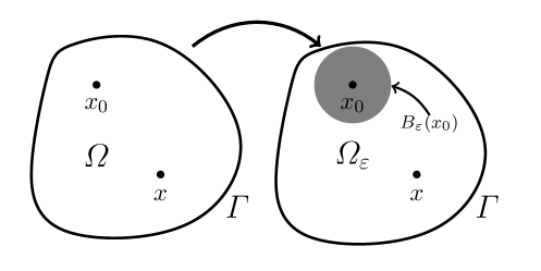
Figure 3: The points $x,x_{0}$ belong to $\Omega$. We denote by $\Omega_{\varepsilon}:=\Omega\setminus B_{\varepsilon}(x_{0})$

Case 2: $x_{0}\in\Omega$. In this situation we cannot directly use Green’s second identity, since the fundamental solution has a logarithmic singularity when $x=x_{0}$. Instead, we first define the $\varepsilon$-neighbourhood of $x_{0}$, $B_{\varepsilon}(x_{0}):=\{y\in{\mathcal{S}}:\,|y-x_{0}|\,<\,\varepsilon\}$. We choose $\varepsilon>0$ small enough such that $B_{\varepsilon}(x_{0})\subset\Omega$ (see Figure 3). We then set ${\Omega}_{\varepsilon}:=\Omega\setminus B_{\varepsilon}(x_{0})$. For $x\in\Omega_{\varepsilon}$, once again $G_{k}(x,x_{0})$ satisfies the Yukawa-Beltrami equation exactly. The second Green’s formula for $\Omega_{\varepsilon}$ with $v(x)=G_{k}(x,x_{0})$ yields:

$$-\int\limits_{\Omega_{\varepsilon}}G_{k}(x,x_{0})\,(\bigtriangleup_{\mathcal{S}} u(x)-k^{2}u(x))\,d\sigma_{x}=\int\limits_{\Gamma}[G_{k}(x,x_{0})\,\underline{\mbox{curl}}_{\mathcal{S}}u(x)-u(x)\,\underline{\mbox{curl}}_{\mathcal{S}}G_{k}(x,x_{0})]\cdot\vec{t}(x)ds_{x}$$

$$+\int\limits_{\partial B_{\varepsilon}(x_{0})}[G_{k}(x,x_{0})\,\underline{\mbox{curl}}_{\mathcal{S}}u(x)-u(x)\,\underline{\mbox{curl}}_{\mathcal{S}}G_{k}(x,x_{0})]\cdot\vec{t}(x)ds_{x}.$$ (21)

We shall discuss each of these terms. We first note that since $x_{0}\in\Omega$, the integrals over $\Gamma$ in (21) are well-defined. So we must examine the volume integral over $\Omega_{\varepsilon}$ and the integrals over $\partial B_{\varepsilon}$. For ease of exposition and without loss of generality, we take $x_{0}=(0,0,1)$. The curve $\partial B_{\varepsilon}$ is then fully described by the latitude $\theta_{\varepsilon}$. In this case, if $x\in\partial B_{\varepsilon}$, then $<x,x_{0}>=\cos(\theta_{\varepsilon})$, and $G_{k}(x,x_{0})=C_{k}P_{\nu(k)}\left(-<x,x_{0}>\right)=C_{k}P_{\nu(k)}\left(-\cos(\theta_{\varepsilon})\right).$ Therefore, since $\cos(\theta_{\varepsilon})=1-\theta^{2}_{\varepsilon}/2+\cdots$, we can use the asymptotic result (11) to compute

$$\int\limits_{\partial B_{\varepsilon}}|G_{k}(x,x_{0})\,|ds_{x} \leq\int_{0}^{2\pi}|C_{k}P_{\nu(k)}(-\cos\theta_{\varepsilon})\,\sin\theta_{\varepsilon}|\,d\varphi$$

$$=C_{k}|\sin\theta_{\varepsilon}||P_{\nu(k)}(-\cos\theta_{\varepsilon})|2\pi$$

$$=2\pi|\sin\theta_{\varepsilon}|C_{k}\left(\cos(\nu\pi)P_{\nu(k)}(\cos\theta_{\varepsilon})-\frac{2}{\pi}\sin(\nu\pi)Q_{\nu}(\cos\theta_{\varepsilon})\right)$$

$$\rightarrow 0\quad\mbox{ (as $\varepsilon\rightarrow 0$)},$$

where the limit holds since the singularity of $P_{\nu(k)}$ is only logarithmic. We can therefore estimate the first integral over $\partial B_{\varepsilon}$ in (21) as

$$\left|\int\limits_{\partial B_{\varepsilon}}G_{k}(x,x_{0})\,\underline{\mbox{curl}}_{\mathcal{S}}u(x)\cdot\vec{t}(x)\,ds_{x}\right|\,\leq\,\|\underline{\mbox{curl}}_{\mathcal{S}}u\|_{L^{\infty}}\,\int\limits_{\partial B_{\varepsilon}}|G_{k}(x,x_{0})|\,ds_{x}\rightarrow 0,\,\mbox{as}\,\varepsilon\rightarrow 0.$$

To analyse the second contribution along $\partial B_{\varepsilon}$ in (21), we again assume $x_{0}=(0,0,1)$. Using (13) we deduce that (note the orientation of $\partial B_{\varepsilon}$)

$$-\int\limits_{\partial B_{\varepsilon}}[u(x) \underline{\mbox{curl}}_{\mathcal{S}}G(x,x_{0})\cdot\vec{t}(x)]ds_{x}$$

$$=\frac{C_{k}(\nu+1)\sin^{2}\theta_{\varepsilon}}{\cos^{2}\theta_{\varepsilon}-1}\left[P_{\nu+1}(-\cos\theta_{\varepsilon})+(\cos\theta_{\varepsilon})P_{\nu}(-\cos\theta_{\varepsilon})\right]\int_{2\pi}^{0}u(\varphi,\theta_{\varepsilon})\,d\varphi$$

$$=C_{k}(\nu+1)\left[P_{\nu+1}(-\cos\theta_{\varepsilon})+(\cos\theta_{\varepsilon})P_{\nu}(-\cos\theta_{\varepsilon})\right]\int_{0}^{2\pi}u(\varphi,\theta_{\varepsilon})\,d\varphi.$$ (22)

Combining (15), (16) and (2.2) and using the continuity of $u$, we have

$$-\lim_{\varepsilon\rightarrow 0}\int\limits_{\partial B_{\varepsilon}}u(x) [\underline{\mbox{curl}}_{\mathcal{S}}G(x,x_{0})\cdot\vec{t}(x)]ds_{x}=-4C_{k}\sin(\nu\pi)u(x_{0})=u(x_{0}).$$

Note that $C_{k}=-\frac{1}{4\sin(\nu\pi)}$ is chosen precisely to be this value in (7) to ensure this integral, in the limit, is $u(x_{0})$.

We finally observe that since $u$ is assumed to be smooth enough,

$$\left|\int\limits_{\Omega}G_{k}(x,x_{0})\,(\bigtriangleup_{\mathcal{S}}u(x)-k^{2}u(x))\,d\sigma_{x}\right|\, \leq\,\|\bigtriangleup_{\mathcal{S}}\,u-k^{2}u\|_{L^{\infty}(\Omega)}\int\limits_{\Omega}|G_{k}(x,x_{0})|\,d\sigma_{x}\,$$

$$\leq\|\bigtriangleup_{\mathcal{S}}\,u-k^{2}u\|_{L^{\infty}(\Omega)}M,$$

where $M$ is a constant which depends on the volume of $\Omega$. Specifically, since $P_{\nu}(k)(-t)$ is smooth away from the (logarithmic) singularity at $t=1$, we have

$$M:=\int\limits_{\Omega}|G_{k}(x,x_{0})|\,d\sigma_{x}=\int_{B_{\varepsilon}(x_{0})}|G_{k}(x,x_{0})|\,d\sigma_{x}+M_{1}.$$

The first integral is bounded since the logarithm is integrable over ${B_{\varepsilon}(x_{0})}$, and $M_{1}$ is some finite constant depending on the area of $\Omega$. Hence $M$ is a finite positive constant depending on $\Omega$ and

$$\lim_{\varepsilon\rightarrow 0}\int\limits_{\Omega_{\varepsilon}}G_{k}(x,x_{0})\,(\bigtriangleup_{\mathcal{S}}u(x)-k^{2}u(x))\,d\sigma_{x}=\int\limits_{\Omega}G_{k}(x,x_{0})\,(\bigtriangleup_{\mathcal{S}}u(x)-k^{2}u(x))\,d\sigma_{x}.$$

Therefore, taking limits in (21) proves the result.

∎

3 Layer potentials and boundary integral operators

Now that we have a convenient parametrix $G_{k}(x,x_{0})$ defined in Definition 1 for the Yukawa-Beltrami equation and a representation formula (1), we can define convenient layer potentials which in turn will be used to reduce the boundary value problem (2) over the domain $\Omega$ to a boundary integral equation over $\Gamma=\partial\Omega$.

3.1 Single- and double-layer potentials

We define the following two layer potentials.

• The single-layer potential with sufficiently smooth density function $\sigma$:

  $$(\widetilde{V_{k}}\sigma)(x):=\int\limits_{\Gamma}G_{k}(x,y)\,\sigma(y)\,ds_{y},\quad\mbox{for $x\notin\Gamma$};$$ (23)

• and the double-layer potential with sufficiently smooth density function $\mu$:

  $$(\widetilde{W_{k}}\mu)(x):=\int\limits_{\Gamma}\mu(y)\,[\underline{\mbox{curl}}_{\mathcal{S}}G_{k}(x,y)\cdot\vec{t}(y)]\,ds_{y},\quad\mbox{for $x\notin\Gamma$},$$ (24)

We wish to point out here that the form of the double-layer potential above is equivalent to the, perhaps, more familiar form:

$$(\widetilde{W_{k}}\mu)(x):=-\int\limits_{\Gamma}\mu(y)\frac{\partial\,}{\partial n_{y}}G_{k}(x,y)\,ds_{y},\quad\mbox{for $x\notin\Gamma$}.$$ (25)

where $n_{y}$ is the outward pointing normal to $\Gamma$ at the point $y$ lying in a tangent plane to $\mathcal{S}$. See kro:nig2013 for a more detailed discussion on this point.

By Proposition 1, every solution to the homogeneous Yukawa-Beltrami equation can be written as the sum of a single- and a double-layer potential. This is the starting point for the so-called direct boundary integral approach. However, for the purpose of this paper we follow the layer ansatz based on the following observation.

For $x\notin\Gamma,x\in\Omega$, the single-layer potential in (23) satisfies:

$$(-\bigtriangleup_{\mathcal{S}}+k^{2})(\widetilde{V_{k}}\sigma)(x) =(-\bigtriangleup_{\mathcal{S}}+k^{2})\int\limits_{\Gamma}G_{k}(x,y)\,\sigma(y)\,ds_{y}$$

$$=\int\limits_{\Gamma}(-\bigtriangleup_{\mathcal{S}}+k^{2})G_{k}(x,y)\,\sigma(y)\,ds_{y}=\,0.$$

Hence, we may find the general solution of the Dirichlet boundary value problem (2) in terms of a single-layer potential

$$u(x) =\int\limits_{\Gamma}G_{k}(x,y)\,\sigma(y)\,ds_{y}.$$

We would then need to calculate the unknown density $\sigma$.

Similarly, the double-layer potential in (24) satisfies the Yukawa-Beltrami equation for $x\in\Omega,x\notin\Gamma$

$$(-\bigtriangleup_{\mathcal{S}}+k^{2})(\widetilde{W}\mu)(x) =(-\bigtriangleup_{\mathcal{S}}+k^{2})\int\limits_{\Gamma}\mu(y)\,[\underline{\mbox{curl}}_{\mathcal{S}}G(x,y)\cdot\vec{t}(y)]\,ds_{y}$$

$$=\int\limits_{\Gamma}\mu(y)[(\bigtriangleup_{\mathcal{S}}-k^{2})\,\underline{\mbox{curl}}_{\mathcal{S}}\,G(x,y)\cdot\vec{t}(y)]\,ds_{y}$$

$$=\int\limits_{\Gamma}\mu(y)[\underline{\mbox{curl}}_{\mathcal{S}}\,(\bigtriangleup_{\mathcal{S}}-k^{2})G(x,y)\cdot\vec{t}(y)]\,ds_{y}=0.$$

We might thus also try to look for the solution to (2) in the form of a double-layer.

3.2 Jump relations for the layer potentials

In the previous section, we have only defined the layer potentials for $x$ away from the boundary curve. However, in order to align the operators with the given Dirichlet data along $\Gamma$, we need to investigate their behavior in the limit as $x$ approaches $\Gamma$. Similarly, if one is interested in solving the Neumann problem in which the tangential component of the vectorial surface rotation is prescribed along $\Gamma$, one has to investigate the limit features of this quantity for the layer potentials. In both cases, there will be certain jump relations across the curve $\Gamma$. For the purpose of this paper however, we will restrict ourselves to the Dirichlet case. First, consider the single-layer potential with density $\sigma$ for $x\notin\Gamma$:

$$(\widetilde{V_{k}}\sigma)(x) =\int\limits_{\Gamma}G_{k}(x,y)\,\sigma(y)\,ds_{y}$$

$$=C_{k}\int\limits_{\Gamma}P_{\nu(k)}(-<x,y>)\,\sigma(y)\,ds_{y}.$$

The following Lemma describes the limit behavior of the single-layer potential.

Lemma 2

Let $\widetilde{V_{k}}$ be the single-layer potential defined in (23). For $x_{0}\in\Gamma$ we have:

$$(V\sigma)(x_{0}) :=\lim\limits_{\begin{subarray}{c}x\to x_{0}\\ x\in\Omega\end{subarray}}\,(\widetilde{V_{k}}\sigma)(x)=\int\limits_{\Gamma}G_{k}(x_{0},y)\,\sigma(y)\,ds_{y}$$

as a weakly singular line integral and hence $(\widetilde{V_{k}}\sigma)$ is continuous across $\Gamma$.

Proof

Fix an arbitrary $\varepsilon>0$. Let $x_{0}\in\Gamma$ be fixed, and $x\in\Omega$ satisfy $|x-x_{0}|<\varepsilon$. Introduce the notation

$$C_{\varepsilon,\leq}:=\{y\in\Gamma,\|y-x_{0}\|\leq\varepsilon\},\qquad C_{\varepsilon,>}:=\{y\in\Gamma,\|y-x_{0}\|>\varepsilon\}.$$

Then, if we define

$$I_{\varepsilon}(x) :=\int\limits_{\Gamma}G_{k}(x,y)\,\sigma(y)\,ds_{y}-\int_{C_{\varepsilon,>}}G_{k}(x_{0},y)\,\sigma(y)\,ds_{y},$$

we can easily show

$$I_{\varepsilon} =\int_{C_{\varepsilon,>}}\left[G_{k}(x,y)\,-\,G_{k}(x_{0},y)\right]\,\sigma(y)\,ds_{y}+\int_{C_{\varepsilon,\leq}}G_{k}(x,y)\,\sigma(y)\,ds_{y}.$$ (26)

The first integral in (26) vanishes in the limit as $x\rightarrow x_{0}$ since $P_{\nu(k)}(1-<x,x_{0}>)$ is continuous away from $<x,x_{0}>=1$, i.e. where $x=x_{0}$. That is,

$$\lim\limits_{x\to x_{0}}\int_{C_{\varepsilon,>}}\left[G_{k}(x,y)\,-\,G_{k}(x_{0},y)\right]\,\sigma(y)\,ds_{y}=0.$$

The second term in (26) can be bound in terms of the density $\sigma$:

$$\left|\int_{C_{\varepsilon,\leq}}G_{k}(x,y)\,\sigma(y)\,ds_{y}\,\right|\,\leq\,\|\sigma\|_{L_{\infty}(\Gamma)}\int_{C_{\varepsilon,\leq}}\left|G_{k}(x,y)\right|\,ds_{y}.$$

To finish the proof, note that we can estimate

$$\int_{C_{\varepsilon,\leq}}\left|G_{k}(x,y)\right|\,ds_{y}\,\leq\,\int\limits_{\begin{subarray}{c}y\in\Gamma\\ |y-x|\leq 2\varepsilon\end{subarray}}\left|G_{k}(x,y)\right|\,ds_{y}\buildrel x\rightarrow x_{0}\over{\longrightarrow}\int\limits_{\begin{subarray}{c}y\in\Gamma\\ |y-x_{0}|\leq 2\varepsilon\end{subarray}}\left|G_{k}(x_{0},y)\right|\,ds_{y}\buildrel\varepsilon\rightarrow 0\over{\longrightarrow}0.$$

As before, the final limit holds since $G_{k}(x_{0},y)$ has a logarithmic singularity at $y=x_{0}$. Putting these estimates together, we see that $\displaystyle\lim_{\varepsilon\rightarrow 0}\lim_{x\rightarrow x_{0}}I_{\varepsilon}(x)=0$, which proves the assertion.

∎

The case of the double-layer potential is slightly more involved. We anticipate that, just as for the Laplace-Beltrami double-layer potential gemmrich , the Yukawa-Beltrami double-layer will possess a jump across the boundary of a domain. Indeed, since $G_{k}(x,x_{0})$ has a logarithmic singularity, the estimates follow the same argument as for the Laplace-Beltrami. The details of the calculation are cumbersome, but the overall strategy is that of Section 8.2 in hackbusch .

Lemma 3

Let $\widetilde{W_{k}}$ be the double-layer potential defined in (24), and let $\gamma_{0}^{\Omega}$ (resp. $\gamma_{0}^{\Omega^{c}})$ denote the trace operator on $\Gamma$, with traces from inside (respectively outside) $\Omega$. For $x_{0}\in\Gamma$ we have:

$$(\gamma^{\Omega^{c}}_{0}\widetilde{W_{k}}\mu)(x_{0})=\lim\limits_{\begin{subarray}{c}x\to x_{0}\\ x\in\Omega^{c}\end{subarray}}\,(\widetilde{W_{k}}\mu)(x)=(K\mu)(x_{0})\,+\,\left(1-\frac{\alpha(x_{0})}{2\pi}\right)\,\mu(x_{0}),$$

where $\alpha(x_{0})$ represents the interior (with respect to $\Omega^{c}$) angle of $\Gamma$ at $x_{0}$. For a smooth curve, $\alpha=\pi$. The double-layer operator $K$ is defined via the Cauchy principle value:

$$(K\mu)(x_{0}) =\lim_{\varepsilon\rightarrow 0}\,(K_{\varepsilon}\mu)(x_{0})\quad\mbox{where}\qquad(K_{\varepsilon}\mu)(x_{0}) :=\int\limits_{y\in C_{\epsilon,\geq}}\mu(y)\,\left[\underline{\mbox{curl}}_{\mathcal{S}}\,G_{k}(x_{0},y)\cdot\vec{t}(y)\right]\,ds_{y}.$$

Hence the double-layer potential satisfies:

$$\left[(\gamma_{0}\widetilde{W}_{k}\mu)\right]_{\Gamma}:=(\gamma^{\Omega^{c}}_{0}\widetilde{W}_{k}\mu)+(\gamma^{\Omega}_{0}\widetilde{W_{k}}\mu)=\mu,$$

where we tacitly assumed the orientation of the tangential vector $\vec{t}$ along $\Gamma$ to be in accordance with the orientation of $\Omega^{c}$ in the sense of Stoke’s theorem.

Proof

We provide only a sketch of the proof. Given $\varepsilon\,>\,0$, let $x\in\Omega^{c}$ with $\|x-x_{0}\|<\varepsilon$. We use the same notation for $C_{\epsilon,\geq}$ and $C_{\epsilon,<}$ introduced earlier. Then, for fixed $\varepsilon>0$,

$$(\widetilde{W_{k}}\mu)(x)-(K_{\varepsilon}\mu)(x_{0})=\int_{C_{\varepsilon,\geq}}\mu(y)\left[\underline{\mbox{curl}}_{\mathcal{S}}\,G_{k}(x,y)\,-\,\underline{\mbox{curl}}_{\mathcal{S}}\,G_{k}(x_{0},y)\right]\cdot\vec{t}(y)\,ds_{y}$$

$$+\int_{C_{\varepsilon,<}}\mu(y)\,\underline{\mbox{curl}}_{\mathcal{S}}\,G_{k}(x,y)\cdot\vec{t}(y)\,ds_{y}.$$ (27)

We note that the integrand of $\int_{C_{\varepsilon,\geq}}\mu(y)\left[\underline{\mbox{curl}}_{\mathcal{S}}\,G_{k}(x,y)\,-\,\underline{\mbox{curl}}_{\mathcal{S}}\,G_{k}(x_{0},y)\right]\cdot\vec{t}(y)\,ds_{y}$ is continuous in $x$ away from $x_{0}$, and therefore

$$\lim_{x\rightarrow x_{0}}\int_{C_{\varepsilon,\geq}}\mu(y)\left[\underline{\mbox{curl}}_{\mathcal{S}}\,G_{k}(x,y)\,-\,\underline{\mbox{curl}}_{\mathcal{S}}\,G_{k}(x_{0},y)\right]\cdot\vec{t}(y)\,ds_{y}=0.$$

The integral over $C_{\varepsilon,<}$ in (27) can be rewritten as

$$\int_{C_{\varepsilon,<}}\mu(y)\,\underline{\mbox{curl}}_{\mathcal{S}}\,G_{k}(x,y)\cdot\vec{t}(y)\,ds_{y}= \int_{C_{\varepsilon,<}}\left[\mu(y)-\mu(x_{0})\right]\,\underline{\mbox{curl}}_{\mathcal{S}}\,G_{k}(x,y)\cdot\vec{t}(y)\,ds_{y}$$

$$+\mu(x_{0}) \int_{C_{\varepsilon,<}}\underline{\mbox{curl}}_{\mathcal{S}}\,G_{k}(x,y)\cdot\vec{t}(y)\,ds_{y}.$$ (28)

For the first integral on the right hand side of (28), using Lemma 4, we have the estimate (for a fixed $x$)

$$\left|\int_{C_{\varepsilon,<}}\left[\mu(y)-\mu(x_{0})\right]\,\underline{\mbox{curl}}_{\mathcal{S}}\,G_{k}(x,y)\cdot\vec{t}(y)\,ds_{y}\right|$$

$$\qquad\leq\sup_{y\in C_{\varepsilon,<}}|\mu(y)-\mu(x_{0})|\int_{C_{\varepsilon,<}}\left|\underline{\mbox{curl}}_{\mathcal{S}}\,G_{k}(x,y)\cdot\vec{t}(y)\right|\,ds_{y}$$

$$\qquad\leq M\,\cdot\mbox{length $(C_{\varepsilon,<})$}\;\cdot\sup_{y\in C_{\varepsilon,<}}|\mu(y)-\mu(x_{0})|$$

for some constant $M$, and hence the integral vanishes in the limit as $\varepsilon\longrightarrow 0$.

For the second integral in (28), we define $\Omega_{\varepsilon}(x_{0}):=\left\{y\in\Omega^{c}:\;\|x_{0}-y\|<\varepsilon\right\}$ to see

$$\mu(x_{0}) \int_{C_{\varepsilon,<}}\underline{\mbox{curl}}_{\mathcal{S}}\,G_{k}(x,y)\cdot\vec{t}(y)\,ds_{y}$$

$$=\mu(x_{0})\left[\int\limits_{\partial\Omega_{\varepsilon}(x_{0})}\underline{\mbox{curl}}_{\mathcal{S}}\,G_{k}(x,y)\cdot\vec{t}(y)\,ds_{y}-\int\limits_{\begin{subarray}{c}y\in\Omega^{c}\\ \|y-x_{0}\|=\varepsilon\end{subarray}}\underline{\mbox{curl}}_{\mathcal{S}}\,G_{k}(x,y)\cdot\vec{t}(y)\,ds_{y}\right].$$

Using the representation formula (1) with $u=1$ we have

$$\mu(x_{0}) \int_{C_{\varepsilon,<}}\underline{\mbox{curl}}_{\mathcal{S}}\,G_{k}(x,y)\cdot\vec{t}(y)\,ds_{y}$$

$$=\;\mu(x_{0})\left(1-\int\limits_{\Omega_{\varepsilon}}k^{2}G_{k}(x,y)d\sigma_{y}\right)-\mu(x_{0})\int\limits_{\begin{subarray}{c}y\in\Omega^{c}\\ \|y-x_{0}\|=\varepsilon\end{subarray}}\underline{\mbox{curl}}_{\mathcal{S}}\,G_{k}(x,y)\cdot\vec{t}(y)\,ds_{y}.$$

Without loss of generality we can set $x_{0}$ to be the north pole, and compute the last integral above to find, for all $x_{0}$:

$$\lim_{\varepsilon\rightarrow 0}\int\limits_{\begin{subarray}{c}y\in\Gamma\\ \|y-x_{0}\|=\varepsilon\end{subarray}}\underline{\mbox{curl}}_{\mathcal{S}}\,G(x,y)\cdot\vec{t}(y)\,ds_{y}=\frac{\alpha(x_{0})}{2\pi}.$$

Putting the parts together we see that

$$\lim_{\varepsilon\rightarrow 0}\lim_{x\rightarrow x_{0}}\left((\widetilde{W}\mu)(x)-(K_{\varepsilon}\mu)(x_{0})\right)=\left(1-\frac{\alpha(x_{0})}{2\pi}\right)\mu(x_{0}).$$

∎

From Lemma 3, we see that the kernel of the double-layer operator, $\underline{\mbox{curl}}_{\mathcal{S}}\,G_{k}(x,y)\cdot\vec{t}(y)$, is continuous at $x\in\Gamma$ as a function of $y$. This allows us to conclude that the integral operator $\widetilde{W_{k}}$ is a compact operator from $L^{2}(\Gamma)$ to itself. The compactness, in addition to the jump $1-\alpha(x_{0})/(2\pi)$ guarantees that the double-layer potential representation will result in a second kind Fredholm integral equation with a compact operator.

We need to record one further property of this kernel, which will be used to understand the convergence properties of our quadrature rule in Section 4.

Lemma 4

Let $x_{0},x$ be points on the sphere, connected by the smooth curve $\Gamma$. Let $x_{0}$ be fixed, and let $\Gamma$ be parametrized by $x=x(s),s\in[-A,A]$ such that $x(0)=x_{0}$. Then the kernel of the double-layer operator is continuously differentiable in $s$, but the second derivative is unbounded. More precisely, the function

$$f(s):=\underline{\mbox{curl}}_{\mathcal{S}}\,G_{k}(x_{0},x(s))\cdot\vec{t}(x(s)),\quad s\in[-A,A],s\neq 0,$$

has the following properties:

• $$\lim_{\begin{subarray}{c}s\rightarrow 0\end{subarray}}f(s)=\lim_{\begin{subarray}{c}x\rightarrow x_{0}\\ x\in\Gamma\end{subarray}}[\underline{\mbox{curl}}_{\mathcal{S}}G_{k}(x_{0},x)\cdot\vec{t}(x)]=-\frac{1}{4\pi}\kappa\mathbf{t}\cdot(\mathbf{n}_{p}\times\mathbf{x}_{0})$$

  Here $\kappa$ is the principle curvature of $\Gamma$ at $x_{0}$, $\mathbf{x}_{0}$ is the 3-dimensional vector associated with the point $x_{0}$ (assuming the origin is located at the center of the sphere), $\mathbf{n}_{p}$ is the principle normal of $\Gamma$ at $x_{0}$ and $\mathbf{t}$ is a three-dimensional vector, identified with $\vec{t}$.

• $\frac{d}{ds}f(s)$ can be extended to be well-defined and continuous at $s=0$.

• $\frac{d^{2}}{ds^{2}}f(s)$ is unbounded as $s\rightarrow 0$, and therefore $f$ cannot be extended to be a $C^{2}$ function on $\Gamma$.

Proof

We provide a simple argument via l’Hôpital’s rule in the case that $\Gamma$ is a simple smooth closed curve. For this argument, it is easier to work with points and vectors in $\mathbb{R}^{3}$. Let $x_{0}$, $x$ be points on the unit sphere. We identify them with the 3-dimensional vectors $\mathbf{x}_{0}$, $\mathbf{x}$ respectively. Let $\mathbf{t}$ and $\mathbf{n}$ be the unit tangent and normal vectors at the point $\mathbf{x}\in\Gamma$ lying in the tangent plane of $\mathcal{S}$. We note for future reference that $\mathbf{x}=\mathbf{e_{r}}$, $\mathbf{x}\cdot\mathbf{x}=1$ and that $\mathbf{x}=\mathbf{n}\times\mathbf{t}$. Since $\Gamma$ is parametrized by arc length $s$, we also note the following identities:

$$\mathbf{t}=\frac{d\mathbf{x}}{ds},\qquad\frac{d\mathbf{t}}{ds}=\kappa\,\mathbf{n}_{p}.$$

The second identity is one of the Frenet formulae, where $\kappa$ is the curvature of the curve $\Gamma$ at the point $\mathbf{x}$ and $\mathbf{n}_{p}$ is the principal normal to the curve. From these, it is straightforward to show that

$$\frac{d\,}{ds}\left(\mathbf{t}\times\mathbf{x}\right)=\kappa\mathbf{n}_{p}\times\mathbf{x}.$$

We now examine the kernel of the double-layer potential. Calculating the three dimensional gradient of the fundamental solution $G$ yields

$$\nabla G_{k}(x_{0},x) =C_{k}\nabla P_{\nu}\left(\frac{\|x_{0}-x\|^{2}}{2}-1\right)=-C_{k}P^{\prime}_{\nu}\left(\frac{\|x_{0}-x\|^{2}}{2}-1\right)(\mathbf{x}_{0}-\mathbf{x}),$$

which we can decompose into the surface gradient plus a derivative in the radial direction. We can write this more concisely as

$$\nabla G_{k}(x_{0},x)=-C_{k}P^{\prime}_{\nu}(z)(\mathbf{x}_{0}-\mathbf{x}),\qquad\mbox{where}\qquad z=\frac{\|{x_{0}}-{x}\|^{2}}{2}-1.$$

The kernel of the double-layer operator is $f(s):=[\underline{\mbox{curl}}_{\mathcal{S}}G_{k}(x_{0},x)\cdot\vec{t}(x)]=\frac{\partial}{\partial n}G_{k}({x}_{0},{x})$, which in turn can be written as

$$f(s)=\frac{\partial\,}{\partial n}G_{k}(x_{0},x)=\nabla G_{k}\cdot\mathbf{n}=\nabla G_{k}\cdot\left(\mathbf{t}\times\mathbf{x}\right)=-C_{k}(\mathbf{x}_{0}-\mathbf{x})P^{\prime}_{\nu}(z)\cdot\left(\mathbf{t}\times\mathbf{x}\right).$$

Recalling that $P^{\prime}_{\nu}(z)=\frac{-(\nu+1)}{1-z^{2}}(P_{\nu+1}(z)-zP_{\nu}(z))$ (12),

$$f(s) =C_{k}\frac{(\nu+1)}{1-z^{2}}\left(P_{\nu+1}(z)-zP_{\nu}(z)\right)(\mathbf{x}_{0}-\mathbf{x})\cdot\left(\mathbf{t}\times{\mathbf{x}}\right)$$

$$=2C_{k}(\nu+1)\frac{P_{\nu+1}(z)-zP_{\nu}(z)}{1-z}\left[\frac{(\mathbf{x}_{0}-\mathbf{x})}{\|\mathbf{x}_{0}-\mathbf{x}\|^{2}}\cdot\left(\mathbf{t}\times\mathbf{x}\right)\right].$$ (29)

Now, the quantity

$$2C_{k}(\nu+1)\frac{P_{\nu+1}(z)-zP_{\nu}(z)}{1-z}=4C_{k}(\nu+1)\frac{P_{\nu+1}(z)-zP_{\nu}(z)}{4-\|{x_{0}}-{x}\|^{2}},$$

has a well-defined limit as $x\rightarrow x_{0}$ (17). In fact, following (17)

$$\lim_{x\rightarrow x_{0}}C_{k}[\underline{\mbox{curl}}_{\mathcal{S}}G_{k}(x_{0},x)\cdot\vec{t}(x)]=C_{k}(\nu+1)\lim_{z\rightarrow 1^{-}}P_{\nu+1}(-z)+zP_{\nu}(-z))=-\frac{1}{2\pi}.$$

The remaining term in (29) is $q(x,x_{0}):=\frac{(\mathbf{x}_{0}-\mathbf{x})}{\|\mathbf{x}_{0}-\mathbf{x}\|^{2}}\cdot\left(\mathbf{t}\times\mathbf{x}\right).$ This term can be shown to be continuous as $\mathbf{x}\rightarrow\mathbf{x}_{0}$ by l’Hôpital’s rule. A first application of l’Hôpital’s rule to evaluate $q(x,x_{0})$ at the point of singularity, $x=x_{0}$,

$$\lim_{x\rightarrow x_{0}}q(x,x_{0}) =\lim_{x\rightarrow x_{0}}\frac{-\mathbf{t}\cdot\left(\mathbf{t}\times\mathbf{x}\right)+(\mathbf{x}_{0}-\mathbf{x})\cdot\left(\kappa\mathbf{n}_{p}\times\mathbf{x}\right)}{-2(\mathbf{x}_{0}-\mathbf{x})\cdot\mathbf{t}}$$

$$=\lim_{\mathbf{x}\rightarrow\mathbf{x}_{0}}\frac{(\mathbf{x}_{0}-\mathbf{x})\cdot\left(\kappa\mathbf{n}_{p}\times\mathbf{x}\right)}{(\mathbf{x}_{0}-\mathbf{x})\cdot\mathbf{t}}.$$

Proceeding with a second application of l’Hôpital’s rule yields

$$\lim_{x\rightarrow x_{0}}q(x,x_{0}) =\lim_{x\rightarrow x_{0}}\frac{-\mathbf{t}\cdot\left(\kappa\mathbf{n}_{p}\times\mathbf{x}\right)+\mathcal{O}(\mathbf{x}-\mathbf{x})}{-2\mathbf{t}\cdot\mathbf{t}+\mathcal{O}(\mathbf{x}-\mathbf{x})}=\frac{1}{2}\mathbf{t}\cdot\left(\kappa\mathbf{n}_{p}\times\mathbf{x}_{0}\right).$$

This shows that $f(s)$ has a well-defined limit as $s\rightarrow 0$, that is, as $x\rightarrow x_{0}$. The kernel of the double-layer operator can therefore be made continuous in the arc-length parameter.

If we now examine $\frac{d}{ds}f(s)$, we obtain

$$f^{\prime}(s) =-C_{k}\frac{d}{ds}\left(P^{\prime}_{\nu}(z)(\mathbf{x_{0}}-\mathbf{x})\cdot\mathbf{n}\right)$$

$$=-C_{k}\left\{P^{\prime\prime}_{\nu}(z)\frac{dz}{ds}(\mathbf{x}_{0}-\mathbf{x})\cdot\mathbf{n}-P^{\prime}_{\nu}(z)(-\mathbf{t}\cdot\mathbf{n})+P^{\prime}_{\nu}(z)((\mathbf{x}_{0}-\mathbf{x})\cdot\frac{d}{ds}\mathbf{n})\right\}.$$

Since $P_{\nu}(z)$ solves Legendre’s equation (5) and since $\mathbf{x},\mathbf{t},\mathbf{n}$ form an orthogonal set, we have

$$\lim_{\begin{subarray}{c}s\rightarrow 0\end{subarray}}f^{\prime}(s)=-C_{k}\left\{\frac{2zP^{\prime}_{\nu}(z)-\nu(\nu+1)P_{\nu}(z)}{1-z^{2}}\frac{dz}{ds}(\mathbf{x_{0}}-\mathbf{x})\cdot\mathbf{n}+\kappa P^{\prime}_{\nu}(z)((\mathbf{x}_{0}-\mathbf{x})\cdot(\mathbf{n}_{p}\times\mathbf{x})\right\}$$

Applying L’Hôpital’s rule to each of the terms above, we see that $f^{\prime}(s)$ has a well-defined and bounded limit at $s\rightarrow 0$. Therefore, the kernel of the double-layer operator is differentiable in the arc length parameter, with bounded derivative as $s\rightarrow 0$.

However,

$$f^{\prime\prime}(s) =-C_{k}\frac{d^{2}}{ds^{2}}\left(P^{\prime}_{\nu}(z)(\mathbf{x}_{0}-\mathbf{x})\cdot\mathbf{n}\right)$$

is not bounded as $s\rightarrow 0$. This can be shown using calculations similar to those above, and we do not include them here.

∎

4 Numerical Examples

In this section, we apply standard numerical methods to solve the Fredholm integral equation of the second kind

$$\frac{1}{2}\mu(x_{0})+\int_{\Gamma}[\underline{\mbox{curl}}_{\mathcal{S}}G_{k}(x_{0},y)\cdot\vec{t}(y)]\mu(y)ds_{y}=g(x_{0}),\quad x_{0}\in\Gamma,$$ (30)

and to evaluate the double-layer potential

$$u(x)=\int_{\Gamma}[\underline{\mbox{curl}}_{\mathcal{S}}G_{k}(x,y)\cdot\vec{t}(y)]\mu(y)ds_{y},\quad x\in\Omega,$$ (31)

where

$$G_{k}(x,y)=C_{k}P_{\nu(k)}\left(\frac{\|x-y\|^{2}}{2}-1\right),\quad C_{k}=-\frac{1}{4\sin(\nu\pi)}.$$

We have assumed that the boundary $\Gamma$ of the geometry is a smooth function so that $\alpha(x_{0})=\pi$, where $\alpha$ is defined in Lemma 3.

In (31), since $x\notin\Gamma$, the integrand is periodic and smooth. Therefore, for a fixed $x\in\Omega$, the trapezoid rule has spectral accuracy. However, since the error grows as $x$ approaches $\Gamma$, our reported errors are only measured at points $x$ sufficiently far from $\Gamma$. We test two quadrature formulas for solving (30). First, we test the trapezoid rule which we expect will achieve third-order accuracy since the integrand is once continuously differentiable (Lemma 4). Second, we test a high-order hybrid Gauss-trapezoidal quadrature formula designed for functions that contain logarithmic singularities alpert .

For all the examples, we discretize each connected component of the boundary with $N$ unknowns and solve the resulting linear system with unrestarted GMRES and a tolerance of $10^{-11}$. The error of the Alpert quadrature formula is $\mathcal{O}(h^{16}\log h)$, and we use Fourier interpolation to assign values to the density function $\mu$ at points that are intermediate to the regular grid.

We present four numerical examples which we now summarize.

• The effect of the quadrature rule: For a two-ply connected domain, we report a convergence study for the two quadrature formulas. We also establish that the number of GMRES iterations is independent of the mesh size.

• The effect of $k$: For the same two-ply connected domain, we examine the effect of the parameter $k$ on the condition number of the linear system corresponding to (30), and its effect on the number of GMRES iterations.

• The effect of the geometry’s curvature: We consider a simply-connected domain and vary the aspect ratio of the major to minor axis of the domain’s boundary. We examine the effect of this parameter on the conditioning and the number of GMRES iterations.

• A complex domain: We demonstrate that our method is able to solve the Yukawa-Beltrami equation in complex domains by solving (2) in a 36-ply connected domain, with an acceptable number of GMRES iterations.

4.1 The effect of the quadrature rule

We consider the two-ply connect geometry illustrated in Figure 4. An exact solution is formed by taking the Dirichlet boundary condition corresponding to the sum of two fundamental solutions centered inside the two islands. In Table 1, we report the number of GMRES iterations (this was independent of the quadrature formula). We see that the number of GMRES iterations is independent of the mesh size, the error of the trapezoid rule has third-order accuracy, and the error of the Alpert quadrature formula quickly decays to the GMRES tolerance.

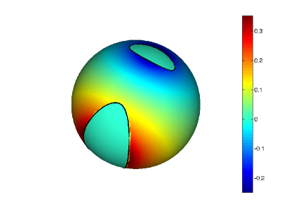
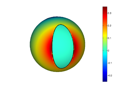
Figure 4: A numerical solution of the Yukawa-Beltrami equation with $k=4$ in a two-ply connected domain viewed from two different angles. The exact solution is the sum of two fundamental solutions, each one centered inside the regions bounded by $\Gamma$

Table 1: The number of GMRES iterations and the error at a collection of points sufficiently far from $\Gamma$.

$N$	# GMRES	Trapezoid Error	Alpert Error
32	9	6.67E-5	5.54E-6
64	9	7.84E-6	9.66E-10
128	9	9.86E-7	2.28E-11
256	9	1.24E-7	3.68E-11
512	9	1.59E-8	1.76E-10
1024	9	1.84E-9	1.20E-10

4.2 The effect of $k$

We consider the same two-ply connected geometry illustrated in Figure 4. We solve (30) for varying values of $k>1/2$ using Alpert’s quadrature rule with $N=32$. We report the condition number of the resulting linear system and the required number of GMRES iterations in Table 2. We see that for larger values of $k$, the conditioning of the linear system improves, and the number of GMRES iterations decreases. In Figure 5, we plot the eigenvalues of the linear system for $k=1$ and $k=64$. We see that for larger values of $k$, the eigenvalues cluster more strongly around $1/2$ resulting in a smaller number of GMRES iterations and a smaller condition number.

Table 2: The condition number of the linear system corresponding to a discretization of (30) and the number of GMRES iterations as a function of the parameter $k$.

$k$	Condition Number	# GMRES
0.51	4.22E1	14
1	1.22E1	13
2	4.50E0	11
4	2.17E0	9
8	1.45E0	8
16	1.24E0	7
32	1.13E0	6
64	1.07E0	6

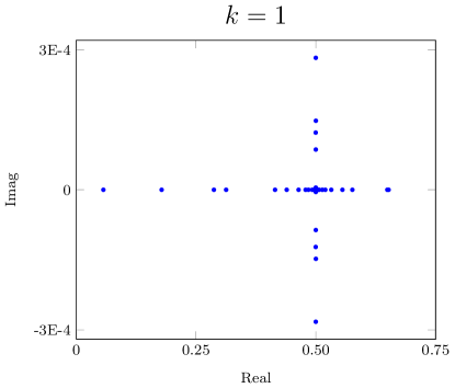
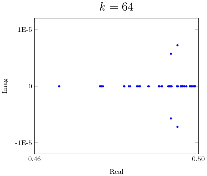
Figure 5: The eigenvalues of a discretization of (30) for $k=1$ (left) and $k=64$ (right)

4.3 The effect of the geometry’s curvature

We let $\Omega$ be exterior of an ellipse with a varying aspect ratio of its major and minor axis. The boundary $\Gamma$ is discretized with $N=512$ points and is parameterized by $x(\alpha)=a\cos(\alpha)$, $y(\alpha)=b\sin(\alpha)$, and $z(\alpha)=\sqrt{1-x^{2}(\alpha)-y^{2}(\alpha)}$, where $a=0.8$ and $b$ is varied in Table 3. We see that the curvature does have an effect on the condition number of the corresponding linear system as well as on the required number of GMRES iterations.

Table 3: The condition number of the linear system corresponding to (30) and the number of required GMRES iterations with respect to the ratio $a/b$.

$\frac{a}{b}$	Condition Number	# GMRES
1	1.11E0	2
2	1.51E0	6
4	2.88E0	8
8	5.95E0	11
16	1.23E1	19
32	2.52E1	35
64	4.72E1	54
128	1.51E2	83
256	1.43E3	227

4.4 A complex domain

We take a 36-ply connected domain and set the boundary condition to be a constant value of one everywhere. We set the parameter of the PDE to be $k=4$ and each boundary is discretized with $N=32$ points. The resulting linear system has 1152 unknowns, a condition number of $7.58$, and GMRES requires 25 iterations to reach the desired tolerance of 11 digits. A plot of the solution is in Figure 6.

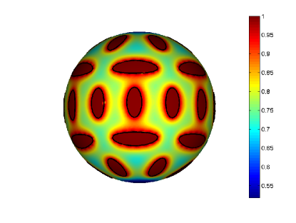
Figure 6: The numerical solution of the Yukawa-Beltrami equation with $k=4$ in a 36-ply connected domain. The Dirichlet boundary condition is equal to one on each of the boundaries (black curves)

5 Conclusions and Discussion

We have presented an integral equation strategy to solve the Dirichlet boundary value problem for the Yukawa-Beltrami equation on a multiply-connected, sub-manifold of the unit sphere. The integral equation formulation is based on a representation of a particularly useful form of a parametrix for the Yukawa-Beltrami operator involving conical functions. Using a double-layer ansatz based on this parametrix, a well-conditioned Fredholm equation of the second kind arises. Numerical experiments confirm the analytic properties of this integral equation and by selecting appropriate quadrature rules, we are able to compute highly accurate solutions. This integral equation formulation is amenable to acceleration either by a fast multipole method or a fast direct solver; this is future work.

The Yukawa-Beltrami equation arises when a temporal discretization is applied to the heat equation. However, the solution of (1) requires solving both a forced and a homogeneous problem. While the present work is designed to solve the homogeneous problem, future work involves using volume potentials to form solutions to the forced problem, as is done in rothe:heat for the heat equation in the plane.

Other future work includes extending the presented methods to other elliptic PDEs such as the Helmholtz or Stokes equations, and also to other two-dimensional manifolds. This will potentially create a new class of methods for solving problems involving scattering or fluid mechanics on the surface of smooth manifolds.

- (1) Alpert, B.K.: Hybrid Gauss-Trapezoidal Quadrature Rules. SIAM Journal on Scientific Computing 20, 1551–1584 (1999)
- (2) Bertalmio, M., Cheng, L.T., Osher, S., Sapiro, G.: Variational Problems and Partial Differential Equations on Implicit Surfaces. Journal of Computational Physics 174(2), 759–780 (2001). DOI 10.1006/jcph.2001.6937. URL http://www.sciencedirect.com/science/article/pii/S0021999101969372
- (3) Chaplain, M., Ganesh, M., Graham, I.: Spatio-temporal Pattern Formation on Spherical Surfaces: Numerical Simulation and Application to Solid Tumour Growth. J. Math. Biology 42, 387–423 (2001)
- (4) Floater, M.S., Hormann, K.: Surface Parameterization: a Tutorial and Survey. In: N.A. Dodgson, M.S. Floater, M.A. Sabin (eds.) Advances in Multiresolution for Geometric Modelling, Mathematics and Visualization, pp. 157–186. Springer Berlin Heidelberg (2005). DOI 10.1007/3-540-26808-1_9. URL http://dx.doi.org/10.1007/3-540-26808-1_9
- (5) Gatica, G.N., Hsiao, G.C., Sayas, F.J.: Relaxing the hypotheses of Bielak-MacCamy’s BEM-FEM coupling. Numer. Math. 120(3), 465–487 (2012). DOI 10.1007/s00211-011-0414-z. URL http://dx.doi.org/10.1007/s00211-011-0414-z
- (6) Gemmrich, S., Nigam, N., Steinbach, O.: Boundary Integral Equations for the Laplace-Beltrami Operator. Mathematics and Computation, a Contemporary View 3, 21–37 (2008)
- (7) Hackbusch, W.: Integral equations, International Series of Numerical Mathematics, vol. 120. Birkhäuser Verlag, Basel (1995). DOI 10.1007/978-3-0348-9215-5. URL http://dx.doi.org/10.1007/978-3-0348-9215-5. Theory and numerical treatment, Translated and revised by the author from the 1989 German original
- (8) Kropinski, M., Quaife, B.: Fast integral equation methods for the modified Helmholtz equation. Journal of Computational Physics 230, 425–434 (2011)
- (9) Kropinski, M.C.A., Nigam, N.: Fast integral equation methods of the Laplace-Beltrami equation on the sphere. Advances in Computational Mathematics 40, 577–596 (2014)
- (10) Kropinski, M.C.A., Quaife, B.: Fast Integral Equation Methods for Rothe’s Method Applied to the Isotropic Heat Equation. Comput. Math. Appl. 61(9), 2436–2446 (2011)
- (11) Lebedev, N.N.: Special functions and their applications. Dover Publications Inc., New York (1972). Revised edition, translated from the Russian and edited by Richard A. Silverman, Unabridged and corrected republication
- (12) Lindblom, L., Szilágyi, B.: Solving partial differential equations numerically on manifolds with arbitrary spatial topologies. Journal of Computational Physics 243, 151–175 (2013)
- (13) Myers, T., Charpin, J.: A mathematical model for atmospheric ice accretion and water flow on a cold surface. International Journal of Heat and Mass Transfer 47(25), 5483–5500 (2004). DOI 10.1016/j.ijheatmasstransfer.2004.06.037. URL http://www.sciencedirect.com/science/article/pii/S0017931004002807
- (14) Olver, F.W.J., Lozier, D.W., Boisvert, R.F., Clark, C.W. (eds.): NIST handbook of mathematical functions. U.S. Department of Commerce National Institute of Standards and Technology, Washington, DC (2010). With 1 CD-ROM (Windows, Macintosh and UNIX)
- (15) Quaife, B.: Fast Integral Equation Methods for the Modified Helmholtz Equation. Ph.D. thesis, Simon Fraser University (2011)
- (16) Ruuth, S.J., Merriman, B.: A simple embedding method for solving partial differential equations on surfaces. Journal of Computational Physics 227(3), 1943–1961 (2008). DOI 10.1016/j.jcp.2007.10.009. URL http://www.sciencedirect.com/science/article/pii/S002199910700441X
- (17) Witkin, A., Kass, M.: Reaction-diffusion textures. SIGGRAPH Comput. Graph. 25(4), 299–308 (1991). DOI 10.1145/127719.122750. URL http://doi.acm.org/10.1145/127719.122750