Efficient numerical solution of the time fractional diffusion equation by mapping from its Brownian counterpart

Abstract

The solution of a Caputo time fractional diffusion equation of order $0<\alpha<1$ is expressed in terms of the solution of a corresponding integer order diffusion equation. We demonstrate a linear time mapping between these solutions that allows for accelerated computation of the solution of the fractional order problem. In the context of an $N$-point finite difference time discretisation, the mapping allows for an improvement in time computational complexity from $O\left(N^{2}\right)$ to $O\left(N^{\alpha}\right)$, given a precomputation of $O\left(N^{1+\alpha}\ln N\right)$. The mapping is applied successfully to the least squares fitting of a fractional advection-diffusion model for the current in a time-of-flight experiment, resulting in a computational speed up in the range of one to three orders of magnitude for realistic problem sizes.

I Introduction

Derivatives of non-integer order have been particularly successful in describing a variety of complex processes with memory effects. These include applications in statistical finance (Scalas et al., 2000), economic modelling (Škovránek et al., 2012), image processing (Janev et al., 2011), quantum systems (Wu et al., 2014) and kinetics (Sokolov et al., 2002; Pagnini, 2014; Philippa et al., 2014, 2011; Sibatov and Uchaikin, 2007; Sagi et al., 2012; Toledo-Hernandez et al., 2014). This paper will focus on the numerical solution of a fractional kinetics description of anomalous diffusion. Unlike normal diffusion, whose mean squared displacement grows linearly with time, the anomalous diffusion considered here is characterised by a mean squared displacement that grows sublinearly according to a power law of the form $t^{\alpha}$ with $0<\alpha<1$ (Metzler and Nonnenmacher, 2002; Sokolov and Klafter, 2005; Sagi et al., 2012; Metzler et al., 1999; Metzler and Klafter, 2000). A number of stochastic approaches are capable of describing this kind of anomalous diffusion (Metzler et al., 1999; Metzler and Klafter, 2000; Klafter et al., 1987; Montroll and Weiss, 1965; Angstmann et al., 2014; Hilfer and Anton, 1995; Srokowski, 2014). For example, Scher and Montroll (Scher and Montroll, 1975) used a continuous time random walk (CTRW) model to describe the anomalous transport of charge carriers in disordered semiconductors. In this case, anomalous behaviour arises due to the localised trapping of charge carriers. To describe this trapping, a CTRW was chosen that sampled from a distribution of trapping times of the power law form $w\left(t\right)\sim t^{-\left(1+\alpha\right)}$. Here, $\alpha$ describes the severity of the trapping, with smaller values of $\alpha$ corresponding to increasingly severe traps. In disordered semiconductors, $\alpha$ arises physically from the energetic width of the density of localised states (Philippa et al., 2014; Sibatov and Uchaikin, 2007; Bisquert, 2003). It has been rigorously shown (Barkai et al., 2000; Metzler and Klafter, 2000, 2004) that a CTRW of this form can be described by a diffusion equation with a time derivative of fractional order $\alpha$. In this paper, we are concerned with the numerical solution of a Caputo fractional advection-diffusion model for the current in a time-of-flight experiment for a disordered semiconductor (Philippa et al., 2011; Uchaikin and Sibatov, 2008; Sibatov and Uchaikin, 2007; Sandev et al., 2011; Mainardi, 1996)

$${}_{0}^{\mathrm{C}}\mathcal{D}_{t}^{\alpha}u\left(t,x\right)=D_{\mathrm{L}}\frac{\partial^{2}}{\partial x^{2}}u\left(t,x\right)-W\frac{\partial}{\partial x}u\left(t,x\right),$$ (1)

where $W$ is a generalised drift velocity, $D_{\mathrm{L}}$ is a generalised diffusion coefficient and the operator for Caputo fractional differentiation of order $0<\alpha<1$ is defined in terms of the convolution integral (Caputo, 1967)

$${}_{0}^{\mathrm{C}}\mathcal{D}_{t}^{\alpha}f\left(t\right)\equiv\frac{1}{\Gamma\left(1-\alpha\right)}\int_{0}^{t}\mathrm{d}\tau\left(t-\tau\right)^{-\alpha}f^{\prime}\left(\tau\right).$$ (2)

Note that the normal advection-diffusion equation can be recovered in the relevant limit of no trapping

$$\lim_{\alpha\rightarrow 1}{}_{0}^{\mathrm{C}}\mathcal{D}_{t}^{\alpha}u\left(t,x\right)=\frac{\partial}{\partial t}u\left(t,x\right).$$ (3)

Numerous methods exist (Gao and Sun, 2011; Gao et al., 2014; Zhang et al., 2014; Yang et al., 2014; Bhrawy et al., 2014; Fu et al., 2013; Wu, 2010) for finding the numerical solution of fractional differential equations of the form of Eq. (1). Many of these are direct analogues to approaches that are also applicable to integer order differential equations. This is to be expected with the definition of fractional differentiation (2) defined in terms of both differentiation and integration. Unfortunately, when solving fractional differential equations numerically there is an increase (Podlubny, 1998) in time computational complexity over that encountered when solving differential equations of integer order. This is due to the global nature of fractional differentiation and, as in the case of anomalous diffusion, can be interpreted as a result of the system having memory. Consequently, any numerical algorithm that computes the solution at a present point in time requires the entire solution history to do so. In the context of an $N$-point finite difference time discretisation, this causes a time computational complexity increase from $O\left(N\right)$ to $O\left(N^{2}\right)$ (Ford and Simpson, 2001).

A number of approaches have been proposed to accelerate the computation of the numerical solution of fractional differential equations (Podlubny, 1998; Ford and Simpson, 2001; Fukunaga and Shimizu, 2011; Diethelm, 2011; Gong et al., 2014). As this added computational complexity stems from the memory inherent to the system, many of these approaches involve restricting this memory in some way. Podlubny (Podlubny, 1998) considered this approach by introducing the fixed memory principle, which amounts to truncating the convolution integral in the definition of fractional differentiation (2). In effect, this restricts the memory of the system to a fixed interval of time into the past, subsequently allowing for the solution to be found numerically in $O\left(N\right)$ in exchange for some loss in solution accuracy. Unfortunately, the only way to guarantee the accuracy of a numerical method used in conjunction with the fixed memory principle is to choose a fixed interval of time that encompasses the entire history of the solution, returning the computational complexity to $O\left(N^{2}\right)$. Ford and Simpson (Ford and Simpson, 2001) demonstrated exactly this and, as an alternative, introduced the logarithmic memory principle, which samples from the solution history in a logarithmic fashion, allowing for the solution to be found in $O\left(N\ln N\right)$ without compromise in solution accuracy. Finally, a number of parallel computing algorithms have also been introduced (Diethelm, 2011; Gong et al., 2014). These approaches are viable ways for accelerating the computation of the solution although, as they often involve splitting the problem into smaller problems of the same computational complexity, they are ultimately still of $O\left(N^{2}\right)$.

In Section II of the current study, we show that the solution to the fractional advection-diffusion equation (1) can be related to the solution of the normal advection-diffusion equation through a linear mapping in time. This mapping relationship, which takes the form of a matrix multiplication, provides an approach for the numerical acceleration of the fractional solution. In Section III, an algorithm for the computation of the matrix that defines the linear mapping is presented that utilises the fast Fourier transform. Additionally, we show that many elements of this matrix may contribute negligibly to the solution and so can be neglected, subsequently allowing for even further acceleration. In Section IV, we demonstrate the accuracy of this mapping approach by benchmarking the numerical solution of a fractional relaxation equation against its exact analytic solution. In Section V, this mapping is applied successfully to accelerate the fitting of Eq. (1) to experimental data for a time-of-flight experiment. Finally, in Section VI, we present conclusions and briefly list possible applications of our approach to various generalisations of the considered fractional-order problem.

II Mapping between normal and fractional diffusion

In this section, we will explore accelerating the numerical solution of the fractional advection-diffusion equation (1) by relating it to the solution of the normal advection-diffusion equation

$$\frac{\partial}{\partial\tau}v\left(\tau,x\right)=D_{\mathrm{L}}\frac{\partial^{2}}{\partial x^{2}}v\left(\tau,x\right)-W\frac{\partial}{\partial x}v\left(\tau,x\right),$$ (4)

where $\tau$ has fractional units of time due to the presence of the generalised transport coefficients $D_{\mathrm{L}}$ and $W$. By enforcing both equivalent initial conditions and boundary conditions, we can relate these solutions using the known integral transform relationship (Bouchaud and Georges, 1990; Klafter and Zumofen, 1994; Saichev and Zaslavsky, 1997; Barkai and Silbey, 2000; Barkai, 2001)

$$u\left(t,x\right)=\int_{0}^{\infty}\mathrm{d}\tau A\left(\tau,t\right)v\left(\tau,x\right),$$ (5)

which also holds true for any other shared linear spatial operator in the considered advection-diffusion equations. Here, the kernel is defined

$$A\left(\tau,t\right)\equiv\mathcal{L}^{-1}\left\{s^{\alpha-1}\mathrm{e}^{-s^{\alpha}\tau}\right\}=\frac{\partial}{\partial\tau}\left[1-L_{\alpha}\left(\frac{t}{\sqrt[\alpha]{\tau}}\right)\right],$$ (6)

where $\mathcal{L}$ denotes the Laplace transform and $L_{\alpha}\left(t\right)$ is the one-sided Lévy distribution, which is expressible in terms of the one-sided Lévy density $l_{\alpha}\left(t\right)$ as

$$L_{\alpha}\left(t\right)\equiv\int_{0}^{t}\mathrm{d}\tau l_{\alpha}\left(\tau\right),\quad\mathcal{L}l_{\alpha}\left(t\right)\equiv\mathrm{e}^{-s^{\alpha}}.$$ (7)

This integral relationship is known as a subordination transformation, where $A\left(\tau,t\right)$ is the probability distribution function providing subordination of the random process governed by Eq. (1) on the physical time scale $t$ to that governed by Eq. (4) on the operational time scale $\tau$ (Bochner, 1955).

In order to determine the fractional order solution numerically, we wish to find a discrete analogue of this transform. We note that this relationship acts on time alone, independent of space. As such, in what follows, we shall consider the solutions $u\left(t,x\right)$ and $v\left(\tau,x\right)$ solely as functions of time and reintroduce spatial dependence at a later point. Performing separation of variables, we can instead consider the ordinary time differential equations

$${}_{0}^{\mathrm{C}}\mathcal{D}_{t}^{\alpha}u\left(t\right) = \lambda u\left(t\right),$$ (8)

$$\frac{\mathrm{d}}{\mathrm{d}\tau}v\left(\tau\right) = \lambda v\left(\tau\right).$$ (9)

where $\lambda$ is the separation constant or eigenvalue of the shared spatial operator. We will now perform a finite difference time discretisation of these ordinary differential equations. We will denote time steps by superscripts $u^{n}\equiv u\left(n\Delta t\right)$, where $\Delta t$ is the time step size and $n=0,\dots,N$ is the time step number with $N$ being the total number of time steps and $t\equiv N\Delta t$ being the present point in time. To numerically approximate the fractional time derivative we will make use of the L1 algorithm (Oldham and Spanier, 1974), which was introduced by Oldham and Spanier to approximate the Riemann-Liouville fractional derivative. This algorithm has since been applied by a number of authors (Gao and Sun, 2011; Gao et al., 2014; Lin and Xu, 2007; Murio, 2008; Zhao and Sun, 2011) to the Caputo fractional derivative, resulting in the approximation

$${}_{0}^{\mathrm{C}}\mathcal{D}_{t}^{\alpha}u\left(t\right)=\Delta t^{-\alpha}\sum_{n=1}^{N}w_{n}\left(u^{N-n+1}-u^{N-n}\right)+O\left(\Delta t\right),$$ (10)

where we have the quadrature weights defined

$$w_{n}\equiv\frac{n^{1-\alpha}-\left(n-1\right)^{1-\alpha}}{\Gamma\left(2-\alpha\right)}.$$ (11)

This discretisation of the Caputo fractional derivative includes the limiting case where $\alpha\rightarrow 1$ from which we can recover the Euler method

$$\frac{\mathrm{d}}{\mathrm{d}\tau}v\left(\tau\right)=\frac{v^{N}-v^{N-1}}{\Delta\tau}+O\left(\Delta\tau\right).$$ (12)

Applying these discretisations to the ordinary differential equations, respectively (8) and (9), yields the recurrence relationships for the finite difference solution approximations

$$\left(1-\lambda\frac{\Delta t^{\alpha}}{w_{1}}\right)u^{N} = \hat{w}_{N}u^{0}+\sum_{n=1}^{N-1}\left(\hat{w}_{n}-\hat{w}_{n+1}\right)u^{N-n},\quad\quad$$ (13)

$$\left(1-\lambda\Delta\tau\right)v^{N} = v^{N-1},$$ (14)

where we have introduced the normalised quadrature weights $\hat{w}_{n}\equiv w_{n}/w_{1}$. As expected, the fractional order solution at each time step depends on the entire solution history, while the integer order solution depends only the nearest prior point in the neighbourhood of the present. We can solve these recurrence relationships analytically for the present time step in terms of their respective initial conditions

$$u^{N} = \sum_{n=1}^{N}a_{Nn}\frac{u^{0}}{\left(1-\lambda\frac{\Delta t^{\alpha}}{w_{1}}\right)^{n}},$$ (15)

$$v^{N} = \frac{v^{0}}{\left(1-\lambda\Delta\tau\right)^{N}},$$ (16)

where $a_{Nn}$, which is yet to be determined, denotes the $n$-th weight in the weighted sum for the fractional order solution at the $N$-th time step. If we choose the integer order initial condition to coincide with the fractional one $v^{0}=u^{0}$ and also choose a time step size for the integer order case of $\Delta\tau=\Delta t^{\alpha}/w_{1}$ we can relate the solution to the fractional order problem directly to the solution of the integer order one as

$$u^{N}=\sum_{n=1}^{N}a_{Nn}v^{n}.$$ (17)

This is a discrete analogue of the continuous integral relationship (5) and so the weights $a_{Nn}$ can be interpreted as quadrature weights. We should expect this discrete analogue to coincide with the continuous relationship in the limit of many time steps $N$. Most generally, reintroducing spatial dependence and considering all time steps, we can write each weighted sum in the form of Eq. (17) using the matrix multiplication

$$\mathbf{U}=\mathbf{A}\mathbf{V},$$ (18)

where we have the matrix of quadrature weights

$$\mathbf{A}=\left[\begin{array}[]{ccc}a_{11}&0&0\\ \vdots&\ddots&0\\ a_{N1}&\cdots&a_{NN}\end{array}\right],$$ (19)

which allows for mapping from the integer order solution matrix

$$\mathbf{V}=\left[\begin{array}[]{ccc}\text{---}&\mathbf{v}^{1}&\text{---}\\ &\vdots\\ \text{---}&\mathbf{v}^{N}&\text{---}\end{array}\right],$$ (20)

to the fractional order solution matrix

$$\mathbf{U}=\left[\begin{array}[]{ccc}\text{---}&\mathbf{u}^{1}&\text{---}\\ &\vdots\\ \text{---}&\mathbf{u}^{N}&\text{---}\end{array}\right],$$ (21)

where the rows of these solution matrices correspond to the spatial solution at each time step for the same spatial points. As the mapping matrix $\mathbf{A}$ is lower triangular, determining the solution matrix $\mathbf{U}$ using this matrix multiplication is of $O\left(N^{2}\right)$. This is no better than directly applying Eq. (13) to find the solution recursively. Fortunately, this is only the case if we absolutely require the solution at every time step. Indeed, if we are content with the solution at a subset of the overall time steps, we can perform the matrix multiplication in Eq. (18) partially in $O\left(N\right)$. Consider, for example, stability limitations such as the Courant-Friedrichs-Lewy condition (Thomas, 1995) that arise in explicit finite difference schemes and may require time steps smaller than would otherwise be needed. In such a situation, we can solve the integer order problem with sufficiently small time steps (to satisfy the stability criterion), and then map it onto the fractional problem using sparser time steps. Of course, the usefulness of this approach also depends on the computational complexity in computing the required rows of the mapping matrix. Fortunately, as the solution mapping depends solely on the operator of fractional differentiation, the mapping matrix can be precomputed for a given value of $\alpha$ and used repeatedly. The precise computational complexity for computing the mapping matrix will be considered in Section III.

III The solution mapping matrix

In this section, we address the problem of efficiently computing and applying the mapping matrix $\mathbf{A}$, present in Eq. (18) for the numerical relationship between integer and fractional order solutions.

III.1 Computation of the mapping matrix $\mathbf{A}$ using the fast Fourier transform

Substitution of the fractional finite difference solution approximation (15) back into its recurrence relationship (13) allows us to express the elements of the mapping matrix $\mathbf{A}$ in the form of a generating function recurrence relationship

$$A_{n}\left(x\right)=\Omega\left(x\right)A_{n-1}\left(x\right),$$ (22)

where we have the generating function for the $n$-th column of the mapping matrix

$$A_{n}\left(x\right)\equiv\sum_{m\geq 1}a_{mn}x^{m},$$ (23)

with the first column given by the initial condition weights from Eq. (13)

$$A_{1}\left(x\right)\equiv\sum_{m\geq 1}\hat{w}_{m}x^{m},$$ (24)

and the generating function of past time step weights from Eq. (13)

$$\Omega\left(x\right)\equiv\sum_{m\geq 1}\left(\hat{w}_{m}-\hat{w}_{m+1}\right)x^{m}.$$ (25)

The Cauchy product (Apostol, 1997) allows us to write this generating function recurrence relationship explicitly using a discrete linear convolution

$$\left[\begin{array}[]{c}a_{nn}\\ \vdots\\ a_{Nn}\end{array}\right]=\left[\begin{array}[]{c}\hat{w}_{1}-\hat{w}_{2}\\ \vdots\\ \hat{w}_{N-n+1}-\hat{w}_{N-n+2}\end{array}\right]\ast\left[\begin{array}[]{c}a_{n-1,n-1}\\ \vdots\\ a_{N-1,n-1}\end{array}\right],$$ (26)

where the initial column vector is provided by its generating function $A_{1}\left(x\right)$

$$\left[\begin{array}[]{c}a_{11}\\ \vdots\\ a_{N1}\end{array}\right]=\left[\begin{array}[]{c}\hat{w}_{1}\\ \vdots\\ \hat{w}_{N}\end{array}\right].$$ (27)

This convolution representation can be implemented using the fast Fourier transform, allowing for the computation of an $N\times N$ mapping matrix in $O\left(N^{2}\ln N\right)$. Evidently, determining the mapping matrix alone is more computationally intensive than finding the finite difference solution recursively in only $O\left(N^{2}\right)$. Certain situations exist, however, where the mapping matrix may be precomputed and reused, allowing for computational benefit even with this larger computational complexity. One such situation is the focus of Section V, where the least squares fit of a fractional order model to experimental data is considered. Fortunately, as described in the following subsection, we are not limited to only these situations when it comes to useful application of this solution mapping.

III.2 Column truncation of the mapping matrix $\mathbf{A}$

The magnitude of the elements of the mapping matrix $\mathbf{A}$ is illustrated in Figure 1 for various values of the fractional differentiation order $\alpha$. It can be seen that, as $\alpha$ decreases, fewer elements are likely to contribute to the solution mapping. This suggests that we can truncate the mapping matrix at some point during its column-wise computation described by Eq. (26). Here, we will specifically consider truncating the weighted sum (17) corresponding to the solution at the last time step. As a simplification, we will take both integer and fractional order solutions to be constant and hence equal, allowing us to remove all solution dependence and focus on truncating the summation

 

 

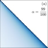
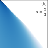
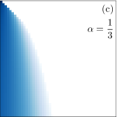
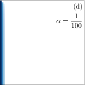
Figure 1: Illustration of the matrix $\mathbf{A}$ that maps from the solution of the normal diffusion equation (4) to the solution of the order $\alpha$ fractional diffusion equation (1). Each matrix is of size $50\times 50$ with elements that have been coloured according to their magnitude on a logarithmic scale. (a) As $\alpha\rightarrow 1$, the identity matrix is recovered, corresponding to the fractional and integer order solutions coinciding. (b-c) As $\alpha$ decreases, the matrix is dominated by elements with a lower column number, indicating that the early time solution to the integer order problem becomes increasingly significant. (d) As $\alpha\rightarrow 0$, the matrix approaches having only an initial column of ones, which corresponds to a time-invariant solution. This rapid decrease in element magnitude suggests the possibility of column-wise truncation of the mapping matrix, allowing for improved efficiency in both its computation and application, especially for small values of $\alpha$.

$$\sum_{n>0}a_{Nn}=1.$$ (28)

This expression can also be derived from the generating function representation (22) and is equivalent to stating that the rows of the mapping matrix sum to unity. Now, by introducing a truncation tolerance $0<\varepsilon<1$, which is proportional to the absolute error incurred by the truncation, we can define the number of columns in the truncated mapping matrix as the smallest integer $N_{\mathrm{trunc}}$ that satisfies

$$\sum_{n>N_{\mathrm{trunc}}}a_{Nn}\leq\varepsilon.$$ (29)

Evidently, to determine $N_{\mathrm{trunc}}$ using this inequality requires computation of matrix elements that will ultimately be truncated. Fortunately, using the row summation identity (28), we can restate this inequality using known matrix elements

$$\sum_{1\leq n\leq N_{\mathrm{trunc}}}a_{Nn}\geq 1-\varepsilon.$$ (30)

We can gain some insight into the asymptotic form of $N_{\mathrm{trunc}}$, and hence any computational benefit of this truncation, by considering the continuous analogue of this solution mapping, provided by Eq. (5). As before, by choosing an integer order solution that is constant, we find that

$$\int_{0}^{\infty}\mathrm{d}\tau A\left(\tau,t\right)=1,$$ (31)

which is evident from the Laplace space representation (6) of $A\left(\tau,t\right)$ as being the normalisation condition for an exponential distribution in $\tau$. By nondimensionalising in terms of the finite difference time step indices, that is taking $t=N\Delta t$ and $\tau=n\Delta t^{\alpha}/w_{1}$, we find the continuous analogue to the row summation identity (28)

$$\int_{0}^{\infty}\mathrm{d}na_{Nn}=1,\quad a_{Nn}\equiv\frac{\Delta t^{\alpha}}{w_{1}}A\left(\frac{n\Delta t^{\alpha}}{w_{1}},N\Delta t\right),$$ (32)

where both $n$ and $a_{Nn}$ are continuous here. Continuing with the analogy, we can now choose to truncate this integral at the point $n=N_{\mathrm{trunc}}$, resulting in the continuous analogue to truncation tolerance definition (29)

$$\varepsilon\equiv\int_{N_{\mathrm{trunc}}}^{\infty}\mathrm{d}na_{Nn}=L_{\alpha}\sqrt[\alpha]{\frac{w_{1}N^{\alpha}}{N_{\mathrm{trunc}}}},$$ (33)

where we have made use of the Lévy distribution representation (6) of the kernel $A\left(\tau,t\right)$. It is evident here that we can make this truncation tolerance an arbitrarily small constant that is independent of $N$ by choosing that $N_{\mathrm{trunc}}$ is directly proportional to $N^{\alpha}$. As the discrete truncation tolerance coincides with this continuous one in the limit of large $N$, we should expect to find the asymptotic behaviour $N_{\mathrm{trunc}}\sim N^{\alpha}$ for the continuous case. Indeed, Figure 2 shows precisely this as the size of the mapping matrix is increased for select values of $\alpha$. Therefore, when truncated, an $N\times N$ mapping matrix becomes of size $N\times O\left(N^{\alpha}\right)$, allowing for column-wise computation of it using the recurrence relationship (26) in only $O\left(N^{1+\alpha}\ln N\right)$. Similarly, we can now find the fractional order solution at particular instants in time in $O\left(N^{\alpha}\right)$. Finally, with this truncation, it should be noted that we are no longer required to precompute the mapping matrix in order to obtain a solution in a computational complexity better than $O\left(N^{2}\right)$.

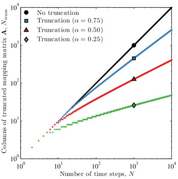
Figure 2: The number of columns in the mapping matrix $\mathbf{A}$, truncated according to the inequality (30) with a truncation tolerance of $\varepsilon=10^{-2}$. The gradient of each case approaches $\alpha$ as the number of time steps $N$ grow large, suggesting the asymptotic form $N_{\mathrm{trunc}}\sim N^{\alpha}$.

IV Benchmark of the truncated mapping

In this section, we will demonstrate the expected accuracy of the truncated mapping solution described in Section III relative to the direct finite difference solution provided either recursively or by the full mapping introduced in Section II. Specifically, we will consider the solution of the fractional relaxation equation (Metzler and Klafter, 2000)

$${}_{0}^{\mathrm{C}}\mathcal{D}_{t}^{\frac{1}{2}}u\left(t\right)=u\left(t\right),\quad u\left(0\right)=1,$$ (34)

which we chose because it has the exact analytic solution (Haubold et al., 2011)

$$u\left(t\right)=\mathrm{e}^{t}\left(1+\mathrm{erf}\sqrt{t}\right),$$ (35)

where $\mathrm{erf}\left(x\right)\equiv 2\pi^{-1/2}\int_{0}^{x}\mathrm{d}\xi\mathrm{e}^{-\xi^{2}}$ is the Gauss error function. Additionally, the finite difference solution here can be found recursively by simply taking Eqs. (13) and (14) with $\alpha=1/2$ and $\lambda=1$.

Figure 3 shows that the truncated mapping can be applied to find the solution to the fractional relaxation equation (34) to an accuracy comparable to the finite difference method, while still maintaining an improved computational complexity.

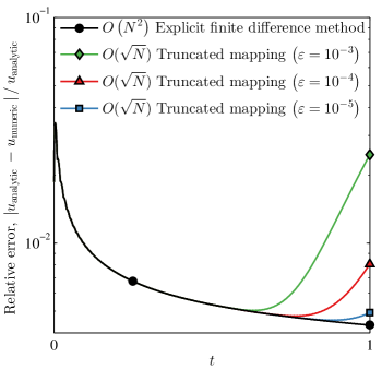
Figure 3: The error of an $N=100$ point finite difference solution of the fractional relaxation equation (34) relative to its analytic solution (35). The truncated solution mapping described in Section III is applied for decreasing values of the truncation tolerance $\varepsilon$. Note how the truncated mapping can be made to be arbitrarily accurate, while still retaining its computational complexity of $O\left(\sqrt{N}\right)$. The divergence in accuracy for late times stems from the truncation of more terms at later time steps. To perform this plot, a truncated mapping matrix $\mathbf{A}$ was precomputed in $O\left(N^{\frac{3}{2}}\ln N\right)$ and then truncated further as required.

V Application to the fitting of experimental data

Our approach is ideally suited to the acceleration of curve-fitting problems where the solution defining the curve must be found repeatedly and at relatively few points. In this section, we will demonstrate this by fitting a fractional-order model to experimental data for the current in a time-of-flight experiment for a disordered semiconductor. As stated in Section I, this can be described by the fractional advection-diffusion model (1). This model describes the charge carrier density in a thin sample held between two large plane-parallel boundaries with all spatial variation occurring normal to these boundaries. It will be assumed that the boundaries are perfectly absorbing, providing the Dirichlet boundary conditions

$$u\left(t,0\right)=0=u\left(t,d\right),$$ (36)

where $d$ is the thickness of the sample. We will choose the initial distribution of charge carriers to be governed by the Beer-Lambert law resulting in the exponential initial condition

$$u\left(0,x\right)\propto\mathrm{e}^{-ax},$$ (37)

where $a$ is the absorption coefficient of the sample. We can use the expression for the current in a time-of-flight experiment (Philippa et al., 2011)

$$I\left(t\right)\propto\frac{\partial}{\partial t}\int_{0}^{d}\left(\frac{x}{d}-1\right)u\left(t,x\right)\mathrm{d}x,$$ (38)

to find the current directly from the number density solution of Eq. (1). For spatial consideration, we will make use of the centred finite difference approximations

$$\frac{\partial}{\partial x}u\left(t,x\right) = \frac{u_{j+1}^{N}-u_{j-1}^{N}}{2\Delta x}+O\left(\Delta x^{2}\right),$$ (39)

$$\frac{\partial^{2}}{\partial x^{2}}u\left(t,x\right) = \frac{u_{j+1}^{N}-2u_{j}^{N}+u_{j-1}^{N}}{\Delta x^{2}}+O\left(\Delta x^{2}\right),$$ (40)

where $j=0,\dots,J$ is the spatial index, $J$ is the total number of spatial nodes and subscripts have been used to denote spatial indexing $u_{j}^{n}\equiv u\left(n\Delta t,j\Delta x\right)$. Hence, we can enforce the boundary conditions by setting $u_{0}^{n}=0=u_{J}^{n}$ for all $n=0,\dots,N$. Applying these spatial derivative approximations, in conjunction with Eq. (10) for approximating the Caputo fractional derivative, results in the recurrence relationship for the number density solution to Eq. (1)

$$\mathbf{C}\mathbf{u}^{N}=\hat{w}_{N}\mathbf{u}^{0}+\sum_{n=1}^{N-1}\left(\hat{w}_{n}-\hat{w}_{n+1}\right)\mathbf{u}^{N-n},$$ (41)

where we have the tridiagonal matrix

$$\mathbf{C}\equiv\left[\begin{array}[]{ccc}1-2r&r+s&0\\ r-s&1-2r&\ddots\\ 0&\ddots&\ddots\end{array}\right],\quad r\equiv-\frac{D_{\mathrm{L}}\Delta t^{\alpha}}{w_{1}\Delta x^{2}},\quad s\equiv\frac{W\Delta t^{\alpha}}{2w_{1}\Delta x}.$$ (42)

Figure 4 plots photocurrent data alongside the model (38) fitted using a trust-region-reflective non-linear least squares algorithm (Coleman and Li, 1994, 1996), as implemented in the lsqcurvefit function (lsq, 2014) located in MATLAB’s Curve Fitting Toolbox.

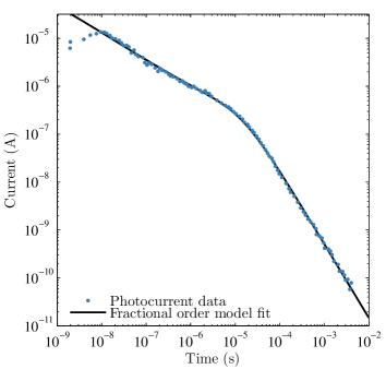
Figure 4: A least squares fit of the model (38) to the transient photocurrent in a sample of intrinsic hydrogenated amorphous silicon a-Si:H at 160K (adapted from Ref. (Scher et al., 1991)). To within a confidence interval of $95\%$, the fitting algorithm determined a severity of trapping of $\alpha=0.535\pm 2\%$, a generalised drift velocity of $Wd^{-1}t_{\mathrm{tr}}^{\alpha}=2.89\times 10^{-1}\pm 4\%$ and a generalised diffusion coefficient of $D_{\mathrm{L}}d^{-2}t_{\mathrm{tr}}^{\alpha}=6.07\times 10^{-3}\pm 21\%$, where the “transit time” separating the current regimes has been taken as $t_{\mathrm{tr}}\equiv 10^{-5}\mathrm{s}$.

To explore the computational benefits of applying the solution mapping described in Section II and its truncation described in Section III, we require the number density solution when $\alpha=1$, corresponding to normal transport. Proceeding as before, this time using Eq. (12) for the approximation of the first derivative, yields the recurrence relationship for the integer order solution $v\left(t,x\right)$

$$\mathbf{C}\mathbf{v}^{N}=\mathbf{v}^{N-1}.$$ (43)

As $\mathbf{C}$ is tridiagonal, we can step forward the fractional order solution recurrence relationship (41) in a time computational complexity of $O\left(J\right)$ (Press, 2007). As such, the total computational complexity to determine the fractional order solution in time and space becomes $O\left(N^{2}J\right)$. Similarly, by applying the solution mapping we have a computational complexity of $O\left(N^{2}J\ln N\right)$, which improves to $O\left(N^{1+\alpha}J\ln N\right)$ with truncation. The value of $\alpha$ present here can be estimated by noting the asymptotic form of the current in a time-of-flight experiment (Scher and Montroll, 1975)

$$I\left(t\right)\sim\begin{cases}t^{-\left(1-\alpha\right)},&\mathrm{early\,times},\\ t^{-\left(1+\alpha\right)},&\mathrm{late\,times},\end{cases}$$ (44)

which provides a criterion for recognising dispersive transport by noting that the sum of the slopes of the asymptotic regions of a current versus time plot on logarithmic axes is $-2$. In this particular case, we can use this criterion to bound the severity of trapping to within the interval $0.5<\alpha<0.55$.

Figure 5 plots the computation time for fitting the model (38) to the photocurrent data considered in Figure 4 for an increasing number of time steps. The observed fitting times do not increase monotonically with $N$. This is due to the nature of the fast Fourier transform (FFT) algorithm. The FFT is very sensitive to the prime factorisation of the input size. For example, the FFT is fastest when $N$ is a power of 2, and it is especially slow when $N$ is prime. Additional variations in fitting time may be due to the curve fitting algorithm and the number of iterations it requires to perform the fit.

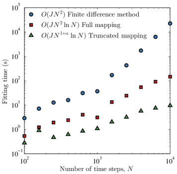
Figure 5: Comparison of computation time versus number of time steps for least squares fitting performed using the finite difference method (41), the accelerated solution mapping developed here (18) and the truncation thereof defined by Eq. (30). To maintain solution accuracy, the truncation tolerance $\varepsilon$ was chosen to decrease in proportion to $N$. It can be seen that the solution mapping without truncation is two orders of magnitude faster than the recursive approach for the largest problem size that was considered. With truncation, this improves to a three orders of magnitude speed up.

VI Concluding remarks and future work

Finite difference solutions to fractional differential equations are known to have a computation time that scales with the square of the number of time steps. This stems mathematically from the global nature of fractional differentiation, and physically can be interpreted as a consideration of memory effects. In this study, we have related the solution of the fractional diffusion equation (1) of order $0<\alpha<1$ to the solution of a the normal diffusion equation (4) using a linear mapping in time Eq. (18). We have found that, for an $N$-point finite difference time discretisation, we can use this mapping to improve upon the $O\left(N^{2}\right)$ time computational complexity of the finite difference method and determine the solution at any instant in time in $O\left(N^{\alpha}\right)$, given a precomputation of $O\left(N^{1+\alpha}\ln N\right)$. This representation is especially useful in situations where the solution must be found repeatedly, as then the relatively expensive precomputation only has to be performed once. We have presented one such situation in Section V where we have successfully applied this approach to fit the fractional advection-diffusion model (1) to experimental data for the current in a time-of-flight experiment. For this we achieved computational speed ups in the range of one to three orders of magnitude for the realistic problem sizes considered.

Although this work considered a fractional advection-diffusion model, the mapping approach described in this paper is applicable for any other linear spatial operator, including those of higher dimensions. With modifications, this solution mapping can be generalised to consider both the inclusion of a source term as well as higher order fractional derivatives for which $\alpha>1$.