Pairing sizes in attractively interacting Fermi gases with Spin-orbit Couplings

Abstract

Extensive research has been lavished on effects of spin-orbit couplings (SOC) in attractively interacting Fermi systems in both neutral cold atom systems and condensed matter systems. Recently, it was suggested that a SOC drives a new class of BCS to BEC crossover which is different than the conventional one without a SOC. Here, we explore what are the most relevant physical quantities to describe such a new BCS to BEC crossover and their experimental detections. We extend the concepts of the pairing length and “Cooper-pair size” in the absence of SOC to Fermi systems with SOC. We investigate the dependence of chemical potential, pairing length, “Cooper-pair size” on the SOC strength and the scattering length at $3d$ (the bound state energy at $2d$) for three attractively interacting Fermi gases with 3 dimensional (3d) Rashba, 3d Weyl and 2d Rashba SOC respectively. We show that only the pairing length can be used to characterize this new BCS to BEC crossover. Furthermore, it is the only length which can be directly measured by radio-frequency dissociation spectra type of experiments. We stress crucial differences among the pairing length, “Cooper-pair size ” and the two-body bound state size. Our results provide the fundamental and global picture of the new BCS to BEC crossover and its experimental detections in various cold atom and condensed matter systems.

I Introduction

Spin-orbit coupling (SOC) has played important roles in various condensed matter systems such as anomalous Hall effects ahe , non-centrosymmetric superconductors with lifted spin degeneracy socsemi and exciton superfluids in electron-hole semiconductor bilayers niu ; wu . Recently the investigation and control of spin-orbit coupling (SOC) have become subjects of intensive research after the discovery of the topological insulators Kane ; Zhang . For example, the SOC is a critical determining factor leading to a whole new class of electronic states kitpconf such as various spin-orbital ordered states, spin liquids, various topological phases, etc. The 1D SOC which is a linear combination of Rashba and Dresselhauss SOC has been successfully generated in several experimental groups for neutral atoms both in Bose and Fermi gas SOCexp ; SOCexp2 ; SOCexp3 ; gaugermp . Possible experimental constructions of 2D Rashba or Dresselhauss SOC and 3D Weyl SOC have also been proposed SOCtheo ; ZFXu . There are also extensive theoretical investigations on various important effects of SOC on attractively interacting twobody ; crossover ; zhai ; hu degenerate Fermi gases across BCS to BEC crossover. Collective excitations above the mean field states have also been calculated in collra2d ; collra3d ; colliso ; colliso2 . The collective modes and magnetic transitions in repulsively interacting Fermi gas were investigated replusive1 ; replusive2 . Recently, both staggered stagg and uniform uniform artificial magnetic fields have been generated in optical lattices. Scaling functions for various gauge-invariant and non-gauge invariant quantities across topological transitions driven by the SOC on an optical lattice have been derived topo . Especially, it was also stressed in topo that in contrast to condensed matter experiments where only gauge invariant quantities can be measured, both gauge invariant and non-gauge invariant quantities can be measured by experimentally generating various non-Abelian gauges corresponding to the same set of Wilson loops. The interplay among the SOC, interactions and lattice geometries leading to new quantum phase, excitation spectrum and quantum phase transitions has also been explored rh .

The BCS to BEC crossover is a long outstanding problem in both condensed matter superbook ; legg and cold atoms crossrmp . Conventional superconductors is well side the BCS limit, so mean field theory works well superbook ; legg . Due to its short coherence $\xi$, high temperature superconductors are near the BCS to BEC crossover, but still in the BCS side with well defined Fermi surface legg ; hightc , so quantum fluctuation effects are large. The BCS to BEC crossover of exciton superfluids in electron hole semiconductor bilayer can be tuned by the exciton density power ; squ ; excitoncorr ; exciton2 . The BCS to BEC crossovers of attractively interacting neutral fermions are tuned by sweeping across a Feshbach resonance crossrmp . The effects of SOC on the BCS to BEC crossover has been investigated by several groups twobody ; crossover ; zhai ; hu . Especially, the authors in crossover found that when the SOC strength is well beyond the value of the topological Lifshitz transition of the non-interacting Fermi surfaces replusive2 ; topo , the overlap between the two-body wavefunction twobody ; superbook and the “Cooper-pair wavefunction ” explain (see Sec. II-B for its definition) approaches to be 1. So they concluded that at a fixed scattering length at the BCS side (in the absence of SOC), the SOC drives a new BCS to BEC crossover which is in a different class than the one without a SOC driven by the exciton density power ; squ ; excitoncorr ; exciton2 or Feshbach resonance crossrmp . However, as to be shown in this paper, the “Cooper-pair wavefunction” is useful for illustration purposes only instead of being physical, so its overlap with the two-body wavefunction is not physical, can not be measured experimentally. In order to describe the new BCS to BEC crossover driven by the SOC strength, it is important to identify and compute the most relevant physical quantity to describe such a new BCS to BEC crossover and then address its experimental detections.

In this paper, we address this outstanding problem by investigating 3 SOC coupled Fermi gases: (1) a 3D Fermi gas with a Rashba SOC (2) a 3D Fermi gas with a isotropic Weyl SOC (3) a 2D Fermi gas with a Rashba SOC. We first extend the concepts of the pairing length associated with a many-body wavefunction superbook ; legg ; melo and “Cooper-pair size” explain associated with a “Cooper-pair wavefunction” in the absence of SOC to Fermi systems with a SOC. The three systems have different symmetries: the $[U(1)_{spin}\times U(1)_{orbit}]_{D}$ symmetry at 3d where the $D$ means the spontaneous rotation in spin and orbital space, the $[SU(2)_{spin}\times SO(3)_{orbit}]_{D}$ symmetry at 3d and the $[U(1)_{spin}\times U(1)_{orbit}]_{D}$ symmetry at 2d respectively. These symmetries determine the number of independent pairing lengths and Cooper-pair sizes to be 2, 1 and 1 respectively. We then study the dependence of chemical potential, pairing length, “Cooper-pair size” on the SOC strength $\lambda$ for three attractively interacting Fermi gases. We show that from the BCS side at $\lambda=0$, as the SOC strength increases, the chemical potential drops below the bottom of the single particle spectrum $\mu_{0}=-\frac{\lambda^{2}}{2m}$, so it can be used to characterize qualitatively the BCS to BEC crossovers driven by the SOC strength. The pairing length decreases monotonically and quickly below the inter-particle spacing, so can be used to characterize quantitatively the BCS to BEC crossovers. Furthermore, the pairing length can be directly measured by using radio-frequency dissociation spectra type of experiments mitdiss as soon as the 2d and 3d SOC can be realized experimentally. In sharp contrasts, the “Cooper-pair size” used in the previous work twobody ; crossover ; zhai shows non-monotonic behaviors, so it may not be used to characterize the BCS to BEC crossover even qualitatively. Furthermore, it is not an experimentally measurable quantity. Starting from the BEC side at $\lambda=0$, the effects of SOC are small, both the pairing length and the “Cooper-pair size” converge to the two-body bound state size twobody ; superbook . We conclude that the pairing length is a much more robust concept than the “Cooper pair size ”, it is also the only experimentally detectable physical quantity which can be used to describe the BCS to BEC crossover even quantitatively. We also discuss relations among the many-body BCS wavefunctions, the “Cooper-pair wavefunctions” and the two-body wavefunctions, therefore stress crucial differences among the pairing length, Cooper-pair size and the two body bound state size. The results provide a solid foundation for the fundamental physics of the new BCS to BEC crossover and its experimental detections. Our results should also shed considerable lights on condensed matter systems such as 2d exciton superfluids and 2d non-centrosymmetric superconductors.

The rest of the paper is organized as follows: In Sect. II, we first review the different definitions and concepts of pairing length and “Cooper pair size”, then extend their concepts to SOC system where the spin is not a conserved quantity. In Sect.III, for a 3d Rashba systems, we study how the chemical potential, the pairing length and the Cooper pair size change as the SOC strength increases, especially focus on their behaviors across the new BCS to BEC crossover driven by the SOC strength. To be complete, we also study how the the pairing length and the Cooper pair size change with the scattering lengths at fixed SOC strengths. We also discuss the crucial differences among the pairing length, Cooper-pair size and the two-body bound state size. In Sec.IV, we compute the same quantities on 3d Fermi gas with an isotropic Weyl SOC. In Sec.V, we perform similar calculations on 2d Fermi gas with Rashba SOC which needs a different regularization than the two 3d systems discussed in the previous two sections. In Sec.VI, we discuss the implications of the results achieved in the previous sections, especially in the Sec. V, on several condensed matter systems. We summarize the main results and discuss several exciting perspectives in Sec. VII.

II Extend paring length and Cooper pair size to SOC systems

We consider a homogeneous Fermi gas with an attractive contact potential:

$$H = \underset{\boldsymbol{p},\sigma=\uparrow,\downarrow}{\sum}c_{\boldsymbol{p}\sigma}^{\dagger}\left(\frac{\boldsymbol{p}^{2}}{2m}-\mu\right)c_{\boldsymbol{p}\sigma}+V_{soc}$$ (1)

$$+\frac{g}{V}\underset{\boldsymbol{p},\boldsymbol{q},\boldsymbol{s}}{\sum}c_{\frac{\boldsymbol{s}}{2}+\boldsymbol{p}\uparrow}^{\dagger}c_{\frac{\boldsymbol{s}}{2}-\boldsymbol{p}\downarrow}^{\dagger}c_{\frac{\boldsymbol{s}}{2}-\boldsymbol{q}\downarrow}c_{\frac{\boldsymbol{s}}{2}+\boldsymbol{q}\uparrow},$$

where $d=2,3$, and $V_{soc}$ is the spin-orbit coupling (SOC) term which can be Rashba or Dresselhauss type or 3d Weyl isotropic SOC.

It was known that the interaction $g$ need to be regularized differently in 2d and 3d. In 3d, the $g$ can be regularized by the s-wave scattering length $a_{s}$: $\frac{1}{g}=\frac{m}{4\pi\hbar^{2}a_{s}}-\frac{1}{V}\underset{\boldsymbol{p}}{\sum}\frac{1}{2\epsilon_{\boldsymbol{p}}}$ where $V$ is the volume of the system and $\epsilon_{\boldsymbol{p}}=\frac{\boldsymbol{p}^{2}}{2m}$ is the free particle dispersion. In 2d, the $g$ can be regularized by the two-body binding energy $\epsilon_{B}$: $\frac{1}{g}=-\frac{1}{V}\underset{\boldsymbol{p}}{\sum}\frac{1}{2\epsilon_{\boldsymbol{p}}+\epsilon_{B}}$.

By introducing the order parameter $\Delta=\frac{g}{V}\underset{\boldsymbol{p}}{\sum}\left\langle c_{-\boldsymbol{p}\downarrow}c_{\boldsymbol{p}\uparrow}\right\rangle$, one can reduce the interaction term to the mean-field form: $H_{int}^{MF}=\underset{\boldsymbol{p}}{\sum}\left(\Delta^{*}c_{-\boldsymbol{p}\downarrow}c_{\boldsymbol{p}\uparrow}+\Delta c_{\boldsymbol{p}\uparrow}^{\dagger}c_{-\boldsymbol{p}\downarrow}^{\dagger}\right)-\frac{V\left|\Delta\right|^{2}}{g}$. The chemical potential $\mu$ and the order parameter $\Delta$ can be determined by two self-consistent equations—the number equation: $n=\frac{1}{V}\underset{\boldsymbol{p,\sigma}}{\sum}\left\langle c_{\boldsymbol{p}\sigma}^{\dagger}c_{\boldsymbol{p}\sigma}\right\rangle_{MF}$ and the gap equation: $\Delta=\frac{g}{V}\underset{\boldsymbol{p}}{\sum}\left\langle c_{-\boldsymbol{p}\downarrow}c_{\boldsymbol{p}\uparrow}\right\rangle_{MF}$.

Without SOC, the pairing length has been calculated in Fermi gas across the whole BCS to BEC crossover tuned by Feshbach resonance in melo . Most importantly, it has been measured in MIT’s group lead by Ketterle using radio-frequency dissociation spectra throughout the whole BCS to BEC crossover in mitdiss . However, the effects of SOC on the pairing correlation lengths have never been studied so far. In this section, we first review the definition and concepts of the pairing length without SOC, then extend to the SOC case.

II.1 Pairing length

For a spin singlet superfluid without SOC, the fermion pair correlation functions are defined as:

$$\psi(\vec{r})=\frac{1}{n^{2}}\langle c^{\dagger}_{\uparrow}(\vec{r})c^{\dagger}_{\downarrow}(0)c_{\downarrow}(0)c_{\uparrow}(\vec{r})\rangle-\frac{1}{4},$$ (2)

where $n$ is the particle density and the average is taken with respect to the BCS ground state $|\Phi\rangle=|BCS\rangle$ (in second quantized form):

$$|\Phi\rangle = \Pi_{\vec{k}}(u_{\vec{k}}+v_{\vec{k}}c^{\dagger}_{\vec{k}\uparrow}c^{\dagger}_{-\vec{k}\downarrow})|0\rangle$$ (3)

$$= (\Pi_{\vec{k}}u_{\vec{k}})\Pi_{\vec{k}}(1+\frac{v_{\vec{k}}}{u_{\vec{k}}}c^{\dagger}_{\vec{k}\uparrow}c^{\dagger}_{-\vec{k}\downarrow})|0\rangle$$

$$= (\Pi_{\vec{k}}u_{\vec{k}})exp[\sum_{\vec{k}}\frac{v_{\vec{k}}}{u_{\vec{k}}}c^{\dagger}_{\vec{k}\uparrow}c^{\dagger}_{-\vec{k}\downarrow})]|0\rangle,$$

which obviously hosts in-definite number of electrons. Its first quantized form was discussed in superbook .

The pairing length is defined as melo ; mitdiss

$$\xi^{2}_{pair}=\frac{\int d\vec{r}\psi(\vec{r})r^{2}}{\int d\vec{r}\psi(\vec{r})}.$$ (4)

At the mean field level, Eqn.2 reduces to:

$$\psi(\vec{r})=\frac{1}{n^{2}}|\langle\Phi|c^{\dagger}_{\uparrow}(\vec{r})c^{\dagger}_{\downarrow}(0)|\Phi\rangle|^{2},$$ (5)

where $|\Phi\rangle=|BCS\rangle$.

Under the mean field approximation, Eqn.4 can be rewritten as mitdiss :

$$\xi^{2}_{pair}=\frac{\langle\psi_{\alpha\beta}|r^{2}|\psi_{\alpha\beta}\rangle}{\langle\psi_{\alpha\beta}|\psi_{\alpha\beta}\rangle},$$ (6)

where $\psi_{\alpha\beta}(\vec{r})=\langle\Phi|c^{\dagger}_{\alpha}(\vec{r})c^{\dagger}_{\beta}(0)|\Phi\rangle$ with $\alpha=\uparrow,\beta=\downarrow$.

The Fourier transform of Eqn.6 to $\vec{k}$ space leads to:

$$\xi^{2}_{pair}=\frac{\langle\psi_{\alpha\beta}|\nabla^{2}_{\vec{k}}|\psi_{\alpha\beta}\rangle}{\langle\psi_{\alpha\beta}|\psi_{\alpha\beta}\rangle},~{}~{}~{}~{}\alpha=\uparrow,\beta=\downarrow,$$ (7)

where $\psi_{\alpha\beta}(\vec{k})=\langle\Phi|c^{\dagger}_{\alpha}(\vec{k})c^{\dagger}_{\beta}(-\vec{k})|\Phi\rangle$ is the Fourier transform of $\psi_{\alpha\beta}(\vec{r})$ with $\alpha=\uparrow,\beta=\downarrow$. More straightforwardly, Eqn.6 in real space and Eqn.7 in momentum space are Fourier transform to each other.

For a BEC to BCS crossover without SOC, the only pairing is the singlet pairing so $\psi_{\uparrow\downarrow}(\vec{k})=\langle\Phi|c^{\dagger}_{\uparrow}(\vec{k})c^{\dagger}_{\downarrow}(-\vec{k})|\Phi\rangle=u_{\vec{k}}v_{\vec{k}}=\frac{\Delta_{0}}{2E_{\vec{k}}}$ which is given and shown in Fig.3 in melo .

It is important to point out that Eqn.2 and Eqn.4 hold in general, while Eqn.5 and 6 hold only at the mean field level. Only at the mean field level, one can “intuitively” interpret Eqn.5 and 6 as the expectation value of $r^{2}$ over the “pairing wavefunction” $\psi_{\alpha\beta}(\vec{r})=\langle\Phi|c^{\dagger}_{\alpha}(\vec{r})c^{\dagger}_{\beta}(0)|\Phi\rangle$ with $\alpha=\uparrow,\beta=\downarrow$. Although the concept of pairing length Eqn.4 hold in general, such a wavefunction interpretation breaks down beyond the mean field.

In the presence of SOC, due to the non-conservation of spins, one need to average over all the spin components to define the fermion pair correlation functions, so Eqn.2 should be replaced by

$$\psi(\vec{r})=\frac{1}{n^{2}}\sum_{\alpha,\beta}\langle c^{\dagger}_{\alpha}(\vec{r})c^{\dagger}_{\beta}(0)c_{\beta}(0)c_{\alpha}(\vec{r})\rangle-1,$$ (8)

where $n$ is the particle density. Eqn.4 remains.

At mean field level, following the steps to derive Eqns.5 and 6 leads to the pairing length in the presence of SOC:

$$\xi^{2}_{i}=\frac{\sum_{\vec{k},\alpha,\beta}\langle\psi_{\alpha\beta}|\partial^{2}_{k_{i}}|\psi_{\alpha\beta}\rangle}{\sum_{\vec{k},\alpha,\beta}\langle\psi_{\alpha\beta}|\psi_{\alpha\beta}\rangle},~{}~{}~{}~{}\alpha,\beta=\uparrow,\downarrow,$$ (9)

which could be measured by radio-frequency dissociation spectra used in the experiment mitdiss in the presence of SOC. After the spin sum, the orbital symmetry of the $U(1)_{orbit},O(3)_{orbit},U(1)_{orbit}$ of the three systems to be discussed in the following three sections will be recovered. However, one still need to distinguish the pairing correlation length within $xy$ plane and along $z$ direction $\xi^{2}_{xy}\neq\xi^{2}_{z}$ in the first and the third system.

II.2 “Cooper pair size”

In fact, one can also define the “Cooper-pair size” through the “Cooper pair wavefunction” superbook ; read . Removing the exponential in the normalized BCS wave function without SOC in Eqn.3 leads to the singlet “Cooper-pair wavefunction” in second quantized form:

$$|g_{cp}\rangle=\sum_{\vec{k}}\frac{v_{\vec{k}}}{u_{\vec{k}}}c^{\dagger}_{\vec{k}\uparrow}c^{\dagger}_{-\vec{k}\downarrow}|0\rangle,$$ (10)

which hosts only two paired electrons. It can be understood as the two electron components of the many-body wavefunction.

One can extract the “Cooper-pair wavefunction” in the real space in the first quantization:

$$g_{cp}(\vec{r})=g_{\uparrow\downarrow}(\vec{r})(|\uparrow\downarrow\rangle-|\downarrow\uparrow\rangle),~{}~{}g_{\uparrow\downarrow}(\vec{r})=\sum_{\vec{k}}e^{i\vec{k}\cdot\vec{r}}\frac{v_{\vec{k}}}{u_{\vec{k}}}.$$ (11)

It is necessary to point out that this “Cooper-pair wavefunction” is different than the original pairing problem of two electrons near a Fermi surface first achieved by Cooper by solving the Schrodinger equation superbook .

The “Cooper pair size” explain is defined by superbook ; read

$$l^{2}_{pair}=\frac{\int d\vec{r}|g_{\uparrow\downarrow}(\vec{r})|^{2}r^{2}}{\int d\vec{r}|g_{\uparrow\downarrow}(\vec{r})|^{2}}=\frac{\left\langle g_{cp}\right|r^{2}\left|g_{cp}\right\rangle}{\left\langle g_{cp}|g_{cp}\right\rangle}.$$ (12)

The Fourier transform of Eqn.12 to $\vec{k}$ space leads to:

$$l^{2}_{pair}=\frac{\langle g_{\alpha\beta}|\nabla^{2}_{\vec{k}}|g_{\alpha\beta}\rangle}{\langle g_{\alpha\beta}|g_{\alpha\beta}\rangle},~{}~{}~{}~{}\alpha=\uparrow,\beta=\downarrow,$$ (13)

where $g_{\uparrow\downarrow}(\vec{k})=\frac{v_{\vec{k}}}{u_{\vec{k}}}$ is the Fourier transform of $g_{\uparrow\downarrow}(\vec{r})$. This should be contrasted with $\psi_{\uparrow\downarrow}(\vec{k})=\langle\Phi|c^{\dagger}_{\uparrow}(\vec{k})c^{\dagger}_{\downarrow}(-\vec{k})|\Phi\rangle=u_{\vec{k}}v_{\vec{k}}=\frac{\Delta_{0}}{2E_{\vec{k}}}$ used in Eqn.7.

It is important to point out that Eqn.3,11,12,13 hold only in mean field level. Only at the mean field level, one can “intuitively” interpret Eqn.12 and 13 as the expectation value of $r^{2}$ over the “Cooper-pair wavefunction” Eqn.11. However, the concept of Cooper-pair size Eqn.13 breaks down beyond the mean field theory.

In the presence of SOC, after writing the mean field ground state in the form $|BCS\rangle_{SOC}\propto exp[\sum_{\vec{k}}g_{\alpha\beta}(\vec{k})c^{\dagger}_{\vec{k}\alpha}c^{\dagger}_{-\vec{k}\beta}]|0\rangle$, then one can extract the Cooper pair size superbook ; read as

$$l^{2}_{i}=\frac{\sum_{\vec{k},\alpha,\beta}\langle g_{\alpha\beta}|\partial^{2}_{k_{i}}|g_{\alpha\beta}\rangle}{\sum_{\vec{k},\alpha,\beta}\langle g_{\alpha\beta}|g_{\alpha\beta}\rangle},~{}~{}~{}~{}\alpha,\beta=\uparrow,\downarrow,$$ (14)

where the average over all the spin components is performed. Note that $g_{\alpha\beta}(\vec{k})$ is very much different than $\phi_{\alpha\beta}(\vec{k})$, so we may expect quite different behaviors from the two lengths. These will be explicitly demonstrated in the following sections. It is the pairing length which is measured in the MIT experiment mitdiss .

In the following, we apply the formalism to the 3d Rashba SOC, 3d Weyl SOC and 2d Rashba SOC systems.

III 3D Fermi gas with a Rashba SOC

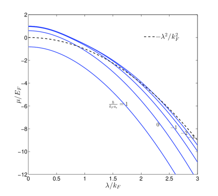
Figure 1: The chemical potential $\mu$ versus $\lambda$ in a 3D Rashba SOC for different scattering lengths. The dashed line is the bottom of the single particle spectrum $\mu_{0}=-\frac{\lambda^{2}}{2m}$. Starting from the BCS side at $\lambda=0$, as $\lambda$ increases, the $\mu$ drops below $\mu_{0}$. This fact indicates that the system evolves into the BEC state.

The 3d Rashba SOC can be written as

$$V_{3d-ra}=\frac{\lambda}{m}\underset{\boldsymbol{p}}{\sum}p_{\perp}\left[e^{-i\varphi_{\boldsymbol{p}}}c_{\boldsymbol{p}\uparrow}^{\dagger}c_{\boldsymbol{p}\downarrow}+e^{i\varphi_{\boldsymbol{p}}}c_{\boldsymbol{p}\downarrow}^{\dagger}c_{\boldsymbol{p}\uparrow}\right],$$ (15)

where $\lambda$ is the SOC strength, $p_{\perp}=\sqrt{p_{x}^{2}+p_{y}^{2}}$ and $\varphi_{\boldsymbol{p}}=Arg\left(p_{x}+ip_{y}\right)$. This model has been studied by previous works zhai ; hu with different focuses. The single particle part $H_{0}$ in the Hamiltonian Eq. 1 can be diagonalized in the helicity base as

$$H_{0}=\underset{\boldsymbol{p}}{\sum}\left(\xi_{\boldsymbol{p}+}h_{\boldsymbol{p}+}^{\dagger}h_{\boldsymbol{p}+}+\xi_{\boldsymbol{p}-}h_{\boldsymbol{p}-}^{\dagger}h_{\boldsymbol{p}-}\right),$$ (16)

where $\xi_{\boldsymbol{p}\pm}=\frac{p^{2}}{2m}\pm\frac{\lambda p_{\perp}}{m}-\mu$ and the two helicity operators are:

$$h_{\boldsymbol{p}+} = \left[c_{\boldsymbol{p}\uparrow}+e^{-i\varphi_{\boldsymbol{p}}}c_{\boldsymbol{p}\downarrow}\right]/\sqrt{2},$$

$$h_{\boldsymbol{p}-} = \left[e^{i\varphi_{\boldsymbol{p}}}c_{\boldsymbol{p}\uparrow}-c_{\boldsymbol{p}\downarrow}\right]/\sqrt{2}.$$ (17)

.

In the helicity base, the mean-field interaction can be rewritten as $H_{int}^{MF}=-\frac{1}{2}\underset{\boldsymbol{p}}{\sum}\left(\Delta_{0}e^{-i\varphi_{\boldsymbol{p}}}h_{\boldsymbol{p}+}^{\dagger}h_{\boldsymbol{-p}+}^{\dagger}+\Delta_{0}e^{i\varphi_{\boldsymbol{p}}}h_{\boldsymbol{p}-}^{\dagger}h_{\boldsymbol{-p}-}^{\dagger}+h.c.\right)-\frac{V\left|\Delta\right|^{2}}{g}$. The total Hamiltonian $H=H_{0}+H_{int}^{MF}$ can be diagonalized by a Bogoliubov transformation:

$$H = \underset{\boldsymbol{p}}{\sum}\left(E_{\boldsymbol{p}+}\alpha_{\boldsymbol{p}+}^{\dagger}\alpha_{\boldsymbol{p}+}+E_{\boldsymbol{p}-}\alpha_{\boldsymbol{p}-}^{\dagger}\alpha_{\boldsymbol{p}-}\right)$$ (18)

$$- \underset{\boldsymbol{p}}{\sum}\frac{E_{\boldsymbol{p}+}+E_{\boldsymbol{p}-}}{2}-\frac{V\left|\Delta_{0}\right|^{2}}{g},$$

where the quasiparticle excitation energy $E_{\boldsymbol{p}\pm}=\sqrt{\xi_{\boldsymbol{p}\pm}^{2}+\left|\Delta_{0}\right|^{2}}$, and the quasi-particle operators:

$$\alpha_{\boldsymbol{p}+} = \sqrt{\frac{E_{\boldsymbol{p}+}+\xi_{\boldsymbol{p}+}}{2E_{\boldsymbol{p}+}}}e^{i\varphi_{\boldsymbol{p}}}h_{\boldsymbol{p}+}-\sqrt{\frac{E_{\boldsymbol{p}+}-\xi_{\boldsymbol{p}+}}{2E_{\boldsymbol{p}+}}}h_{-\boldsymbol{p}+}^{\dagger},$$

$$\alpha_{\boldsymbol{p}-} = \sqrt{\frac{E_{\boldsymbol{p}-}+\xi_{\boldsymbol{p}-}}{2E_{\boldsymbol{p}-}}}e^{-i\varphi_{\boldsymbol{p}}}h_{\boldsymbol{p}-}-\sqrt{\frac{E_{\boldsymbol{p}-}-\xi_{\boldsymbol{p}-}}{2E_{\boldsymbol{p}-}}}h_{-\boldsymbol{p}-}^{\dagger},$$ (19)

where all anticommutation relations hold ($\left\{\alpha_{\boldsymbol{p}+},\alpha_{\boldsymbol{p}+}^{\dagger}\right\}=1$, $\left\{\alpha_{\boldsymbol{p}+},\alpha_{\boldsymbol{p}-}^{\dagger}\right\}=0$, and so on).

At zero temperature, the two self-consistent equations become

$$n = \frac{1}{V}\underset{\boldsymbol{p}}{\sum}\left[1-\frac{\xi_{\boldsymbol{p}+}}{2E_{p+}}-\frac{\xi_{\boldsymbol{p}-}}{2E_{p-}}\right],$$

$$\frac{1}{g} = -\frac{1}{4V}\underset{\boldsymbol{p}}{\sum}\left[\frac{1}{E_{p+}}+\frac{1}{E_{p-}}\right],$$ (20)

where, as said in the Sec.II, the interaction strength $g$ can be regularized by the s-wave scattering length $a_{s}$: $\frac{1}{g}=\frac{m}{4\pi\hbar^{2}a_{s}}-\frac{1}{V}\underset{\boldsymbol{p}}{\sum}\frac{1}{2\epsilon_{\boldsymbol{p}}}$. In the rest of the section, we will determine the chemical potential $\mu$, the paring length $\xi_{i}$ in Eqn.9, the Cooper pair size $l_{i}$ in Eqn.14. Finally we will compare our many body results with the corresponding two-body results twobody .

III.1 Chemical potential across BCS to BEC crossover

One can find the chemical potential $\mu$ by solving Eqn.20. It is shown in Fig.1. As a contrast, the minimum of the single-particle excitation energy $\mu_{0}=\underset{\boldsymbol{p}}{\text{Min}}\{\frac{p^{2}}{2m}-\frac{\lambda p_{\perp}}{m}\}=-\frac{\lambda^{2}}{2m}$ is also plotted in Fig.1. We can qualitatively assign the region with $\mu>\mu_{0}$ as the BCS region and $\mu<\mu_{0}$ as the BEC region. As shown in Fig.1, starting from the BCS side at $\lambda=0$, as $\lambda$ increases, the $\mu$ drops below $\mu_{0}$. Therefore, we conclude that Rashba SOC can drive a crossover from BCS to BEC as first pointed out in crossover .

III.2 Pairing length across BCS to BEC crossover

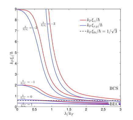
Figure 2: The pairing length defined in Eqn.9 along $x$ direction (red lines) ( $\xi_{x}=\xi_{y}$) and along the $z$ (blue lines) direction as a functions of 3d Rashba SOC strength $\lambda$. The dashed line is a guidance line where $k_{F}\xi_{0}=\hbar$ ($k_{F}\xi_{0i}=\hbar/\sqrt{3}$ for each component). Starting from the BCS side at $\lambda=0$, it decreases monotonically and quickly below the reference line, so describe precisely the new BCS to BEC crossover driven by the SOC strength. Starting from the BEC side at $\lambda=0$, the effects of SOC are small.

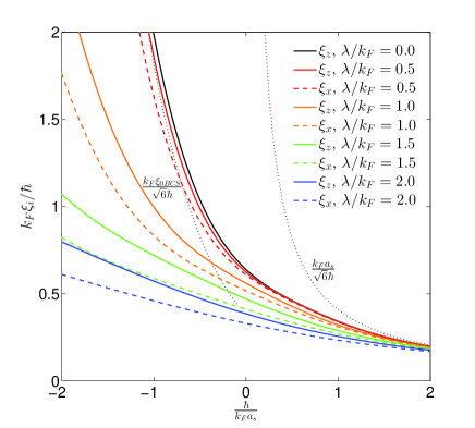
Figure 3: The pairing lengths $\xi_{z}>\xi_{x}=\xi_{y}$ at a fixed 3d Rashba SOC strength versus the scattering length. Different colors stand for different SOC strengths. Solid (dashed) lines stand for $\xi_{z}$ ($\xi_{x}=\xi_{y}$). The dark dotted line on the left (right) is its BCS (BEC) limit $\frac{1}{\sqrt{6}}k_{F}\xi_{0BCS}=\frac{1}{8\sqrt{6}e^{2}}e^{-\frac{\pi\hbar}{2k_{F}a_{s}}}$ ($\frac{k_{F}a_{s}}{\sqrt{6}}$) at $\lambda=0$. On the BCS side, the SOC effects are dramatic, but on the BEC side, the SOC effects are small, all curves converge to the right dotted line $\frac{k_{F}a_{s}}{\sqrt{6}}$ from below.

The BCS ground state can be written as:

$$\left|BCS\right\rangle=\underset{\boldsymbol{p}}{\prod}^{\prime}\alpha_{\boldsymbol{p}+}\alpha_{-\boldsymbol{p}+}\alpha_{\boldsymbol{p}-}\alpha_{-\boldsymbol{p}-}\left|0\right\rangle~{}~{}~{}~{}~{}~{}~{}~{}~{}~{}~{}~{}~{}~{}~{}~{}$$

$$\propto\exp\underset{\boldsymbol{p}}{\sum}^{\prime}\left[w_{\boldsymbol{p}+}e^{-i\varphi_{\boldsymbol{p}}}h_{\boldsymbol{p}+}^{\dagger}h_{\boldsymbol{-p}+}^{\dagger}+w_{\boldsymbol{p}-}e^{i\varphi_{\boldsymbol{p}}}h_{\boldsymbol{p}-}^{\dagger}h_{\boldsymbol{-p}-}^{\dagger}\right]\left|0\right\rangle,$$ (21)

where the $\prime$ means half of the momentum space and $\left|0\right\rangle$ is the electron vacuum state and $w_{\boldsymbol{p}\pm}=\sqrt{\frac{E_{\boldsymbol{p}\pm}-\xi_{\boldsymbol{p}\pm}}{E_{\boldsymbol{p}\pm}+\xi_{\boldsymbol{p}\pm}}}$.

From Eqn.21, one can find the singlet pairing amplitude:

$$\psi_{\uparrow\downarrow}\left(\boldsymbol{p}\right) = \frac{\left\langle BCS\right|c_{\boldsymbol{p}\uparrow}^{\dagger}c_{-\boldsymbol{p}\downarrow}^{\dagger}\left|BCS\right\rangle}{\left\langle BCS|BCS\right\rangle}$$

$$= -\frac{1}{2}\left(\frac{w_{\boldsymbol{p}+}}{1+w_{\boldsymbol{p}+}^{2}}+\frac{w_{\boldsymbol{p}-}}{1+w_{\boldsymbol{p}-}^{2}}\right)$$

$$= -\frac{\Delta_{0}}{4}\sum_{\alpha=\pm}1/E_{\vec{p},\alpha}$$

$$= -\psi_{\downarrow\uparrow}\left(-\boldsymbol{p}\right)=-\psi_{\downarrow\uparrow}\left(\boldsymbol{p}\right),$$ (23)

and the triplet pairing amplitude:

$$\psi_{\uparrow\uparrow}\left(\boldsymbol{p}\right) = \frac{\left\langle BCS\right|c_{\boldsymbol{p}\uparrow}^{\dagger}c_{-\boldsymbol{p}\uparrow}^{\dagger}\left|BCS\right\rangle}{\left\langle BCS|BCS\right\rangle}$$ (24)

$$= \frac{1}{2}\left(\frac{w_{\boldsymbol{p}+}}{1+w_{\boldsymbol{p}+}^{2}}-\frac{w_{\boldsymbol{p}-}}{1+w_{\boldsymbol{p}-}^{2}}\right)e^{i\varphi_{\boldsymbol{p}}}$$

$$= -\frac{\Delta_{0}}{4}e^{i\varphi_{\vec{p}}}\sum_{\alpha=\pm}\alpha/E_{\vec{p},\alpha}$$

$$= -\psi_{\downarrow\downarrow}^{\ast}\left(\boldsymbol{p}\right).$$

Plugging into Eqn.9 leads to the many body pairing length $\xi_{i}$ along different directions versus the SOC strength shown in Fig.2. We also plot a reference line $k_{F}\xi_{0}=\hbar$ ($k_{F}\xi_{0i}=\frac{\hbar}{\sqrt{3}}$ for each component) to qualitatively signal the BCS to BEC crossover. As shown in the Fig.2, the pairing length in both $x$ (or $y$) and $z$ direction decrease monotonically and sharply as the SOC strength increases for a fixed interaction strength $\frac{\hbar}{k_{F}a_{s}}$, and finally drop below the reference line. This is the most direct evidence that the Rashba SOC drives a crossover from BCS to BEC. The monotonic decreasing shape of the pairing length in Fig.2 can be directly detected by radio-frequency dissociation spectra experiment mitdiss .

In the absence of the SOC when $\lambda=0$, there is only a singlet pairing, one can get an analytical result:

$$\xi_{x,y,z}^{2}(\lambda=0) = \frac{\hbar^{2}4\int dpp^{d+1}\frac{\xi_{\boldsymbol{p}}^{2}}{E_{\boldsymbol{p}}^{6}}}{d\left(2m\right)^{2}\int dp\frac{p^{d-1}}{E_{\boldsymbol{p}}^{2}}}$$ (25)

$$= \frac{\hbar^{2}\sqrt{\frac{\eta\left(16\eta^{4}+52\eta^{2}+45\right)}{\eta^{2}+1}+\frac{16\eta^{4}+44\eta^{2}+25}{\sqrt{\eta^{2}+1}}}}{\left(2m\Delta\right)24\sqrt{\eta+\sqrt{\eta^{2}+1}}},$$

where $\eta=\frac{\mu}{\Delta}$. In the weak coupling (BCS) limitmelo $\frac{\hbar}{k_{F}a_{s}}\longrightarrow-\infty$, $\mu=E_{F}$ and $\Delta_{0}=\frac{8E_{F}}{e^{2}}e^{\frac{\pi\hbar}{2k_{F}a_{s}}}\longrightarrow 0$, $\xi_{x,y,z}=\frac{1}{\sqrt{6}}\frac{\hbar k_{F}}{2m\Delta_{0}}=\frac{1}{\sqrt{6}}\xi_{0BCS}$ where $\xi_{0BCS}=\frac{\hbar v_{F}}{2\Delta_{0}}$ is nothing but the coherence length superbook which goes to $\infty$ as $\frac{\hbar}{k_{F}a_{s}}\longrightarrow-\infty$. In the strong coupling (BEC) limitmelo $\frac{\hbar}{k_{F}a_{s}}\longrightarrow\infty$, $\mu=-\frac{E_{b}}{2}+\frac{2k_{F}a_{s}}{3\pi\hbar}E_{F}$ where $E_{b}=\frac{1}{ma^{2}_{s}}$ is the binding energy, the $\Delta_{0}=\sqrt{\frac{16\hbar}{\pi k_{F}a_{s}}}E_{F}$, so $\xi_{x,y,z}\rightarrow\frac{a_{s}}{\sqrt{6}}$ which recovers the two-body scattering length Eqn.32 factor .

The pairing lengths along different directions versus the scattering length is shown in Fig.3 which is complementary to Fig.2.

III.3 Cooper pair size across BCS to BEC crossover

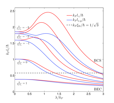
Figure 4: The Cooper pair size defined in Eqn.14 29 along $x$ direction (red lines) ($l_{x}=l_{y}$) and $z$ direction (blue lines) as a function of 3d Rashba SOC strength $\lambda$. Note its non-monotonic behaviors in the BCS side. The effects of SOC are small starting from the BEC side at $\lambda=0$.

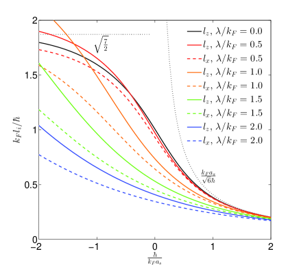
Figure 5: The Cooper pair size $l_{z}>l_{x}=l_{y}$ at a fixed 3d Rashba SOC versus the scattering length. Different colors stand for different SOC strengths. Solid (dashed) lines stand for $l_{z}$ ($l_{x}=l_{y}$). The dark dotted line on the left (right) is its BCS (BEC) limit $\sqrt{7/2}$ ($\frac{k_{F}a_{s}}{\sqrt{6}}$) at $\lambda=0$. On the BCS side, the SOC effects are dramatic, but on the BEC side, the SOC effects are small, all curves converge to the right dotted line $\frac{k_{F}a_{s}}{\sqrt{6}}$ from below.

As shown in Sec.II, the Cooper pair size in Eqn.14 is another characteristic length in Fermi gas system. Formally, one can define the “Cooper pair wavefunction” crossover in the second quantized form by removing the exponential in Eqn.21:

$$\left|g_{cp}\right\rangle = \underset{\boldsymbol{p}}{\sum}^{\prime}\left[w_{\boldsymbol{p}+}e^{-i\varphi_{\boldsymbol{p}}}h_{\boldsymbol{p}+}^{\dagger}h_{\boldsymbol{-p}+}^{\dagger}+w_{\boldsymbol{p}-}e^{i\varphi_{\boldsymbol{p}}}h_{\boldsymbol{p}-}^{\dagger}h_{\boldsymbol{-p}-}^{\dagger}\right]\left|0\right\rangle$$ (26)

$$= \underset{\boldsymbol{p}}{\sum}^{\prime}[g_{\uparrow\downarrow}\left(\boldsymbol{p}\right)c_{\boldsymbol{p}\uparrow}^{\dagger}c_{\boldsymbol{-p}\downarrow}^{\dagger}+g_{\downarrow\uparrow}\left(\boldsymbol{p}\right)c_{\boldsymbol{p}\downarrow}^{\dagger}c_{\boldsymbol{-p}\uparrow}^{\dagger}$$

$$+g_{\uparrow\uparrow}\left(\boldsymbol{p}\right)c_{\boldsymbol{p}\uparrow}^{\dagger}c_{\boldsymbol{-p}\uparrow}^{\dagger}+g_{\downarrow\downarrow}\left(\boldsymbol{p}\right)c_{\boldsymbol{p}\downarrow}^{\dagger}c_{\boldsymbol{-p}\downarrow}^{\dagger}]\left|0\right\rangle,$$

which only has two paired electrons with both singlet and triplet pairing. In Eqn.26, we have used Eqn.17 and found:

$$g_{\uparrow\downarrow}\left(\boldsymbol{p}\right) = -\frac{1}{2}\left(w_{\boldsymbol{p}+}+w_{\boldsymbol{p}-}\right)=-g_{\downarrow\uparrow}\left(-\boldsymbol{p}\right)=-g_{\downarrow\uparrow}\left(\boldsymbol{p}\right),$$

$$g_{\uparrow\uparrow}\left(\boldsymbol{p}\right) = \frac{1}{2}\left(w_{\boldsymbol{p}+}-w_{\boldsymbol{p}-}\right)e^{-i\varphi_{\boldsymbol{p}}}=-g_{\downarrow\downarrow}^{\ast}\left(\boldsymbol{p}\right).$$ (27)

The corresponding first quantized form of Eqn.26 in real space is:

$$g_{cp}(\vec{r}) = g_{\uparrow\downarrow}(\vec{r})(|\uparrow\downarrow\rangle-|\downarrow\uparrow\rangle)$$ (28)

$$+ g_{\uparrow\uparrow}(\vec{r})|\uparrow\uparrow\rangle-g^{*}_{\uparrow\uparrow}(\vec{r})|\downarrow\downarrow\rangle,$$

where $g_{\alpha\beta}(\vec{r})=\sum_{\vec{p}}e^{i\vec{p}\cdot\vec{r}}g_{\alpha\beta}(\vec{p}),\alpha,\beta=\uparrow,\downarrow$. Compared to Eqn.11, one can see that there are two extra equal-spin $p_{x}\pm ip_{y}$ pairing componentslegg similar to the $A$-phase of ${}^{3}He$.

It is easy to see that the Cooper pair size along the $i$ direction in Eqn.14 can be expressed as:

$$l_{i}^{2}=\frac{\left\langle g_{cp}\right|r_{i}^{2}\left|g_{cp}\right\rangle}{\left\langle g_{cp}|g_{cp}\right\rangle},~{}~{}~{}~{}i=x,y,z,$$ (29)

which has a clear physical meaning: the Cooper pair size is the “average size” of the Cooper pair wavefunction Eqn.28. Shown in Fig.4 is the the Cooper pair size along different directions versus the SOC strength. In sharp contrast to the pairing length, it is non-monotonic uncover in the BCS side $a_{s}<0$, so may not be a good quantity to characterize the BCS to BEC crossover. Furthermore, it may not be an experimentally detectable quantity anyway.

In the absence of the SOC when $\lambda=0$, there is only a singlet pairing, Eqn.29 is simplified to:

$$l_{i}^{2}(\lambda=0)=\frac{\hbar^{2}\underset{\boldsymbol{k}}{\sum}\left(1-\frac{\xi_{\boldsymbol{k}}}{E_{\boldsymbol{k}}}\right)^{2}\frac{k^{2}}{m^{2}}}{3\underset{\boldsymbol{k}}{\sum}\left(E_{\boldsymbol{k}}-\xi_{\boldsymbol{k}}\right)^{2}}.$$ (30)

In the weak coupling (BCS) limit (i.e.$\frac{\hbar}{k_{F}a_{s}}\longrightarrow-\infty$), $\mu=E_{F}$ and $\Delta\rightarrow 0$, one finds $l_{x,y,z}\longrightarrow\sqrt{\frac{7}{2}}\frac{\hbar}{k_{F}}$ which is nothing but the inter-particle distance, in sharp contrast to the pairing length which is nothing but the coherence length. Using $l_{0BCS}\sim\frac{\hbar^{2}k_{F}}{2m\epsilon_{F}},\xi_{0BCS}\sim\frac{\hbar^{2}k_{F}}{2m\Delta_{0}}$, one can see their ratio $l_{0BCS}/\xi_{0BCS}\sim\Delta_{0}/\epsilon_{F}=\frac{8}{e^{2}}e^{\frac{\pi\hbar}{2k_{F}a_{s}}}\longrightarrow 0$. For conventional superconductors $l_{0BCS}/\xi_{0BCS}\sim 10^{-4}$ which indicates that there are about $10^{4}$ other Cooper pairs inside a given Cooper pair. However, for high $T_{c}$ superconductors legg ; hightc , $l_{0BCS}/\xi_{0BCS}\sim 10^{-1}$ which indicates that they are quite close to the BCS to BEC crossover, but still in the BCS side.

In the BEC limit, we find $l_{i}\rightarrow\frac{a_{s}}{\sqrt{6}}$ which also recovers the two-body scattering length Eqn.32factor . So $l_{0BCS}/\xi_{0BCS}=1$ in the strong BEC limit. This should be expected because the Cooper pair wavefunction is nothing but the two electrons component of the many-body wavefunction, so both lengths have to be the same in the strong BEC limit.

The Cooper pair sizes along different directions versus the scattering length is shown in Fig.5 which is complementary to Fig.4

III.4 Contrast with two-body wavefunctions

The 2-body wavefunction with a 3d Rashba SOC was worked out in twobody by solving a 2-body Schrodinger equation superbook . It is instructive to compare the many-body wave functions Eqn.21 and the Cooper pair wavefunction Eqn.27 with the corresponding two-body wave functions (see the extreme oblate case in twobody ). They all have the same symmetries, namely:

$$\psi_{\uparrow\downarrow}\left(\boldsymbol{p}\right) = -\psi_{\downarrow\uparrow}\left(\boldsymbol{p}\right),~{}~{}~{}~{}g_{\uparrow\downarrow}\left(\boldsymbol{p}\right)=-g_{\downarrow\uparrow}\left(\boldsymbol{p}\right),$$

$$\psi_{\uparrow\uparrow}\left(\boldsymbol{p}\right) = -\psi_{\downarrow\downarrow}^{\ast}\left(\boldsymbol{p}\right),~{}~{}~{}~{}g_{\uparrow\uparrow}\left(\boldsymbol{p}\right)=-g_{\downarrow\downarrow}^{\ast}\left(\boldsymbol{p}\right).$$ (31)

However, they have quite different behaviors. It was shown that in the absence of the SOC when $\lambda=0$, there exist a bound state in the BEC side only with $a_{s}>0$, the bound state has only a singlet component $\psi_{0}(\vec{r})=\frac{1}{r}e^{-r/a_{s}}$ with a binding energy $E_{b}=\frac{\hbar^{2}}{ma_{s}}$. It is easy to see the size of the bound state:

$$b(\lambda=0)=\frac{\left\langle\psi_{0}\right|r^{2}\left|\psi_{0}\right\rangle}{\left\langle\psi_{0}|\psi_{0}\right\rangle}=\frac{a_{s}}{\sqrt{2}},$$ (32)

which is identical to both the pairing size Eqn.9 and the Cooper-pair size Eqn.14 in the BEC limit factor . As shown in Fig.1, in the absence of the SOC when $\lambda=0$, the pairing length $\xi_{i}$ and Cooper pair size $l_{i}$ are well defined in both the BCS and BEC limit.

However, as shown in twobody , a non-zero SOC strength $\lambda\neq 0$ will always lead to a two-body bound state at any $a_{s}$, extending the $b(\lambda=0)$ in Eqn.32 to a non-zero $\lambda$ can be easily calculated using the two body wavefunctions in twobody ; colliso . Any non-zero SOC strength, as shown in Fig.1, leads to $\xi_{z}>\xi_{x}=\xi_{y}$ and $l_{z}>l_{x}=l_{y}$. In the BCS side, $\xi_{i}$ and $l_{i}$ display dramatically different behaviors. While in the BEC limit both $\xi_{i}$ and $l_{i}$ converge to the size of the two-body bound state. This is expected, in the strong BEC limit, the overlap between the two-body wavefunction and the many-body wavefunction must be the same as that between the two-body wavefunction and the Cooper-pair wavefunction.

IV 3D Fermi gas with an isotropic Weyl SOC

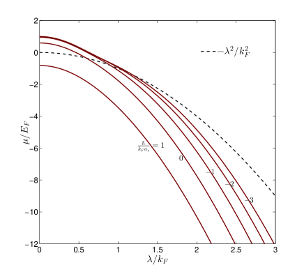
Figure 6: The chemical potential $\mu$ versus the 3D isotropic Weyl SOC strength $\lambda$ for different scattering lengths. The black dashed line $\mu_{0}=-\frac{\lambda^{2}}{2m}$is the chemical potential at the bottom of single particle spectrum. Starting from the BCS side at $\lambda=0$, as $\lambda$ increases, the $\mu$ drops below $\mu_{0}$ indicating a crossover from BCS to BEC.

The 3d Weyl SOC term can be written as

$$V_{Weyl} = \frac{\lambda}{m}\underset{\boldsymbol{p}}{\sum}[p_{\perp}\left(e^{-i\varphi_{\boldsymbol{p}}}c_{\boldsymbol{p}\uparrow}^{\dagger}c_{\boldsymbol{p}\downarrow}+e^{i\varphi_{\boldsymbol{p}}}c_{\boldsymbol{p}\downarrow}^{\dagger}c_{\boldsymbol{p}\uparrow}\right)$$ (33)

$$+ p_{z}\left(c_{\boldsymbol{p}\uparrow}^{\dagger}c_{\boldsymbol{p}\uparrow}-c_{\boldsymbol{p}\downarrow}^{\dagger}c_{\boldsymbol{p}\downarrow}\right)].$$

The single particle part in Hamiltonian Eqn.1 can be diagonalized in the helicity bases as $H_{0}=\underset{\boldsymbol{p}}{\sum}\left(\xi_{\boldsymbol{p}+}h_{\boldsymbol{p}+}^{\dagger}h_{\boldsymbol{p}+}+\xi_{\boldsymbol{p}-}h_{\boldsymbol{p}-}^{\dagger}h_{\boldsymbol{p}-}\right)$ where $\xi_{\boldsymbol{p}\pm}=\frac{p^{2}}{2m}\pm\frac{\lambda p}{m}-\mu$ and the helicity operators:

$$h_{\boldsymbol{p}+} = \sqrt{\frac{1}{2}}\left[\sqrt{\frac{p+p_{z}}{p}}c_{\boldsymbol{p}\uparrow}+\sqrt{\frac{p-p_{z}}{p}}e^{-i\varphi_{\boldsymbol{p}}}c_{\boldsymbol{p}\downarrow}\right],$$

$$h_{\boldsymbol{p}-} = \sqrt{\frac{1}{2}}\left[\sqrt{\frac{p-p_{z}}{p}}e^{i\varphi_{\boldsymbol{p}}}c_{\boldsymbol{p}\uparrow}-\sqrt{\frac{p+p_{z}}{p}}c_{\boldsymbol{p}\downarrow}\right].$$ (34)

In the mean-field theory, the total Hamiltonian can also be diagonalized as Eqn.18, and the quasiparticle excitation energy $E_{\boldsymbol{p}\pm}=\sqrt{\xi_{\boldsymbol{p}\pm}^{2}+\left|\Delta_{0}\right|^{2}}$, and the Bogoliubov quasi-particle operators take the same form as Eqn.19. At zero temperature, the two self-consistent equations also take the same form as Eqn.20 with the corresponding $\xi_{\boldsymbol{p}\pm}$ and $E_{\boldsymbol{p}\pm}$ defined above. Solving them leads to the chemical potential shown in Fig.6. Similar to Fig.1, the Weyl SOC also drives a new crossover from BCS to BEC.

IV.1 Pairing length

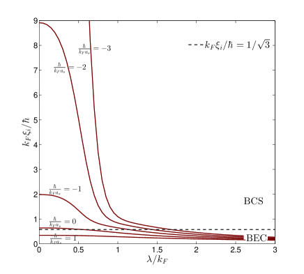
Figure 7: From the BCS side at $\lambda=0$, the pairing length $\xi_{x}=\xi_{y}=\xi_{z}$ of 3d Weyl SOC decreases quickly and monotonically as the $\lambda$ increases and drop below the dashed line. It describe precisely the new BCS to BEC crossover driven by the SOC strength. The dashed line is a contrasting line where $k_{F}\xi_{0}=\hbar$ (for each component, $k_{F}\xi_{0i}=\hbar/\sqrt{3}$). From the BEC side at $\lambda=0$, the effects of SOC are small.

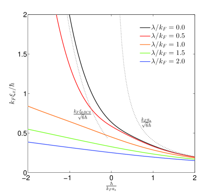
Figure 8: The pairing lengths $\xi_{i}$ of 3d Weyl SOC at a fixed SOC versus the scattering length. Different colors stand for different SOC strengths. The dark dotted line on the left (right) is its BCS (BEC) limit $\frac{1}{\sqrt{6}}k_{F}\xi_{0BCS}=\frac{1}{8\sqrt{6}e^{2}}e^{-\frac{\pi\hbar}{2k_{F}a_{s}}}$ ($\frac{k_{F}a_{s}}{\sqrt{6}}$) at $\lambda=0$. On the BCS side, the SOC effects are dramatic, but on the BEC side, the SOC effects are small, all curves converge to the right dotted line $\frac{k_{F}a_{s}}{\sqrt{6}}$ from below. Compare with Fig.3.

The wavefunction stays the same as Eqn.21 with the corresponding $\xi_{\boldsymbol{p}\pm}$ and $E_{\boldsymbol{p}\pm}$ defined above. Similar to Sec.III-B, we can determine the singlet pairing amplitude:

$$\psi_{\begin{subarray}{c}\uparrow\downarrow\\ \downarrow\uparrow\end{subarray}}\left(\boldsymbol{p}\right) = \frac{\left\langle BCS\right|c_{\boldsymbol{p}\uparrow}^{\dagger}c_{-\boldsymbol{p}\downarrow}^{\dagger}\left|BCS\right\rangle}{\left\langle BCS|BCS\right\rangle}$$

$$= \mp\frac{1}{2}\left(\frac{w_{\boldsymbol{p}+}}{1+w_{\boldsymbol{p}+}^{2}}+\frac{w_{\boldsymbol{p}-}}{1+w_{\boldsymbol{p}-}^{2}}\right)$$

$$- \frac{1}{2}\left(\frac{w_{\boldsymbol{p}+}}{1+w_{\boldsymbol{p}+}^{2}}-\frac{w_{\boldsymbol{p}-}}{1+w_{\boldsymbol{p}-}^{2}}\right)\frac{p_{z}}{p},$$

and triplet pairing amplitude:

$$\psi_{\uparrow\uparrow}\left(\boldsymbol{p}\right) = \frac{\left\langle BCS\right|c_{\boldsymbol{p}\uparrow}^{\dagger}c_{-\boldsymbol{p}\uparrow}^{\dagger}\left|BCS\right\rangle}{\left\langle BCS|BCS\right\rangle}$$

$$= \frac{1}{2}\left(\frac{w_{\boldsymbol{p}+}}{1+w_{\boldsymbol{p}+}^{2}}-\frac{w_{\boldsymbol{p}-}}{1+w_{\boldsymbol{p}-}^{2}}\right)\frac{p_{\perp}}{p}e^{i\varphi_{\boldsymbol{p}}}=-\psi_{\downarrow\downarrow}^{\ast}\left(\boldsymbol{p}\right),$$

where $w_{\boldsymbol{p}\pm}=\sqrt{\frac{E_{\boldsymbol{p}\pm}-\xi_{\boldsymbol{p}\pm}}{E_{\boldsymbol{p}\pm}+\xi_{\boldsymbol{p}\pm}}}$.

The pairing length $\xi_{i}$ can be calculated using Eqn.9 and is shown in Fig.7. As the Weyl SOC strength increases, in the BCS side, the pairing length along any direction decreases monotonically and quickly, then drop below the dashed line. In the BEC side, the effects of the SOC strength are quite small. This is the most direct evidence that the Weyl SOC can also drive a crossover from BCS to BEC and can be directly detected by the MIT type of experiment mitdiss .

The pairing lengths versus the scattering length is shown in Fig.8 which is complementary to Fig.7

IV.2 Cooper pair size

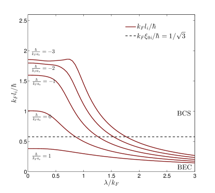
Figure 9: The Cooper pair size $l_{x}=l_{y}=l_{z}$ of 3d Weyl SOC as a function of $\lambda$. Note its non-monotonic behavior at the BCS side. The SOC effects on the BEC side are small.

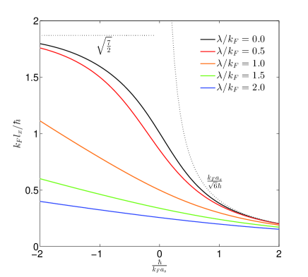
Figure 10: The Cooper pair size $l_{i}$ of 3d Weyl SOC at a fixed SOC versus the scattering length. Different colors stand for different SOC strengths. The dark dotted line on the left (right) is its BCS (BEC) limit $\sqrt{7/2}$ ($\frac{k_{F}a_{s}}{\sqrt{6}}$) at $\lambda=0$. On the BCS side, the SOC effects are dramatic, but on the BEC side, the SOC effects are small, all curves converge to the right dotted line $\frac{k_{F}a_{s}}{\sqrt{6}}$ from below. Compare with Fig.5.

The Cooper pair wave function takes the same form as Eqn.26 in the second quantized form and Eqn.28 in the first quantized form with the corresponding $\xi_{\boldsymbol{p}\pm}$ and $E_{\boldsymbol{p}\pm}$ defined above. All the components can be written as:

$$g_{\uparrow\downarrow}\left(\boldsymbol{p}\right) = -\frac{1}{2}\left(w_{\boldsymbol{p}+}+w_{\boldsymbol{p}-}\right)-\frac{1}{2}\left(w_{\boldsymbol{p}+}-w_{\boldsymbol{p}-}\right)\frac{p_{z}}{p}=-g_{\downarrow\uparrow}\left(-\boldsymbol{p}\right),$$

$$g_{\downarrow\uparrow}\left(\boldsymbol{p}\right) = \frac{1}{2}\left(w_{\boldsymbol{p}+}+w_{\boldsymbol{p}-}\right)-\frac{1}{2}\left(w_{\boldsymbol{p}+}-w_{\boldsymbol{p}-}\right)\frac{p_{z}}{p},$$

$$g_{\uparrow\uparrow}\left(\boldsymbol{p}\right) = \frac{1}{2}\left(w_{\boldsymbol{p}+}-w_{\boldsymbol{p}-}\right)\frac{p_{\perp}}{p}e^{-i\varphi_{\boldsymbol{p}}}=-g_{\downarrow\downarrow}^{\ast}\left(\boldsymbol{p}\right).$$ (35)

The Cooper-pair size can be evaluated using Eqn.29 and plotted in Fig.9. Its non-monotonic behaviors at the BCS side indicate it may not be a good quantity to characterize the crossover.

The Cooper pair sizes versus the scattering length is shown in Fig.10 which is complementary to Fig.9.

IV.3 Contrast with the two-body wavefunctions

To explore the relations between the many-body wavefunctions or the “Cooper-pair” wavefunction studied in this section and the two body wavefunctions in twobody , it is convenient to introduce the spin eigenstate along the momentum $\frac{\boldsymbol{p}}{p}=(\sin\theta\cos\varphi,\sin\theta\sin\varphi,\cos\theta)$:

$$\left|\uparrow\right\rangle_{\boldsymbol{p}} = e^{-i\frac{\varphi}{2}}\cos\frac{\theta}{2}\left|\uparrow\right\rangle+e^{i\frac{\varphi}{2}}\sin\frac{\theta}{2}\left|\downarrow\right\rangle,$$

$$\left|\downarrow\right\rangle_{\boldsymbol{p}} = e^{-i\frac{\varphi}{2}}\sin\frac{\theta}{2}\left|\uparrow\right\rangle-e^{i\frac{\varphi}{2}}\cos\frac{\theta}{2}\left|\downarrow\right\rangle,$$

then to express the many-body wavefunctions in terms of the spin eigenstates along the momentum $\vec{p}$:

$$g_{\uparrow\downarrow}\left(\boldsymbol{p}\right)\left|\uparrow\downarrow\right\rangle+g_{\downarrow\uparrow}\left(\boldsymbol{p}\right)\left|\downarrow\uparrow\right\rangle+g_{\uparrow\uparrow}\left(\boldsymbol{p}\right)\left|\uparrow\uparrow\right\rangle+g_{\downarrow\downarrow}\left(\boldsymbol{p}\right)\left|\downarrow\downarrow\right\rangle$$ (36)

$$= -\frac{1}{2}\left(w_{p+}+w_{p-}\right)\left(\left|\uparrow\downarrow\right\rangle-\left|\downarrow\uparrow\right\rangle\right)+\frac{1}{2}\left(w_{p+}-w_{p-}\right)\times$$

$$\left[\frac{p_{x}-ip_{y}}{p}\left|\uparrow\uparrow\right\rangle-\frac{p_{z}}{p}(\left|\uparrow\downarrow\right\rangle+\left|\downarrow\uparrow\right\rangle)-\frac{p_{x}+ip_{y}}{p}\left|\downarrow\downarrow\right\rangle\right]$$

$$= -\frac{1}{2}\left(w_{p+}+w_{p-}\right)\left(\left|\uparrow\downarrow\right\rangle-\left|\downarrow\uparrow\right\rangle\right)$$

$$+ \frac{1}{2}\left(w_{p+}-w_{p-}\right)\left(\left|\uparrow\downarrow\right\rangle_{\boldsymbol{p}}+\left|\downarrow\uparrow\right\rangle_{\boldsymbol{p}}\right)$$

$$\equiv g_{a}\left(p\right)\left(\left|\uparrow\downarrow\right\rangle-\left|\downarrow\uparrow\right\rangle\right)+g_{s}\left(p\right)\left(\left|\uparrow\downarrow\right\rangle_{\boldsymbol{p}}+\left|\downarrow\uparrow\right\rangle_{\boldsymbol{p}}\right),$$

where the components $g_{a}\left(p\right)$ and $g_{s}\left(p\right)$ are independent on direction of $\boldsymbol{p}$ (i.e. $\theta$ and $\varphi$). Compared to Eqn.11, one can see that there are three extra $p_{x}\pm ip_{y}$ and $p_{z}$ pairing componentslegg similar to the $B$-phase of superfluid ${}^{3}He$. This fact should be contrasted to Eqn.28 where there are only two extra equal-spin $p_{x}\pm ip_{y}$ pairing componentslegg similar to the $A$-phase of superfluid ${}^{3}He$.

Fourier transforming the “Cooper-pair” wavefunction Eqn.36 to real space and comparing with the two body wavefunction in the spherical case in twobody , we find that they have the same symmetry. In fact, a similar relation between the wavefunctions (or order parameters) in real space and those in the helicity momentum basis were derived for magnetic transitions in repulsively interacting Fermi gas replusive2 .

V 2D Fermi gas with a Rashba SOC

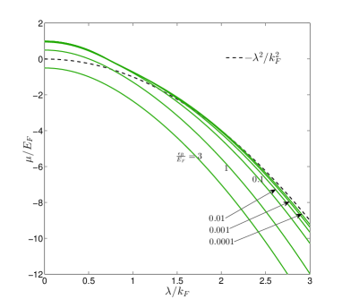
Figure 11: The chemical potential $\mu$ versus $\lambda$ in 2D isotropic SOC system for different scattering lengths. The dashed line is the minimum energy of the single particle $\mu_{0}=-\frac{\lambda^{2}}{2m}$. On the BCS side, as $\lambda$ increases, the $\mu$ drops below $\mu_{0}$ indicating a crossover from a BCS to BEC crossover.

A 2D Rashba SOC term can be written as

$$V_{2d-ra}=\frac{\lambda}{m}\underset{\boldsymbol{p}}{\sum}p\left[e^{-i\varphi_{\boldsymbol{p}}}c_{\boldsymbol{p}\uparrow}^{\dagger}c_{\boldsymbol{p}\downarrow}+e^{i\varphi_{\boldsymbol{p}}}c_{\boldsymbol{p}\downarrow}^{\dagger}c_{\boldsymbol{p}\uparrow}\right],$$ (37)

where $\lambda$ is the strength of SOC, $p=\sqrt{p_{x}^{2}+p_{y}^{2}}$ and $\varphi_{\boldsymbol{p}}=Arg\left(p_{x}+ip_{y}\right)$. Note that the space is 2d, but the spin is still $SU(2)$ with the 3 generators.

The BCS theory in two dimension has been studied by several worksxi ; xi2 with different focus. The calculations are similar to the 3d Rashba case in Sec.III with the momentum $\vec{p}$ confined to be the 2d momentum $\vec{p}_{\perp}$, or similar to the 3d Weyl case in Sec.IV by setting $p_{z}=0$. Eqn.16,17, 18, 19 follow. The two self-consistent equations Eqn.20 also hold with the crucial difference that the interaction need to be regularized by a bound state energy $\epsilon_{B}$ at 2d, instead of a scattering length $a_{s}$ in 3d: $\frac{1}{g}=-\frac{1}{V}\underset{\boldsymbol{p}}{\sum}\frac{1}{2\epsilon_{\boldsymbol{p}}+\epsilon_{B}}$. Solving them leads to the chemical potential $\mu$ shown in Fig.11.

V.1 Pairing length

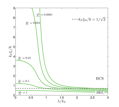
Figure 12: The 2d pairing length defined in Eqn.9 ($\xi_{x}=\xi_{y}$) as a function of $\lambda$. At the BCS side, it decreases quickly and monotonically as the $\lambda$ increases and drop below the dashed line. It describe precisely the new BCS to BEC crossover driven by the SOC strength. The dashed line is a guidance line where $k_{F}\xi_{0}=\hbar$ (averagely, $k_{F}\xi_{0i}=\hbar/\sqrt{2}$). At the BEC side, the effects of SOC are small.

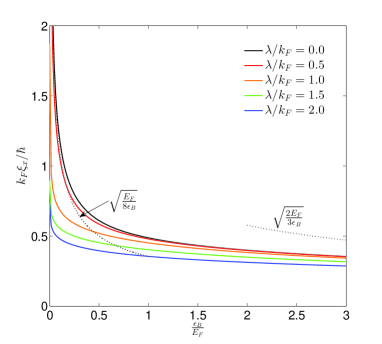
Figure 13: The 2d pairing lengths $\xi_{x}=\xi_{y}$ at a fixed SOC versus the scattering length. Different colors stand for different SOC strengths. The black dotted line on the left (right) is its BCS (BEC) limit $\sqrt{\frac{E_{F}}{8\epsilon_{B}}}$ ($\sqrt{\frac{2E_{F}}{3\epsilon_{B}}}$) at $\lambda=0$. On the BCS side, the SOC effects are dramatic, but on the BEC side, the SOC effects are small, all curves converge to the right dotted line $\sqrt{\frac{2E_{F}}{3\epsilon_{B}}}$ from below.

When calculating the pairing length, Eqns.21, 23, 24 still hold. For $\lambda\neq 0$, only numerical results are available and are shown in Fig.12. We can see that in the BCS limit at $\lambda=0$, as the strength of SOC increases for a fixed interaction strength $\frac{\epsilon_{B}}{E_{F}}$, the pair size decreases monotonically and sharply, then below the the reference line. Here, we also plot a reference line by taking $k_{F}\xi_{0}=\hbar$ (for each component, $k_{F}\xi_{0i}=\frac{\hbar}{\sqrt{2}}$) to qualitatively observe the BCS to BEC crossover behavior. In the BEC limit, the effects of SOC are small.

Setting $\lambda=0$, one can easily solve the self-consistent equations and find $\mu=E_{F}-\frac{\left|\epsilon_{B}\right|}{2}$ and $\Delta=\sqrt{2\left|\epsilon_{B}\right|E_{F}}$. When $\lambda=0$, Eqn.25 at $d=3$ should be replaced by xi ; xi2 :

$$\xi_{x,y}^{2}(\lambda=0) = \frac{\hbar^{2}4\int dpp^{d+1}\frac{\xi_{\boldsymbol{p}}^{2}}{E_{\boldsymbol{p}}^{6}}}{\left(2m\right)^{2}d\int dp\frac{p^{d-1}}{E_{\boldsymbol{p}}^{2}}}$$ (38)

$$= \frac{\hbar^{2}}{4\left(2m\Delta\right)}\left(\eta+\frac{\eta^{2}+2}{\eta^{2}+1}\frac{1}{\frac{\pi}{2}+\arctan\eta}\right),$$

where $\eta=\frac{\mu}{\Delta}$. Because of different dimensions, this analytical expression is very different from Eqn.25 in 3d. In the BCS limit (i.e. $\frac{\epsilon_{B}}{E_{F}}\longrightarrow 0$), $\eta=\frac{1}{\sqrt{2}}\sqrt{\frac{E_{F}}{\left|\epsilon_{B}\right|}}\longrightarrow\infty$, $k_{F}\xi_{x,y}\longrightarrow\sqrt{\frac{E_{F}}{8\left|\epsilon_{B}\right|}}$ which diverges. In the BEC limit (i.e. $\frac{\left|\epsilon_{B}\right|}{E_{F}}\longrightarrow\infty$), $\mu=-\frac{\left|\epsilon_{B}\right|}{2}$ and $\eta=-\frac{1}{2\sqrt{2}}\sqrt{\frac{\left|\epsilon_{B}\right|}{E_{F}}}\longrightarrow-\infty$, $k_{F}\xi_{x,y}\rightarrow\sqrt{\frac{3}{2}\frac{E_{F}}{\left|\epsilon_{B}\right|}}$.

Shown in Fig.13 is the pairing length versus the scattering length which is complementary to Fig.12.

V.2 Cooper pair size

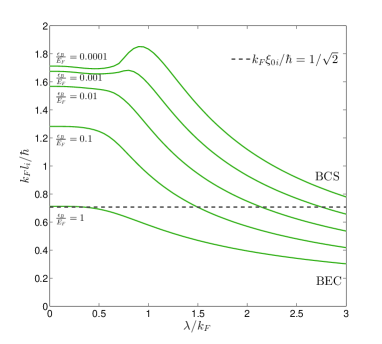
Figure 14: The 2d Cooper pair size $l_{x}=l_{y}$ as a function of $\lambda$. Note its non-monotonic behavior at the BCS side.

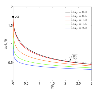
Figure 15: The 2d Cooper pair size $l_{x}=l_{y}$ at a fixed SOC versus the scattering length. Different colors stand for different SOC strengths. The black dotted line on the left (right) is its BCS (BEC) limit $\sqrt{3}$ ($\sqrt{\frac{2E_{F}}{3\epsilon_{B}}}$) at $\lambda=0$. On the BCS side, the SOC effects are dramatic, but on the BEC side, the SOC effects are small, all curves converge to the right dotted line $\sqrt{\frac{2E_{F}}{3\epsilon_{B}}}$ from below.

When calculating the Cooper-pair size, Eqns. 26, 27, 28, 29 still hold. Shown in Fig.14 is how the Cooper-pair size changes with $\lambda$. Once more, its non-monotonic behaviors at the BCS side indicate it may not be a good quantity to characterize the BCS to BEC crossover.

When $\lambda=0$, Eqn.30 at $d=3$ should be replaced by:

$$l_{i}^{2}(\lambda=0)=\frac{3\hbar^{2}\left[\ln 2-\frac{1}{2}-\eta\left(\frac{\pi}{2}+\arctan\eta\right)-\ln\left(1-\frac{\eta}{\sqrt{\eta^{2}+1}}\right)+\eta\left(\eta+\sqrt{\eta^{2}+1}\right)\right]}{2m\Delta\left[\eta^{3}+\left(\eta^{2}+1\right)^{\frac{3}{2}}+\frac{3}{2}\eta\right]},$$ (39)

where $\eta=\frac{\mu}{\Delta}$. In the BCS limit (i.e.$\frac{\epsilon_{B}}{E_{F}}\longrightarrow 0$), one get $l_{x,y}\longrightarrow\sqrt{3}\frac{\hbar}{k_{F}}$ which is nothing but the inter-particle distance, so it goes to a finite value, in sharp contrast to the pairing length which diverges. In fact, $l/\xi\sim\Delta_{0}/\epsilon_{F}\rightarrow 0$ in the BCS limit. In the BEC limit (i.e.$\frac{\left|\epsilon_{B}\right|}{E_{F}}\longrightarrow\infty$), one find $k_{F}l_{x,y}=\sqrt{\frac{2E_{F}}{3\left|\epsilon_{B}\right|}}$ which is identical to $k_{F}\xi_{x,y}$ in the BEC limit as it should be.

Shown in Fig.15 is the Cooper pair size at various fixed SOC strengths versus the bound state energies $\epsilon_{B}/E_{F}$ which is complementary to Fig.14.

VI Applications to 2d superconductor and semi-conductor systems

In various 3d condensed matter systems ahe ; kitpconf , the 3d SOC usually take $\lambda(\vec{k}\times\vec{\sigma})\cdot\nabla V$ which is quite different form than Weyl or Rashba form studied in Sec.III and IV by keeping the inversion symmetry. It may be interesting to see if such a 3d inversion symmetric SOC can also drive a BCS to BEC crossover.

Eqn.1 with the 2D Rashba SOC term Eqn.37 may also describe 2d bright exciton with total angular momentum $J=\pm 1$ in electron-hole semiconductor bilayer systems and electron pairings in 2d non-centrosymmetric superconductorssocsemi ; niu ; wu . It was known that in a 2d semiconductor electron gas, the 2d Rashiba SOC strength depends on the electric field, presence of adatoms at the boundary, atomic weight and atomic shells involved socsemi ; Kane ; Zhang . In the surface of non-centrosymmetric superconductors, the strong near surface electric fields lead to a 2d Rashba SOC quite similar to the 2d superconducting fullerene and polyacene crystals in the field-effect-transistor geometry socsemi . So the 2d Rashba SOC strength in the two condensed matter systems can also be tuned by adjusting various surface geometries. So the results achieved on the BCS to BEC crossover tuned by the 2d Rashba strength in the section V should also apply to these condensed matter systems. In Ref.power ; squ ; excitoncorr ; exciton2 , the authors ignored the spins of the electrons and holes, therefore also the possible Rashba SOC. As shown at the end of excitoncorr , the bright excitons couple to the one photon process with the polarization $\sigma=\pm$. By incorporating the coupling between the 2d bright excitons subject to the 2d Rashba SOC studied in Sec.V and the 3d emitted photons with the two polarizations, it is interesting study how the emitted photon characteristics change across the new BCS to BEC crossover driven by the 2d Rashiba SOC.

VII Discussions and Conclusions

The new BCS to BEC crossover driven by the SOC strength has been studied by previous authors from the overlap between “Cooper-pair wavefunction” and two body wavefunction crossover , also from the “Cooper-pair size” right at the Feshbach resonance zhai . In this paper, we investigate the new BCS to BEC crossover from fundamental and physical points of view. At the mean field level, we studied the dependence of chemical potential, pairing length, Cooper-pair size on the SOC strength for three kinds of Fermi gases with 3d Rashba, 3d Weyl and 2d Rashba SOC respectively. We explicitly demonstrated the new BCS to BEC crossover driven by the SOC strength in all the three cases by monitoring the monotonic decreasing of chemical potential and the pairing length. We show that the most relevant wavefunction is the many body wave function instead of the “Cooper-pair wavefunction” or two body wavefunction, the most relevant length is the pairing length instead of the“Cooper-pair size” or the two-body bound state size. Among the three lengths, only the pairing length is the experimentally detectable length.

We can summarize the main differences among the pairing length, the Cooper-pair size and the two-body size in the following: In the absence of SOC, in the BCS limit, the pairing length goes to the coherence length $\xi(\lambda=0)=\hbar v_{F}/\Delta_{0}$, while the Cooper-pair size goes to the inter-particle distance $l(\lambda=0)\sim 1/k_{F}$. Their ratio $l(\lambda=0)/\xi(\lambda=0)\sim\Delta_{0}/\epsilon_{F}$. For conventional superconductors superbook , $l(\lambda=0)/\xi(\lambda=0)\sim 10^{-4}$, so they are well inside the BCS limit. The BCS mean field theory work well, quantum and classical fluctuation effects can be neglected except very close to the critical transitions at finite temperatures. For high temperature superconductors legg ; hightc , $l(\lambda=0)/\xi(\lambda=0)\sim 10^{-1}$, so they are quite close to BCS to BEC crossover, but still in the BCS limit with well defined Fermi surface. So quantum and classical fluctuation effects can not be ignored legg . In the BEC limit, they both get to the two-body bound state size, therefore $l(\lambda=0)/\xi(\lambda=0)\sim 1$. The results on $\xi$ in Eqn.25 at 3d melo and Eqn.38 at 2d xi ; xi2 are not new, but the results on $l$ in Eqn.30 at 3d and Eqn.39 are new and show completely different behaviors than $\xi$. It is very instructive to compare the two different length scales. In the presence of SOC, on the BCS side, the pairing length $\xi_{i}(\lambda),i=x,y,z$ decrease monotonically and quickly move into the BEC regime, so can be used to characterize the BCS to BEC crossover quantitatively. Furthermore it can be detected by RF dissociation spectra experiment. While $l_{i}(\lambda)$ shows non-monotonic behaviors, so can not be used to characterize the BCS to BEC crossover even qualitatively. Furthermore it is not an experimentally measurable quantity.

In a future publication, we will compute the fluctuation corrections to the mean filed theory results on the pairing length achieved in this paper. One can achieve the goal by calculating the fermion pairing correlation function Eqn.8 using $1/N$ expansion dicke1 ; dicke2 . It was known the quantum fluctuation effects are important near the BCS to BEC regime. It may also be interesting to extend the zero temperature results on the pairing length to finite temperatures whose effects are especially important to 2d Rashba systems studied in Sec.V and VI. However, it is not known how to extend the concepts of Cooper-pair size defined in Eqn.14 beyond mean field results and to finite temperatures. Above all, its definition is based on the explicit form of the mean field state. Therefore, the pairing length is a much more robust concept than the Cooper-pair size. It is also a experimentally measurable quantity through radio-frequency dissociation spectra. Of course, the two-body wavefunction is defined only for two fermions, can not be used to study a many body system anyway. The Cooper-pair size has been evaluated at the mean field through the topological transition in read . As demonstrated in this paper, the pairing length show quite different behaviors than the Cooper-pair size, it maybe useful to study the pairing length through various topological transitions driven by the Zeeman field topo2dra ; topo3d ; luo .

Acknowledgements

We thank Fadi Sun for helpful discussions. YY and JY are supported by NSF-DMR-1161497, NSFC-11174210, Beijing Municipal Commission of Education under Grant No. PHR201107121. WL was supported by the NKBRSFC under grants Nos. 2011CB921502, 2012CB821305, NSFC under grants Nos. 61227902, 61378017, 11311120053.

References

(1) Jinwu Ye, Y. B. Kim, A. J. Millis, B. I. Shraiman, P. Majumdar, and Z. Tešanović, Phys. Rev. Lett. 83, 3737 (1999).
(2) Lev P. Gor’kov and Emmanuel I. Rashba, Phys. Rev. Lett. 87, 037004 (2001).
(3) Wang Yao and Qian Niu, Phys. Rev. Lett. 101, 106401 (2008).
(4) Wu Cong-Jun, Ian Mondragon-Shem, Zhou Xiang-Fa, Chin. Phys. Lett, Vol, 28, 097102 (2011).
(5) M. Z. Hasan and C. L. Kane, Rev. Mod. Phys. 82, 3045 (2010).
(6) X. L. Qi and S. C. Zhang, Rev. Mod. Phys. 83, 1057 (2011).
(7) For example, see “Exotic Phases of Frustrated Magnets” conference held at KITP October 8-12, 2012.
http://online.kitp.ucsb.edu/online/fragnets-c12/
(8) Y. J. Lin, K. Jiménez-García, and I. B. Spielman, Nature (London) 471, 83 (2011).
(9) P. Wang, Z. Q. Yu, Z. Fu, J. Miao, L. Huang, S. Chai, H. Zhai, and J. Zhang, Phys. Rev. Lett. 109, 095301 (2012).
(10) L. W. Cheuk, A. T. Sommer, Z. Hadzibabic, T. Yefsah, W. S. Bakr, and M. W. Zwierlein, Phys. Rev. Lett. 109, 095302 (2012).
(11) For a review, see J. Dalibard, F. Gerbier, G. Juzelinas, and P. Öhberg, Rev. Mod. Phys. 83, 1523 (2011).
(12) B. M. Anderson, I. B. Spielman, and G. Juzeliūnas, Phys. Rev. Lett. 111, 125301 (2013).
(13) Z.-F. Xu, L. You, and M. Ueda, Phys. Rev. A 87, 063634 (2013); Z. -F. Xu and L. You, Phys. Rev. A 85, 043605 (2012).
(14) J. P. Vyasanakere and V. B. Shenoy, Phys. Rev. B 83, 094515 (2011)
(15) J. P. Vyasanakere, S. Zhang and V. B. Shenoy, Phys. Rev. B 84, 014512 (2011).
(16) Z. -Q. Yu and H. Zhai, Phys. Rev. Lett. 107, 195305 (2011).
(17) H. Hu, L. Jiang, X. J. Liu and H. Pu, Phys. Rev. Lett. 107, 195304 (2011).
(18) Lianyi He and Xu-Guang Huang, Phys. Rev. Lett. 108, 145302 (2012).
(19) Kezhao Zhou and Zhidong Zhang, Phys. Rev. Lett. 108, 025301 (2012) [5 pages]
(20) Lianyi He and Xu-Guang Huang, Phys. Rev. B 86, 014511 (2012).
(21) Jayantha P. Vyasanakere and Vijay B. Shenoy, Phys. Rev. A 86, 053617 (2012).
(22) Shang-Shun Zhang, Xiao-Lu Yu, Jinwu Ye, Wu-Ming Liu, Phys. Rev. A 87, 063623 (2013).
(23) Shang-Shun Zhang, Jinwu Ye and Wu-Ming Liu, arXiv:1403.7031.
(24) M. Aidelsburger, et.al, Phys. Rev. Lett. 107, 255301 (2011).
J. Struck, et.al, Science 333, 996 (2011);
Phys. Rev. Lett. 108, 225304 (2012); Nat. Phys., doi: 10.1038/nphys2750 (2013).
(25) M. Aidelsburger, et.al, Phys. Rev. Lett. 111, 185301 (2013); H. Miyake, G. A. Siviloglou, C. J. Kennedy, W. C. Burton and W. Ketterle, Phys. Rev. Lett. 111, 185302 (2013); C. J. Kennedy, G. A. Siviloglou, H. Miyake, W. C. Burton and W. Ketterle, Phys. Rev. Lett. 111, 225301 (2013).
(26) Fa-Di Sun, Xiao-Lu Yu, Jinwu Ye, Heng Fan, W. M. Liu, Scientific Reports 3, 2119 (2013).
(27) Fa-Di Sun, Jinwu Ye and W. M. Liu, Preprint.
(28)P. G. De Gennes, Superconductivity of Metals and Alloys, Perseus
Books Publishing, L.L.C. 1999. In Page 96, the Eqn.14 was evaluated with repect to
two-electrons wavefunction outside a Fermi surface which is the original Cooper-pair problem.
Due to the absence of the Fermi surface, this two-body bound state discussed in twobody still differs from
the original Cooper-pair problem.
(29) A.J. Leggett, Quantum Liquids, Oxford University Press, 2006.
(30) Immanuel Bloch, Jean Dalibard, Wilhelm Zwerger, Rev. Mod. Phys. 80, 885 (2008).
(31) Jinwu Ye, Phys. Rev. Lett. 86, 316 (2001); Phys. Rev. Lett. 87, 227003 (2001); Phys. Rev. B. 65, 214505 (2002).
(32) Jinwu Ye, T. Shi and Longhua Jiang, Phys. Rev. Lett. 103, 177401 (2009);
(33) T. Shi, Longhua Jiang and Jinwu Ye, Phys. Rev. B 81, 235402 (2010)
(34) Jinwu Ye, Fadi Sun, Yi-Xiang Yu and Wuming Liu, Ann. Phys. 329 (2013), 51 C72.
(35) Jinwu Ye, J. Low Temp Phys. 158(5), 882-900 (2010).
For a review, see : Yu Chen, Jinwu Ye and Quang Shan Tian, J. Low Temp Phys. 169 (2012), 149-168.
(36) As shown in Sec.II-B, the reason to put a quotation mark on both “Cooper-pair wavefunction” and “Cooper-pair size”
is that they are not really physical, so may not be really understood as the Cooper-pair wavefunction and Cooper-pair size.
For the illustration purposes, they are evaluated here to compare with the physical pairing length and two-body bound state.
Furthermore, several authors read ; zhai also evaluated this un-physical length in different contexts.
For notation simplicties, we dropped the quotation mark in the following.
(37) J. R. Engelbrecht, M. Randeria, and C. A. R. Sá de Melo, Phys. Rev. B 55, 15153 (1997).
(38) Christian H. Schunck, Yong-il Shin, Andr Schirotzek, Wolfgang Ketterle, Nature 454, 739-743 (7 August 2008).
(39) N. Read and Dmitry Green, Phys. Rev. B 61, 10267 C10297 (2000).
For the purpose of making connections with the p-wave pairing nature of the non-abelian Pfaffian FQHE wavefunction,
the “Cooper-pair wavefunction” is the suitable quantity to compare.
(40) Note that which is exactly
the size of the two-body bound state in Eqn.32.
(41) In Ref.zhai , only the at the resonance was calculated.
Our curve in Fig.4 at the resonance recovers their results. But as indicated in the text,
the non-monotonic behaviors of discovered in the Fig.4 can only be seen in the BCS side . Of course, as indicated in the text,
the can not be used to characetrize the BCS to BEC crossover and is not an experimental measurable quantity anyway.
(42) M. Randeria, J.-M. Duan, and L.-Y. Shieh, Phys. Rev. B 41, 327 (1990).
(43) V. M. Loktev, R. M. Quick, and S. G. Sharapov, Phys. Rep. 349,
1 (2001).
(44) Jinwu Ye and C. L. Zhang, Phys. Rev. A 84, 023840 (2011).
(45) Yu Yi-Xiang, Jinwu Ye and W.M. Liu, Scientific Reports 3, 3476 (2013).
(46) Masatoshi Sato, Yoshiro Takahashi and Satoshi Fujimoto, PRL 103, 020401 (2009)
(47) Ming Gong, Sumanta Tewari, and Chuanwei Zhang, Phys. Rev. Lett. 107, 195303 (2011).
(48) Xuebing Luo, K. Zhou, W. Liu, Z. Liang and Z. Zhang, Phys. Rev. A 89, 043612 (2014).