Analytical Solutions of Landau (1+1)-Dimensional Hydrodynamics

Abstract

To help guide our intuition, summarize important features, and point out essential elements, we review the analytical solutions of Landau (1+1)-dimensional hydrodynamics and exhibit the full evolution of the dynamics from the very beginning to subsequent times. Special emphasis is placed on the matching and the interplay between the Khalatnikov solution and the Riemann simple wave solution, at the earliest times and in the edge regions at later times. These analytical solutions collected and developed here serve well as a useful guide and cross-check in the development of complicated numerically-intensive relativistic hydrodynamical Monte Carlo simulations presently needed.

I Introduction

Landau hydrodynamics was put forth to study the dynamics of a relativistic system possessing a simple equation of state in a (1+1)-dimensional evolution Lan53 ; Bel55 ; Bel56 ; Bel65 . The accompanying Khalatnikov analytical solution is also well-known Kha54 and has been discussed extensively in the literature. It forms the basis for many investigations in the rapidity distributions and hydrodynamical behavior in high-energy heavy-ion collisions Bel56a -Mag05 . Ref. Sri92 gives detailed numerical results of the characteristics of the flow, $dN/dy$ as a function of the freeze-out temperature, isotherms, and the difference between the flow rapidity $y_{\rm flow}$ and the spatial rapidity $y_{s}$, indicating the boost-non-invariance of Landau hydrodynamics. Ref. Ham05 gives a detailed evolution of the entropy density and temperature as a function of the longitudinal coordinate $z$ and time $t$. Numerical solutions have been presented earlier for (1+1)- (2+1)- and (3+1)-dimensional hydrodynamics with the Landau initial condition Ris96 ; Ris96a . Semi-analytic solution of the (2+1)-dimensional hydrodynamics have been constructed by the method of characteristics Bay83 ; Ham85 . Numerous other elaborate numerical calculations of relativistic hydrodynamics have been presented Oll92 ; hydro ; Sen14 .

While numerical hydrodynamical solutions serve well as tools for the examination of the dynamics of many systems, the completely analytical solutions remain useful to help guide our intuition, summarize important features, and point out essential elements. In this regard, one finds three technical gaps for a completely analytical solution in the existing literature. First, conventional applications of Landau hydrodynamics have been concentrated within the time domain under the application of the Khalatnikov solution. The Khalatnikov solution, however, has its limitations. It is not generally recognized that the Khalatnikov solution is not applicable to discuss the hydrodynamics at the earliest stages below a certain time coordinate. We need to specify an explicit analytical solution for the earliest history. Secondly, even though the Khalatnikov solution is given in an analytical form, the extraction of the solution is not as trivial as it may appear to be. An explicit procedure for the inversion of the Khalatnikov solution from the space-time coordinates to the (energy density)-velocity coordinates is needed. Thirdly, even after the Khalatnikov solution is inverted, only a part of the solution can be utilized in the full hydrodynamical description. As described in Bel55 ; Bel56 ; Bel65 ; Kha54 , the Khalatnikov analytical solution should be connected, in the vacuum side, to the Riemann simple wave solution. A complete hydrodynamical solution will need to include the description of the matching transition and the connected Riemann simple wave solution. The present review has been motivated to rectify the above gaps that hinders the application of the analytical solutions of Landau hydrodynamics.

It should be pointed out that the earliest history of Landau hydrodynamics is governed, not by the Khalatnikov solution, but by the Riemann simple wave solution. To obtain the full evolution dynamics, we shall consider the initial Riemann simple wave solution and the subsequent transitional matching of the Riemann simple wave solution with the Khalatnikov solution. In the discussions on the interaction of jets with produced matter, which occur in the earliest stage of the collision process, and on elliptic flows, which occur at the subsequent early stage of hydrodynamical evolution, the early hydrodynamics of the produced matter plays an important role and is of considerable interest. Furthermore, as hydrodynamics gains in importance in high-energy heavy-ion collisions and numerically-intensive hydrodynamics is being carried out with supercomputers for multidimensional relativistic hydrodynamics on an event-by-event basis Sen14 , simple analytical solutions will provide great help in checking bench-mark results, guiding intuitions, and comparing essential features, to ensure the success of the program for our understanding of the hydrodynamical evolution process.

II The Khalatnikov solution

For the Landau initial condition of a reflectively symmetric slab of a relativistic hot, dense matter initially at rest, the Khalatnikov solution is an analytical solution of the hydrodynamical equation that describes the space-time evolution of the system. The solution is obtained by introducing a hydrodynamical potential $\chi$ that is a function of the energy density $\epsilon$ and the velocity $v$. The variables $\epsilon$ and $v$ can be alternatively represented by the energy density logarithm $\zeta$ and the flow rapidity $y$,

$$\zeta = \frac{1}{4}\ln(\epsilon/\epsilon_{0})=\ln(T/T_{0}),$$ (1)

$$\epsilon/\epsilon_{0} = (T/T_{0})^{4}=e^{4\zeta},$$ (2)

$$\ s/s_{0}=(\epsilon/\epsilon_{0})^{3/4} = (T/T_{0})^{3}=e^{3\zeta},$$ (3)

$$v = \tanh y.$$ (4)

Here $T$, and $s$ are the temperature and entropy density respectively, and the subscripts $``0$” denote initial values. The Khalatnikov solution consists of writing the space-time coordinates $(z,t)$ as functions of $(\zeta,y)$ given (in Eq. (4.12^′) of Bel55 , Eq. (24) of Bel56 , and Eq. (4.12a) of Bel65 ) as

$$t(\zeta,y) = e^{-\zeta}\left(\frac{\partial\chi}{\partial\zeta}\cosh y-\frac{\partial\chi}{\partial y}\sinh y\right),$$ (5)

$$x(\zeta,y) = e^{-\zeta}\left(\frac{\partial\chi}{\partial\zeta}\sinh y-\frac{\partial\chi}{\partial y}\cosh y\right).$$ (6)

Belenkij and Landau considered a slab of width $2l$ initially at rest and chose the origin of the longitudinal $z$-coordinate to be at $x$=$-l$. The longitudinal coordinate $z$ is therefore related to the quantity $x$ in Eq. (6) by

$$z = x+l.$$ (7)

As we are considering a system possessing a reflection symmetry with respect to $z$=0, we need to examine only the region of $z\geq$ 0.

The Khalatnikov solution is uniquely specified by the requirement to satisfy two boundary conditions: (i) zero velocity ($v$=0 and $y$=0) at the center of the symmetric slab at $z$=0 (and $x$=$-l$), and (ii) the matching to the Riemann simple wave solution when $\zeta$=$-c_{s}y$ at the edge boundary of the slab. In terms of the hydrodynamic potential $\chi(\zeta,y)$, the Khalatnikov solution is given (in Eq. (4.30) of Bel55 ; Bel65 and Eq. (26) of Bel56 ) by

$$\chi(\zeta,y) = -l\sqrt{3}e^{\zeta}\int_{y/\sqrt{3}}^{-\zeta}e^{2\zeta^{\prime}}I_{0}\left[\sqrt{\zeta^{\prime 2}-\frac{1}{3}y^{2}}\right]d\zeta^{\prime}.$$ (8)

The above solution (8) and the energy density relations in Eqs. (1)-(3) have been obtained for the equation of state

$$p=\frac{\epsilon}{3},$$ (9)

with the speed of sound

$$c_{s}=\sqrt{\partial p/\partial\epsilon}=1/\sqrt{3}.$$ (10)

We shall use the above speed of sound for our hydrodynamical calculations. The generalization of the analytical solutions of Landau hydrodynamics to a general equation of state with a different speed of sound $c_{s}$ can be found in Ref. Beu08 and is summarized in Appendix A.

It is necessary to take note of the typographical errors in the original articles of Belenkij and Landau Bel55 ; Bel56 ; Bel65 and the change of notations. The original Russian article in Bel55 was presented in a simplified English version in Bel56 and in a full English translation in Bel65 . In conformity with the standard notation to label the rapidity variable by $y$, we have changed the notation of the rapidity variable $\alpha$ in Bel55 ; Bel56 ; Bel65 to $y$ in Eq. (4), and the energy density logarithm variable $y$ in Bel55 ; Bel56 ; Bel65 to $\zeta$ in Eq. (1)-(3). To be consistent with Eqs. (5) and (6), the dimensionless energy density logarithm variable $y$ in the original articles of Bel55 ; Bel56 ; Bel65 should be defined as $y$=$\ln(T/T_{0})$ and not as $y$=$\ln T$. The sign on the right-hand side of the Khalatnikov solution, Eq. (4.30) in Bel55 ; Bel65 and Eq. (26) in Bel56 , should be corrected to be negative. The factor preceding the integral in the Khalatnikov solution should be $l\sqrt{3}e^{y}$ (as in Bel55 and Bel56 ), and not erroneously as $l\sqrt{3e^{y}}$ as in Bel65 . The Khalatnikov solution Eq. (8) in the present article is the correct expression after all the typographical errors have been corrected and the notations have been changed.

From an inspection of Eqs. (5), (6), and (8), it is clear that the physical results of $t$ and $x$ are unchanged, if the right-hand sides of Eqs. $\{$(5),(6),(8)$\}$ are multiplied by arbitrary constant factors of $\{$$A$, $A$, $1/A\}$, respectively. After these multiplications, the product $(A\chi)$ has the same dimension as $x$ and $t$, namely, the dimension of length. Because of the invariance of $t$ and $x$ with respect to different choices of $A$, the Khalatnikov solution can be written in many equivalent, and equally valid, forms, with $A$=1 in Bel55 ; Bel56 ; Bel65 ; Kha54 ; Bel56a ; Mil59 ; Mil59a ; Ros59 ; Gor85 , or $A$=$1/T_{0}$ in Cha74 ; Sri92 ; Pai95 ; Beu08 ; Pes11 ; Bia11 . There is freedom in the choice of $A$ to partition the length dimension of $(A\chi)$ between $A$ and $\chi$, or equivalently, to define $\chi$ in terms of $t$ and $x$ by writing the Legendre transform equation (4.10) of Belenkij and Landau Bel55 ; Bel65 in a more general form with an explicit $T_{0}$ as

$$d(A\chi)=d(\phi+\frac{T}{T_{0}}u^{0}t-\frac{T}{T_{0}}u^{1}x).$$ (11)

The original Khalatnikov solution of Eqs. $\{$(5),(6),(8)$\}$ in Bel55 ; Bel56 ; Bel65 ; Kha54 ; Bel56a ; Mil59 ; Mil59a ; Ros59 ; Gor85 corresponds to the choice of $A$=1, requiring $\chi$ to carry the length dimension, whose scale turns out to be $l$ in Eq. (8) as determined by the boundary condition of $x$=$-l$ at $y$=0 for all $t$ [2-5]. Another choice selects a dimensionless $\chi$, requiring the factor $A$ to carry the length dimension, which can be chosen to be the natural length scale of $x$ and $t$ with $A$=$l$, or the natural length scale associated with $T$ with $A$=$1/T_{0}$. The Khalatnikov solution as expressed in Cha74 ; Sri92 ; Pai95 ; Beu08 ; Pes11 ; Bia11 corresponds to the choice of $A$=$1/T_{0}$, leading to equivalent, and equally valid, expressions obtained by multiplying the right-hand sides of Eqs. $\{$(5), (6), (8)$\}$ by $\{1/T_{0}$,$1/T_{0}$,$T_{0}\}$, respectively.

III The Riemann Simple Wave Solution

In the Khalatnikov solution in the last section, there are two hydrodynamical degrees of freedom which have been chosen to be the energy density $\epsilon$ and the velocity $v$, or alternatively, $(\zeta,y)$. There is however another Riemann wave simple wave solution of the one-dimensional relativistic hydrodynamical equations in which the energy density represented by $\zeta$ and the velocity represented by $y$ can be expressed as a function of each other in which the space-time coordinates $x$ and $t$ do not explicitly appear. In the presence of a disturbance, the simple wave propagation can be visualized as the superposition of (i) the propagation of a sound wave with the speed of sound $c_{s}$ and (ii) the propagation of the fluid element itself with a flow velocity $v=\tanh y$. They occur at the edge boundary regions where the energy density decreases monotonically until the energy density vanishes, when the matter is in contact with the vacuum. As the two edge boundaries of the slab are always in contact with the vacuum, the Riemann simple wave solutions are always present on the slab boundaries.

Because of this mutual dependencies between $\zeta$ and $y$, there is then only a single independent hydrodynamical degree of freedom in the Riemann simple wave solution. The hydrodynamics is described by $\zeta(y(x,t))$ or vice-versa $y(\zeta(x,t))$ in the form of a running wave whose profile can change with time. In non-relativistic hydrodynamics, the relation between the fluid density $\rho$ and the velocity field $v$ in a simple wave are related by Eq. (94.4) of Landau and Lifshitz Lan58a :

$$v=\pm\int\frac{dp}{c_{s}\rho}=\pm\int\frac{c_{s}d\rho}{\rho}.$$ (12)

This solution satisfies the equations of 1-D hydrodynamics. In the relativistic case, this becomes Eq. (2) on page 503 of Landau and Lifshitz Lan58a :

$$y=\tanh^{-1}v = \pm\int\frac{c_{s}d\epsilon}{(\epsilon+p)}=\pm\frac{1}{c_{s}}\ln\left\{(\epsilon/\epsilon_{0})^{c_{s}^{2}/(1+c_{s}^{2})}\right\},$$

which leads to $y=\pm{\ln(T/T_{0})}/{c_{s}}$ or

$$y = \pm\frac{\zeta}{c_{s}}.$$ (13)

The sign on the right-hand side of above equation is so chosen that it gives the correct sign for $y$ (and $v$). As the energy density $\epsilon$ in general is less than $\epsilon_{0}$, $\zeta$=$\frac{1}{4}\ln(\epsilon/\epsilon_{0})$ is generally negative. So, for the region of $z$$\geq$0 we are interested, we have $v>0$ and we should take the negative sign of (13). Thus, Ref. Bel56 gives the condition for the simple wave as

$$y=-\frac{\zeta}{c_{s}}.$$ (14)

In terms of the potential $\chi$ in Eqs. (5) and (6), we have

$$\frac{x}{t} = \frac{\tanh y-\frac{\partial\chi}{\partial y}/\frac{\partial\chi}{\partial\zeta}}{1-\tanh y~{}~{}(\frac{\partial\chi}{\partial y}/\frac{\partial\chi}{\partial\zeta})}.$$ (15)

For simple waves with a center at the origin, the total derivative of the potential function $\chi(\zeta,y)$ is zero Lan58a ,

$$\frac{d\chi(\zeta,y)}{dy}=\frac{\partial\chi(\zeta,y)}{\partial y}+\frac{\partial\chi(\zeta,y)}{\partial\zeta}\frac{d\zeta}{dy}=0.$$ (16)

So, we have

$$\frac{d\zeta}{dy}=-~{}{\frac{\partial\chi(\zeta,y)}{\partial y}}\biggl{/}{\frac{\partial\chi(\zeta,y)}{\partial\zeta}}.$$ (17)

From Eq. (14) and (17), we obtain

$$\frac{\partial\chi}{dy}\biggl{/}\frac{\partial\chi}{d\zeta}=-\frac{d\zeta}{dy}=c_{s},$$ (18)

and the Riemann simple wave solution is

$$\frac{x}{t}=\frac{\tanh(-\zeta/c_{s})-c_{s}}{1-\tanh(-\zeta/c_{s})~{}c_{s}}.$$ (19)

Eqs. (14) and (19) constitute the Riemann simple wave solution for the edge boundary region of the slab.

IV Early Hydrodynamical Evolution at $t\leq l/c_{s}$

We consider the Landau initial condition of a full stopping resulting in an initial slab of width $2l$ initially at rest, with an initial energy density $\epsilon_{0}$, as shown in Fig. 1. The slab is in contact with the vacuum and the energy density of the slab decreases monotonically, starting from the matter region to the vacuum region. The hydrodynamical motion of the slab at the early moments is governed by the Riemann simple wave solution specified by Eqs. (14) and (19).

For a fixed value of $t$$\leq$$l/c_{s}$, we increase the value of the rapidity $y$ stepwise, starting from $y$=0. Knowing the value of $y$, we can calculate the energy density logarithm $\zeta$ from Eq. (14). After obtaining $\zeta$, we can calculate $x$ from Eq. (19). The calculation is repeated for the next value of $y$. As $y$ increases, $\zeta$ becomes more negative and the energy density $\epsilon/\epsilon_{0}$=$e^{4\zeta}$ decreases until the density becomes vanishingly small, and the velocity $v$ approaches 1.

The hydrodynamical solution at the early stage exhibits the following features as shown in Fig 1.

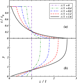
Figure 1: (Color online ) The ratio $\epsilon/\epsilon_{0}$ and flow rapidity $y$ as a function of $z/l$ for different values of $t/l$$\leq$$l/c_{s}$ obtained with the Riemann simple wave solution.

1. For zero rapidity $y$=0 ($v$=0) with the fluid at rest, we have $y$=0 ($\epsilon$=$\epsilon_{0}$) at the spatial coordinate $x$=$-c_{s}t$ (or $z$=$l$-$c_{s}t$).

   The rarefaction wave starts at $z$=$l$ and propagates inward to $z$=0 with the speed of sound $c_{s}$. The rarefaction wave reaches the spatial origin $z$=0 at time $t=l/c_{s}$=$\sqrt{3}l$.

2. As $y$ increases, $\zeta$ becomes more and more negative, and the energy density $\epsilon$ decreases. The variation of $y$ traces out the whole curve of $\epsilon/\epsilon_{0}$ as a function of $z/l$ for a fixed $t$.

3. From Eq. (19), we note that $x$=0 ($z$=$l$) occurs at $\zeta=-c_{s}(\tanh^{-1}c_{s})$, for different times $t$. Thus the curves of $\epsilon/\epsilon_{0}$ for different $t$ meet at the same point of $\epsilon/\epsilon_{0}=\exp\{-4c_{s}(\tanh^{-1}c_{s})\}\sim 0.22$ in Fig. 1.

4. The fluid expands outward and the velocity of the fluid element increases as the fluid coordinate increases. The farthermost reach of the fluid element occurs at $y$$\to$$\infty$, ($v$$\to$1 and $x$$\sim$$t$), which corresponds to $z$$\sim$$(l+t$). The velocities of the fluid elements in contact with the vacuum approach to, and are limited by, the speed of light.

V Hydrodynamic evolution after $t\geq l/c_{s}$

After the time $t$$\geq$$l/c_{s}$, the rarefaction wave that starts from the edge of the slab at $z$=$l$ reaches the center of the slab at $z$=0 (Fig. 1). Subsequent expansion of the fluid in the central region will proceed through the Khalatnikov solution of Eqs. (5), (6), and (8). To determine $(\zeta,y)$ as a function of $(z,t)$, it is useful to express the derivatives of $\chi(\zeta,y)$ explicitly in terms of $\zeta$ and $y$ so that Eqs. (5) and (6) for the coordinates $(x,t)$ are explicit functions of $(\zeta,y)$. The quantities $(\zeta,y)$ can then be inverted to become a function of $(x,t)$.

Using Eq. (8), we can take the derivative with respect to $\zeta$ and we get

$$\frac{\partial\chi}{\partial\zeta}(\zeta,y) = \chi+l\sqrt{3}e^{-\zeta}I_{0}\left[\sqrt{\zeta^{2}-\frac{1}{3}y^{2}}\right].$$ (20)

We take the derivative of $\chi$ with respect to $y$ and we get two terms,

$$\frac{\partial\chi}{\partial y} = -l\sqrt{3}e^{\zeta}\int_{y/\sqrt{3}}^{-\zeta}e^{2\zeta^{\prime}}\frac{\partial}{\partial y}I_{0}\left[\sqrt{\zeta^{\prime 2}-\frac{1}{3}y^{2}}\right]d\zeta^{\prime}+{\cal I},$$

where $\cal I$ is the derivative with respect only to the lower limit $y/\sqrt{3}$. We also have $I_{0}^{\prime}(x)=I_{1}(x)$ Abr65 , and thus

$$\frac{\partial\chi}{\partial y} = l(y/\sqrt{3})e^{\zeta}\int_{y/\sqrt{3}}^{-\zeta}e^{2\zeta^{\prime}}\frac{I_{1}\left[\sqrt{\zeta^{\prime 2}-\frac{1}{3}y^{2}}\right]}{{\sqrt{\zeta^{\prime 2}-\frac{1}{3}y^{2}}}}d\zeta^{\prime}+{\cal I}.$$

We can evaluate ${\cal I}$ to yield

$${\cal I} = le^{\zeta}e^{2y/\sqrt{3}}.$$ (21)

Adding these two terms, we have

$$\frac{\partial\chi}{\partial y}(\zeta,y) = l(y/\sqrt{3})e^{\zeta}\int_{y/\sqrt{3}}^{-\zeta}e^{2\zeta^{\prime}}\frac{I_{1}\left[\sqrt{\zeta^{\prime 2}-\frac{1}{3}y^{2}}\right]}{{\sqrt{\zeta^{\prime 2}-\frac{1}{3}y^{2}}}}d\zeta^{\prime}$$ (22)

$$+le^{\zeta}e^{2y/\sqrt{3}}.$$

With the knowledge of $\partial\chi/\partial\zeta$ and $\partial\chi/\partial y$ given by Eqs. (20) and (22), the right-hand sides of Eqs. (5) and (6) give $(x,t)$ as explicit functions of $(\zeta,y)$. The integral in Eq. (22) can be evaluated numerically as the limits of the integration and the integrands are known functions of $\zeta$ and $y$.

The hydrodynamical description is simplest if we succeed in expressing $(\zeta,y)$ as a function of $(z,t)$. For this purpose, it is necessary to invert Eqs. (5) and (6) from $(z,t)$(function of $\zeta,y$) to $(\zeta,y)$(function of $z,t$). We consider a fixed value of $t$, and we increase stepwise the value of $y$, starting from zero. For each pair values of $(t,y)$, Eq. (5) presents itself as an equation for the unknown quantity $\zeta$ (or equivalently, $\epsilon/\epsilon_{0}$). We can solve this Eq. (5) with only one unknown $\zeta$ by the Newton’s method using a good guessed value of $\zeta$, starting at $y=0$. From Eqs. (20) and (5), a good guess on the value of $\zeta$ for a given $t$ and $y$=0 is

$$\zeta^{(0)} = -\frac{1}{2}\ln\left(\frac{t}{\sqrt{3}l}\right).$$ (23)

Subsequent guesses can then be obtained using Newton’s method after numerically evaluating the change in the residue as a function of a small change in $\zeta$. Newton’s method has a rapid convergence. After the solution for $\zeta$ is obtained, Eqs. (20) and (22) are then used with Eq. (6) to calculate the value of $x$. The newly determined $\zeta$ can be used as the guess for the next $y$ to get the new solution of $\zeta$.

VI Khalatnikov solution and Matching to the Simple Wave solution for $t\geq l/c_{s}$

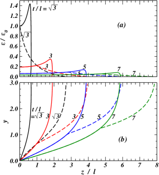
Figure 2: (Color online ) The quantities $(\epsilon/\epsilon_{0},y)$ as a function of $z/l$ for different values of $t/l$. The solid curves give the Khalatnikov solution which must be matched on to Riemann simple wave solutions at the edge boundaries shown as dashed curves. A complete hydrodynamical solution consists of the Khalatnikov solution for small $z/l$ (solid curve) joining on to the matched Riemann solution for large $z/l$ (dashed curve).

The Khalatnikov solution is not applicable before the time coordinate $t<l/c_{s}$. At $t$=$l/c_{s}$=$\sqrt{3}l$, the rarefaction wave has just reached the center of the slab at $z=0$ and the fluid motion described by the Khalatnikov solution has just started to become applicable. We show in Fig. 2 the Khalatnikov solution for $t/l$=1/$c_{s}$, 3, 5, and 7 as a function of $z/l$ as solid curves. At $t$=$l/c_{s}$, the Khalatnikov solution has an energy density exceeding the initial density and increasing as a function of $z$. It decreases precipitously at $z/l$$\sim$0.7 . At subsequent time coordinates, the energy density rises as a function of $z$ and decreases precipitously near $t$$\sim$$(z-l)$. The corresponding rapidity increases monotonically and rapidly as a function of increasing $z/l$

However, not all portions of the Khalatnikov solution shown as the solid curves can be used to describe the evolution of the system because the dynamics at the edge region is described by the propagation of a disturbance arising from the presence of the edge boundary. The accompanying hydrodynamical motion in the edge region is a Riemann simple wave propagating from the edge toward the center. The hydrodynamical solution at the edge of the slab is governed by the Riemann simple wave solution. The Khalatnikov solution that is applicable in the interior of the slab needs to be matched on and switched to the simple wave solution when the energy density logarithm $y$ matches the rapidity $y$ by Eq. (14), $y=-\zeta/c_{s}$. For $t\geq l/c_{s}$, the complete hydrodynamical solution for the fluid with the Landau initial condition consists of the Khalatnikov solution in the interior region of small $|z|$, and the matched Riemann simple wave solution at the edge boundaries of the system.

We can carry out the matching in the following way. We study the Khalatnikov solution for a fixed value of $t$ ($\geq$$l/c_{s}$) and increase stepwise the value of $y$, starting from $y$ =0. We calculate $\zeta$, $x$, and $z$ as a function of $t$ and $y$, using the method outlined in the last section. After determining $\zeta$ for the pair of $(t,y)$ values, we test whether $-\zeta/c_{s}$=$-\sqrt{3}\zeta$ remains greater than $y$ or not. If $-\sqrt{3}\zeta$ remains greater than $y$, we proceed to the next incremented value of $y$ and look for the Khalatnikov solution for the next set of $(t,y)$ pair. On the other hand, when $-\sqrt{3}\zeta$ is equal to or just begin to be greater than $y$, the hydrodynamical solution will be switched from the Khalatnikov solution to the Riemann simple wave solution for subsequent $y$ values.

For the Riemann simple wave solution in the boundary region for a fixed value of $t$, we increase stepwise the value of $y$. The energy density logarithm variable $\zeta$ is then given by $\zeta=-c_{s}y$. Knowing and the values of $t$, $y$ and $\zeta$, the spatial coordinate $x$ is given by Eq. (19). This stepwise increase of $y$ allows us to trace the energy density as a function of the longitudinal coordinates.

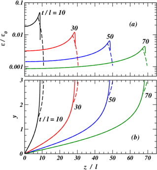
Figure 3: (Color online ) The quantities $(\epsilon/\epsilon_{0},y)$ as a function of $z/l$ for different values of $t/l$. The solid curves give the Khalatnikov solutions which must be matched on to Riemann simple wave solutions shown as dashed curves. A complete hydrodynamical solution consists of the Khalatnikov solution for small $z/l$ (solid curve) joining on to the matched Riemann solution for large $z/l$ (dashed curve).

At $t$=$l/c_{s}$=$\sqrt{3}l$, the matching of the Khalatnikov solution with the Riemann simple wave solution occurs at $z=0$. Thus the solid curve of the Khalatnikov solution is not applicable at $t=\sqrt{3}l$. In its place as the solution of Landau hydrodynamics is the Riemann simple wave solution starting from $z=0$ shown as the dashed curve in Fig. 2. Therefore, at $t$=$l/c_{s}$=$\sqrt{3}l$, even though the Khalatnikov solution begins to emerge, it does not contribute to the hydrodynamical solution with the Landau initial condition.

At higher values of $t$, the fluid expands outward and the longitudinal region under the Khalatnikov solution begins to expand. At $t$=3$l$, the Khalatnikov solution extends to $z$$\sim$$l$ where the matching with the Riemann simple wave solution occurs. At $t=5l$, the Khalatnikov solution extends farther out to $z$$\sim$$3l$ where the matching occurs. The extension of the longitudinal region under the Khalatnikov solution increases approximately linearly with time $t$. On the other hand, the extension of the Riemann simple wave solution spans a longitudinal length of order $3l$ and is approximately independent of $t$. Thus, the Khalatnikov solution covers a longitudinal region less than the Riemann waves for $t\lesssim 5l$, but a longitudinal region greater than the Riemann waves for $t\gtrsim 5l$. The full hydrodynamical solution consists of the Khalatnikov solution in the region of small $z$ (solid curves) and the matched Riemann simple waves solution in the region of large $z$ (dashed curves) in Fig. 2. They are the hydrodynamical solutions satisfying the boundary conditions.

We show in Fig. 3 the Khalatnikov solutions as solid curves for $t/l$=10, 30, 50, and 70. The Riemann simple wave solutions which match with the Khalatnikov solutions are given as dashed curves. At $t$=10$l$, the Khalatnikov solution extends to $7.5l$ and the simple wave solution extends over a length of about $3l$. At later times when $t\gg l$, the matching occurs at a spatial coordinate just a few units less than $t$ with a simple wave that is approximately $3l$ in length. As the simple wave region extends approximately to only a few units of $l$ and $t\gg l$, the simple wave region is much smaller than the Khalatnikov solution region for large values of $t$.

VII Hydrodynamical solution in ($\tau$, $y_{s}$)

To study the question of boost invariance, it is useful to introduce $\tau$ and $y_{s}$ which are related to $(t,z)$ by

$$\tau =\sqrt{t^{2}-z^{2}}=\sqrt{t^{2}-(x+l)^{2}},$$ (24a)

$$y_{s} =\frac{1}{2}\ln\frac{t+z}{t-z},$$ (24b)

$$z =x+l.$$ (24c)

The inverse relations are

$$t=\tau\cosh y_{s},$$ (25a)

$$z=x+l=\tau\sinh y_{s}.$$ (25b)

Strictly speaking, only for solutions that are boost-invariant with respect to the origin at $(t,z)$=0 can the quantity $\tau$ be properly called the proper time and $y_{s}$ the associated spatial rapidity. As we do not possess a boost-invariant initial condition, the coordinates $(\tau,y_{s})$ can only be approximately and analogously identified with the proper time and the spatial rapidity, respectively. Such an approximate identification allows their use as tools to judge the degree of boost invariance of a hydrodynamical evolution. Specifically, at a constant value of $\tau$, a boost-invariant hydrodynamical evolution will be indicated by an energy density $\epsilon$ that is independent of $y_{s}$ and a flow rapidity $y$ equal to the spatial rapidity $y_{s}$. Conversely, at a constant value of $\tau$, the deviation of $\epsilon$ from a constant as a function of $y_{s}$ or the inequality of $y$ and $y_{s}$ will be an indication of boost-non-invariance. The degree to which $\tau$ can be approximately identified as the proper time will depend on how close to boost invariance the solution will turn out to be.

With this choice of the $(\tau,y_{s})$ coordinates, only regions with $t$$>$$|z|$ possess real $\tau$ and $y_{s}$ to fall within our realm of description. The limits of real $\tau$ and $y_{s}$ are the straight lines $t$=$\pm z$ for which $\tau$=0. Therefore, at all times $t$, there are boundary edge regions with a finite width $\Delta z$=$l$ in the simple wave regions, for which $|z|$$>$$t$, and $\tau$ and $y_{s}$ are not real. Such small edge boundary regions fall outside our realm of description.

We need to express the Khalatnikov solution and the Riemann solution in terms of $\tau$ and $y_{s}$. We represent $(\tau,y_{s})$ in terms of $(t,x)$ by Eq. (23) which are in turn represented as functions of $\zeta$ and $y$ by Eqs. (5) and (6), with the hydrodynamical potential $\chi$ determined by Eq. (8). With the knowledge of $\partial\chi/\partial\zeta$ and $\partial\chi/\partial y$ given by Eqs. (20) and (22), the $(\tau,y_{s})$ variables are explicit functions of $(\zeta,y)$.

We can express the Riemann simple wave solution as a function of the $(\tau,y_{s})$ coordinates by substituting (25) into (19). We introduce the effective velocity $a$ as

$$x=\tau\sinh y_{s}-l = a\tau\cosh y_{s}=at,$$ (26)

where

$$a=\frac{v-c_{s}}{1-vc_{s}}.$$ (27)

The Riemann simple wave solution in terms of $(\tau,y_{s})$ becomes

$$e^{y_{s}} = \frac{1+\sqrt{1+(\tau/l)^{2}(1-a^{2})}}{(\tau/l)(1-a)},$$ (28)

which describes the hydrodynamical motion of disturbances in the boundary regions of the slab. The Khalatnikov solution needs to match to the Riemann simple wave solution when the energy density logarithm $\zeta$ and the rapidity $y$ are related by the speed of sound as $\zeta=-c_{s}y$ given by Eq. (14).

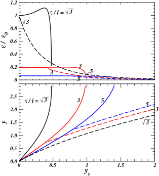
Figure 4: (Color online ) The quantities $(\epsilon/\epsilon_{0},y)$ as a function of the spatial rapidity $y_{s}$ for different values of $\tau/l$. The solid curves give the Khalatnikov solutions which must be matched on to Riemann simple wave solutions shown as dashed curves. A complete hydrodynamical solution consists of the Khalatnikov solution for small $y_{s}$ (solid curve) joining on to the matched Riemann solution for large $y_{s}$ (dashed curve).

We consider a fixed value of $\tau$$\geq$$l/c_{s}$ and stepwise increase the value of $y$, starting from $y$ =0. We can obtain the hydrodynamical description of $(\zeta,y)$ as a function of $(\tau,y_{s})$ by inverting Eq. (24) and its associated equations. For each pair of $(\tau,y)$ values, equation (24a) together with the associated supplementary equations (5) and (6) presents itself as an equation for the unknown quantity $\zeta$. We can solve this equation with only one unknown $\zeta$ by Newton’s method using a satisfactory guessed value of $\zeta$, starting at $y$=0. From Eqs. (20) and (5), a good guess (trial value) for the value of $\zeta$ at $y$ =0 for a given $\tau$ is

$$\zeta^{(0)} = -\frac{1}{2}\ln\left(\frac{\tau}{\sqrt{3}l}\right).$$ (29)

After the solution of $\zeta$ is obtained, Eqs. (20) and (22) are then used with Eq. (6) to calculate the value of $x$, $z$ and $y_{s}$. The newly determined $\zeta$ can be used as the trial value for the next $y$ to get the new solution of $\zeta$.

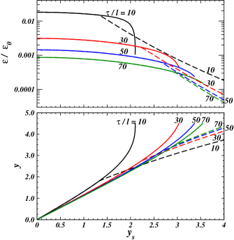
Figure 5: (Color online ) The quantities $(\epsilon/\epsilon_{0},y)$ as a function of the spatial rapidity $y_{s}$ for different values of $\tau/l$. The solid curves give the Khalatnikov solutions which must be matched on and switched to the Riemann simple wave solutions shown as dashed curves.

Using the method we have just outlined for $\tau$$\geq$$l/c_{s}$, we can determine the Khalatnikov solution as a function of the spatial rapidity $y_{s}$ for a fixed value of $\tau$ shown as solid curves in Fig. 4. In the time domain of Fig. 4, $((\epsilon/\epsilon_{0})$ is relatively flat as a function of $y_{s}$ but the flow rapidity $y$ is consistently greater than $y_{s}$ except at very large values of $y_{s}$. However, not all parts of the Khalatnikov solution can be used for our complete hydrodynamical solution. It is necessary to match the Khalatnikov solution to the Riemann simple wave when $\zeta$ is equal to $-c_{s}y$.

We carry out the simple wave matching of the Khalatnikov solution by testing $-\zeta$ against $c_{s}y$. When $-\zeta$ is equal to or just begin to be greater than $c_{s}y$, the solution will be switched to the Riemann simple wave solution for subsequent $y$ values. For this Riemann simple wave solution, the energy density logarithm variable $\zeta$ is given by $\zeta=-c_{s}y$ and the spatial rapidity $y_{s}$ is given by Eq. (28). The complete hydrodynamical solution consists of the Khalatnikov solution in the region of small $y_{s}$ (solid curves) and the matched Riemann simple waves solution in the region of large $y_{s}$ (dashed curves) in Fig. 4.

We show in Fig. 5 the dynamics of the system for later times of $\tau=10$ 30, 50, and 70 $l$. In this time domain, the energy density in the region of small $y_{s}$ decreases as a function of $y_{s}$. For example, for $\tau/l$=70, $(\epsilon/\epsilon_{0})$ decreases by a factor of three as $y_{s}$ increases from 0 to 3, indicating a lack of boost invariance for this value of $\tau$. The flow rapidity $y$ is slightly greater than the spatial rapidity $y_{s}$.

VIII Other comparisons

The solution of $(\zeta,y)$ as a function of $(t,z)$ or $(\tau,y_{s})$ allows one to extract other hydrodynamical quantity of interest. In addition to the energy density, one can calculate the spatial profiles of the temperature or entropy density at different times $t$ or proper times $\tau$.

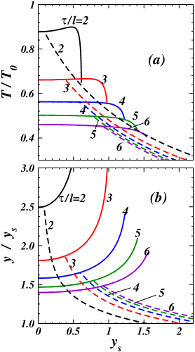
Figure 6: (Color online ) The quantities $T/T_{0}$ and $y/y_{s}$ as a function of $y_{s}$ for different values of the $\tau/l$. The solid curves give the Khalatnikov solutions for small $y_{s}$ which must be matched on and switched to the Riemann simple wave solutions for large $y_{s}$ shown as dashed curves.

We show the ratio $T/T_{0}$ in Fig. 6a, and the ratio $y/y_{s}$ in Fig. 6b, as a function of $y_{s}$ for different values of the proper time $\tau/l$. We observe that for small values of $\tau/l$= 2-6, the Khalatnikov solution starts to emerge from the central region, the longitudinal length of the Khalatnikov solution included into the hydrodynamical description gradually increases. In this time domain, the temperature or the energy density of the Khalatnikov solution is relatively flat as a function of $y_{s}$, but the ratio $y/y_{s}$ is consistently greater than unity, which indicates a high degree of boost-non-invariance, especially during the early stage of the hydrodynamical evolution.

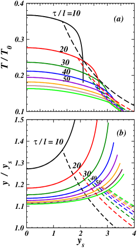
Figure 7: (Color online ) The quantities $T/T_{0}$ and $y/y_{s}$ as a function of $\tau/l$ for different values of the spatial rapidity $y_{s}$. The solid curves give the Khalatnikov solutions for small $y_{s}$ which must be matched on to Riemann simple wave solutions for large $y_{s}$ shown as dashed curves.

Fig. 7 gives $T/T_{0}$ and $y/y_{s}$ as a function of $y_{s}$ for different $\tau/l$=10, 20, 30, 40, and 50. We observe that the temperature decreases gradually as a function of the spatial rapidity $y_{s}$, and the ratio of $y/y_{s}$ is consistently greater than unity, even for $\tau$$\sim$ 80$l$.

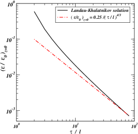
Figure 8: (Color online ) The ratio $\epsilon/\epsilon_{0}$ at $z$=0 ($y_{s}$=0) as a function of $\tau/l$. The solid curves represent the solutions from the Khalatnikov solution with the Landau initial condition, and the dashed curve is the behavior expected from Bjorken hydrodynamics.

In Fig. 8, we show the ratio $\epsilon/\epsilon_{0}$ at the center of the slab at $z$=0 as a function of the $\tau/l$. The energy density decreases with $\tau/l$ but the decrease does not follow the Bjorken limit of $\epsilon/\epsilon_{0}\propto 1/\tau^{4/3}$. Bjorken-like behavior of $\epsilon/\epsilon_{0}\propto 1/\tau^{4/3}$ behavior occurs only at the very late stage of $\tau/l\sim$ 80.

The relation between $\epsilon/\epsilon_{0}$ and $\tau/l$ at $z$=0 ($y_{s}$=0) in Fig. 8 can be fitted very well by the empirical formula

$$\frac{\epsilon}{\epsilon_{0}}\simeq b\left(\frac{\tau}{l}\right)^{-\frac{4}{3}+a\frac{l}{\tau}+c\left(\frac{l}{\tau}\right)^{d}}$$ (30)

where, respectively, $a\simeq 2.60,b\simeq 0.213,c\simeq 2.25,d\simeq 3.48$. This above formula can be used to provide an effective correction to the equivalent Bjorken energy formula

$$\frac{\epsilon}{\epsilon_{0}}=b^{\prime}\left(\frac{\tau}{l}\right)^{-4/3}$$ (31)

that is usually used to estimate the initial energy density given the initial time $\tau_{0}$ and the experimentally observed energy density $dE/dy$, which, for a rapidity-independent system is

$$\epsilon=\frac{1}{S\tau_{0}}\frac{dE}{dy},$$ (32)

where $S$ is the transverse area of the system. Since the Landau model does not require full stopping but just lack of transparency (see the introduction in Sen14 ), the initial energy density compatible with the Landau model is not necessarily $\sqrt{s}N_{part}$ (which, at ultra-relativistic energies is too high). The initial energy density assuming a Landau initial condition can instead be estimated from Eqs. (30) and (32) scaled by $y_{s}/y$, given an estimate of the initial time $\tau_{0}$ of the system.

Similarly, Fig. 7 is well-described at $z$=0 ($y_{s}$=0), also in the asymptotic limit $\lim_{\tau\rightarrow\infty}y/y_{s}$=1, by this parametrization

$$\frac{y}{y_{s}}\simeq 1+a\left(\frac{l}{\tau}\right)^{b}+c\left(\frac{l}{\tau}\right)^{d},$$ (33)

where $a=1.942,b=1.178,c=0.220,d=0.184$. This parametrization can be used to obtain a back-of-the-envelope estimate of the goodness of the Bjorken approximation, assuming Landau initial conditions and a given initial time $\tau_{0}$ that is approximately related to the initial slab width by $\tau_{0}\sim l$.

Transverse expansion will of course alter these approximation to $\mathcal{O}(50\%)$, but for that a realistic numerical calculation such as Sen14 is required.

IX Conclusions and Discussions

We undertake our present review to rectify three technical gaps that hinders the application of the analytical solutions of Landau hydrodynamics. First, we show that the earliest history can be described exclusively by the Riemann simple wave solution. Secondly, the inversion of the Khalatnikov solution can be carried out successfully with well-outlined procedures. Thirdly, we show how the Khalatnikov solution and the Riemann simple wave solution can be matched at different time domains. In consequence, the analytical Khalatnikov solution and the matched Riemann simple wave solution provide a complete picture of the full evolution of the relativistic hydrodynamics of a (1+1)-dimensional system. Our examination with the Landau initial condition reveals that the Riemann simple wave solutions are always present at the two edge boundaries of the slab, and the Khalatnikov solution properly appears only after the time coordinate $t$$\geq$$l/c_{s}$.

The evolution can be depicted as following three stages of development. In the first stage of $t$$\leq$$l/c_{s}$, a Riemann simple wave (rarefaction wave) moves towards the center and depletes the density near the central region. One edge of the simple wave reaches the center of the slab at $t$=$l/c_{s}$. The other edge expands the matter into the vacuum. In the edge region of matter expansion, the velocity increases with the distance from the center, and the matter always approaches the speed of light as it comes in contact with the vacuum. In this first stage, the Riemann simple wave solution suffices to describe the hydrodynamical evolution.

At the second stage of $\sim$$5l/c_{s}$$\gtrsim$$t$$\geq$$l/c_{s}$, the interior region begins to expand, and both the Riemann solution and the Khalatnikov solution occupy comparable longitudinal regions and must be used simultaneously in different longitudinal regions to describe the hydrodynamical evolution. Such a situation arises because the Khalatnikov solution describes only the hydrodynamical evolution of the system in the interior region whereas the dynamics at the edge is described by the propagation of a disturbance arising from the presence of the boundary edge. The accompanying hydrodynamical motion is a Riemann simple wave propagating from the edge boundary toward the center. The longitudinal length of the hydrodynamical motion governed by the Khalatnikov solution and the Riemann simple wave solution depends on the time in the Khalatnikov solution expansion, $t-l/c_{s}$. The greater is the time $t-l/c_{s}$ compared to the Riemann simple wave characteristic time $\sim 2l/c_{s}$, the greater is the spatial region governed by the Khalatnikov solution.

In the third stage when $t$$\gtrsim$$(\sim$$6l/c_{s}$), the hydrodynamical motion is dominated by the Khalatnikov solution, with the simple waves occupying only a relatively small longitudinal region at the boundary edges. The Khalatnikov solution suffices approximately for the description of the hydrodynamics of the system, if the edge boundary region can be neglected. While the Khalatnikov and the simple wave interplay at different stages of the hydrodynamical evolution, Belenkij and Landau showed that entropy of the system is concentrated in the central region while total energy (including both internal and kinetic energies and as seen in the laboratory frame) is concentrated in the boundary region Bel56 .

As hydrodynamics gains in importance in high-energy heavy-ion collisions, the method of extracting the analytical solutions presented here may be useful for those who would like to use the procedure to examine the approximate behavior of a relativistic system undergoing a one-dimensional expansion. In fact, as shown earlier by Rischke and Gyulassy Ris96 ; Ris96a , the main features of the hydrodynamics of (2+1)- and (3+1)-dimensional relativistic hydrodynamics contains many features similar to the (1+1)-dimensional system. An explicit outline presented here on how the different analytical solutions interplay in a completely analytical treatment enhances our understanding of the hydrodynamical evolution process.

With regard to the question of the comparison of Landau hydrodynamics and Hwa-Bjorken boost-invariance hydrodynamics Hwa74 ; Bjo83 , we note that boost invariance implies that not only is the energy density independent of $y_{s}$, the flow rapidity $y$ should also coincide with the spatial rapidity $y_{s}$. As shown previously in Landau (1+1)-dimensional hydrodynamics in Sri92 and in numerically-intensive event-by-event (3+1)-dimensional hydrodynamics with supercomputers Sen14 , the Landau initial condition does not possess boost invariance and during the Landau hydrodynamical evolution the flow rapidity does not equal the spatial rapidity even at late times. The approach to boost-invariance appears to be a slow process, even though the energy density or temperature appears to be relatively flat as a function of $y_{s}$ Sen14 .

This research used resources of the Oak Ridge Leadership Computing Facility at the Oak Ridge National Laboratory, which is supported by the Office of Science of the U.S. Department of Energy under Contract No. DE-AC05-00OR22725. GT also acknowledges support from DOE under Grant No. DE-FG02-93ER40764.

Appendix A Generalization of the analytical solutions of Landau hydrodynamics for different $c_{s}$

For completeness, we summarize below the analytical solutions of Landau hydrodynamics and the dependencies on the speed of sound $c_{s}$. We consider an equation of state

$$p=c_{s}^{2}\epsilon,$$ (34)

where $c_{s}$ is assumed to be a constant. The relations between the energy density, entropy density, and the temperature in Eqs. (1)-(3) are modified to be

$$\zeta = \ln(T/T_{0})=\frac{c_{s}^{2}}{1+c_{s}^{2}}\ln(\epsilon/\epsilon_{0}),$$ (35)

$$\epsilon/\epsilon_{0} = (T/T_{0})^{1+1/c_{s}^{2}}=e^{\zeta(1+c_{s}^{2})/c_{s}^{2}},$$ (36)

$$s/s_{0} = (\epsilon/\epsilon_{0})^{1/(1+c_{s}^{2})}=(T/T_{0})^{1/c_{s}^{2}}=e^{\zeta/c_{s}^{2}}.$$ (37)

The space-time coordinates $(t,x)$ are related to $(\zeta,y)$ and the hydrodynamical potential $\chi$ as in Eqs. (5) and (6). When the speed of sound $c_{s}$ is taken into account, the Khalatnikov solution, Eq. (8), is modified to be Beu08

$$\chi(\zeta,y)\!=\!-\frac{le^{\zeta}}{c_{s}}\!\!\int^{-\zeta}_{c_{s}y}\!\!e^{\frac{c_{s}^{2}+1}{2c_{s}^{2}}\zeta^{\prime}}\!I_{0}\!\left(\frac{1-c_{s}^{2}}{2c_{s}^{2}}\sqrt{\zeta^{\prime 2}-{c_{s}^{2}y^{2}}}\right)\!d\zeta^{\prime}.~{}~{}~{}~{}~{}~{}$$ (38)

The Riemann solution as a function of the speed of sound $c_{s}$ is already given by Eqs. (14) and (19).

References

- (1) L. D. Landau, Izod. Akad. Nauk SSSR 17, 51 (1953).
- (2) S. Z. Belenkij and L. D. Landau, Usp. Fiz. Nauk 56, 309 (1955).
- (3) S. Z. Belenkij and L. D. Landau, Nuovo Cimento, Suppl. 3, 15 (1956).
- (4) S. Z. Belenkij and L. D. Landau, in Collected Papers of L. D. Landau, Edited by D. Ter Haar, Gordon and Breach, New York, 1965, page 569.
- (5) I. M. Khalatnikov, Zh. Eksp. Teor. Fiz. 27, 529 (1954).
- (6) L. D. Landau and E. M. Lifshitz, Fluid mechanics, Pergamon Press, 1958.
- (7) S. Z. Belenkij and G. A. Milekhin, Zh. Eksp. Teor. Fiz. 29, 20 (1956) [Sov. Phys. JETP 2, 14 (1956)].
- (8) G. A. Milekhin, Zh. Eksp. Teor. Fiz. 35, 978 (1958) [Sov. Phys. JETP 8, 682 (1959)].
- (9) G. A. Milekhin, Zh. Eksp. Teor. Fiz. 35, 1185 (1958) [Sov. Phys. JETP 8, 829 (1959)].
- (10) I. L. Rosental, Zh. Eksp. Teor. Fiz. 31, 278 (1957) [Sov. Phys. JETP 4, 217 (1959)].
- (11) S. Amai, H. Fukuda, C. Iso, and M. Sato, Prog. Theo. Phys. 17, 241 (1957).
- (12) P. Carruthers and Minh Doung-van, Phys. Rev. D 8, 859 (1973).
- (13) P. Carruthers, “Heretical Models of Particle Production”, Ann. N. Y. Acad. Sci. 229, 91 (1974).
- (14) F. Cooper and G. Frye, Phys. Rev. D 10, 186 (1974).
- (15) F. Cooper, G. Frye, and E. Schonberg, Phys. Rev. D 11, 192 (1975).
- (16) M. I. Gorenshtein and Yu. M. Sinyukov, Yad. Fiz. 41, 797 (1985) [ Sov. J. Nucl. Phys. 41, 508 (1985)].
- (17) S. Chadha, C. S. Lam, and Y. C. Leung, Phys. Rev. D 10, 2817 (1974).
- (18) D. K. Srivastava, J. Alam, B. Sinha, Phys. Lett. B 296, 11 (1992); D. K. Srivastava, Jan-e Alam, S. Chakrabarty, B. Sinha, S. Raha, Ann. Phys. 228, 104 (1993); D. K. Srivastava, J. Alam, S. Chakrabarty, S. Raha, B. Sinha, Phys. Lett. B 278, 225 (1992).
- (19) S. Paiva, Y. Hama, and T. Kodama, Phys. Rev C55, 1455 (1997).
- (20) B. Mohanty, and Jan-e Alam, Phys. Rev. C 68, 064903 (2003).
- (21) Y. Hama, T. Kodama, O. Socolowski Jr., Braz. J. Phys. 35, 24 (2005); C. E. Aguiar, T. Kodama, T. Osada, Y. Hama, J. Phys. G 27, 75 (2001).
- (22) S. Pratt, Phys. Rev. C 75, 024907 (2007).
- (23) A. Bialas, R. A. Janik, and R. Peschanski, Phys. Rev. C 76, 054901 (2007).
- (24) T. Csörgö, M. I. Nagy, and M. Csanád, Phys. Lett. B 663, 306 (2008).
- (25) G. Beuf, R. Peschanski, and E. N. Saridakis, Phys. Rev. C78, 064909 (2008).
- (26) R. Peschanski and E. N. Saridakis, Nucl. Phys. A849, 147 (2011).
- (27) A. Bialas and R. Peschanski, Phys. Rev. 83, 054905 (2011).
- (28) T. Osada and G. Wilk, Cent. Eur. J. Phys. 7(3), 432 (2009); T. Osada and G. Wilk, Phys. Rev. C77, 044903 (2008).
- (29) E. K. G. Sarkisyan, A.S. Sakharov, AIP Conf. Proc. 828, 35 (2006); E. K. G. Sarkisyan, A.S. Sakharov, [hep-ph/0410324]; E.K.G. Sarkisyan, A.S. Sakharov, Eur. Phys. J. C70, 533 (2010); A.N. Mishra, R. Sahoo, E.K.G. Sarkisyan, A.S. Sakharov, arXiv:1405.2819.
- (30) L. P. Csernai, Soviet Phys. JETP 65, 216 (1987).
- (31) V. K. Magas, L. P. Csernai, and D. D. Strottman, Phys. Rev. C 64, 014901 (2001); V. K. Magas, L. P. Csernai, and D. D. Strottman, Nucl. Phys. A 712, 167 (2002).
- (32) V. K. Magas, L. P. Csernai, E. Molnar, A. Nyiri, and K. Tamosiunas, Eur. Phys. J. A 25, 65 (2005).
- (33) D. H. Rischke and M. Gyulassy, Nucl. Phys. A597, 701 (1996).
- (34) D. H. Rischke and M. Gyulassy, Nucl. Phys. A608, 479 (1996).
- (35) G. Baym, B. Friman, J.-P. Balizot, M. Soyeur, and W. Czyz, Nucl. Phys. A407, 541 (1983).
- (36) Y. Hama and F. W. Pottag, Rev. Bras. Fis. 15, 289 (1985).
- (37) J. Y. Ollitrault, Phys. Rev. D 46, 229, (1992); J. Y. Ollitrault, Eur. J. Phys. 29, 275 (2008).
- (38) L. P. Csernai, Introduction to Relativistic Heavy-Ion Collisions, Willey, 1994; D. Teaney, Phys. Rev. C68, 034913 (2004); T. Hirano and Y. Nara, Nucl. Phys. A743, 395 (2004); P. F. Kolb and U. Heinz,nucl-th/0305084(2003); P. Huovinen and P. V. Ruuskanen, Ann. Rev. Nucl. Par. Sci. (2006); C. Nonaka and B. A. Bass, Phys. Rev. C75, 014902 (2007); O. J. Socolowski, F. Grassi, Y. Hama, and T. Kodama, Phys. Rev. Lett. 93, 182903 (2004); W. N. Zhang, M. J. Efaaf, and C. Y. Wong, Phys. Rev. C70, 024903 (2004); T. Csorgo, F. Grassi, Y. Hama, and T. Kodama, Phys. Lett. 565, 107 (2003); T. Csorgo , Phys. Lett. B663, 306 (2008); C. Y. Wong, Phys. Rev. C78, 054902 (2008); R. Peschanski and E. N. Saridakis, Phys. Rev. C80, 024907 (2009); C. Y. Wong, Introduction to High-Energy Heavy-Ion Collisions, World Scientific Publisher, 1994.
- (39) A. Sen, J. Gerhard, G. Torrieri, K. Read, C. Y. Wong, arxiv: 1403.7990.
- (40) M. Abramowitz and I. Stegun, Handbook of Mathematical Functions, Dover Publications, New York, 1965
- (41) R. C. Hwa, Phys. Rev. D10, 2260 (1974).
- (42) J. D. Bjorken, Phys. Rev. 27, 140 (1983).