Computer Assisted ‘Proof’ of the Global Existence of Periodic Orbits in the Rössler System

Abstract

The numerical optimized shooting method for finding periodic orbits in nonlinear dynamical systems was employed to determine the existence of periodic orbits in the well-known Rössler system. By optimizing the period $T$ and the three system parameters, $a$, $b$ and $c$, simultaneously, it was found that, for any initial condition $(x_{0},y_{0},z_{0})\in\Re^{3}$, there exists at least one set of optimized parameters corresponding to a periodic orbit passing through $(x_{0},y_{0},z_{0})$. After a discussion of this result it was concluded that its analytical proof may present an interesting new mathematical challenge.

1 Introduction

The three-dimensional Rössler system (RS) was originally conceived as a simple prototype for studying chaos [1]. With only one nonlinear term it can be thought of as a simplification of the well-known Lorenz system [2] and as a minimal model for continuous-time chaos [3].

Over the past 38 years the RS has been studied extensively, both in its own right [4, 5, 6, 7, 8, 9, 10, 11, 12, 13, 14, 15] and as a model, to illustrate various nonlinear phenomena and different types of chaos [16, 17, 18, 19]. Surprisingly, despite the literally thousands of scientific articles that have been devoted to the RS, it still poses several open questions. For example, although the conjecture by Leonov [20], about the Lyapunov dimension of the RS (and two other types of Rössler systems), has recently been verified numerically [21], the exact Lyapunov dimension for the RS is not known analytically. Leonov [22] has recently also provided an analytical estimate of the attractor dimension in the RS, however, similar estimates for slightly more general Rössler systems remain a difficult open problem. There is also an ongoing discussion about whether or not the RS can indeed produce a strange attractor, in the same sense as that of the Lorenz system [23, 19].

More pertinent to the present study are the recent articles on the existence or non-existence and/or classification of the periodic orbits of the RS, in terms of its three control parameters $a$, $b$ and and $c$. Starkov and Starkov [24] have shown that, when the parameters satisfy the condition $c^{2}-4ab<0$, no periodic solutions can exist. They have also proved that, when $ac<0$ ($ac>0$) and $ab>0$, the periodic orbits exist entirely in the negative (positive) half space, i.e. $z<0$ ($z>0$).

There have been several attempts to demonstrate the existence of orbits more generally; such as those by Genesio and Ghilardi [25], in which the existence of the quasi-periodic orbits in third-order systems like those of Rössler, Lorenz and Chua et al. [26] are proved. More recently, instead of the focus of such studies being on the unstable orbits, the experimentally observable chaotic and stable periodic orbits of simple chaotic flows, including the RS, have been classified very generally in terms of their control parameters [18]. In the parameter space, families of stable periodic solutions have been found to self-organize about the so-called isolated periodicity hubs of the RS. (See Ref. [18] and the references therein.)

Another active area of related research is on the integrability of the RS [28, 6, 27, 11, 14, 15]. In Ref. [6] it was shown that Darboux integrability of the RS for various parameter values leads to surfaces in state space containing periodic orbits. The bifurcations and routes to chaos in the RS have also been investigated [4, 29] and there is at least one exhaustive study on the complete parametric evolution of the system [12]. (Also see Ref. [13] and the references therein.)

The present work developed as a result of using the RS as a test case for our recently-developed numerical technique (called the optimized shooting method) for finding periodic solutions in nonlinear dynamical systems [30]. During the course of testing our method we discovered that it could optimize the system parameters to find at least one periodic orbit for any initial condition. At first this finding was very surprising to us, and we assumed that it was most likely due to a coding error. We therefore tested the codes more thoroughly and also experimented with a variety of different integration schemes and platforms, in order to verify the results independently. After confirming that our numerical results were indeed accurate, we turned to the literature to establish if a similar result had been reported elsewhere for the RS. However, in all of the related literature we found, there appeared to be no explicit proof (or mention) of the result we had obtained. Hence we consider it worthy of a separate brief report.

We are certainly not the first to use numerical computations to ‘prove’, i.e. motivate, the existence of certain analytical properties. Pilarczyk [16], for example, provides a computer assisted ‘proof’ of the existence of a periodic orbit in the RS. Wilczak and Zgliczyński [17] have also made use of a numerical method to ‘prove’ the existence of two period-doubling bifurcations in Rössler’s system, as well as the existence of a branch of period two points connecting them.

The remaining material in this article is organized as follows. In Sec. 2 we provide a brief description of the optimized shooting method. In Sec. 3 we state the main result in the form of a conjecture and describe the procedure that was followed in order to motivate it. Section 4 ends with a short discussion and conclusion.

2 Optimized shooting method

Today there are a variety of numerical methods available for finding the periodic orbits of nonlinear dynamical systems [31]. For the present purpose we make use of the optimized shooting method [30], which originally enabled us to discover the reported new property of the periodic orbits in the RS [1]. Briefly, this method makes use of Levenberg-Marquardt optimization to find the periodic orbits by minimizing a residual (or error function) [32, 33].

To apply the method to the RS, we re-write the system equations as

$$\dot{x}=T\left(-y-z\right),\;\;\;\dot{y}=T\left(x+ay\right),\;\;\;\dot{z}=T\left(b+z\left(x-c\right)\right),$$ (1)

where $T$ is the (as yet) unknown period of the desired solution and the overdot indicates differentiation with respect to the dimensionless time $\tau=t/T$. Since one period corresponds to integration over $\tau$ from zero to one, we define the residual as

$$\mathbf{R}=\left(\mathbf{x}\left(1\right)-\mathbf{x}\left(0\right),\mathbf{x}\left(1+\Delta\tau\right)-\mathbf{x}\left(\Delta\tau\right)),\ldots,\mathbf{x}\left(1+p\Delta\tau\right)-\mathbf{x}\left(p\Delta\tau\right)\right),$$ (2)

where $\Delta\tau$ is a fixed integration step size, $p=0,1,2,\ldots$ and $\mathbf{x}\equiv\left(x,y,z\right)$. The residual is a function of the initial conditions, period, and three system parameters; since it depends on these through solution of Eq. (1). Furthermore, since $\mathbf{x}(\tau)=\mathbf{x}(\tau+1)$ for periodic solutions, it can immediately be seen that such solutions correspond to a vanishing residual, i.e. the periodic solutions are found by optimizing $\mathbf{R}$ to be as close as possible to zero.

3 Results

We state the main result of this work in the form of a conjecture.

Conjecture: For any initial condition $(x_{0},y_{0},z_{0})\in\Re^{3}$, there exists real parameters, $a$, $b$ and $c$, for Eq. (1), such that its solution is periodic.

For initial conditions on plane $z=0$, inspection of Eq. (1) shows that the conjecture is trivially satisfied: for $a=b=c=0$ the solutions are circles, with periods equal to $2\pi$. The analytical proof of the integrability of the system, for this case, is given in Refs. [7] and [11].

Off the $z=0$ plane the validity of the conjecture is established numerically by performing optimization of the four parameters, $T$, $a$, $b$ and $c$, for sets of randomly selected initial conditions. To facilitate the selection of these initial conditions it is convenient to rewrite Eq. (1) in terms of scaled (primed) coordinates, defined by $x=\alpha x^{\prime}$, $y=\alpha y^{\prime}$, and $z=\alpha z^{\prime}$. Here $\alpha\geq 1$ is the scale factor. In terms of the primed coordinates Eq. (1) is given by

$$\dot{x}^{\prime}=T\left(-y^{\prime}-z^{\prime}\right),\;\;\;\dot{y}^{\prime}=T\left(x^{\prime}+ay^{\prime}\right),\;\;\;\dot{z}^{\prime}=T\left(b/\alpha+\alpha z^{\prime}\left(x^{\prime}-c/\alpha\right)\right).$$ (3)

For a given $\alpha$, the procedure for selecting the initial conditions then consisted of generating $100$ distinct random points, within or on the unit sphere. For each initial condition the optimized shooting method was used to find the four parameters that produce a periodic orbit. As an initial guess for the parameters, we chose $(T,a,b,c)=(5,1,1,1)$. Starting from $\alpha=1$, the value of the scale factor was increased, in steps of $1$, up to the maximum value of $100$. This procedure produced a total of $100\times 100$ random initial conditions. All $10^{4}$ initial conditions were successfully optimized, i.e. in each case the magnitude of $\mathbf{R}$ was successfully optimized to be below the set numerical tolerance ($\left|\mathbf{R}\right|<10^{-12}$ in this calculation).

Table 3 lists the optimized parameters for $15$ arbitrarily chosen periodic orbits.

Table 1: Fifteen of the $10^{4}$ periodic orbits found for the Rössler system via the optimized shooting method. The column headings are as follows: $n$ is the orbit number (used to refer to the orbit in the main text), $\alpha$ is the scale parameter introduced in the main text (see Eq. 3), $x^{\prime}_{0}$, $y^{\prime}_{0}$ and $z^{\prime}_{0}$ are the primed coordinates of the randomly selected initial conditions, $T$ is the period, and the last three columns give the optimized system parameters.

$n$	$\alpha$	$x_{0}^{\prime}$	$y_{0}^{\prime}$	$z_{0}^{\prime}$	$T$	$a$	$b$	$c$
1	1	-0.322	0.283	-0.827	6.285	-0.01832876699	-37.861974659	45.448602039
2	1	0.083	0.498	0.756	6.282	0.01659280123	34.3119795334	45.496814976
3	1	0.271	-0.033	-0.492	6.284	-0.01074867143	-22.256338664	45.495734090
4	1	-0.843	-0.154	-0.338	6.283	-0.00756927443	-15.661740755	45.483293583
5	1	0.920	-0.101	-0.062	6.285	-0.00133598606	-2.7619826425	45.463987246
6	10	0.274	-0.843	-0.019	6.280	-0.00346652925	-9.6387456311	53.299901841
7	10	-0.431	0.429	-0.132	6.287	-0.02714795455	-75.519091787	52.954713982
8	10	-0.762	0.094	-0.023	6.283	-0.00504377136	-13.929997631	52.959008822
9	10	0.721	0.212	0.532	6.303	0.09058831072	242.356061832	52.926271854
10	10	0.212	-0.008	-0.946	6.412	-0.18855060455	-483.78516338	53.074125658
11	100	0.370	0.525	-0.489	9.221	-0.72151348243	-2913.5197570	96.641076651
12	100	0.465	-0.177	0.111	6.506	0.27456932042	1.25094211568	35.351207642
13	100	0.045	-0.881	0.206	1.670	0.28422944418	0.06378881294	25.148204118
14	100	0.448	-0.071	0.533	7.016	0.41997047657	5480.91338691	148.08093025
15	100	0.177	-0.786	0.321	3.795	0.35076508274	0.24268923009	27.447807055

For ease of presentation, the randomly chosen initial conditions were first rounded off to three decimal places, before applying the optimized shooting method. Thus the initial conditions, as listed in columns 3-5 of Table 3, are exact. On the other hand the periods listed in column 6 are given approximately to three decimal places. Since they are not required to reconstruct the orbits, their full 11 digit accuracy is not required here.

Two other features of Table 3 are also worth mentioning. First, we notice that the signs of the parameters $a$ and $b$ are always the same as that of $z_{0}^{\prime}$. This is a property of all the found orbits and it confirms the analytical result proved by Starkov and Starkov [24]: when $ac<0$ ($ac>0$) and $ab>0$, the periodic orbits exist entirely in the negative (positive) half space. Second, in Ref. [24] it was also shown that for $c^{2}-4ab<0$, no periodic orbits can exist. In Table 1, and indeed for all the found orbits, $c^{2}-4ab$ is positive. Thus our results are consistent with the known classifications for periodic orbits in the RS.

In total more than 100 spot checks were made on randomly selected orbits taken from the set of $10^{4}$. Such checks were made by plotting and visually inspecting the selected orbits. Figure 1 shows

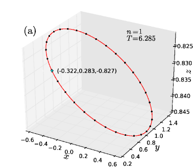
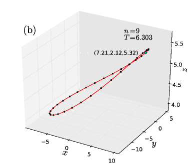
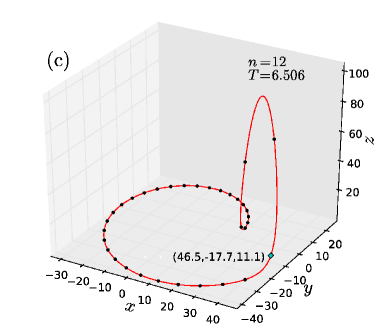
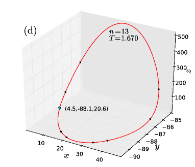
Figure 1: Phase portraits of four arbitrarily selected periodic orbits, chosen from Table 3. The initial condition for each orbit is indicated by a blue square marker. Black filled circular markers indicate points along the orbit, every 200 integration time steps. Since a fixed time step of $\Delta\tau=1/1024$ was used, the circular markers provide an indication of the velocity $(\dot{x}(\tau),\dot{y}(\tau),\dot{z}(\tau))$ along each orbit.

the plots for four orbits that are listed in Table 3, i.e. orbits numbers $1,9,12$ and $13$. In Fig. 1(a) it can be seen that orbit one is confined to lie within the negative half space $\Re^{3}-\{z\geq 0\}$, while orbits 9, 12 and 13, shown in Figs. (b)-(d), occur in the positive half space $\Re^{3}-\{z\leq 0\}$. This observation is consistent with the form of Eq. (1). If periodic orbits existed that crossed from one half space into the other, they would have to intersect the plane $z=0$ more than once. Moreover, at $z=0$ the sign of $\dot{z}$ would have to be positive (negative) in going from the negative (positive) half space to the positive (negative) half space. However, the form of Eq. (1) clearly excludes this possibility, since for $z=0$ the sign of $\dot{z}$ is determined by the parameter $b$. Therefore, for a given set of parameters, the sign of $\dot{z}$ at $z=0$ cannot change. Hence, the non-trivial periodic orbits are confined to lie entirely within one half space or the other.

Finally, as an alternative way (i.e. without using the residual) of estimating the accuracy to which the optimized shooting method is capable of determining the periodic solutions, several initial conditions with $z=0$ were also examined. In all such cases the magnitudes of the largest optimized system parameters were found to be less than $10^{-11}$, with the expected period of $2\pi$ also given accurately to eleven decimal places.

4 Discussion and Conclusion

We have established a computer assisted ‘proof’ of the global existence of periodic solutions in the Rössler system. By global we mean that, for any initial condition $(x_{0},y_{0},z_{0})\in\Re^{3}$, our numerical method was able to optimize simultaneously the period $T$ and system parameters, $a$, $b$ and $c$, in order to find at least one periodic solution passing through the initial condition. We have stated this result as a conjecture, as opposed to a proposition, because the latter term is generally reserved for mathematical results that can be proved rigorously. The term ‘proof’, which we have written consistently in single quotes, should thus be understood to mean a numerical justification/motivation, rather than a mathematical proof. This is also the sense in which the same term is used elsewhere in the literature on computer assisted proofs. (See, for example, Refs. [16] and [17].)

It is interesting to note that, in some cases, more than one solution passing though a given initial condition could be found, i.e. two or more distinct sets of the optimized parameters could be found for a given initial condition. For example, in the case of orbit number 12 (see Fig. 1(c) and Table 3), there also exists a different period orbit passing through the same initial point, with precisely twice the period, i.e. $T=13.0116560813$, at slightly different system parameters. This multiplicity, of period doubled orbits all passing through the same point, offers an interesting new possibility. Whereas conventionally the universal period doubling route to chaos (the so-called Feigenbaum scenario [34, 35]) is usually achieved by varying one system parameter at a time, we see here that it may also be possible (by following a very specific (three dimensional) path in the parameter space) to obtain a special sequence of period doubling orbits which all pass through the same point in the phase space. It remains to be seen whether such a special sequence would also lead to chaos and follow Feigenbaum’s universal scaling laws.

In conclusion, we have formulated a conjecture about the global existence of periodic solutions in Rössler’s system. Our conjecture is numerically supported (i.e. ‘proved’) and it postulates the existence of periodic orbits passing through any point in the phase space, for a suitable choice of the system parameters. While it is in principle possible to establish this result analytically, to date there does not appear to be any mention in the literature of either the result itself or its proof. Unfortunately we were not able to construct such an analytical proof ourselves. However, in view of the compelling computational evidence which we have provided, we hope that some theoretically inclined readers may find it interesting to devise a rigorous mathematical proof of our conjecture.

The financial assistance of the National Research Foundation of South Africa towards this research is hereby acknowledged by WD.

References

- [1] Rössler O E 1976 Phys. Lett. A 57 397
- [2] Lorenz E N 1963 J. Atmos. Sci. 20 130
- [3] Gaspard P 2005 Encyc. Nonlin. Sci. ed Scott A (New York: Routledge) p 808
- [4] Gardini L 1985 Nuovo Cimento 89B 139
- [5] Teryokhin M T and Panfilova T L 1999 Russian Mathematics 43 66
- [6] Lliubre J and Zhang X 2002 Int. J. Bifurcation Chaos 12 421
- [7] Zhang X 2004 Int. J. Bifurcation Chaos 14 4275
- [8] Galias Z 2006 Int. J. Bifurcation Chaos 16 2873
- [9] Castro V et al. 2007 Int. J. Bifurcation Chaos 17 965
- [10] Algaba A et al. 2007 Int. J. Bifurcation Chaos 17 1997
- [11] Lliubre J and Valls C 2007 Int. J. Bifurcation Chaos 17 3289
- [12] Barrio R, Blesa F and Serrano S 2009 Physica D 238 1087
- [13] Barrio R, Blesa F, Dena A and Serrano S 2011 Computers and Mathematics with Applications 62 4140
- [14] Lima M F S and Llibre J 2011 J. Phys. A: Math. Theor. 44 365201
- [15] Tudoran R M and Girban A 2012 J. Math. Phys. 53 052701
- [16] Pilarczyk P 1999 Topological Methods in Nonlinear Analysis 13 365
- [17] Wilczak D and Zgliczyński P 2009 Found. Comput. Math. 9 611
- [18] Gallas J A C 2010 Int. J. Bifurcation Chaos 20 197
- [19] Lozi R 2013 Topology and Dynamics of Chaos ed Letellier C and Gilmore R (Singapore: World Scientific)
- [20] Leonov G 2012 J. Appl. Math. Mech. 76 129
- [21] Kuznetsov N, Mokaev T N and Vasilyev P A 2014 Comm. in Nonl. Sci and Num. Simul. 19 1027–1034
- [22] Leonov G A 2014 Doklady Mathematics 89 1–3
- [23] Zgliczyński P 1997 Nonlinearity 10 243
- [24] Starkov K E and Starkov K K 2007 Chaos, Solitons and Fractals 33 1445
- [25] Genesio R and Ghilardi C 2005 Int. J. Bifurcation Chaos 15 3165
- [26] Chua L, Komuro M and Matsumoto T 1986 IEEE Trans. Circuits Syst. 33 1072
- [27] Chandrasekar V, Senthilvelan M and Lakshmanan M 2009 Proc. R. Soc. A 465 585
- [28] Hitchin N 1997 Integrable systems: An Introduction (Oxford: Notes from the Mathematical Institute)
- [29] Nikolov S and Petrov V 2004 Int. J. Bifurcation Chaos 14 293
- [30] Dednam W and Botha A E 2014 arXiv:1405.5347v1
- [31] Abad A, Barrio R and Dena A 2011 Phys. Rev. E 84 016701
- [32] Levenberg K 1944 Quart. Appl. Math. 2 164
- [33] Marquardt D W 1963 SIAM J. Appl. Math. 11 431
- [34] Feigenbaum M J 1978 Journal of Statistical Physics 19 25
- [35] Feigenbaum M J 1979 Journal of Statistical Physics 21 669