Hubble Space Telescope Proper Motions Along the Sagittarius Stream:
I. Observations and Results for Stars in Four Fields

Abstract

We present a multi-epoch Hubble Space Telescope (HST) study of stellar proper motions (PMs) for four fields spanning 200 degrees along the Sagittarius (Sgr) stream: one trailing arm field, one field near the Sgr dwarf spheroidal tidal radius, and two leading arm fields. We determine absolute PMs of dozens of individual stars per field, using established techniques that use distant background galaxies as stationary reference frame. Stream stars are identified based on combined color-magnitude diagram and PM information. The results are broadly consistent with the few existing PM measurements for the Sgr galaxy and the trailing arm. However, our new results provide the highest PM accuracy for the stream to date, the first PM measurements for the leading arm, and the first PM measurements for individual stream stars; we also serendipitously determine the PM of the globular cluster NGC 6652. In the trailing-arm field, the individual PMs allow us to kinematically separate trailing-arm stars from leading-arm stars that are 360 degrees further ahead in their orbit. Also, in three of our fields we find indications that two distinct kinematical components may exist within the same arm and wrap of the stream. Qualitative comparison of the HST data to the predictions of the Law & Majewski and Peñarrubia et al. $N$-body models show that the PM measurements closely follow the predicted trend with Sgr longitude. This provides a successful consistency check on the PM measurements, as well as on these N-body approaches (which were not tailored to fit any PM data).

1. Introduction

With the advent of progressively deeper photometric surveys, it has become apparent that galactic halos are threaded with the phase-mixed debris of multiple generations of dwarf satellites that have been destroyed by the tides of their host’s gravitational potential. Surveys have found many streams in the MW, possibly constituting the primary source of the Galactic stellar halo (see, e.g., the review of Helmi, 2008). Streams have been found in other nearby galaxies as well, including, e.g., M31 (Ferguson et al., 2002) and NGC 4449 (Martínez-Delgado et al., 2012). The first known nearby stream, the Magellanic stream, has been detected only in Hi. Its exact origins continue to be the topic of intense debate (e.g., Nidever et al., 2008; Besla et al., 2010). By comparison, the origin of the brightest and most prominent stellar stream around the MW, the Sgr stream, is better understood. It emanates from the Sgr dSph first detected by Ibata et al. (1994), and its lengthy tidal features wrap entirely around the MW. This makes the Sgr stream an ideal target for probing in detail several important topics, including the tidal disruption of dwarf galaxies, the hierarchical buildup of stellar halos, and the shape, orientation and mass of the MW’s dark halo.

Much observational effort has been put into the detection and characterization of the stellar stream from the Sgr dSph. Early observations included measurements of high-latitude carbon stars (Ibata et al., 2001) and various pencil-beam surveys (Mateo et al., 1998; Majewski et al., 1999; Martínez-Delgado et al., 2001, 2002). In the past decade, however, our understanding of the scope and significance of the stream has been revolutionized by the deep, wide-field views provided by the Two Micron All-Sky Survey (2MASS) and Sloan Digital Sky Survey (SDSS). The 2MASS survey revealed a large population of young, relatively metal-rich M-giant stars that belong to the Sgr stream, spanning across the entire sky (Majewski et al., 2003). SDSS observations showed that the debris stream leading Sgr along its orbit continues to be well-defined through the North Galactic Cap, as it passes over the solar neighborhood towards the Galactic anticenter (Belokurov et al., 2006). In addition to its location and width on the sky, there is now also a wealth of other data available for the stream. For example, CMDs have provided the variation of distance along the stream, and spectroscopy has provided the variation of the mean line-of-sight (LOS) velocity along the stream, as well as the velocity dispersion of the debris (Majewski et al., 2004; Belokurov et al., 2006; Monaco et al., 2007; Carlin et al., 2012; Koposov et al., 2012; Slater et al., 2013; Belokurov et al., 2014).

The Sgr stream has been the topic of intense modeling efforts over the past decade. While the models have been able to successfully reproduce many features of the stream, their ability to constrain the shape of the MW’s dark halo continues to be hotly debated. Depending on which data sets were fitted, claims have been made in favor of an oblate halo (Johnston et al., 2005; Martínez-Delgado et al., 2007), an approximately spherical halo (Ibata et al., 2001; Fellhauer et al., 2006), and a prolate halo (Helmi, 2004). Most recently, Law et al. (2009), Law & Majewski (2010, hereafter, LM10), and Deg & Widrow (2013) demonstrated that one obtains the best fit to almost all available data if one allows for a triaxial halo. However, this then implies a rather unexpected halo orientation. The best-fit halo in the LM10 model is near-oblate, but with the symmetry axis perpendicular to the symmetry axis of the MW disk, and pointing at the Galactic Center. Of course, as recognized by LM10 this does not necessarily imply that the halo must be triaxial this way. If some of the assumptions of the model were to be relaxed, it is possible that other models might provide better fits (see also Vera-Ciro & Helmi, 2013; Ibata et al., 2013). The implied MW halo shape is not the only open question about the Sgr stream. For example, the observed bifurcation of the stream on the leading side (Belokurov et al., 2006) is not understood, yet.

To further clarify this situation, it is important to also have access to proper motions (PMs) of stream stars. Some limited PM data now indeed exist. Several studies have measured the average PM of the Sgr dSph itself (Dinescu et al., 2005; Pryor et al., 2010; Massari et al., 2013). Recently, the first measurements of the average PM in fields in the trailing arm of the stream have been reported (Carlin et al., 2012; Koposov et al., 2013). This is a very exciting development, since addition of the two transverse components of motion yields fully six-dimensional phase-space information. Such information makes many model degeneracies that otherwise exist disappear. With PMs, it also becomes possible to constrain the velocity of the Sun in the MW disk (Carlin et al., 2012). However, there is significant room for improvement in the available PM observations. First, smaller error bars than have been reported thus far would improve the discriminatory power of the PM data. Second, measurements in the leading arm would help constrain MW halo properties over a wider range of radii. And third, measurements for individual stars, as opposed to average PMs, would allow separation of different stream components and wraps.

In recent years, we have pioneered techniques to obtain extremely accurate absolute PM measurements from multi-epoch HST imaging, using distant background-galaxies to define a stationary reference frame. We have used these techniques to obtain the first ever bulk PM measurements for the Local Group galaxies M31 (Sohn et al., 2012) and Leo I (Sohn et al., 2013). Moreover, we have shown that these same techniques can be used to determine the PMs of individual stars in the MW halo (Deason et al., 2013). Here we apply the techniques to new HST imaging for four fields in the Sgr Stream. These studies are all part of, and use techniques developed in the context of, the HSTPROMO collaboration: a set of HST projects aimed at improving our dynamical understanding of stars, clusters, and galaxies in the nearby Universe through measurement and interpretation of PMs (e.g., van der Marel et al., 2013).

This paper is organized as follows. In Section 2, we describe the data used for this study, as well as the determination of photometric and PM measurements for individual stars in the four target fields: one field in the trailing arm, one field near the Sgr dSph tidal radius, and two fields in the leading arm. These fields span a range of more than 200 degrees along the Sgr stream. In Section 3, we describe the identification of Sgr stream stars in each of the fields, based on the combined CMD and PM information. In Section 4 we discuss the inferred PM variation along the stream, and we compare the results to both existing PM measurements and to the PM predictions of the LM10 model. In Section 5, we summarize the main results of the paper. An Appendix discusses some details about our modeling of point-spread function (PSF) variations between epochs, as well as the first measurement of the absolute PM of globular cluster NGC 6652.

This is the first paper in a series of two. In Paper II (van der Marel et al., in prep.) we quantitatively compare the new HST data to Sgr stream models. We use this comparison to shed new light on topics such as the structure and distance of the Sgr stream, the solar velocity in the MW disk, and the shape of the MW’s dark halo.

2. Observations and Data Analysis

2.1. First-Epoch Data

Our goal for this project was to measure accurate HST PMs of stars located at various positions along the stream. To this end, we searched the HST archive for existing deep imaging serendipitously located around the densest parts of the Sgr Stream. We identified and selected 4 fields along the stream. The field locations are shown in Figure 1, and their characteristics are as follows.

FIELD 1 is a field located on the trailing arm, which was observed to study the morphology of galaxies at $z>1$ in the Gemini Deep Deep Survey (Abraham et al., 2004) in the context of HST program GO-9760 (PI: R. Abraham).

FIELD 2 is centered on the globular cluster NGC 6652, which was observed in the context of HST program GO-10775 (PI: A. Sarajedini) as part of the ACS Survey of Galactic Globular Clusters (Sarajedini et al., 2007). This field is located near the tidal radius of the Sgr dSph. Some 60 Sgr stream star candidates were serendipitously identified as a background feature in the NGC 6652 CMD by Siegel et al. (2011). These authors identified a total of six bulge clusters that exhibit Sgr background features in their CMDs. From this sample we selected the NGC 6652 field, because it has the highest number of bright, unblended background galaxies in the field that can be used to define an absolute astrometric reference frame.

FIELD 3 and FIELD 4 are located on the leading arm. The the two fields are separated by $36\arcdeg$ on the sky. Belokurov et al. (2006) identified two branches in the leading arm, which are denoted A and B in Figure 1. FIELD 4 lies along the main A-branch, while FIELD 3 lies near the right ascension where the two branches bifurcate. The fields were observed by HST to study $z\simeq 4$ QSOs identified from the SDSS in the context of program GO-10417 (PI: X. Fan). Each field therefore has a bright QSO, which provides a point-source astrometric reference that is independent of the background galaxies in the field.

All fields were observed with the Wide Field Channel on the Advanced Camera for Surveys (ACS/WFC). With the exception of FIELD 2, all fields were observed only in a single filter. For FIELDS 1 and 2 the F814W filter was used, and for FIELDS 3 and 4 the F775W filter. Hereafter, we denote both of these filters as $I$-band, unless there is a need to make a distinction between them. FIELD 2 was also observed in F606W.

Table 1 lists the equatorial and Sgr coordinates of the fields, as well as relevant characteristics of the first-epoch observations. The Sgr longitude–latitude system $(\Lambda_{\odot},B)$ measures the position relative to a great circle that roughly lies along the Sgr stream, with the Sgr dSph at $\Lambda_{\odot}=0^{\circ}$, as defined by Majewski et al. (2003).

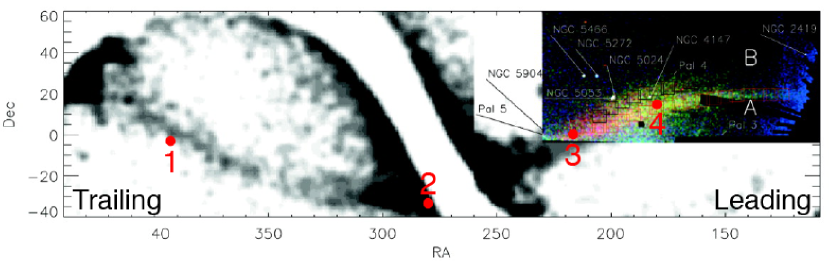
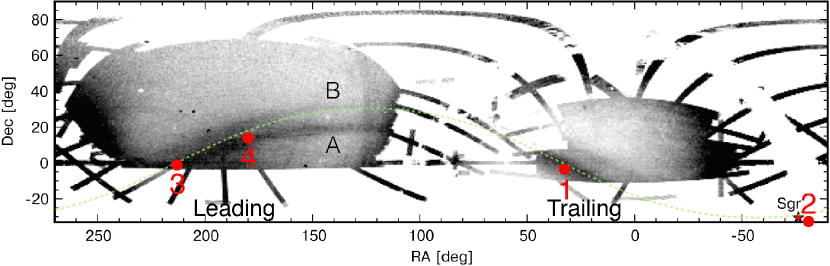
Figure 1.— Two views of the Sagittarius stream in equatorial coordinates, as it circles the celestial sphere. Top panel (Figure 2 of Belokurov et al., 2006): The greyscale reflects the density of M giants selected from 2MASS (Majewski et al., 2003), while the color-map reflects the density of SDSS-selected Stream stars. Bottom panel (Figure 1a of Koposov et al., 2012): The greyscale reflects the density of main-sequence turnoff stars from the SDSS DR8. The green dashed line is the projection of the Sagittarius orbital plane as defined by Majewski et al. (2003). The right ascension ranges of the two panels are shifted relative to each other by $\sim 180^{\circ}$ (in the top panel, the present location of the Sagittarius dwarf spheroidal galaxy is in the middle of the RA range; in the bottom panel it is near the right edge, marked by a red star). The trailing and leading arms of the stream are labeled in each panel. The leading arm bifurcates into branches labeled A and B (following the nomenclature of Belokurov et al., 2006). In both panels, the locations of our HST target fields are indicated with numbered red dots.

2.2. Second-epoch Data

The second-epoch data were obtained by us between 2012 April and October in the context of our science program GO-12564 (PI: R. P. van der Marel). To enable an optimal astrometric analysis, we used ACS/WFC with the same filters used in the first-epoch observations. At the end of each observing sequence for FIELDS 1, 3, and 4, we also included short (total exposure times of $\sim 2,500$ s per field) $V$-band observations in the F606W filter. These enable the construction of CMDs, which are necessary for the identification of Sgr stream stars. We matched the orientation and field centers of the second-epoch observations as closely as possible to those of the first-epoch observations. However, due to unavailability of the same guide stars used for the first-epoch observations, our second-epoch observations for some of the fields required slight differences in the field centers and/or field orientations.

Table 1 lists also the relevant characteristics of the second-epoch observations. The exposure times were chosen to provide a sufficient signal-to-noise ratio for a sufficient number of stream stars and background galaxies in each field to enable accurate PM determinations. The time baselines between the epochs range from 6–9 years.

Table 1HST Target Fields and Observations

	R.A.	Decl.	$\Lambda_{\odot}$	$B_{\odot}$	Epoch 1				Epoch 2 (Prog. ID 12564)
Target	(J2000)	(J2000)	(deg)	(deg)	Prog. ID	Epoch	Exp. Time (s)		Epoch	Exp. Time (s)
FIELD 1	02:09:37.4	$-$04:38:31.6	103.64	3.37	09760	2003.83	10,503		2012.83	7,204
FIELD 2	18:35:45.7	$-$32:59:24.9	356.47	4.75	10775	2006.40	01,700		2012.29	7,390
FIELD 3	14:12:05.7	$-$01:01:52.5	287.05	1.21	10417	2005.37	07,437		2012.37	7,288
FIELD 4	11:59:06.4	$+$13:37:37.9	251.07	4.11	10417	2005.39	05,024		2012.37	6,431

2.3. Astrometric Measurements

We compared the two epochs of $I$-band observations to measure the absolute PMs of individual stars in our target fields. This is accomplished by determining their shifts with respect to distant background galaxies. The method we used for this is similar to the technique that was described and tested extensively in Sohn et al. (2010, 2012). We refer the reader to those studies for more details about the general methodology.

We downloaded the $I$-band _flc.fits images for the first and second epochs from the STScI HST archive. We then determined a position and a flux for each star in each exposure using the img2xym_WFC.09x10 program (Anderson & King, 2006). The positions were corrected for the known ACS/WFC geometric distortions (Anderson & King, 2006) to obtain positions in geometrically rectified frames. Separate distortion solutions were used for the first- and second-epoch data to account for a difference between data taken before and after HST servicing mission SM4 (see Sohn et al., 2010, 2012, for details). For each target field, the first exposure of the first epoch (or the second epoch in the case of field FIELD 2, since that has much deeper data) was selected as the frame of reference. We cross-identified all stars in this exposure with the same stars in the other exposures. The distortion-corrected positions of the cross-identified stars were then used to construct a six-parameter linear transformation between each individual image and the the reference image. We then used these transformations to construct a high-resolution stacked image for each field, with rejection of cosmic rays and image artifacts. For better sampling, the stacked images were super-sampled by a factor of two relative to the native ACS/WFC pixel scale.

We identified stars and background galaxies from the stacked image for each target field. Stars were selected using the quality-of-fit parameter reported by the img2xym_WFC.09x10 program. For background galaxies, we started with catalogs generated by running SExtractor (Bertin & Arnouts, 1996) on the stacked image, and then inspected each candidate source visually to select only bright and compact galaxies.

For each star/galaxy in each of our $I$-band exposures of each target field, we then measured a position using the template-fitting method described in Sohn et al. (2010, 2012). These positions were then corrected for the geometric distortion as before, for use in our subsequent analysis.

The templates we used were constructed from the high-resolution stacked images via a bicubic convolution interpolation method. The templates were directly fitted to the stars and galaxies in exposures of the same epoch for which the stacked images were created. But when fitting templates to exposures in the other epoch, we applied additional 7$\times$7 pixel convolution kernels to account for small PSF differences between the two epochs. For FIELD 2, these kernels were derived using the many bright and isolated stars in the field (members of the globular cluster NGC 6652), similar to what was done in our analyses of M31 and Leo I (Sohn et al., 2012, 2013). However, for FIELDS 1, 3, and 4, there were not enough stars in the field to derive reliable kernels. So for these fields we used an alternative method based on library PSFs, as described in Appendix A.

2.4. Proper Motion Measurements

The next step in the analysis is to transform the geometrically-corrected, template-fitted positions for all sources in all exposures into the reference frame. For this we used a different procedure for FIELD 2 than for the other fields. FIELD 2 is a dense globular cluster field, whereas the other fields are sparse deep fields with very few stars. We describe the procedure for each of these situations in turn.

For FIELD 2, NGC 6652 stars that are distributed throughout the frame were used as reference sources. Since the majority of the stars in this field are NGC 6652 stars, it was easy to select them using their position in CMD and PM diagrams, as discussed in Section 3 below. The distortion-corrected positions of these NGC 6652 stars were used to determine six-parameter linear transformations with respect to the reference frame. These linear transformations were used to transform the measured positions of all stars and background galaxies in all exposures of both epochs into the reference frame. In the reference frame, the mean PM of NGC 6652 is now zero by construction, so that it sets the astrometric zero point.

The individual exposures yield multiple determinations for the position of each star or background galaxy in each epoch. We compute the mean (with outlier rejection) of these determinations to obtain the average position of each source in each epoch. In addition, the rms scatter of the multiple measurements in a given epoch yields the random positional uncertainty in a single measurement, and the error in the mean is then the rms scatter divided by $\sqrt{N}$, where $N$ is the number of measurements in the epoch.

To obtain the absolute proper motion $\mu_{i}$ of each star $i$ in FIELD 2, we first measured its relative motion $\mu^{\prime}_{i}$ with respect to the bulk motion of NGC 6652. This was obtained by taking the difference in reference-frame position between the second and the first epoch, and dividing by the time baseline. Similarly, we measured the apparent relative PM $\mu^{\prime}_{j}$ of each background galaxy $j$ with respect to the bulk motion of NGC 6652. We then took the weighted average of the $\mu^{\prime}_{j}$ over all background galaxies to obtain the bulk motion ${\overline{\mu}^{\prime}_{\rm bg}}$ of all the background galaxies with respect to the bulk motion of NGC 6652.

The absolute PM of a given star is then

$$\mu_{i}=\mu^{\prime}_{i}-{\overline{\mu}^{\prime}_{\rm bg}}.$$ (1)

Random errors were propagated by adding the errors in each step in quadrature, i.e.,

$$\Delta{\mu_{i}}=\sqrt{\Delta{\mu^{\prime}_{i}}^{2}+\Delta{\overline{\mu}^{\prime}_{\rm bg}}^{2}}.$$ (2)

As a byproduct of this process, we also obtain the absolute PM of NGC 6652, $\mu_{\rm NGC6652}=-{\overline{\mu}^{\prime}_{\rm bg}}$, which will be discussed in Appendix B.

For FIELDS 1, 3, and 4, the distortion-corrected positions of background galaxies were directly used to define the astrometric zero point. Again, for each individual exposure, we determined six-parameter linear transformations to match the positions of background galaxies to those in the reference frame. We then used these transformations to transform the measured positions of all sources in all exposures of both epochs into the reference frame.

Since in this approach the frame of reference is defined using distant galaxies in the background, the absolute PM of a given star is simply equal to the difference between the average second- and first-epoch reference frame positions, divided by the time baseline. As before, the PM error for each star is given by equation (2).

The PMs and their associated errors along the detector axes were transformed to the directions west and north using the orientation of each reference image with respect to the sky.

A consistency check on the accuracy of our astrometric reference frame is provided by the fact that one of our fields contains a known distant QSO that is unsaturated in our science exposures. Using the methods described above, we determined the absolute PM of the QSO in FIELD 3 with respect to the reference frame defined by the distant background galaxies. This yields, $(\mu_{W},\mu_{N})=(0.034\pm 0.100,0.068\pm 0.101)\ \>{\rm mas}\,{\rm yr}^{-1}$, which is consistent with zero as expected.

In principle, one could also have used the QSO to set the absolute reference frame in FIELD 3, instead of the background galaxies (as in, e.g., the study of the Magellanic Clouds by Kallivayalil et al., 2013). However, this yields lower accuracy, because the positions of a group of background galaxies can on average be determined more accurately than the position of a single QSO.

The techniques and data we used here to determine PMs are similar to those used in our previous work on M31 and Leo I (Sohn et al., 2012, 2013). The techniques have many built-in features to reduce the potential for systematic errors. Based on extensive tests and comparisons performed in the context of these prior studies (as summarized in Section 2.4 of Sohn et al., 2013), we expect residual systematic PM errors to be $\lesssim 0.03\ \>{\rm mas}\,{\rm yr}^{-1}$. This is lower than the random PM measurement errors that we present below, both for individual stars and for the overall stellar population in the Sgr stream. Possible systematic errors should therefore have a minimal impact on any data-model comparisons.

2.5. Photometric Measurements

Photometric measurements of stars in our target fields are automatically carried out by the img2xym_WFC.09x10 program when measuring library PSF-based positions in the early stage of data analysis. These measurements are in instrumental magnitudes (counts) To calibrate the photometry to the VEGAMAG system, we applied the time-dependent zero points provided by STScI. To determine the appropriate aperture corrections, we made use of the multi-drizzled images of our target fields provided by the HST archive. On these images we measured the brightnesses of several bright and isolated stars using aperture radii of 10 pixels ($0\farcs 5$). The sky backgrounds were measured within 20 to 30 pixels. To correct for the stellar light contributing to the sky background level, we used the encircled energy curves listed in Table 3 of Sirianni et al. (2005). We then further corrected our photometry to an infinite aperture using Table 5 of Sirianni et al. (2005). We then compared the magnitudes to the img2xym_WFC.09x10 program results for the same stars, to determine the appropriate aperture corrections. These were then applied to all stars in our photometric catalogs.

3. Identification of Sagittarius Stream Stars

3.1. Methodology

Our target fields contain stars that belong to the Sgr stream, but also contain MW stars in the foreground or background. Since our goal is to characterize the kinematics of the stream, the identification of Sgr stream stars is crucial. We do this for each field on the basis of two main sources of information: (1) the CMD constructed using the photometry obtained from the measurements in Section 2.5; and (2) the absolute PM $(\mu_{W},\mu_{N})$ vector point diagram obtained from the measurements in Section 2.4. To interpret the information, we make reference to the predictions of stellar population models and dynamical models.

3.1.1 Isochrones

To identify which stars in the CMD (Figures 2a –5a) are consistent with belonging to the Sgr stream, we generally overlay fiducial isochrones developed by the Dartmouth Stellar Evolution Database (DSED, Dotter et al., 2008). For this we use two different stellar populations: an old metal-poor (OMP) population with (age, [Fe/H], [$\alpha$/Fe]) = (13 Gyr, $-1.8$, $+0.2$); and an intermediate metal-rich (IMR) population (5 Gyr, $-0.5$, $0.0$). The age and metallicity combinations were selected based on the HST CMD study of the field around M54 by Siegel et al. (2007), and the [$\alpha$/Fe] value for each metallicity was chosen based on the [Ti/Fe] versus [Fe/H] relation of Sgr stream stars studied by Chou et al. (2010). Our FIELD 1 is close to (but not overlapping with) the SA 93 field of Carlin et al. (2012), and our choice of metallicities is consistent with the two peaks in their metallicity distributions.

For the reddening applied to the isochrones, we took the E($B-V$) value estimated from interpolating the reddening maps of Schlegel, Finkbeiner, & Davis (1998). We added 0.02 of extra reddening as suggested by Siegel et al. (2011). The absorption values $A_{\rm F814W}$ and $A_{\rm F606W}$ were then adopted from Table 6 of Schlafly & Finkbeiner (2011).

For the distances applied to the isochrones, we started from the estimates for each field derived in Paper II. These are based on interpolation of the stream’s known distance variations as function of Sgr longitude, as previously measured from ground-based data by Belokurov et al. (2006, 2014), Koposov et al. (2012) and Slater et al. (2013). To these distances we then applied small corrections at the $\sim 10$% level, to improve the fit to either the observed CMDs or to other observational constraints modeled in Paper II.

The exact choices for the stream’s stellar population properties, reddening, or distance are not critical for the present paper. We are merely trying to determine here which stars in each observed CMD are plausibly associated with the stream. We are not trying to actually fit the CMD, to determine either the stream’s stellar population properties or its distance. Most of our fields are much too sparse to make this practical. Such studies are better carried out with ground-based data that cover larger fields of view.

3.1.2 Sagittarius Stream Dynamical Models

In Figures 2c–5c, we show for comparison as fiducial model for each field the PM predictions of LM10. Their best-fitting $N$-body model for the Sgr stream includes the PM for each model particle. To obtain adequate statistics, we consider for each field those model particles that are within 1.5° in both right ascension and declination from the center of the observed HST field. We use different symbols to indicate whether particles are part of the leading or trailing arm, and whether they are part of the first or second wrap of the stream. We also use different colors as in LM10 to indicate the time at which each particle was stripped. The primary goal of showing the LM10 model predictions is to aid in the identification of features or clumps in the observed PM diagrams. The goal at this stage is not to perform detailed quantitative data-model comparisons. Those are presented in Paper II.

An important goal of the present study is to determine the PMs along the Sgr stream, so that they can be compared to model predictions. For this reason, we are careful not to bias our selection of Sgr stream stars in each field by whether or not they follow the LM10 PM predictions. After all, the LM10 model does have some known limitations and it need not be correct. For example, the model does not address the observed bifurcation of the stream on the leading side (Belokurov et al., 2006), and it does not fit the observed distance of the stream at large angular distances on the trailing side (Belokurov et al., 2014). Nonetheless, the LM10 models does fit many properties of the Sgr stream successfully, and it is helpful for the interpretation of the PM diagrams to have some sense of what might plausibly be expected.

3.1.3 Milky Way Dynamical Models

To identify which stars in the PM vector point diagram (Figures 2b–5b) are consistent with belonging to the Sgr stream, we note that the stream is thin and dynamically cold (Majewski et al., 2004; Monaco et al., 2007). Therefore, Sgr stars clump in PM space, as is evident also in the LM10 model predictions shown in Figures 2c–5c. This is the primary property that sets Sgr stream stars apart from other MW populations.

Foreground stars in the MW disk can generally be separated from Sgr stars both on the basis of their CMD properties and their PM properties. The most numerous stars in the disk are faint red dwarfs. Hence, these provide the main MW disk contamination in our fields. At the apparent magnitudes of interest, these stars are typically redder than Sgr stars. Moreover, for these low-luminosity stars to exceed our observational magnitude limit, they tend to be nearby. Hence, their PM distribution has a large spread of several $\>{\rm mas}\,{\rm yr}^{-1}$ (in fact, disk stars in our fields often have PMs that place them outside the plot ranges in our PM diagrams). This was shown using Besancon MW models (Robin et al., 2003) in Deason et al. (2013, , Figure 3). It is also evident in our observations of FIELD 2 (see Figure 3), which will be discussed in Section 3.3 below. This field lies at Galactic coordinates $(l,b)=(1.9^{\circ},-12.0^{\circ})$, and therefore has a very large MW disk (and bulge) contamination. Since the MW disk population is so much more dispersed in PM space than the Sgr populations of interest, it does not affect any of our subsequent discussion.

Discriminating Sgr stars from MW halo stars is also possible, but not quite as easy. Since halo stars are also part of a pre-dominantly old population, and are found at similar distances as Sgr stars, they cannot be separated purely based on their CMD location. It is therefore important to understand the predicted location of halo stars in PM space. The MW halo does not possess significant rotation. Therefore, to lowest order, the mean transverse velocity of halo stars at any given distance is merely the projection of the solar reflex velocity. This defines a mean PM direction on the plane of the sky. The size of the mean PM for halo stars at a given distance is inversely proportional to the distance.

The mean PM of halo stars differs from the mean PM of Sgr stars. Since our Sun is located close to the Galactic Center, the observed PMs of distant populations reflect primarily the tangential component of the motion in the Galactocentric rest frame. In this frame, Sgr stars have a definite sense of rotation while halo stars do not (for reference, a velocity difference of $200\ \>{\rm km}\,{\rm s}^{-1}$ at $40\ \>{\rm kpc}$ corresponds to $\sim 1\ \>{\rm mas}\,{\rm yr}^{-1}$ PM difference). The typical distance of MW halo stars at the apparent magnitudes of relevance for our HST data is $\sim 25\ \>{\rm kpc}$ (Deason et al., 2013). At this distance, a halo velocity dispersion of $\sim 100\ \>{\rm km}\,{\rm s}^{-1}$ corresponds to a PM dispersion of $\sim 0.8\ \>{\rm mas}\,{\rm yr}^{-1}$; but the actual PM dispersion of halo stars is larger because of the spread in stellar distances. These arguments imply that generally the distributions of Sgr and halo stars will have different means in PM space, but they may be partially overlapping. The Sgr population can be identified because it is the more concentrated of the two. Moreover, because our pointings are located on the Sgr stream, we expect to find more Sgr stars than halo stars in our fields.

To quantitatively predict the PM distribution of MW halo stars in our fields, we used the updated version of the Besancon MW models (Robin et al., 2014). We selected from the Monte-Carlo simulated models only those stars that pass our CMD selection criteria. We then determined for each component of the predicted PMs the median value and the 68-percent confidence interval. These are shown as a red cross in each of Figures 2c, 4c, and 5c (as explained above, the location of each cross corresponds roughly to the reflex motion of the Sun as seen at the median distance of the halo sample). Roughly half of the MW halo stars in our fields that pass our CMD selection criteria are expected within the PM area spanned by these crosses (since, $0.68^{2}=0.46$). This corresponds to an expectation value of $\sim 5$ stars; the actual number varies by field as listed in the figure captions. Due to incompleteness at the faint end (not modeled here), not all of these stars would actually be expected in our samples. Since the predicted numbers of stars are so small, we would expect significant Poisson fluctuations. Moreover, the real MW halo is likely to have more substructure than the smooth Besancon models, which would cause additional fluctuations. And finally, the Besancon models do not reflect all of our latest understanding of the MW halo (e.g., Deason et al., 2014). Therefore, the predictions should be taken as a rough guide only. We ignore the contribution of the MW halo for FIELD 2, located near the Sgr dSph, since Sgr stars in this field vastly outnumber any possible MW halo contamination.

3.2. FIELD 1

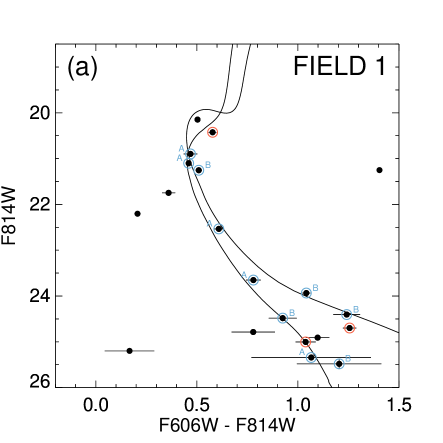
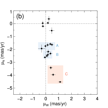
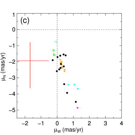
Figure 2.— Selection of stars associated with the Sgr stream in FIELD 1. Panel (a) shows the observed $I$ vs. $V-I$ CMD; panel (b) shows the observed PM diagram; and panel (c) shows for comparison the PM distribution of $N$-body particles in the model of LM10, as well as the predicted location of MW halo stars (red cross). The observed stars in the field are shown as black symbols in all panels, with the associated error bars shown only in panels (a) and (b). Not all stars in panel (a) are shown in panel (b) due to their PMs being outside the range of panel (b). In panel (c) we only show stars identified as Sgr stream stars, and we omit their PM error bars to avoid confusion. The $I$-magnitude errors in panel (a) are smaller than the plot symbols. The black curves in panel (a) are fiducial isochrones for an old metal-poor and an intermediate-age metal-rich population (the latter having the brighter turn-off and redder colors), as described in the text. Colored and labeled boxes in panel (b) highlight stars that likely belong to the Sgr stream, as discussed in the text. The stars in these boxes are circled in their corresponding color and labeled accordingly in panel (a). The particles from the LM10 $N$-body model in panel (c) are color-coded following LM10 such that different colors represent the time at which a given debris particle became unbound from the Sgr dSph: orange for 0 to 1.5 Gyr ago; magenta for 1.5 to 3 Gyr ago; cyan for 3 to 5 Gyr ago; and green for 5 to 7 Gyr ago. Right- and left-facing triangles correspond to stars that belong to the leading and trailing arm of Sgr stream, respectively. Solid/open triangles correspond to the first/second wrap of the stream. The red cross shows the 68 percent confidence intervals in each coordinate for MW halo star PMs drawn from Besancon models, chosen to meet our CMD selection criteria. An expectation value of 3 MW halo stars is predicted within the area spanned by the cross.

Figure 2 shows the CMD (panel a), the PM diagram (panel b) and the LM10 PM predictions (panel c) for FIELD 1. This field is located in the trailing arm of the Sgr stream, $\sim 104^{\circ}$ from the main body of the Sgr dSph (see Figure 1). We measured photometry and PMs of all detected stars in this field, and rejected stars with 1-D PM errors of $>0.3\ \>{\rm mas}\,{\rm yr}^{-1}$. A total of 21 stars were considered for further analysis. Their magnitudes and PMs are shown using black symbols in each panel. The adopted distance for the overlaid isochrones in the CMD is $33.4\ \>{\rm kpc}$; for comparison, the median distance of the LM10 model particles is $30.0\ \>{\rm kpc}$.

Inspection of the CMD shows that most stars fall along one of the two isochrones. Most of these stars are located along a feature in the PM diagram that runs roughly from $(\mu_{W},\mu_{N})\approx(0,-1.5)\ \>{\rm mas}\,{\rm yr}^{-1}$ to $(\mu_{W},\mu_{N})\approx(1,-4.5)\ \>{\rm mas}\,{\rm yr}^{-1}$. A similar PM feature is seen in the LM10 model predictions. So even though the field is sparse, we conclude from the combined CMD and PM data that we have confidently detected the Sgr stream. The stars detected in other parts of the PM diagram and with CMD properties that are inconsistent with the fiducial isochrones are likely foreground or background objects.

Based on the apparent clustering in the PM diagram, we detect four groups of stars. We denote three of the groups as A, B, and C, as indicated in Figure 2b, and discussed below. The fourth group consists of five stars near the PM zero point. Most of these may be unresolved compact background galaxies that are indistinguishable from stars. This interpretation also seems reasonable because these objects do not correspond to any kinematical component predicted by the LM10 model. We note that similar types of objects were detected in our other PM studies, and in those cases we drew the same conclusions. For these reasons, we do not discuss this fourth group of stars further.

None of the groups A, B, or C have the characteristics expected for a MW halo population (red cross in Figure 2c). We therefore identify these groups as Sgr populations. The PMs of the individual stars in these groups are listed in Table 2. It is not obvious that A and B would have to be physically distinct groups, but the PM diagram does suggest the possible presence of two separate clumps. Colored circles and labels in Figure 2a indicate which star belongs to which group. There is no unique one-to-one association between the PM groups and the OMP or IMR isochrones.

Comparison to the LM10 model suggests that stars in group B are associated with the trailing arm, and that they have been recently ($\lesssim 1.5$ Gyr ago) stripped from the main body of the Sgr dSph. Most likely, the same is true for the stars in group A. Alternatively, their PMs are somewhat consistent with those predicted by LM10 for stars in the second wrap of the leading arm. But there are as many stars in group A as group B, and we would normally expect the second wrap to be less populated than the first one. So we do not unambiguously detect second-wrap stars in FIELD 1, but it is possible that they may be present.

The three stars in group C appear to be associated with the leading arm and have been on that part of the stream for at least 3–4 Gyr. In the LM10 model, these leading-arm stars are a factor $\sim 2$ closer than the trailing-arm stars. The positions of the C stars (circled red) in the CMD do not appear inconsistent with this, but there is not enough information to actually determine their distance unambiguously.

It is striking that the accuracy of our data is sufficient not only to detect the Sgr stream, but even to detect different kinematical components of the stream. We can identify individual stars in the same field as belonging to either the trailing or the leading arm, based on their PMs. This amazing result is made possible due to the excellent astrometric capabilities of HST.

Table 2Proper motions and photometry of Sgr stream stars in FIELD 1

	$\mu_{W}$	$\mu_{N}$	F814W	F606W
ID	($\>{\rm mas}\,{\rm yr}^{-1}$)	($\>{\rm mas}\,{\rm yr}^{-1}$)	(VEGAMAG)	(VEGAMAG)
Group A
1	$-$0.02 $\pm$ 0.10	$-$1.74 $\pm$ 0.08	20.90 $\pm$ 0.01	21.37 $\pm$ 0.03
2	string0.35 $\pm$ 0.12	$-$1.58 $\pm$ 0.12	21.10 $\pm$ 0.01	21.56 $\pm$ 0.01
3	string0.48 $\pm$ 0.13	$-$1.64 $\pm$ 0.13	22.53 $\pm$ 0.01	23.14 $\pm$ 0.02
4	string0.15 $\pm$ 0.16	$-$1.66 $\pm$ 0.16	23.65 $\pm$ 0.02	24.43 $\pm$ 0.03
5	$-$0.32 $\pm$ 0.27	$-$1.93 $\pm$ 0.30	25.34 $\pm$ 0.07	26.41 $\pm$ 0.29
Group B
6	$-$0.06 $\pm$ 0.10	$-$2.62 $\pm$ 0.09	21.25 $\pm$ 0.01	21.76 $\pm$ 0.01
7	string0.08 $\pm$ 0.10	$-$2.51 $\pm$ 0.12	23.94 $\pm$ 0.02	24.98 $\pm$ 0.00
8	string0.19 $\pm$ 0.15	$-$2.17 $\pm$ 0.16	24.41 $\pm$ 0.03	25.65 $\pm$ 0.06
9	string0.37 $\pm$ 0.15	$-$2.32 $\pm$ 0.14	24.48 $\pm$ 0.06	25.41 $\pm$ 0.03
10	string0.17 $\pm$ 0.15	$-$2.42 $\pm$ 0.21	25.48 $\pm$ 0.10	26.69 $\pm$ 0.18
Group C
11	string1.12 $\pm$ 0.16	$-$4.52 $\pm$ 0.06	20.43 $\pm$ 0.01	21.00 $\pm$ 0.02
12	string0.58 $\pm$ 0.18	$-$3.96 $\pm$ 0.11	24.70 $\pm$ 0.02	25.96 $\pm$ 0.02
13	string0.39 $\pm$ 0.15	$-$3.42 $\pm$ 0.13	25.00 $\pm$ 0.05	26.04 $\pm$ 0.02

3.3. FIELD 2

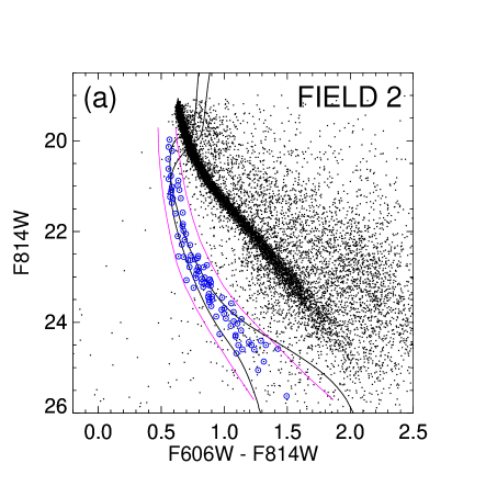
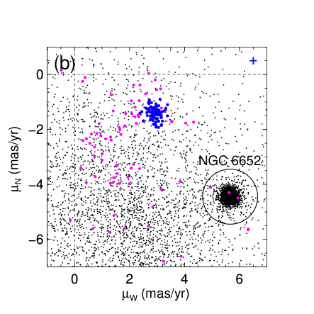
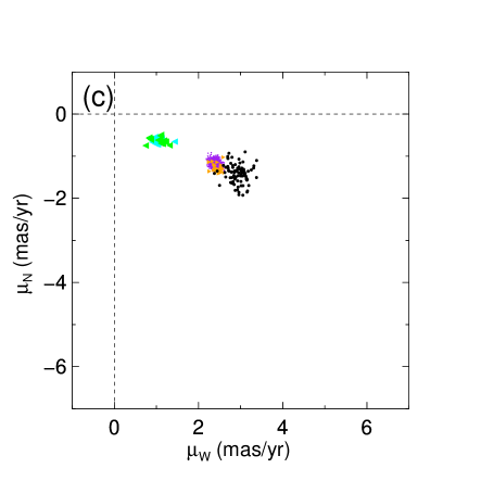
Figure 3.— Selection of stars associated with the Sgr stream in FIELD 2. The panels and symbols are generally similar to those in Figure 2, but with some exceptions as noted below. FIELD 2 is centered on the globular cluster NGC 6652. The globular cluster stars are easily recognized by their MS in the CMD, and their clustering in PM space, as indicated in panel (b). The Sgr stream stars in the background outline a secondary MS in the CMD, blueward of the NGC 6652 MS. We define candidate Sgr stream stars as lying between the magenta lines. In panel (b), blue-colored stars (also circled blue in panel (a), and shown in black in panel (c)) are those that survive a 3-$\sigma$ clipping algorithm in PM space. Magenta-colored stars are those that are not consistent at the 3-$\sigma$ level with the weighted mean PM of the blue-colored stars. Individual PM error bars are not shown to avoid confusion. The blue cross in the top right of panel (b) indicates the median PM error bars for the blue points. The black points that are widely scattered over the PM diagram are mostly Milky Way disk and bulge field stars. The groups of green and cyan symbols in panel (c) consists entirely of trailing particles, while the group of orange symbols consists entirely of leading particles. Purple dots that largely overlap with the orange triangles are LM10 model particles that are bound to the Sgr dSph. There are 465 purple dots and 28 orange triangles near $(\mu_{W},\mu_{N})=(2.4,-1.2)\ \>{\rm mas}\,{\rm yr}^{-1}$.

Figure 3 shows the CMD, the PM diagram, and the LM10 PM predictions for FIELD 2. This field is located in the leading arm of the Sgr stream, but it is close to ($\sim 4^{\circ}$ away from) the main body of the Sgr dSph (see Figure 1). The field is centered on the globular cluster NGC 6652, and its main sequence (MS) dominates the CMD. But as pointed out by Siegel et al. (2011), the MS of the Sgr stars in the background is readily visible as a faint secondary sequence roughly parallel to and below the MS of NGC 6652. The adopted distance for the overlaid isochrones in the CMD is $30.5\ \>{\rm kpc}$; for comparison, the median distance of the LM10 model particles is $28.4\ \>{\rm kpc}$. The distance of NGC 6652 is $10.5\ \>{\rm kpc}$.

Since the angular distance to the Sgr dSph core is much smaller than for the other HST fields (see Figure 1), it has a much higher density of Sgr stars. This makes the selection of these stars in the CMD straightforward. We define candidate Sgr stars as those stars lying between the magenta lines in Figure 3a. This yields 90 candidate Sgr stars, out of $>12,000$ total stars identified in the field.

The PM distribution of the stars in FIELD 2, shown in Figure 3b, has the two conspicuous clumps that are readily identified. One clump at $(\mu_{W},\mu_{N})\approx(5.5,-4.5)\ \>{\rm mas}\,{\rm yr}^{-1}$ is due to stars in NGC 6652. The other clump at $(\mu_{W},\mu_{N})\approx(2.9,-1.4)\ \>{\rm mas}\,{\rm yr}^{-1}$ is due to Sgr stream stars. The remaining stars that are widely scattered over the PM diagram are mostly MW disk and bulge field stars. All these results are qualitatively similar to those reported by Massari et al. (2013) for NGC 6681, another MW globular cluster towards the Galactic Bulge that has Sgr stars in the background.

To obtain a final selection of Sgr stream stars, we first determined the mean PM of all the candidate stars identified from the CMD. We then applied an iterative 3-$\sigma$ rejection to reject those stars (shown in magenta color) with PMs inconsistent with this mean. We identify the remaining 90 stars (shown in blue) as bona-fide Sgr stream stars. The PMs of these individual stars are listed in Table 3.

The observed PM clump in Figure 3c shows reasonable agreement with the LM10 $N$-body model particles on the leading arm that are either currently bound to the Sgr dSph (purple dots) or recently became unbound (orange triangles). This indicates that the majority of stars in the observed clump are bound to the Sgr dSph and belong to the leading arm (as expected, since the field is on the leading arm of the Sgr stream). Interestingly, while the PM direction of the observed stars is the same as in the model, the size of the observed PMs appears to be somewhat larger by $\sim 0.5\ \>{\rm mas}\,{\rm yr}^{-1}$. We discuss this discrepancy in Section 4.3.

In this field, the LM10 model also predicts, at a different location in PM space, the presence of trailing-arm particles (green and cyan triangles) that are almost $360^{\circ}$ wrapped from the main body. Although this clump of particles appear to be conspicuous in Figure 3c, it consist of only 41 model particles, i.e., $\sim 8$% of total number of leading-arm model particles. This means the model predicts about 7 trailing-arm stars in this field. We do not find stars with PMs consistent with these particles in our data. Given that the trailing-arm model particles lie at further distance than the leading-arm particles (at an average distance of $\sim 47\ \>{\rm kpc}$), we expanded our search in the CMD to look for the trailing-arm stars but did not find any. This may indicate that the model overpredicts the density of particles at large angular distances from the main body of the Sgr dSph, or that it incorrectly predicts their location. Alternatively, it may simply be due to small number statistics.

Table 3Proper motions and photometry of Sgr stream stars in FIELD 2

	$\mu_{W}$	$\mu_{N}$	F814W	F606W
ID	($\>{\rm mas}\,{\rm yr}^{-1}$)	($\>{\rm mas}\,{\rm yr}^{-1}$)	(VEGAMAG)	(VEGAMAG)
1	3.04 $\pm$ 0.10	$-$1.39 $\pm$ 0.22	19.97 $\pm$ 0.00	20.54 $\pm$ 0.01
2	2.90 $\pm$ 0.11	$-$1.38 $\pm$ 0.13	20.13 $\pm$ 0.01	20.69 $\pm$ 0.01
3	3.02 $\pm$ 0.09	$-$1.36 $\pm$ 0.11	20.22 $\pm$ 0.01	20.81 $\pm$ 0.00
4	3.00 $\pm$ 0.09	$-$1.37 $\pm$ 0.13	20.40 $\pm$ 0.01	20.96 $\pm$ 0.10
5	3.09 $\pm$ 0.09	$-$1.42 $\pm$ 0.14	20.62 $\pm$ 0.01	21.18 $\pm$ 0.01
6	2.86 $\pm$ 0.08	$-$1.37 $\pm$ 0.11	20.77 $\pm$ 0.01	21.35 $\pm$ 0.01
7	3.13 $\pm$ 0.16	$-$1.58 $\pm$ 0.14	20.84 $\pm$ 0.00	21.40 $\pm$ 0.01
8	3.05 $\pm$ 0.11	$-$1.32 $\pm$ 0.11	20.88 $\pm$ 0.01	21.52 $\pm$ 0.00
9	2.94 $\pm$ 0.10	$-$1.09 $\pm$ 0.14	20.98 $\pm$ 0.05	21.61 $\pm$ 0.01
10	2.68 $\pm$ 0.21	$-$1.26 $\pm$ 0.14	21.02 $\pm$ 0.01	21.60 $\pm$ 0.00
11	2.86 $\pm$ 0.09	$-$1.21 $\pm$ 0.18	21.08 $\pm$ 0.01	21.73 $\pm$ 0.00
12	2.80 $\pm$ 0.11	$-$1.62 $\pm$ 0.14	21.09 $\pm$ 0.01	21.67 $\pm$ 0.01
13	2.99 $\pm$ 0.11	$-$1.45 $\pm$ 0.16	21.13 $\pm$ 0.01	21.71 $\pm$ 0.02
14	2.75 $\pm$ 0.15	$-$1.18 $\pm$ 0.19	21.24 $\pm$ 0.01	21.81 $\pm$ 0.01
15	3.24 $\pm$ 0.10	$-$1.34 $\pm$ 0.11	21.27 $\pm$ 0.01	21.92 $\pm$ 0.01
16	2.76 $\pm$ 0.11	$-$1.39 $\pm$ 0.15	21.27 $\pm$ 0.01	21.86 $\pm$ 0.01
17	3.01 $\pm$ 0.09	$-$1.38 $\pm$ 0.14	21.37 $\pm$ 0.01	21.95 $\pm$ 0.06
18	2.78 $\pm$ 0.16	$-$1.52 $\pm$ 0.12	21.58 $\pm$ 0.01	22.26 $\pm$ 0.02
19	2.70 $\pm$ 0.12	$-$1.36 $\pm$ 0.12	21.60 $\pm$ 0.01	22.22 $\pm$ 0.01
20	3.03 $\pm$ 0.13	$-$1.40 $\pm$ 0.14	21.83 $\pm$ 0.02	22.51 $\pm$ 0.01
21	2.94 $\pm$ 0.08	$-$1.27 $\pm$ 0.22	21.88 $\pm$ 0.01	22.55 $\pm$ 0.01
22	2.90 $\pm$ 0.22	$-$1.35 $\pm$ 0.17	21.98 $\pm$ 0.01	22.66 $\pm$ 0.00
23	2.92 $\pm$ 0.15	$-$1.75 $\pm$ 0.17	22.05 $\pm$ 0.01	22.75 $\pm$ 0.01
24	2.68 $\pm$ 0.11	$-$1.06 $\pm$ 0.15	22.10 $\pm$ 0.01	22.73 $\pm$ 0.00
25	3.08 $\pm$ 0.11	$-$1.44 $\pm$ 0.12	22.18 $\pm$ 0.01	22.87 $\pm$ 0.00
26	2.85 $\pm$ 0.14	$-$1.52 $\pm$ 0.18	22.29 $\pm$ 0.01	22.95 $\pm$ 0.01
27	2.94 $\pm$ 0.13	$-$1.42 $\pm$ 0.19	22.30 $\pm$ 0.01	23.03 $\pm$ 0.02
28	2.32 $\pm$ 0.15	$-$1.56 $\pm$ 0.19	22.53 $\pm$ 0.02	23.26 $\pm$ 0.00
29	2.63 $\pm$ 0.11	$-$1.51 $\pm$ 0.17	22.54 $\pm$ 0.01	23.33 $\pm$ 0.01
30	3.16 $\pm$ 0.19	$-$1.37 $\pm$ 0.17	22.55 $\pm$ 0.02	23.19 $\pm$ 0.14
31	2.61 $\pm$ 0.10	$-$1.40 $\pm$ 0.13	22.56 $\pm$ 0.02	23.24 $\pm$ 0.02
32	3.01 $\pm$ 0.10	$-$1.30 $\pm$ 0.13	22.59 $\pm$ 0.03	23.37 $\pm$ 0.01
33	2.83 $\pm$ 0.15	$-$1.40 $\pm$ 0.14	22.61 $\pm$ 0.02	23.38 $\pm$ 0.02
34	2.69 $\pm$ 0.14	$-$1.30 $\pm$ 0.17	22.63 $\pm$ 0.02	23.34 $\pm$ 0.02
35	3.04 $\pm$ 0.21	$-$1.48 $\pm$ 0.14	22.63 $\pm$ 0.01	23.36 $\pm$ 0.02
36	3.13 $\pm$ 0.12	$-$1.58 $\pm$ 0.21	22.74 $\pm$ 0.00	23.60 $\pm$ 0.03
37	2.91 $\pm$ 0.11	$-$1.48 $\pm$ 0.16	22.78 $\pm$ 0.02	23.51 $\pm$ 0.03
38	3.11 $\pm$ 0.10	$-$1.49 $\pm$ 0.21	22.79 $\pm$ 0.03	23.58 $\pm$ 0.03
39	2.96 $\pm$ 0.10	$-$1.18 $\pm$ 0.15	22.79 $\pm$ 0.02	23.62 $\pm$ 0.05
40	3.07 $\pm$ 0.16	$-$1.42 $\pm$ 0.15	22.85 $\pm$ 0.03	23.64 $\pm$ 0.02
41	2.71 $\pm$ 0.15	$-$1.37 $\pm$ 0.14	22.88 $\pm$ 0.02	23.68 $\pm$ 0.01
42	3.00 $\pm$ 0.16	$-$1.48 $\pm$ 0.21	22.94 $\pm$ 0.01	23.72 $\pm$ 0.02
43	3.15 $\pm$ 0.19	$-$1.84 $\pm$ 0.24	23.02 $\pm$ 0.03	23.86 $\pm$ 0.27
44	2.99 $\pm$ 0.20	$-$1.72 $\pm$ 0.26	23.02 $\pm$ 0.02	23.80 $\pm$ 0.03
45	2.43 $\pm$ 0.08	$-$1.37 $\pm$ 0.11	23.04 $\pm$ 0.04	23.86 $\pm$ 0.00
46	2.36 $\pm$ 0.15	$-$1.42 $\pm$ 0.17	23.06 $\pm$ 0.06	23.94 $\pm$ 0.29
47	2.83 $\pm$ 0.17	$-$1.69 $\pm$ 0.23	23.07 $\pm$ 0.02	23.95 $\pm$ 0.03
48	2.77 $\pm$ 0.13	$-$1.39 $\pm$ 0.16	23.07 $\pm$ 0.01	23.77 $\pm$ 0.15
49	2.94 $\pm$ 0.11	$-$1.87 $\pm$ 0.16	23.12 $\pm$ 0.02	23.94 $\pm$ 0.01
50	3.12 $\pm$ 0.11	$-$1.56 $\pm$ 0.14	23.12 $\pm$ 0.04	24.01 $\pm$ 0.01
51	2.82 $\pm$ 0.18	$-$1.23 $\pm$ 0.21	23.15 $\pm$ 0.03	23.99 $\pm$ 0.00
52	2.80 $\pm$ 0.13	$-$1.28 $\pm$ 0.22	23.18 $\pm$ 0.02	24.05 $\pm$ 0.05
53	2.80 $\pm$ 0.12	$-$1.24 $\pm$ 0.13	23.20 $\pm$ 0.04	24.09 $\pm$ 0.01
54	2.91 $\pm$ 0.19	$-$1.30 $\pm$ 0.22	23.22 $\pm$ 0.02	24.05 $\pm$ 0.03
55	2.82 $\pm$ 0.24	$-$1.47 $\pm$ 0.17	23.24 $\pm$ 0.02	24.00 $\pm$ 0.14
56	2.68 $\pm$ 0.31	$-$1.07 $\pm$ 0.20	23.38 $\pm$ 0.03	24.25 $\pm$ 0.04
57	2.78 $\pm$ 0.15	$-$1.04 $\pm$ 0.24	23.43 $\pm$ 0.02	24.33 $\pm$ 0.05
58	2.63 $\pm$ 0.22	$-$1.28 $\pm$ 0.22	23.44 $\pm$ 0.04	24.31 $\pm$ 0.03
59	3.14 $\pm$ 0.27	$-$1.87 $\pm$ 0.21	23.46 $\pm$ 0.08	24.44 $\pm$ 0.05
60	2.57 $\pm$ 0.15	$-$1.24 $\pm$ 0.22	23.50 $\pm$ 0.02	24.40 $\pm$ 0.02
61	2.18 $\pm$ 0.16	$-$1.20 $\pm$ 0.17	23.50 $\pm$ 0.02	24.38 $\pm$ 0.03
62	2.86 $\pm$ 0.14	$-$1.53 $\pm$ 0.11	23.56 $\pm$ 0.03	24.44 $\pm$ 0.12
63	2.83 $\pm$ 0.14	$-$1.37 $\pm$ 0.17	23.58 $\pm$ 0.02	24.64 $\pm$ 0.03
64	3.14 $\pm$ 0.14	$-$1.23 $\pm$ 0.18	23.64 $\pm$ 0.03	24.54 $\pm$ 0.01
65	2.85 $\pm$ 0.23	$-$1.56 $\pm$ 0.23	23.69 $\pm$ 0.03	24.69 $\pm$ 0.03
66	2.80 $\pm$ 0.16	$-$1.63 $\pm$ 0.17	23.73 $\pm$ 0.04	24.71 $\pm$ 0.02
67	2.74 $\pm$ 0.20	$-$1.53 $\pm$ 0.20	23.78 $\pm$ 0.05	24.85 $\pm$ 0.07
68	3.09 $\pm$ 0.26	$-$0.91 $\pm$ 0.35	23.81 $\pm$ 0.06	24.81 $\pm$ 0.02
69	2.48 $\pm$ 0.21	$-$1.71 $\pm$ 0.19	23.87 $\pm$ 0.03	24.81 $\pm$ 0.03
70	3.12 $\pm$ 0.15	$-$1.53 $\pm$ 0.48	23.91 $\pm$ 0.04	24.93 $\pm$ 0.05

Table 3Continued from previous page.

	$\mu_{W}$	$\mu_{N}$	F814W	F606W
ID	($\>{\rm mas}\,{\rm yr}^{-1}$)	($\>{\rm mas}\,{\rm yr}^{-1}$)	(VEGAMAG)	(VEGAMAG)
71	3.04 $\pm$ 0.18	$-$1.15 $\pm$ 0.21	23.93 $\pm$ 0.07	25.06 $\pm$ 0.03
72	2.77 $\pm$ 0.33	$-$1.65 $\pm$ 0.22	23.98 $\pm$ 0.03	25.06 $\pm$ 0.05
73	2.99 $\pm$ 0.26	$-$1.62 $\pm$ 0.30	24.03 $\pm$ 0.06	25.13 $\pm$ 0.02
74	3.29 $\pm$ 0.18	$-$1.30 $\pm$ 0.18	24.08 $\pm$ 0.04	25.13 $\pm$ 0.07
75	3.14 $\pm$ 0.29	$-$1.57 $\pm$ 0.21	24.18 $\pm$ 0.03	25.31 $\pm$ 0.01
76	2.96 $\pm$ 0.20	$-$1.33 $\pm$ 0.44	24.26 $\pm$ 0.06	25.23 $\pm$ 0.06
77	2.80 $\pm$ 0.25	$-$1.66 $\pm$ 0.42	24.28 $\pm$ 0.04	25.37 $\pm$ 0.01
78	2.91 $\pm$ 0.35	$-$1.60 $\pm$ 0.36	24.32 $\pm$ 0.04	25.41 $\pm$ 0.06
79	2.85 $\pm$ 0.24	$-$1.83 $\pm$ 0.27	24.41 $\pm$ 0.06	25.70 $\pm$ 0.10
80	2.74 $\pm$ 0.35	$-$1.64 $\pm$ 0.40	24.44 $\pm$ 0.05	25.63 $\pm$ 0.02
81	2.70 $\pm$ 0.22	$-$0.94 $\pm$ 0.20	24.50 $\pm$ 0.04	25.72 $\pm$ 0.05
82	3.06 $\pm$ 0.28	$-$1.37 $\pm$ 0.49	24.50 $\pm$ 0.07	25.83 $\pm$ 0.16
83	3.30 $\pm$ 0.45	$-$1.24 $\pm$ 0.34	24.50 $\pm$ 0.07	25.62 $\pm$ 0.08
84	3.36 $\pm$ 0.42	$-$1.12 $\pm$ 0.49	24.58 $\pm$ 0.04	26.01 $\pm$ 0.03
85	2.68 $\pm$ 0.39	$-$1.02 $\pm$ 0.31	24.60 $\pm$ 0.04	25.74 $\pm$ 0.04
86	3.18 $\pm$ 0.40	$-$1.71 $\pm$ 0.65	24.60 $\pm$ 0.07	25.84 $\pm$ 0.05
87	3.51 $\pm$ 0.44	$-$1.74 $\pm$ 0.30	24.69 $\pm$ 0.06	25.78 $\pm$ 0.02
88	3.04 $\pm$ 0.56	$-$1.94 $\pm$ 0.61	24.86 $\pm$ 0.05	26.18 $\pm$ 0.22
89	2.18 $\pm$ 0.25	$-$1.56 $\pm$ 0.38	25.06 $\pm$ 0.08	26.32 $\pm$ 0.13
90	2.29 $\pm$ 0.39	$-$1.49 $\pm$ 0.33	25.63 $\pm$ 0.11	27.12 $\pm$ 0.22

3.4. FIELD 3

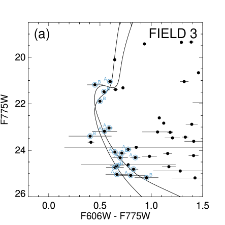
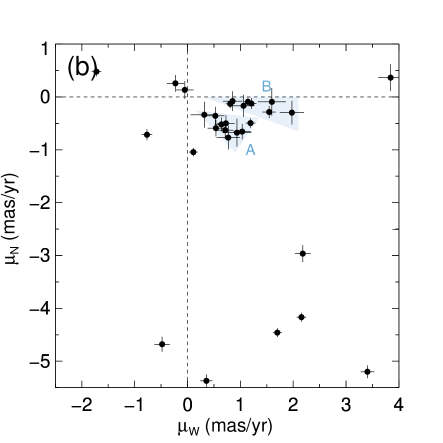
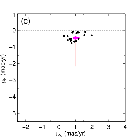
Figure 4.— Selection of stars associated with the Sgr stream in FIELD 3. The panels and symbols are similar to those in Figure 2. The group of magenta symbols in panel (c) consists entirely of leading particles. An expectation value of 3 MW halo stars is predicted within the area spanned by the red cross.

Table 4Proper motions and photometry of Sgr stream stars in FIELD 3

	$\mu_{W}$	$\mu_{N}$	F775W	F606W
ID	($\>{\rm mas}\,{\rm yr}^{-1}$)	($\>{\rm mas}\,{\rm yr}^{-1}$)	(VEGAMAG)	(VEGAMAG)
Group A
1	1.03 $\pm$ 0.16	$-$0.66 $\pm$ 0.15	21.04 $\pm$ 0.01	21.64 $\pm$ 0.01
2	0.71 $\pm$ 0.15	$-$0.63 $\pm$ 0.16	23.04 $\pm$ 0.02	23.63 $\pm$ 0.03
3	1.19 $\pm$ 0.09	$-$0.49 $\pm$ 0.09	23.18 $\pm$ 0.02	23.72 $\pm$ 0.12
4	0.64 $\pm$ 0.12	$-$0.52 $\pm$ 0.13	23.96 $\pm$ 0.02	24.73 $\pm$ 0.02
5	0.53 $\pm$ 0.17	$-$0.36 $\pm$ 0.17	24.07 $\pm$ 0.04	24.72 $\pm$ 0.03
6	0.73 $\pm$ 0.16	$-$0.50 $\pm$ 0.15	24.31 $\pm$ 0.04	25.15 $\pm$ 0.03
7	0.54 $\pm$ 0.16	$-$0.59 $\pm$ 0.16	24.32 $\pm$ 0.06	25.02 $\pm$ 0.04
8	0.32 $\pm$ 0.26	$-$0.34 $\pm$ 0.24	24.81 $\pm$ 0.04	25.64 $\pm$ 0.01
9	0.94 $\pm$ 0.27	$-$0.68 $\pm$ 0.26	25.03 $\pm$ 0.07	25.70 $\pm$ 0.08
10	0.77 $\pm$ 0.22	$-$0.77 $\pm$ 0.22	25.07 $\pm$ 0.05	25.87 $\pm$ 0.13
Group B
11	1.14 $\pm$ 0.07	$-$0.09 $\pm$ 0.07	21.18 $\pm$ 0.01	21.63 $\pm$ 0.08
12	1.21 $\pm$ 0.10	$-$0.12 $\pm$ 0.10	21.48 $\pm$ 0.01	22.02 $\pm$ 0.02
13	1.54 $\pm$ 0.13	$-$0.28 $\pm$ 0.11	21.89 $\pm$ 0.01	22.39 $\pm$ 0.01
14	0.81 $\pm$ 0.08	$-$0.13 $\pm$ 0.08	23.39 $\pm$ 0.02	23.79 $\pm$ 0.21
15	1.06 $\pm$ 0.21	$-$0.17 $\pm$ 0.21	24.12 $\pm$ 0.03	24.83 $\pm$ 0.03
16	1.60 $\pm$ 0.26	$-$0.09 $\pm$ 0.26	24.67 $\pm$ 0.06	25.34 $\pm$ 0.03
17	1.98 $\pm$ 0.23	$-$0.30 $\pm$ 0.22	24.73 $\pm$ 0.05	25.37 $\pm$ 0.07
18	0.85 $\pm$ 0.18	$-$0.08 $\pm$ 0.19	25.18 $\pm$ 0.08	26.13 $\pm$ 0.08

Figure 4 shows the CMD, the PM diagram, and the LM10 PM predictions for FIELD 3. This field is located in the leading arm of the Sgr stream, $\sim 73^{\circ}$ from the main body of the Sgr dSph (see Figure 1). So it is a sparse field, like FIELD 1. However, it has a somewhat higher density of foreground stars, as expected based on its Galactic coordinates, and in particular its Galactic longitude. Among all of the stars detected in this field, a total of 53 stars were considered for further analysis after rejecting stars with 1-D PM errors of $>0.3\ \>{\rm mas}\,{\rm yr}^{-1}$. The adopted distance for the overlaid isochrones in the CMD is $57.8\ \>{\rm kpc}$; for comparison, the median distance of the LM10 model particles is $54.5\ \>{\rm kpc}$. The Sgr stream stars in FIELD 3 have the largest distances among those in all of our HST fields, because this field is located near the apocenter of the leading arm.

We find that many stars in the CMD fall along one of our two fiducial isochrones, and that a majority of these stars are located in the PM diagram in a concentration that stretches roughly from $(\mu_{W},\mu_{N})\approx(0.2,-1.0)\ \>{\rm mas}\,{\rm yr}^{-1}$ to $(\mu_{W},\mu_{N})\approx(2.0,0.0)\ \>{\rm mas}\,{\rm yr}^{-1}$. The LM10 model predictions show a cold clump in more or less the same part of PM space. These model particles are associated with the leading-arm component, and were released from the main Sgr body at 1.5–3 Gyr ago. The LM10 model does not predict trailing-arm or secondary-wrap particles in FIELD 3 (because these particles fall at different Sgr latitude $B_{\odot}$), and indeed, no obvious additional cold clumps are detected in PM space. The stars detected in other parts of the PM diagram are not clumped, and have CMD properties that are inconsistent with the fiducial isochrones (mostly stars with redder colors). So these are likely foreground or background objects.

We identify 18 stars that cluster in PM space, and divide them into two groups denoted A and B, as indicated in Figure 4b. We list the PMs of individual stars in these groups in Table 4. It is not obvious that A and B would have to be physically distinct groups, but the PM diagram does suggest the possible presence of two separate clumps. Colored circles and labels in Figure 4a indicate which star belongs to which group. We find no unique one-to-one association between the PM groups and the OMP or IMR isochrones.

Group B is well separated in PM space from the predicted location of MW halo stars. So we conclude from the combined CMD and PM data that we have confidently detected the leading arm of the Sgr stream. Most likely, group A is also part of the leading arm of the Sgr stream, but this is somewhat less certain. The mean PM of group A is close to the mean PM predicted for MW halo stars in this field. Also, the number of stars in group A is comparable to the predicted number of MW halo stars that pass our CMD cuts (12 stars total, 6 stars in the area spanned by the red cross in Figure 4c). However, group A is significantly colder in PM space than what is predicted for any smooth MW halo population. So either group A is not a MW halo population, or the actual properties of the MW halo must differ significantly from what is assumed in the Besancon models.

3.5. FIELD 4

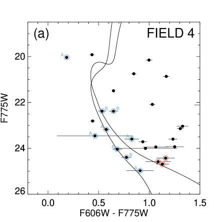
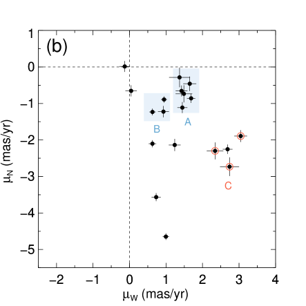
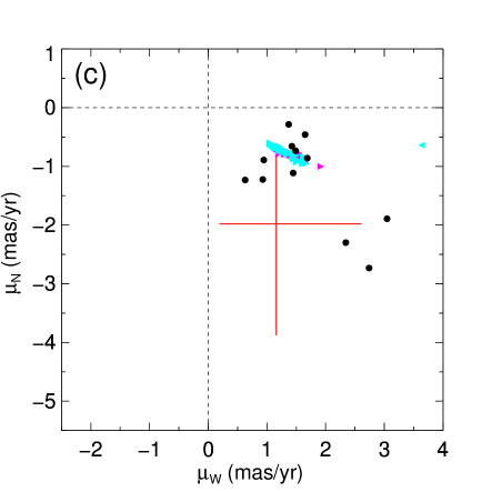
Figure 5.— Selection of stars associated with the Sgr stream in FIELD 4. The panels and symbols are similar to those in Figure 2. The group of cyan and magenta symbols in panel (c) consists entirely of leading particles, except for one trailing particle located far off to the right. An expectation value of 4 MW halo stars is predicted within the area spanned by the red cross.

Table 5Proper motions and photometry of Sgr stream stars in FIELD 4

	$\mu_{W}$	$\mu_{N}$	F775W	F606W
ID	($\>{\rm mas}\,{\rm yr}^{-1}$)	($\>{\rm mas}\,{\rm yr}^{-1}$)	(VEGAMAG)	(VEGAMAG)
Group A
1	1.65 $\pm$ 0.18	$-$0.46 $\pm$ 0.20	20.04 $\pm$ 0.01	20.22 $\pm$ 0.00
2	1.69 $\pm$ 0.11	$-$0.86 $\pm$ 0.12	23.18 $\pm$ 0.03	23.75 $\pm$ 0.02
3	1.45 $\pm$ 0.14	$-$1.11 $\pm$ 0.15	23.45 $\pm$ 0.04	23.92 $\pm$ 0.37
4	1.43 $\pm$ 0.16	$-$0.66 $\pm$ 0.15	23.60 $\pm$ 0.03	24.42 $\pm$ 0.07
5	1.37 $\pm$ 0.29	$-$0.28 $\pm$ 0.27	24.04 $\pm$ 0.05	24.72 $\pm$ 0.01
6	1.49 $\pm$ 0.23	$-$0.73 $\pm$ 0.23	24.97 $\pm$ 0.06	25.88 $\pm$ 0.12
Group B
7	0.95 $\pm$ 0.08	$-$0.89 $\pm$ 0.09	22.38 $\pm$ 0.01	22.91 $\pm$ 0.04
8	0.63 $\pm$ 0.09	$-$1.23 $\pm$ 0.09	22.38 $\pm$ 0.01	23.03 $\pm$ 0.04
9	0.93 $\pm$ 0.15	$-$1.22 $\pm$ 0.16	24.39 $\pm$ 0.04	25.17 $\pm$ 0.03
Group C
10	3.05 $\pm$ 0.17	$-$1.89 $\pm$ 0.16	24.43 $\pm$ 0.04	25.59 $\pm$ 0.08
11	2.34 $\pm$ 0.23	$-$2.30 $\pm$ 0.23	24.58 $\pm$ 0.06	25.67 $\pm$ 0.11
12	2.74 $\pm$ 0.26	$-$2.73 $\pm$ 0.26	24.69 $\pm$ 0.05	25.82 $\pm$ 0.04

Figure 5 shows the CMD, the PM diagram, and the LM10 PM predictions for FIELD 4. This field is located further out in the leading arm of the Sgr stream, $\sim 109^{\circ}$ from the main body of the Sgr dSph (see Figure 1). So it is a sparse field, like FIELD 1 and FIELD 3. Its density of foreground stars is intermediate between those fields, as expected based on its Galactic coordinates, and in particular its Galactic longitude. Among all of the stars detected in this field, a total of 30 stars were considered for further analysis after rejecting stars with 1-D PM errors of $>0.3\ \>{\rm mas}\,{\rm yr}^{-1}$. The adopted distance for the overlaid isochrones in the CMD is $37.8\ \>{\rm kpc}$; for comparison, the median distance of the LM10 model particles is $38.3\ \>{\rm kpc}$.

Inspection of the CMD shows that many stars fall along one of our two fiducial isochrones. Most of the stars consistent with our fiducial isochrones are located in the PM diagram in a concentration around $(\mu_{W},\mu_{N})\approx(1.3,-0.8)\ \>{\rm mas}\,{\rm yr}^{-1}$. The LM10 model particles cluster in more or less the same part of PM space. These model particles are associated with the leading-arm component, and most of them were released from the main Sgr body at 3–5 Gyr ago. This is 1–2 Gyr earlier than the stars in FIELD 3, which is why these stars are now found at a larger angular distance from the Sgr dSph.

We focus on 8 stars observed near the leading arm PM predicted by LM10. Based on the apparent clustering in the PM diagram, we divide these stars into two groups. We denote these groups as A and B, as indicated in Figure 5b. The PMs of the individual stars in these groups are listed in Table 5. As are the cases of FIELDS 1 and 3, it is not obvious that A and B would have to be physically distinct groups, but the PM diagram does suggest the possible presence of two separate clumps. Colored circles and labels in Figure 5a indicate which star belongs to which group. There is no unique one-to-one association between the PM groups and the OMP or IMR isochrones.

Most of the stars detected in other parts of the PM diagram are not clumped, and have CMD properties that are inconsistent with the fiducial isochrones (mostly stars with redder colors). So these are likely foreground or background objects. However, there is some evidence for an additional clump of stars in PM space, which we have labeled “C” in Figure 5b. These stars could represent a coherent cold component, although this cannot be established with statistical significance given the low number of stars.

Group A is well separated in PM space from the predicted location of MW halo stars. So we conclude from the combined CMD and PM data that we have confidently detected the leading arm of the Sgr stream. Whether group B is also part of the Sgr stream is not clear. The mean PM of group B is close to the mean PM predicted for MW halo stars in this field. Also, the number of stars in group B is comparable to the predicted number of MW halo stars that pass our CMD cuts (4 stars in the area spanned by the red cross in Figure 5c). The low number of stars in group B, and the presence of additional stars in the PM diagram which may or may not be associated, makes it difficult to determine whether the PM dispersion of this group is or is not consistent with that predicted for a MW halo population.

Group C could indicate the presence of an unrelated stream in the MW halo, given that the PM of this clump is not consistent with any component seen in the LM10 model. Trailing stream particles at this Sgr longitude $\Lambda_{\odot}$ in the LM10 model are mostly located at different latitude $B_{\odot}$ than FIELD 4 (although one such particle is seen in Figure 5c) and have PMs that cluster near $(\mu_{W},\mu_{N})\approx(4.0,-0.5)$. The median distance of these trailing-arm stars is $21.4\ \>{\rm kpc}$, which is closer than the distance of the leading-arm particles. The CMD properties of the C clump stars (circled red in Figure 5a) are not inconsistent with this. So we cannot rule out that the C clump does in fact represent the trailing arm of the Sgr stream. If so, then the LM10 model does not correctly represent the dynamics of these particles. There is in fact some independent evidence that this may be the case. Specifically, Belokurov et al. (2014) showed that in the trailing arm of the stream, at angular distances $\gtrsim 150^{\circ}$ from the Sgr dSph, the LM10 model may not correctly reproduce the observed stream distances. In view of this, we cannot at present uniquely identify the nature of the C clump stars in FIELD 4.

Table 6Proper Motion Average and Dispersion for Sgr Stars

	$\mu_{W}$	$\mu_{N}$		$\sigma$
Sample	($\>{\rm mas}\,{\rm yr}^{-1}$)	($\>{\rm mas}\,{\rm yr}^{-1}$)	$N_{\star}$	($\>{\rm mas}\,{\rm yr}^{-1}$)	($\>{\rm km}\,{\rm s}^{-1}$)
FIELD 1 ($N_{\rm gal}$$=246$)
Group A	0.20 $\pm$ 0.11	$-$1.68 $\pm$ 0.04	05	0.19	030.1
Group B	0.10 $\pm$ 0.07	$-$2.47 $\pm$ 0.08	05	0.05	008.5
Group C	0.69 $\pm$ 0.18	$-$4.25 $\pm$ 0.30	03	0.40	062.7
A$+$B	0.14 $\pm$ 0.07	$-$2.06 $\pm$ 0.12	10	0.28	044.8
A$+$B$+$C	0.27 $\pm$ 0.09	$-$2.50 $\pm$ 0.25	13	0.68	107.2
FIELD 2 ($N_{\rm gal}$$=25$)
All	2.89 $\pm$ 0.07	$-$1.40 $\pm$ 0.11	90	0.19	027.3
FIELD 3 ($N_{\rm gal}$$=141$)
Group A	0.83 $\pm$ 0.12	$-$0.54 $\pm$ 0.04	10	0.12	032.5
Group B	1.13 $\pm$ 0.12	$-$0.14 $\pm$ 0.04	08	0.21	058.2
A$+$B	0.98 $\pm$ 0.10	$-$0.38 $\pm$ 0.05	18	0.29	079.9
FIELD 4 ($N_{\rm gal}$$=169$)
Group A	1.55 $\pm$ 0.06	$-$0.77 $\pm$ 0.10	06	0.12	021.9
Group B	0.82 $\pm$ 0.10	$-$1.07 $\pm$ 0.11	03	0.14	024.8
Group C	2.78 $\pm$ 0.18	$-$2.18 $\pm$ 0.21	03	0.26	046.0
A$+$B	1.29 $\pm$ 0.11	$-$0.83 $\pm$ 0.10	09	0.30	054.1

4. Proper Motion Variation Along the Stream

4.1. Average HST Proper Motions

The analysis of Sections 2 and 3 has yielded a list of Sgr stream stars in each HST field (Tables 2–5). Using these lists, we derived the average PM of the Sgr stars in each field, and its associated uncertainty. We did this separately for each identified subgroup in each field (A, B, or C). We also did this for the combined A+B subgroups in FIELDS 1, 3, 4, since it is not obvious for these fields whether the distinction between groups A and B is in fact statistically significant or physically meaningful. For FIELD 1 we also list the average for the combined A+B+C sample, which includes all identified Sgr stream stars in that field.

The results are presented in Table 6. When calculating average PMs for an individual sample (A, B, or C), we adopted the error-weighted mean. The error of this mean was computed through the bootstrapping method (Efron & Tibshirani, 1993). This implies that the uncertainties are ultimately based on the scatter between the data points, and not merely on propagation of the formal per-star random PM uncertainties. So this takes into account any intrinsic PM dispersion between stars, as well as any possible remaining systematic in our measurements. For the combined samples (A+B or A+B+C) we adopted the un-weighted mean (and the standard error-in-the-mean to define the uncertainty), given that the scatter for these samples is not dominated by measurement uncertainties, but by kinematical differences between populations.

We also list for each sample in Table 6 an estimate of the average intrinsic one-dimensional dispersion $\sigma$ transverse to the line of sight, in both $\>{\rm mas}\,{\rm yr}^{-1}$ and $\>{\rm km}\,{\rm s}^{-1}$. The listed values combine the measurements in the West and North directions, with measurement errors subtracted in quadrature. For the individual samples (A, B, or C), we find $\sigma$ values in the range $9-63\ \>{\rm km}\,{\rm s}^{-1}$. Our measured dispersions are on average higher than the known range of LOS velocity dispersions $\sigma_{\rm LOS}=8-27\ \>{\rm km}\,{\rm s}^{-1}$ (Majewski et al., 2004; Monaco et al., 2007; Carlin et al., 2012; Koposov et al., 2013). This probably reflects, at least in part, true intrinsic scatter and not merely unquantified measurement errors. The velocity dispersion of the stream is largest in the direction along the stream, which is primarily sampled by the PM measurements. By comparison, LOS measurements primarily sample the velocity dispersion perpendicular to the stream, which tends to be smaller.

For the combined samples (A+B or A+B+C) the measured velocity dispersions tend to be larger than for the individual samples, reflecting primarily the kinematical differences between the samples.

We also verified that the numbers of stars ($N_{*}$) identified kinematically in Table 6 as potential stream stars are reasonable, given our existing understanding of the Sgr stream from photometric studies. To this end, we downloaded lists of sources classified as stars in the SDSS database within a $1\times 1$ deg² region around our target field locations. All SDSS photometry was then de-reddened for comparison with theoretical isochrones. We used isochrones with the same age, [Fe/H], [$\alpha$/H], and distance as the fiducial isochrones we used in our study (i.e., old metal-poor and intermediate-age metal-rich). We then counted the number of stars consistent with the corresponding populations down to the 95% limiting magnitude of the SDSS photometry. To allow subtraction of fore- and backgrounds for FIELD 1, we downloaded a list of stars in a $1\times 1$ deg² region located at the same Galactic longitude but at the opposite Galactic hemisphere. We then counted the number of stars using the same isochrones, and subtracted this number from the original counts. For FIELDS 3 and 4, SDSS does not have coverage in the opposite Galactic hemisphere, so for those we picked instead the average of fields above and below our target fields in Galactic coordinates. After completion of the fore- and background subtraction, we used theoretical Salpeter-type luminosity functions to estimate the number of stars in the magnitude range of our HST observations. Finally, this number was scaled down to the predicted number of stars in the area of the ACS/WFC field of view, by multiplying by a factor of $(202\arcsec\times 202\arcsec)/(3,600\arcsec\times 3,600\arcsec)$.

Using the method above for FIELD 1, we get estimates of 8 stars for the older population and 4 stars for the younger population, i.e., 12 stars total. This is very close to the number of 13 Sgr stream stars identified kinematically in Table 2. For FIELDS 3 and 4, we get 13 (older) + 6 (younger) = 19 stars and 3 (older) + 2 (younger) = 5 stars, respectively. These can be compared to the total numbers of stars reported in Groups A and B of Tables 4 and 5, namely 18 and 9, respectively. While the agreement is not perfect, it is adequate given the small-number statistics and the uncertainties in the estimation process. In summary, for all HST fields, the number of kinematically identified Sgr stream stars is consistent with the extrapolation of photometric results from SDSS. This strengthens our conclusion that the kinematically identified populations are indeed part of the Sagittarius stream.

4.2. Comparison to Other Proper Motion Measurements

4.2.1 Trailing Arm

The only PMs previously reported for the Sgr stream were obtained from ground-based observations of the trailing part of the stream. Carlin et al. (2012) identified stream stars in 4 fields located between $\Lambda_{\odot}=70$–130 °. They obtained average PMs of spectroscopically confirmed Sgr stream member stars with random errors per coordinate ranging from 0.3–1.0 $\>{\rm mas}\,{\rm yr}^{-1}$, from observations collected with photographic plates over an $\sim 80$ year time baseline. Koposov et al. (2013) instead identified stream stars in 3 fields in the same Sgr longitude range, from observations of the Stripe 82 region from the SDSS. They obtained average PMs of thousands of Sgr stream stars with lower random errors of $\sim 0.1\ \>{\rm mas}\,{\rm yr}^{-1}$, from observations collected over a $\sim 7$ year time baseline. In Figure 6, we show the measured PMs along the west (upper panel) and north (lower panel) directions, as a function of the Sgr longitude $\Lambda_{\odot}$.

The HST measurements for our trailing arm FIELD 1 are shown for comparison in Figure 6. HST FIELD 1 is located at a similar $\Lambda_{\odot}$ as the SA93 field of Carlin et al. (2012), although there is a $\sim 7\arcdeg$ difference in Sgr latitude $B_{\odot}$ between the fields. HST FIELD 1 is also located at a similar $\Lambda_{\odot}$ as the FP2 and FS4 measurements of Koposov et al. (2013), and with only a $\sim 3\arcdeg$ difference in $B_{\odot}$. The FP2 and FS4 measurements correspond to similar field locations, but with the Sgr stars selected using different criteria (without or with spectroscopic information, respectively).

When comparing to the ground-based measurements, it is most appropriate to use the A+B+C sample average (as defined in Figure 2 and Table 6). This includes all Sgr stream stars, independent of their PMs. This yields a large PM uncertainty, because we are averaging stars that do not belong to the same kinematical population. This is appropriate for comparison to ground-based projects, since those could not separate different kinematical populations based on their PMs. However, in any dynamical modeling it would obviously be best to model the different kinematical populations, which individually have much smaller errors bars, separately. We find our A+B+C results to be consistent with those for the Carlin et al. (2012) field SA93 at the $\sim 1\sigma$ level. Our results are also consistent with those for the Koposov et al. (2013) FP2 and FS4 samples at roughly the $1\sigma$ level in $\mu_{W}$. In $\mu_{N}$, our A+B+C sample average falls between the FP2 and FS4 measurements, which themselves differ at the $\sim 2.5\sigma$ level. So overall, our measurements are consistent with the available ground-based measurements. Also they fall roughly along the general trend with Sgr longitude defined by the Carlin et al. (2012) and Koposov et al. (2013) measurements.

These comparisons suggest that none of the PM studies suffers from large, unquantified systematics. The ground-based data provide better sampling of the longitude dependence of the PMs within the trailing part of the stream. By contrast, the HST data provide only a single trailing-arm field. However, within this field we get smaller overall uncertainties than the ground-based measurements, and a higher information content. Specifically, for the ground-based data only the average PM of all Sgr stream stars in each sample was measured. By contrast, for our HST data, we actually have accurate PM measurements for individual stream stars. This allows us to kinematically separate the different (trailing/leading) arms stars based on their PMs, as shown in Figure 2.

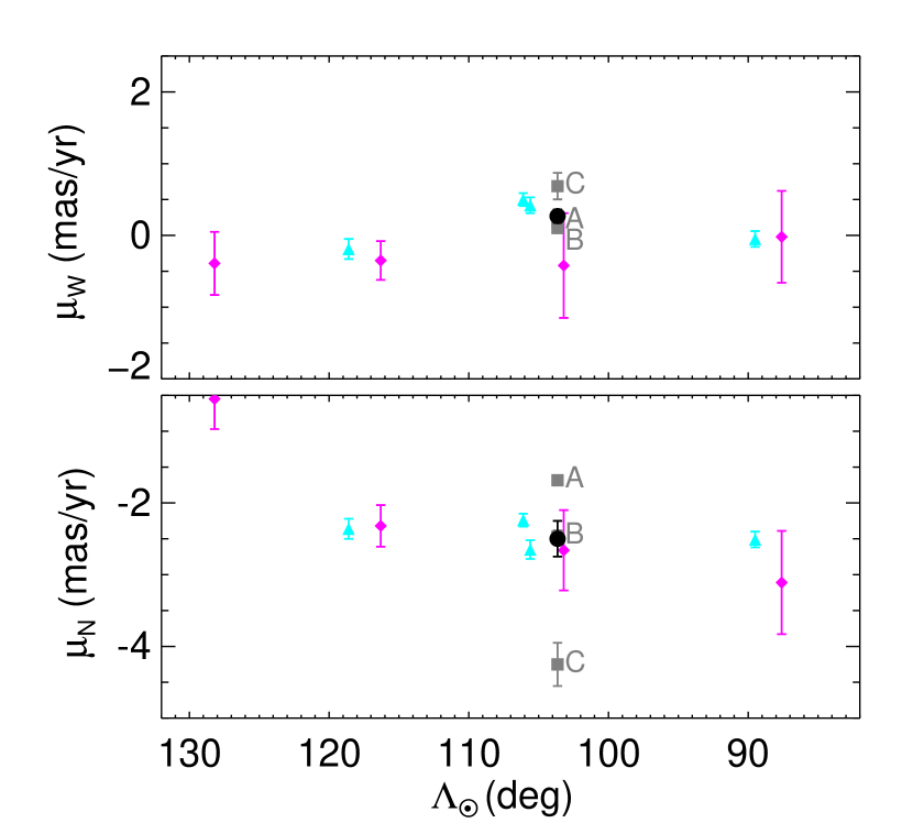
Figure 6.— Proper motions in the trailing arm, in the west (upper panel) and north (lower panel) directions, as a function of the Sgr latitude. Ground-based measurements from Carlin et al. (2012, magenta diamonds) and Koposov et al. (2013, cyan triangles) are shown for comparison. Our HST average for all identified Sgr stream stars in FIELD 1 (the combined A+B+C sample, as defined in Figure 2 and Table 6) is shown in black circle. Overall, the studies are in good agreement. The average PMs of our FIELD 1 A, B, and C samples are shown in grey squares.

4.2.2 Sgr dSph

The HST FIELD 2 is located at $(\Lambda_{\odot},B)=(-3.53^{\circ},4.65^{\circ})$. This places the Sgr stars in this field at $5.8^{\circ}$ from the Sgr dSph. In $N$-body simulations, bound material is found out to $\sim 8^{\circ}$ from the Sgr dSph (e.g., Law et al., 2005). Therefore, the Sgr stars identified in FIELD 2 give information primarily about the PM of the Sgr dSph itself, and less so about the kinematics of unbound stream material.

Several measurements of the PM of the Sgr dSph already exist in the literature, based on different kinds of data: Dinescu et al. (2005) used the ground-based Southern Proper Motion Catalog 3; Pryor et al. (2010) analyzed HST data of three fields; and Massari et al. (2013) analyzed HST data of a foreground globular cluster (NGC 6681), qualitatively similar to the case for our FIELD 2. Even though we are not the first to have used HST data to measure the PM of the Sgr dSph, our work does have several advantages over the previous studies. Pryor et al. (2010) used foreground Galactic stellar populations to set the astrometric reference frame, which requires assumptions about the PM kinematics of the foreground Galactic stellar population to obtain absolute PMs. Massari et al. (2013) instead used stationary background galaxies to set the astrometric reference frame as we do here, but they used only 5 background galaxies, which were fitted as point sources. By contrast, we used 24 background galaxies for our FIELD 2, and for each of these we build an individual template that takes the exact galaxy morphology into account.

All of the individual PM estimates, including the one presented here, pertain to different fields that do not coincide with the center-of-mass (COM) of the Sgr dSph. This implies that two effects need to be taken into account in any comparison. The first effect is that possible internal motions, such as rotation, could in principle contribute to the measurements for the different fields. However, this should not be a problem for the Sgr dSph, since this galaxy does not show any evidence of rotation (Peñarrubia et al., 2011; Frinchaboy et al., 2012). The second effect is that even in the absence of internal motions, one would not expect to measure the same PM for different fields, because of perspective effects. Depending on where one points in the Sgr dSph, different components of the 3D COM velocity vector project onto the local LOS, West, and North directions (van der Marel et al., 2002).

After correcting for viewing perspective following van der Marel & Guhathakurta (2008) and Massari et al. (2013), the following COM PM estimates are obtained for $(\mu_{W},\mu_{N})$: $(2.83\pm 0.20,-1.56\pm 0.20)\ \>{\rm mas}\,{\rm yr}^{-1}$ for Dinescu et al. (2005); $(2.37\pm 0.20,-1.63\pm 0.22)\ \>{\rm mas}\,{\rm yr}^{-1}$ for Pryor et al. (2010); $(2.56\pm 0.18,-1.29\pm 0.16)\ \>{\rm mas}\,{\rm yr}^{-1}$ for Massari et al. (2013). These measurements are mutually consistent, given the uncertainties, with a weighted average of $(2.59\pm 0.11,-1.49\pm 0.11)\ \>{\rm mas}\,{\rm yr}^{-1}$. The perspective-corrected estimate based on our HST FIELD 2 data is $(2.92\pm 0.07,-1.56\pm 0.11)\ \>{\rm mas}\,{\rm yr}^{-1}$.

The HST FIELD 2 result is very close to the value implied by the Dinescu et al. (2005) measurement, but the agreement with the Pryor et al. (2010) ($2.6\sigma$ different in the West direction) and the Massari et al. (2013) result ($1.9\sigma$ and $1.4\sigma$ different in the West and North directions, respectively) is less good. When comparing the HST FIELD 2 result to the weighted average of the previously published results, the difference is $(0.33\pm 0.13,-0.07\pm 0.16)\ \>{\rm mas}\,{\rm yr}^{-1}$. Such a residual can occur by chance in a two-dimensional Gaussian distribution at 4% probability. Hence, it is more likely that one or more of the measurements contain unquantified systematics. One way to account for this is to multiply all the error bars by a factor $1.8$, which makes the results statistically consistent ($\chi^{2}$ equal to the number of degrees of freedom). If we do this, and then take the weighted average of all four measurements, we obtain $(\mu_{W},\mu_{N})=(2.82\pm 0.11,-1.51\pm 0.14)\ \>{\rm mas}\,{\rm yr}^{-1}$. This is our current best estimate estimate of the COM PM of the Sgr dSph, based on all available measurements.

4.3. Preliminary Comparison to Model Proper Motions

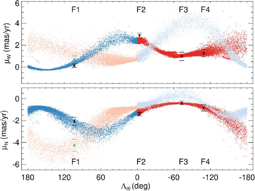
Figure 7.— Comparison of HST PM observations of $\mu_{W}$ (top) and $\mu_{N}$ (bottom) to the PMs of the $N$-body particles in the LM10 model, as function of the Sgr longitude $\Lambda_{\odot}$. The horizontal axis is chosen so that the Sgr dSph lies in the middle of each panel. The leading arm (red) extends to right from the dSph, while the trailing arm (blue) extends to the left (as is true for the view in equatorial coordinates; compare Figure 1). The primary wrap at each longitude (i.e., particles within $180^{\circ}$ in Sgr longitude from the dSph) are shown in bold colors. The secondary wrap at each longitude (i.e., particles that are between $180^{\circ}$–$360^{\circ}$ in Sgr longitude from the dSph) are shown with lighter colors. Particles that have an orbital phase that differs by more than $360^{\circ}$ from that of the dSph are not shown. A black solid dot with error bars shows for each HST field the average observed PM (from Table 6) for the stars identified as belonging to the primary wrap. This uses the A+B subsample averages for FIELD 1, 3, and 4. For FIELD 1 we also show as a green square the subsample C, identified as corresponding to the secondary (leading) wrap at that Sgr longitude. Horizontal bars above and below the data points indicate $\pm$ the PM dispersions estimated from the measurements (calculated as in Table 6, but now for the West and North directions separately).

For a preliminary assessment of what the new HST PM data may imply for our understanding of the Sgr stream, we qualitatively compare the data to the PM predictions of the existing $N$-body models of LM10 and Peñarrubia et al. (2010). Figure 7 shows the PMs $\mu_{W}$ and $\mu_{N}$ of the LM10 model’s $N$-body particles (colored) as function of the Sgr longitude $\Lambda_{\odot}$. The HST PM averages (black) are overplotted for comparison. Overall, the new measurements follow quite closely the predicted PM trend with Sgr longitude. This constitutes a remarkable success for the LM10 model. The model was fit only to distance and LOS velocity data for the stream, with no reference to PMs. So Figure 7 does not represent a fit to the data, but rather a successful verification of a prediction that was made a priori. Without further quantitative comparison, our PM results do not necessarily imply that the LM10 model is the only correct interpretation of the data, or that indeed the MW halo must be triaxial in the manner suggested by LM10. However, our new HST PM data certainly provide no immediate evidence for an obvious problem with the model.

Figure 7 shows that the biggest mismatch between the LM10 model and the HST PM data occurs for FIELD 2, which is sensitive primarily to the PM of the Sgr dSph. In the LM10 model, the best-fit Galactocentric velocity for the Sgr dSph was found to be $(V_{X},V_{Y},V_{Z})=(230,-35,195)\ \>{\rm km}\,{\rm s}^{-1}$. With the same assumptions made by LM10 for the solar circular velocity ($V_{\rm circ}=220\ \>{\rm km}\,{\rm s}^{-1}$) and Sgr dSph distance ($D=28\ \>{\rm kpc}$), the COM PM predicted by the model is $(\mu_{W},\mu_{N})=(2.45,-1.30)\ \>{\rm mas}\,{\rm yr}^{-1}$. This is in the same direction on the sky as the best-estimate PM derived in Section 4.2.2, but lower in amplitude by about 14%. This discrepancy may be resolved by one or a combination of several things.

Carlin et al. (2012) constructed variations to the $N$-body models of LM10, in which $V_{\rm circ}$ was treated as a free parameter. They showed that when $V_{\rm circ}$ is increased from the canonical $220\ \>{\rm km}\,{\rm s}^{-1}$ to a value as high as $264\ \>{\rm km}\,{\rm s}^{-1}$, then the best-fit PM of the Sgr dSph (see their Figure 19) is $(\mu_{W},\mu_{N})=(2.78,-1.55)\ \>{\rm mas}\,{\rm yr}^{-1}$. This is in excellent agreement with our best estimate estimate COM PM $(\mu_{W},\mu_{N})=(2.82\pm 0.11,-1.51\pm 0.14)\ \>{\rm mas}\,{\rm yr}^{-1}$, based on all available PM measurements. However, it is not obvious that such a large $V_{\rm circ}$ is plausible in the context of other astronomical knowledge. The azimuthal velocity of the sun in this model, taking into account also the $12\ \>{\rm km}\,{\rm s}^{-1}$ solar peculiar azimuthal velocity, is $v_{\phi,\odot}=276\ \>{\rm km}\,{\rm s}^{-1}$. Bovy et al. (2012) recently found from a detailed study of APOGEE data that $v_{\phi,\odot}=242^{+10}_{-3}\ \>{\rm km}\,{\rm s}^{-1}$. Also, Carlin et al. (2012) found from fitting their trailing arm PM data a best fit value $V_{\rm circ}=232\pm 14\ \>{\rm km}\,{\rm s}^{-1}$. So while there is now growing consensus that the solar velocity may be larger than previously believed (and adopted by LM10), its value may not be quite as large as needed to bring the $N$-body models in agreement with the Sgr dSph PM measurements.

Another change to the LM10 model that would bring its PM predictions closer to the measurements, would be to decrease the distance of the Sgr dSph. For example, excellent agreement would be obtained if the Sgr dSph is in fact at $D\approx 24\ \>{\rm kpc}$, i.e., 14% closer than adopted by LM10 based on the Siegel et al. (2011) HST observations of the Sgr core. This effect will be demonstrated below when we compare our PM measurements with the $N$-body models of Peñarrubia et al. (2010). A lower distance would be consistent with some values that have been proposed and used previously in the literature (e.g., Law et al., 2005; Belokurov et al., 2006).

Possibly the LM10 adopted solar velocity is somewhat too low and the adopted Sgr dSph distance is somewhat too high. Or alternatively, other effects may contribute. This could be explored explicitly through future $N$-body models that are specifically tailored to fit the new HST PM data.

There is also a (smaller) mismatch between the PM data and the LM10 model for the leading stream stars in FIELD 1 (green data points in Figure 7). In particular, their observed $\mu_{W}$ component is somewhat smaller in the data than in the models. This mismatch is also evident in Figure 2c. It is likely that an understanding of this mismatch will provide improved insights into stream models.

The measured dispersions for the fields are indicated with horizontal bars above and below the data points in Figure 7. By-and-large, these dispersions are of similar size as the PM spreads for the LM10 model particles (with the possible exception of FIELD 3). This suggests that much of the spreads in our PM measurements are reflective of intrinsic scatter between individual stream star PMs, and are not merely due to PM measurement errors. In turn, this implies that our PM uncertainties are small enough to be able to probe the internal kinematics of the stream, and not merely its bulk motion. It is intriguing in this context that in three of our four fields, we find indications that two distinct kinematical components (A and B) may exist within the same arm and wrap of the stream. This is not predicted by the LM10 model, and may tell us something new about the structure of the Sgr dSph prior to its disruption. Possibly related, it is of interest to note that there does also exist a spatial bifurcation in the leading arm of the stream (Belokurov et al., 2006) which is not currently well understood.

We have also compared our PM measurements with the $N$-body models of Peñarrubia et al. (2010) in a similar manner as we did for LM10. The result is shown in Figure 8. Again, the variation of the HST PM measurements with Sgr longitude shows good overall qualitative agreement with the $N$-body model predictions. This provides yet another important consistency check on our PM measurements. It also confirms most of what we already concluded from the comparison with the LM10 model. However, there are two differences between the LM10 and Peñarrubia et al. (2010) data-model comparisons that are worth noting. On the one hand, our average PM for FIELD 2 is better matched by the Peñarrubia et al. model than by the LM10 model. This is probably because Peñarrubia et al. (2010) used a distance to the Sgr dSph of only $D=25\>{\rm kpc}$ (smaller than the $D=28\>{\rm kpc}$ adopted by LM10), but with a similar Solar motion. On the other hand, the agreement between the PM data and the $N$-body predictions for the leading stream stars in FIELD 1 is significantly worse for the Peñarrubia et al. (2010) model than for the LM10 model.

In Paper II we quantitatively compare the new HST data to Sgr stream models. We use this comparison to shed new light on topics such as the structure and distance of the Sgr stream, the solar velocity in the MW disk, and the shape of the MW’s dark halo.

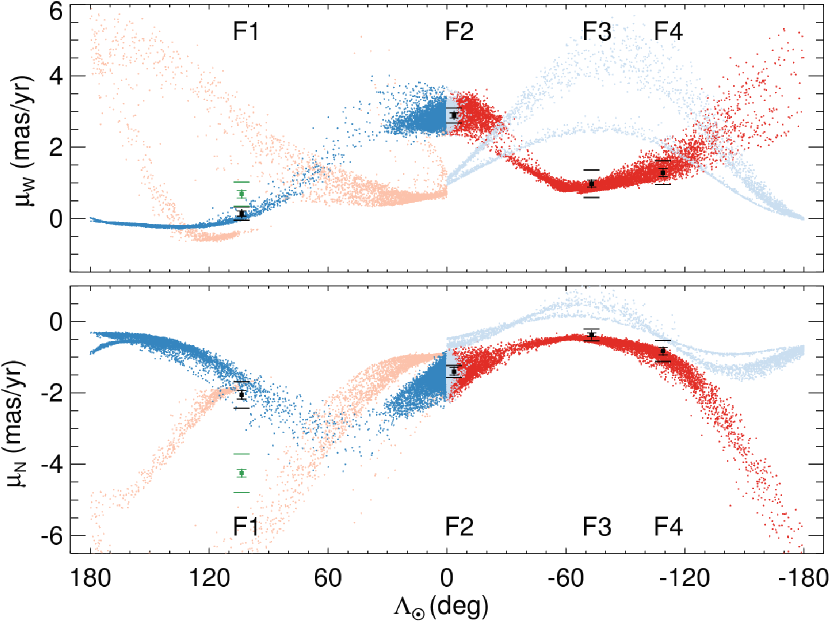
Figure 8.— Same as Figure 7 but comparison with $N$-body models of Peñarrubia et al. (2010).

5. Summary and Conclusions

The Sgr stream is an ideal target for probing in detail several important topics, including the tidal disruption of dwarf galaxies, the hierarchical buildup of stellar halos, the shape, orientation and mass of the MW’s dark halo, and the velocity of the Sun in the MW disk. To be able to better use the stream to address these issues, we have presented an HST study of the variation in stellar PMs along the stream.

We observed four fields along the Sgr stream: one field in the trailing arm, one field near the Sgr dSph tidal radius, and two fields in the leading arm. These fields span a range of more than 200 degrees along the Sgr stream. We combined the results with existing archival data to yield time baselines of 6–9 years. From the data we determined two-band photometry and absolute PMs for individual stars in these fields. We used distant background-galaxies to define a stationary reference frame. Our sophisticated PM measurement techniques have been previously developed, tested, and applied in the context of other Local Group projects. Any residual systematic PM errors are expected to be below the level of the random measurement errors.

By combining CMD and PM information it is possible to identify individual Sgr stream stars in each of the fields, and to reliably reject most foreground and background objects. This yields for the first time accurate individual (as opposed to average) PM measurements of stars in the stream. This allows separation of different kinematical components and wraps within the stream. For example, in our trailing-arm field, the PMs allow us to kinematically separate ten trailing-arm stars from three leading-arm stars. These leading-arm stars are a full revolution ahead in their orbit around the MW compared to the trailing-arm stars.

We compared our results to the small body of existing average PM measurements for the Sgr stream and dSph. Our results are broadly consistent with the existing work, but have higher accuracy. Moreover, our results provide the first PM measurements in the leading arm of the stream, which can help constrain MW halo properties over a wider range of radii.

For a preliminary assessment of what the new HST PM data may imply for our understanding of the Sgr stream, we qualitatively compared the data to the PM predictions of the $N$-body models of LM10 and Peñarrubia et al. (2010). Overall, our measurements follow quite closely the predicted PM trends with Sgr longitude. Also, the measured PM dispersions are broadly comparable to those in the models. This provides a successful consistency check on the PM measurements. It also constitutes a remarkable success for the $N$-body models, which were fit only to distance and LOS velocity data for the stream, with no reference to PMs.

Nonetheless, there are some areas of mismatch between the models and our PM data, as discussed in Section 4.3. Also, in three of our fields we find indications that two distinct kinematical components (A and B) may exist within the same arm and wrap of the stream. This may tell us something new about the structure of the Sgr dSph prior to its disruption. In Paper II we will quantitatively compare the new HST PM data to Sgr stream models, and we use this comparison to shed new light on topics such as the structure and distance or the Sgr stream, the solar velocity in the MW disk, and the shape of the MW?s dark halo.

The observational techniques presented here will be equally useful for the study of other structures in the MW halo. For example, we have an ongoing HST observing program (GO-13443, PI: R. P. van der Marel) to determine PMs along the Orphan Stream. This will better constrain its orbit, and may allow identification of its progenitor (if it is not already entirely disrupted). When observations from different streams are combined, it should also be possible to constrain more tightly the shape and mass of the MW dark halo. We also have an ongoing HST archival legacy program (AR-13272, PI: R. P. van der Marel), to determine the PMs of metal-poor halo stars in random pointings multiply-imaged by HST. This will not only constrain the velocity dispersion anisotropy of the dynamically hot halo, buy may also lead to identification of new streams if cold structures are found to exist in PM space.

Appendix A A. PSF Kernels

To determine accurate PMs, it is important to account for PSF differences between epochs. Specifically, it is known that a subtle change in the ACS/WFC PSF was introduced by the Space Shuttle Servicing Mission 4. We account for this through application of a 7$\times$7 pixel convolution kernel to one of the two epochs. As discussed in Section 2.3, our FIELDS 1, 3, and 4 are too sparse to reliably derive these kernels from the actual point sources observed in these fields. So for these fields we used an alternative method based on library PSFs.

We first created two sets of simulated images, representing the first and second epoch, by injecting 1,000 stars with random brightness ($S/N>100$) in random locations. The background characteristics of the simulated images, such as the mean and standard deviation, were chosen to follow those of our observed images. Position-dependent library PSFs (Anderson & King, 2006) constructed separately for the pre- and post-SM4 period were used when injecting stars into the simulated first- and second-epoch images, respectively. Using these stars in the two sets of simulated images, we obtained a kernel that accounts for the differences between the pre- and post-SM4 PSFs, similarly to our analysis of the FIELD 2 data (see Section 2.3). We did this separately for each of the F775W and F814W filters. These kernels were then applied to the templates when fitting a star or galaxy in the second-epoch images for FIELDS 1, 3, and 4.

Appendix B B. Absolute Proper Motion of the Globular Cluster NGC 6652

In the course of our PM analysis of FIELD 2, we have also obtained the absolute PM of the globular cluster NGC 6652:

$$\mu_{\rm NGC6652}=(\mu_{W},\mu_{N})=(5.66\pm 0.07,-4.45\pm 0.10)\ {\rm mas\ yr}^{-1}.$$ (B1)

To determine the implied Galactocentric motion, we adopt a Cartesian Galactocentric coordinate system ($X,Y,Z$), with the origin at the Galactic Center, the $X$-axis pointing in the direction from the Sun to the Galactic Center, the $Y$-axis pointing in the direction of the Sun’s Galactic rotation, and the $Z$-axis pointing towards the Galactic North Pole. The position and velocity of an object in this frame can be determined from the observed sky position, distance, line-of-sight velocity, and proper motion.

For the distance $R_{0}$ of the Sun from the Galactic Center and the circular velocity of the local standard of rest (LSR), we adopt the recent values of McMillan (2011): $R_{0}=8.29\pm 0.16\ \>{\rm kpc}$ and $V_{0}=239\pm 5\ \>{\rm km}\,{\rm s}^{-1}$. For the solar peculiar velocity with respect to the LSR we adopt the estimates of Schönrich et al. (2010): $(U_{\rm pec},V_{\rm pec},W_{\rm pec})=(11.10,12.24,7.25)\ \>{\rm km}\,{\rm s}^{-1}$ with uncertainties of $(1.23,2.05,0.62)\ \>{\rm km}\,{\rm s}^{-1}$.

The distance to NGC 6652 is $10.5\pm 0.5$ kpc (Chaboyer, Sarajedini, & Armandroff, 2000), and the heliocentric line-of-sight velocity is $-111.7\pm 5.8\ \>{\rm km}\,{\rm s}^{-1}$ (Harris, 1996, 2010 edition). These imply a Galactocentric $(X,Y,Z)$ position

$${\vec{r}}=(2.0,0.3,-2.1)\ \>{\rm kpc},$$ (B2)

and a Galactocentric velocity vector

$${\vec{v}}=(-58.0\pm 6.2,-70.6\pm 16.4,187.4\pm 8.2)\ \>{\rm km}\,{\rm s}^{-1}.$$ (B3)

The corresponding Galactocentric radial and tangential velocities are

$$(V_{\rm rad},V_{\rm tan})=(-181.0\pm 7.2,103.4\pm 31.9)\ \>{\rm km}\,{\rm s}^{-1},$$ (B4)

and the observed total velocity of NGC 6652 with respect to the MW is

$$v\equiv|{\vec{v}}|=208.5\pm 11.8\ \>{\rm km}\,{\rm s}^{-1}.$$ (B5)

The listed uncertainties above are obtained from a Monte-Carlo scheme that propagates all observational distance and velocity uncertainties and their correlations, including those for the Sun.

References

- Abraham et al. (2004) Abraham, R. G., Glazebrook, K., McCarthy, P. J., et al. 2004, AJ, 127, 2455
- Anderson & King (2006) Anderson J., & King, I. R. 2006, ACS/ISR 2006-01, PSFs, Photometry, and Astrometry for the ACS/WFC (Baltimore: STScI) (AK06)
- Anderson & Bedin (2010) Anderson, J. & Bedin, L. R. 2010, PASP, 122, 1035
- Belokurov et al. (2006) Belokurov, V., Zucker, D. B., Evans, N. W., et al. 2006, ApJ, 642, L137
- Belokurov et al. (2014) Belokurov, V., Koposov, S. E., Evans, N. W., et al. 2014, MNRAS, 437, 116
- Bertin & Arnouts (1996) Bertin, E., & Arnouts, S. 1996, A&AS, 117, 393
- Besla et al. (2010) Besla, G., Kallivayalil, N., Hernquist, L., et al. 2010, ApJ, 721, 97
- Bovy et al. (2012) Bovy, J., Allende Prieto, C., Beers, T. C., et al. 2012, ApJ, 759, 131
- Carlin et al. (2012) Carlin, J. L., Majewski, S. R., Casetti-Dinescu, D. I., et al. 2012, ApJ, 744, 25
- Casey et al. (2013) Casey, A. R., Da Costa, G., Keller, S. C., & Maunder, E. 2013, ApJ, 764, 39
- Chaboyer, Sarajedini, & Armandroff (2000) Chaboyer, B., Sarajedini, A., & Armandroff, T. E. 2000, AJ, 120, 3102
- Chou et al. (2010) Chou, M. -Y., Cunha, K., Majewski, S. R., et al. 2010, ApJ, 708, 1290
- Deason et al. (2013) Deason, A. J., van der Marel, R. P., Guhathakurta, P., Sohn, S. T., & Brown, T. M. 2013, ApJ, 766, 24
- Deason et al. (2014) Deason, A. J., Belokurov, V., Koposov, S. E., & Rockosi, C. M. 2014, ApJ, 787, 30
- Deg & Widrow (2013) Deg, N., & Widrow, K. 2013, MNRAS, 428, 912
- Dinescu et al. (2005) Dinescu, D. I., Girard, T. M., van Altena, W. F., & López, C. E. 2005, ApJ, 618, 25
- Dotter et al. (2008) Dotter, A., Chaboyer, B., Jevremović, D., et al. 2008, ApJS, 178, 89
- Efron & Tibshirani (1993) Efron, B., & Tibshirani, R. 1993, An Introduction to the Bootstrap (Chapman & Hall/CRC)
- Fellhauer et al. (2006) Fellhauer, M., Belokurov, V., Evans, N. W., et al. 2006, ApJ, 651, 167
- Ferguson et al. (2002) Ferguson, A. M. N., Irwin, M. J., Ibata, R. A., Lewis, G. F., & Tanvir, N. R. 2002, AJ, 124, 1452
- Frinchaboy et al. (2012) Frinchaboy, P. M., Majewski, S. R., Muñoz, R. R., et al. 2012, ApJ, 756, 74
- Harris (1996) Harris, W. E. 1996, AJ, 112, 1487
- Helmi (2004) Helmi, A. 2004, ApJ, 610, L97
- Helmi (2008) Helmi, A. 2008, ARA&A, 15, 145
- Ibata et al. (1994) Ibata, R. A., Gilmore, G., & Irwin, M. J. 1994, Nature, 370, 194
- Ibata et al. (2001) Ibata, R., Lewis, G. F., Irwin, M., Totten, E., & Quinn, T. 2001, ApJ, 551, 294
- Ibata et al. (2013) Ibata, R., Lewis, G. F., Martin, N. F., et al. 2013, ApJ, 765, L15
- Johnston et al. (2005) Johnston, K. V., Law, D. R., & Majewski, S. R. 2005, ApJ, 619, 800
- Kallivayalil et al. (2013) Kallivayalil, N., van der Marel, R. P., Besla, G., Anderson, J., & Alcock, C. 2013, ApJ, 764, 161
- Koposov et al. (2012) Koposov, S. E., Belokurov, V., Evans, N. W., et al. 2012, ApJ, 750, 80
- Koposov et al. (2013) Koposov, S. E., Belokurov, V., & Evans, N. W. 2013, ApJ, 766, 79
- Law et al. (2005) Law, D. R., Johnston, K., V., & Majewski, S. R. 2005, ApJ, 619, 807
- Law et al. (2009) Law, D. R., Majewski, S. R.,& Johnston, K., V. 2009, ApJ, 703, L67
- Law & Majewski (2010) Law, D. R., & Majewski, S. R. 2010, ApJ, 714, 229 (LM10)
- Majewski et al. (1999) Majewski, S. R., Siegel, M. H., Kunkel, W. E., et al. 1999, AJ, 118, 1709
- Majewski et al. (2003) Majewski, S. R., Skrutskie, M. F., Weinberg, M. D., & Ostheimer J . C. 2003, ApJ, 599, 1082
- Majewski et al. (2004) Majewski, S. R., Kunkel, W. E., Law, D. R., et al. 2004, AJ, 128, 245
- Martínez-Delgado et al. (2001) Martínez-Delgado, D., Aparicio, A., Gómez-Flechoso, M. Á, & Carrera, R. 2001, ApJ, 549, L199
- Martínez-Delgado et al. (2002) Martínez-Delgado, D., Zinn, R., Carrera, R., & Gallart, C. 2002, ApJ, 573, L19
- Martínez-Delgado et al. (2007) Martínez-Delgado, D., Peñarrubia, J., Jurić, M., Alfaro, E. J., & Ivezić, Z. 2007, ApJ, 660, 1264
- Martínez-Delgado et al. (2012) Martínez-Delgado, D., Romanowsky, A. J., Gabany, R. J., et al. 2012, ApJ, 748, L24
- Massari et al. (2013) Massari, D., Bellini, A., Ferraro, F. R., et al. 2013, ApJ, 779, 81
- Mateo et al. (1998) Mateo, M., Olszewski, E. W., & Morrison, H. L. 1998, ApJ, 508, L55
- McMillan (2011) McMillan, P. J. 2011, MNRAS, 414, 2446
- Monaco et al. (2007) Monaco, L., Bellazini, M., Bonifacio, P., et al. 2007, A&A, 464, 201
- Nidever et al. (2008) Nidever, D. L., Majewski, S. R., & Burton, W. B. 2008, ApJ, 679, 432
- Odenkirchen et al. (2009) Odenkirchen, M., Grebel, E. K., Kayser, A., Rix, H.-W., & Dehnen, W. 2009, AJ, 137, 3378
- Peñarrubia et al. (2010) Peñarrubia, J., Belokurov, V., Evans, N. W., et al. 2010, MNRAS, 408, L26
- Peñarrubia et al. (2011) Peñarrubia, J., Zucker, D. B., Irwin, M. J., et al. 2011, ApJ, 727, L2
- Pryor et al. (2010) Pryor, C., Piatek, S., & Olszewski, E. W. 2010, AJ, 139, 839
- Robin et al. (2003) Robin, A. C., Reylé, C., Derrière, S., & Picaud, S. 2003, A&A, 409, 523
- Robin et al. (2014) Robin, A. C., Reylé, C., Fliri, J., et al. 2014, A&A, 569, 13
- Sarajedini et al. (2007) Sarajedini, A., Bedin, L. R., Chaboyer, B., et al. 2007, AJ, 133, 1658
- Schlafly & Finkbeiner (2011) Schlafly, E. F., & Finkbeiner, D. P. 2011, ApJ, 737, 103
- Schlegel, Finkbeiner, & Davis (1998) Schlegel, D. J., Finkbeiner, D. P., & Davis, M. 1998, ApJ, 500, 525
- Schönrich et al. (2010) Schönrich, R., Binney, J., & Dehnen, W. 2010, MNRAS, 403, 1829
- Siegel et al. (2007) Siegel, M. H., Dotter, A., Majewski, S. R., et al. 2007, ApJ, 667, L57
- Siegel et al. (2011) Siegel, M. H., Majewski, S. R., Law, D. R., et al. 2011, ApJ, 743, 20
- Sirianni et al. (2005) Sirianni, M., Jee, M. J., Benítez, N., et al. 2005, PASP, 117, 1049
- Slater et al. (2013) Slater, C. T., Bell, E. F., Schlafly, E. F., et al. 2013, ApJ, 762, 6
- Sohn et al. (2010) Sohn, S. T., Anderson, J., & van der Marel, R. P. 2010, in 2010 Space Telescope Science Institute Calibration Workshop - Hubble after SM4. Preparing JWST, ed. S. Deustua, & C. Oliveira (Baltimore, MD: STScI), 35
- Sohn et al. (2012) Sohn, S. T., Anderson, J., & van der Marel, R. P. 2012, ApJ, 753, 7
- Sohn et al. (2013) Sohn, S. T., Besla, G., van der Marel, R. P, et al. 2013, ApJ, 768, 139
- van der Marel et al. (2002) van der Marel, R. P., Alves, D. R., Hardy, E., & Suntzeff, N. B. 2002, AJ, 124, 2639
- van der Marel & Guhathakurta (2008) van der Marel, R. P., & Guhathakurta, P. 2008, ApJ, 678, 187
- van der Marel et al. (2013) van der Marel, R. P., Anderson, J., Bellini, A., et al. 2013, in ”Structure and Dynamics of Disk Galaxies”, M. S. Seigar & P. Treuthardy, eds., ASP Conference Series (arXiv:1309.2014)
- Vera-Ciro & Helmi (2013) Vera-Ciro, C., & Helmi, A. 2013, ApJ, 773, L4