On the NP-completeness of the Hartree-Fock method for translationally invariant systems

Abstract

The self-consistent field method utilized for solving the Hartree-Fock (HF) problem and the closely related Kohn-Sham problem, is typically thought of as one of the cheapest methods available to quantum chemists. This intuition has been developed from the numerous applications of the self-consistent field method to a large variety of molecular systems. However, as characterized by its worst-case behavior, the HF problem is NP-complete. In this work, we map out boundaries of the NP-completeness by investigating restricted instances of HF. We have constructed two new NP-complete variants of the problem. The first is a set of Hamiltonians whose translationally invariant Hartree-Fock solutions are trivial, but whose broken symmetry solutions are NP-complete. Second, we demonstrate how to embed instances of spin glasses into translationally invariant Hartree-Fock instances and provide a numerical example. These findings are the first steps towards understanding in which cases the self-consistent field method is computationally feasible and when it is not.

I Introduction

The Hartree-Fock (HF) methodHartree (1928); Fock (1930) is one of the most important quantum chemistry techniques as it provides the mathematical setting for the chemist’s notion of molecular orbitals widely used in organic chemistry. While this method is known to be a weak approximation in many cases (e.g. in strongly correlated systems such as transition metal complexes, at non-equilibrium geometries, etc.), it serves also the basis for more sophisticated (post-Hartree-Fock) algorithms which improve the mean-field wave function obtained. Moreover, the self-consistent field (SCF) methodology used to finding the Hartree-Fock ground-state solution is also applied to solve Kohn-Sham density functional theory.

For practitioners of quantum chemistry, the runtime of the Hartree-Fock algorithm method is often dominated by the time needed to form and diagonalize the Fock matrix at each iteration leading to a third order scaling in the size of the basis set. Linear scaling methods Goedecker (1999) avoid diagonalization entirely and rely on localization properties of the system that may not generally exist in three-dimensional systems. Regardless, these methods have yet to mature to the point where they can supplant ordinary implementations. Typical approaches to improving SCF are based on direct inversion of the iterative subspacePulay (1980), level shiftingSaunders and Hillier (1973), quadratically convergent Newton-Raphson techniques Bacskay (1981), semidefinite programmingVeeraraghavan and Mazziotti (2014a); *Mazziotti14b or varying fractional occupation numbersRabuck and Scuseria (1999) among many other approaches. The success of these approaches depends on the specific situation and the parameters chosen (e.g. the size of the iterative subspace) and often work well in combination. The success of these various methods has led to attempts to build black-box SCF procedures.Thøgersen et al. (2004); Kudin, Scuseria, and Cancès (2002)

Unfortunately, these methods cannot work efficiently in all cases since it was shown that Hartree-Fock is NP-complete.Schuch and Verstraete (2009); Whitfield, Love, and Aspuru-Guzik (2013) In this article, we expand upon the previous findings using translational symmetry to examine easy and hard instances when enforcing or breaking the symmetry of the underlying Hamiltonian. Let us note here that the translational invariance of the $N$-body Hamiltonian does not imply that the Hartree-Fock state also carries this symmetry.Overhauser (1960) In general, when variational Ansätze give lowest energy state without the same symmetry as the true wave function, this is called a symmetry broken solution. The choice between the variational state with correct symmetries or the symmetry broken state is often referred to as Löwdin’s dilemma.Lykos and Pratt (1963) Taking this into account, we will give examples of 1) translationally invariant HF systems that are NP-complete in the symmetry-broken space but are trivially simple when enforcing symmetry and 2) translationally invariant HF systems that are NP-complete also when the symmetry is enforced. We will prove these NP-completeness results by embedding spin glass models into HF instances.

I.1 Hartree-Fock Theory

A two-body Hamiltonian over $M$ sites has the general form

$$H= H_{1}+H_{2}$$

$$= \sum_{ij}h_{ij}a^{\dagger}_{i}a^{\phantom{\dagger}}_{j}+\frac{1}{2}\sum_{ijkl}h_{ijkl}a^{\dagger}_{i}a^{\dagger}_{j}a^{\phantom{\dagger}}_{k}a^{\phantom{\dagger}}_{l}.$$ (1)

The goal of Hartree-Fock is to minimize the energy within the set $F_{1}$ of single Slater determinants

$$E_{HF} =\min_{\Psi\in F_{1}}\langle\Psi|H|\Psi\rangle\,.$$ (2)

The single Slater determinant corresponding to the minimal value of $E_{HF}$ is called the Hartree-Fock state:

$$|\Psi_{HF}\rangle=b_{1}^{\dagger}b_{2}^{\dagger}\cdots b_{N}^{\dagger}|vac\rangle.$$ (3)

In this expression

$$b_{i}^{\dagger}=\sum_{j}a^{\dagger}_{j}C_{ji}$$ (4)

corresponds to the creation operators of the molecular orbitals, $\psi_{i}(x)=\sum_{j}\phi_{j}(x)C_{ji}$, while $a^{\dagger}_{j}$ and $a_{j}$ are creation and annihilation operators in the given atomic orbital basis, $\phi_{i}(x)$. The creation/annihilation operators must satisfy the canonical anticommutation relations

$$[a_{i},a_{j}^{\dagger}]_{+}=\langle\phi_{i}|\phi_{j}\rangle\mathbbmss{1}\,,\;[a_{i},a_{j}]_{+}=0,$$ (5)

$$[b_{i},b^{\dagger}_{j}]=\delta_{i,j}\mathbbmss{1}\,,\;\;\;\;[b_{i},b_{j}]_{+}=0.$$ (6)

In other words, the orbital-rotation matrix $C$, which connects the atomic and molecular orbitals, is chosen in such a way that Eq. (6) is satisfied and the corresponding state of Eq. (3) is the Slater determinant that minimizes the energy. Let us note that if the atomic orbitals are orthogonal, $C$ will be unitary.

The charge density operator is defined as

$$P_{pq}=\sum_{i}^{occ}C^{\phantom{*}}_{pi}C^{*}_{qi},$$ (7)

where the summation goes only over the occupied orbitals. One can expand Eq. (2) using this operator as

$$E_{HF} =\min_{P}\sum_{pq}P_{qp}h_{pq}+\frac{1}{2}\sum_{pqrs}P_{qp}P_{sr}(h_{prsq}-h_{prqs})$$

$$=\min_{P}\frac{1}{2}Tr\left[P\left(F+H_{1}\right)\right],$$ (8)

where $F=F(P)=H_{1}+G(P)$ is the Fock operator and $G_{pq}=G(P)_{pq}=\sum_{rs}P_{sr}(h_{prsq}-h_{prqs})$ is the mean-field potential, which approximates the two-body interaction. Since the two-electron integrals frequently appear in pairs, we define $A_{pqrs}=h_{pqrs}-h_{pqsr}$ as the antisymmetric integral.

I.2 Translationally invariant fermionic systems

In this article, we focus our attention on translationally invariant fermionic Hamiltonians and examine two types of Hamiltonians whose Hartree-Fock problems are both NP-complete. Hamiltonians with translation symmetry appear in many areas of chemistry and physics, e.g., when modeling the electronic structure of solidsAshcroft and Mermin (1976), conjugated polymersStevens (1990) or fermionic atoms in optical lattices.Bloch, Dalibard, and Zwerger (2008)

The typical scenario has $L^{D}$ lattice sites each with $n_{s}$ orbitals per site (e.g., $n_{s}=2$ could represent the two spin orbital associated with a spatial orbital), and then translational invariance is imposed on the sites and, finally, boundary conditions are applied in each of the $D$ dimensions. To denote translational invariance over multi-orbital sites requires an intra-site label $o_{i}$ for the $i$th site. In this notation, translational symmetry means $h_{s_{1}s_{2}}^{o_{1}o_{2}}=h_{(s_{1}+1)(s_{2}+1)}^{o_{1}o_{2}}$ and $h_{s_{1}s_{2}s_{3}s_{4}}^{o_{1}o_{2}o_{3}o_{4}}=h_{(s_{1}+1)(s_{2}+1)(s_{3}+1)(s_{4}+1)}^{o_{1}o_{2}o_{3}o_{4}}$.

For simplicity, we’ll consider spinless fermions ($n_{s}=1$) and take periodic boundary conditions, i.e., in our examples the Hamiltonians will have the symmetry property

$$h_{(i+1)(j+1)}=h_{ij}\;\;\text{and}\;\;h_{(i+1)(j+1)(k+1)(l+1)}=h_{ijkl},$$

where indices are used cyclically ($k+M=k$). Since the system is translationally invariant, the Fourier transformed modes will often be used; these are defined over $M$ sites as

$$\mathcal{F}[a]_{m} = \hat{a}_{m}=\frac{1}{\sqrt{M}}\sum_{x}e^{-2\pi imx/M}a_{x}\,,$$ (9)

$$\mathcal{F}^{-1}[\hat{a}]_{x} = a_{x}=\frac{1}{\sqrt{M}}\sum_{m}e^{2\pi imx/M}\hat{a}_{m}\,.$$ (10)

I.3 NP-complete spin glasses

In this work, we will be proving the NP-completeness of various Hartree-Fock problems by showing that classical Ising spin glass problems can be embedded into them. Deciding if the ground state energy is below a certain value for the Ising Hamiltonian,

$$H_{I}=-\sum_{ij}J_{ij}S_{i}S_{j},$$ (11)

was shown to be NP-completeBarahona (1982) for $J_{ij}\in\{+1,-1,0\}$ with nearest neighbor connectivity on an $L\times L\times 2$ graph. Further investigations showed the problem for spin systems with non-planar connectivity are still NP-complete. By introducing one-body terms, even models on planar graphs were shown to be NP completeIstrail (2000); and recently various results on three-body and higher interactions have also been published.Whitfield, Faccin, and Biamonte ; Lucas (2014)

II NP-complete Hartree-Fock instances with trivial translationally invariant Slater determinants

Consider a $L\times L\times 2$ lattice, whose sites are labeled by the integers $1,\ldots,2L^{2}$ according to some ordering. Furthermore, consider an arbitrary but fixed Ising model on this lattice with couplings $J_{ij}\in\{-1,0,+1\}$ when $i$ and $j$ label neighboring sites and $J_{ij}=0$ otherwise. As discussed in Section I.3, the ground state problem for this set of models is NP-complete.

In the following, we will define a set of translation-invariant fermionic models whose ground state problem can be mapped to the above Ising ground state problem, and vice versa. Moreover, our mapping will ensure that for each instance at least one of the ground states is a Slater determinant corresponding to the solution of the given spin glass. This will imply that the corresponding Hartree-Fock energy decision problem is NP-complete. Interestingly, it will also turn out that by restricting the trial states to translationally invariant Slater determinants, the restricted HF problem becomes trivial and thus no longer NP-complete.

We will embed an arbitrary instance of the NP-complete Ising problem on the $L\times L\times 2$ lattice to a HF problem, by constructing a fermionic embedding Hamiltonian over $M=2(2L^{2})$ modes with the following form:

$$H= \sum^{M}_{i=1}\sum^{M}_{j=1}J_{ij}\left(\hat{a}^{\dagger}_{i}\hat{a}^{\phantom{\dagger}}_{M-i}+\hat{a}^{\dagger}_{M-i}\hat{a}^{\phantom{\dagger}}_{i}\right)\left(\hat{a}^{\dagger}_{M-j}\hat{a}^{\phantom{\dagger}}_{j}+\hat{a}^{\dagger}_{j}\hat{a}^{\phantom{\dagger}}_{M-j}\right),$$ (12)

where $J_{ij}$ is a fixed set of nearest neighbor couplings defining the original problem and the $\hat{a}_{k}$’s denote the Fourier transformed fermion operators, as defined in Eq. (10). Since an interaction term of form $\hat{a}^{\dagger}_{k_{1}}\hat{a}^{\phantom{\dagger}}_{k_{2}}\hat{a}^{\dagger}_{k_{3}}\hat{a}^{\phantom{\dagger}}_{k_{4}}+h.c.$ is translation-invariant if and only if

$$k_{1}+k_{3}-(k_{2}+k_{4})=0\mod M,$$ (13)

the Hamiltonian is translationally invariant.

Following the standard methods of Hartree-Fock, we will assume a fixed particle number. In the present case it will be half filling, i.e., the number of electrons in the system will be half the number of orbitals. However, we will work in the second quantized formalism (not constraining the number of particles) and only apply the half filling condition in the course of the proof.

II.1 Translationally invariant Slater determinants

Let us consider first the case when we restrict the HF problem of Eq. (12) to translationally invariant trial functions. If $|\Psi\rangle$ is a Slater determinant, we have by Wick’s theorem Wick (1950); Shavitt and Bartlett (2009)

$$\langle\Psi|\hat{a}^{\dagger}_{k_{1}}\hat{a}^{\phantom{\dagger}}_{k_{2}}\hat{a}^{\dagger}_{k_{3}}\hat{a}^{\phantom{\dagger}}_{k_{4}}|\Psi\rangle =\langle\Psi|\hat{a}^{\dagger}_{k_{1}}\hat{a}^{\phantom{\dagger}}_{k_{2}}|\Psi\rangle\langle\Psi|\hat{a}^{\dagger}_{k_{3}}\hat{a}^{\phantom{\dagger}}_{k_{4}}|\Psi\rangle$$

$$-\langle\Psi|\hat{a}^{\dagger}_{k_{1}}\hat{a}^{\phantom{\dagger}}_{k_{4}}|\Psi\rangle\langle\Psi|\hat{a}^{\dagger}_{k_{3}}\hat{a}^{\phantom{\dagger}}_{k_{2}}|\Psi\rangle.$$ (14)

Furthermore, if $|\Psi\rangle$ is a translationally invariant, then $\langle\Psi|\hat{a}^{\dagger}_{p}\hat{a}^{\phantom{\dagger}}_{q}|\Psi\rangle=0$ if $p\neq q$. These two statements imply that for all translationally invariant Slater determinants, with or without half filling, $\langle\Psi|H|\Psi\rangle=0$. Hence, this restricted HF ground state problem is trivial.

II.2 Broken symmetry Slater determinants

Next we will show that, contrary to the previous case, the non-restricted Hartree-Fock problem is NP-complete. For this, let us observe that an alternative characterization of Eq. (12) is given by

$$H= \sum_{i,j}J_{ij}\left[(n^{(+)}_{i}-n^{(-)}_{i})(n^{(+)}_{j}-n^{(-)}_{j})\right],$$ (15)

where $n^{(\pm)}_{k}={c^{(\pm)}_{k}}^{\dagger}c^{(\pm)}_{k}$ and $c^{(\pm)}_{i}=(\hat{a}_{i}\pm\hat{a}_{-i})/\sqrt{2}$. Observe that the gerade $(+)$ and ungerade $(-)$ orbitals are orthogonal, so it follows directly from the fermionic algebra that $[c_{m}^{(+)},(c_{n}^{(-)})^{\dagger}]_{+}=0$.

Let us note here that the terms $(n^{(+)}_{i}-n^{(-)}_{i})$ in Eq. (15) are similar to those found in the orbital pair pseudo-spin mapping originally used to prove that Hartree-Fock is NP-complete.Schuch and Verstraete (2009) However, the present mapping differs in an important way: unlike the previous construction, we do not need an additional penalty term in the Hamiltonian to enforce the orbital pairing condition, as will be clear from the discussion below.

Since the $(+)$ and $(-)$ orbitals are orthogonal, we can immediately write all $2^{2M}$ eigenstates of Eq. (15) (and hence of Eq. (12)), as

$$|s\rangle=\prod_{i=1}^{M}({c^{(+)}_{i}}^{\dagger})^{\sigma_{i}}({c^{(-)}_{i}}^{\dagger})^{\tau_{i}}|vac\rangle,$$ (16)

with energies,

$$\langle s|H|s\rangle=\sum_{i,j}J_{ij}(\sigma_{i}\sigma_{j}+\tau_{i}\tau_{j}-\sigma_{i}\tau_{j}-\sigma_{i}\tau_{j}).$$ (17)

Since the modes $c^{(\pm)}_{i}$ do not carry the underlying translational symmetry of the Hamiltonian, neither will the eigenstates $|s\rangle$ inherit this symmetry (except for some degenerate cases as the vacuum and the completely filled state).

The ground state energy of Eq. (12) is thus the minimum value attained by Eq. (17). To demonstrate that this minimum and the ground state energy of the Ising spin glass of Eq. (11) are in correspondence, we will first give a lower bound on Eq. (17), which relies on bipartite graph properties, and then we show that the orbital paired state corresponding to the solution of the Ising spin glass has exactly an energy saturating this lower bound.

As the $L\times L\times 2$ rectangular lattice is a bipartite lattice, one can label alternating spins even and odd such that no two spins with the same label share interactions. The labeling then corresponds to a bipartition of the lattice. The relevant property of bipartite lattices is that the energy spectrum of an Ising spin glass is symmetric. To prove that the largest energy, $E_{max}$ is equal to $-E_{min}$, we will investigate the lowest energy configuration of $-H_{I}$ instead of the highest energy of $H_{I}$. If $s=[s_{1},...,s_{M}]$ is a minimal configuration for Hamiltonian $H_{I}$, then given a bipartition, setting $s_{i}^{\prime}=-s_{i}$ for sites with the even label and $s_{i}^{\prime}=s_{i}$ for sites $i$ with odd label, we obtain a ground state $s^{\prime}$ for $-H_{I}$ with energy $E_{min}$. This implies that $E_{max}=-E_{min}$ as we intended.

In Eq. (17), there are four terms. The first two have minimal energy $E_{min}$ and the second two have energy at least $-E_{max}$. It follows, using $E_{max}=-E_{min}$, that the minimal energy configuration of Eq. (17) is at least $4E_{min}$, i.e.

$$\langle s|H|s\rangle\leq 4E_{min}.$$ (18)

Now, let again $s=[s_{1},...,s_{M}]$ denote the minimal configuration for the Ising Hamiltonian $H_{I}$, and consider an eigenstate of Eq. (12) using the orbital pair scheme as

$$\prod_{i=1}^{M}({c^{(+)}_{i}}^{\dagger})^{\sigma_{i}}({c^{(-)}_{i}}^{\dagger})^{1-\sigma_{i}}|vac\rangle,$$ (19)

with $\sigma_{i}=(s_{i}-1)/2$. This state is at half-filling and, due to the bipartite nature of the underlying lattice, it attains the energy $4E_{min}$, thus this must be a ground state. This means that the Hartree-Fock energy problem for Eq. (12) is equivalent to finding the lowest energy for an Ising spin glass, and hence it is NP-complete.

III Mapping NP-complete spin systems to translationally invariant Hartree-Fock instances

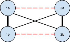
Figure 1: (Color online) An Ising gadget used to convert a given Ising problem into a new Ising problem with twice as many spins whose solution all have zero magnetization. The solutions of the problems in the standard basis are in one-to-one correspondence. This is achieved by appropriately coupling pairs of spins where each pair represents a spin from the original problem. Depicted is the appropriate couplings in the new graph if spins $i$ and $j$ were connected with coupling strength $J$. The pairing coupling is given by $C=4d_{max}J_{max}$ with $d_{max}$ the maximum degree and $J_{max}$ the largest coupling in the given graph.

We will now turn to a set of Hamiltonians where the Hartree-Fock problem is NP-complete even when we restrict ourselves to translationally invariant Slater determinants.

III.1 Gadgets enforcing half filling

We will again like to assume a fixed particle number, more concretely half filling. As the usual embedding of spins into fermions maps the number of electrons to number of ‘up’ spins, we have to build up Ising models where the ground state has zero magnetization. In the present example this will be done by introducing an Ising gadget similar to the pair-orbital construction used to map spin systems to fermionic systems.Schuch and Verstraete (2009); Whitfield, Love, and Aspuru-Guzik (2013) The idea is to fix the zero magnetization by introducing pairs of spins $j\alpha$ and $j\beta$ to represent single spin $j$ in the original Ising spin glass system. Strong anti-ferromagnetic coupling between $j\alpha$ and $j\beta$ enforce anti-parallel alignment. To ensure that the mapped spins are correctly paired, selecting the pair coupling strength, $\mathcal{C}$, to be four times the maximum degree, $d_{max}$, of a spin is sufficient. If $j=+1$, then we should have $(j\alpha,j\beta)=(+1,-1)$ and, if $j=-1$, then $(j\alpha,j\beta)=(-1,+1)$. Coupling, $J_{ij}$, between two spins $i$ and $j$ is effected by letting

$$J_{i\beta,j\beta}=J_{i\alpha,j\alpha}=-J_{i\alpha,j\beta}=-J_{i\beta,j\alpha}=J_{ij}\,.$$

This gadget is depicted in Fig. 1. The energy of the new Hamiltonian, $E^{\prime}$, is

$$E^{\prime}=4E-N\mathcal{C}.$$

III.2 NP-completeness

Now we show that there is an embedding of arbitrary NP-complete Ising problems into instances of the Hartree-Fock method applied to translationally invariant system. In other words, we wish to design a mapping from a given set of couplings $\left\{J_{ij}\in\mathcal{Z}\right\}$ to the sets $\{h_{ij}:h_{ij}=h_{i+1,j+1}\}$ and $\{h_{ijkl}:h_{ijkl}=h_{i+1,j+1,k+1,l+1}\}$ defining a one- and two-body fermionic Hamiltonian with mean-field energy equal to the energy of Ising system $H(\{J_{ij}\})$.

To begin, assume that $\{J_{ij}\}$ has been fixed and the total magnetization is zero. We now consider the case where there are $M$ orbitals and $N=M/2$ fermions in the system. Returning to Eq. (7), we expand the summation over all basis functions and use an indicator vector $R$ where $R_{i}=1$ if orbital $i$ is occupied and zero otherwise. Since the Ising spins take values $\pm 1$, we convert from $R$ to $S$ using $R=(S+1)/2$. Putting this together,

$$P_{pq}=\sum_{i=1}^{M}C_{pi}R_{i}C_{qi}^{*}=\frac{1}{2}\sum_{i=1}^{M}S_{i}C_{pi}C_{qi}^{*}+\frac{1}{2}\delta_{pq}.$$ (20)

We have assumed that the atomic orbital basis is orthogonal and used the fact that $CC^{\dagger}=\mathbf{1}$. Next, we express the Hartree-Fock energy in terms of $S_{i}=\pm 1$ by substituting into Eq. (8):

$$E(P) = -\sum_{ij}\left[\frac{1}{8}\sum_{pqrs}C_{pi}^{*}C_{qi}C_{rj}^{*}C_{sj}A_{prqs}\right]S_{i}S_{j}$$ (21)

$$+\sum_{j}\left[\frac{1}{4}\sum_{pq}C_{qj}C_{pj}^{*}\left(2h_{pq}+\sum_{r}A_{prrq}\right)\right]S_{j}$$

$$+\frac{1}{2}\sum_{p}h_{pp}+\frac{1}{8}\sum_{pr}A_{prrp}\,.$$

To obtain the energy function of $H(\{J_{ij}\})=-\sum_{ij}J_{ij}S_{i}S_{j}$, we would like the single spin Hamiltonian to be zero so we define $h_{pq}:=-\sum_{r}A_{prrq}/2$.

Before enforcing equality for the two-spin interactions, we make use of the translational invariance of the Hamiltonian. If we restrict the trial states to translationally invariant Slater determinants, the fact that $H_{1}$ possesses translation symmetry implies that the mean-field potential is also translation-invariant: $G_{pq}=\sum_{rs}P_{sr}A_{prsq}=\sum_{rs}P_{s+1,r+1}A_{p+1,r+1,s+1,q+1}=G_{p+1,q+1}$. As a result, the eigenvectors of the Fock matrix are given by

$$\left|\hat{k}\right\rangle=\frac{1}{\sqrt{M}}\sum_{x={1}}^{M}e^{-2\pi ikx/M}|x\rangle\,{.}$$ (22)

Thus, $F$ is brought to diagonal form by $C_{kn}=\exp(-i2\pi kn/M)/\sqrt{M}$ as $CFC^{\dagger}=\Lambda$.

Despite knowing the eigendecomposition, selecting the correct orbitals is still NP-hard. We prove this statement by equating $J_{ij}$ from the Ising problem to the two-body interaction of the fermionic system $J_{ij}=\sum_{pqrs}C_{pi}^{*}C_{qi}C_{rj}^{*}C_{sj}A_{prsq}/8$. We utilize the Fourier transform to get the appropriate form and account for the anti-symmetry of the $A$ explicitly,

$$A_{pqrs} = -\frac{8}{M}\sum_{tu}C_{pt}C_{qu}(C_{ru}C_{st}-C_{su}C_{rt})^{*}J_{tu}.$$ (23)

A simple calculation verifies that the inverse Fourier transform of $A_{pqrs}$ with pairs $(m,p-s)$ and $(n,q-r)$ leads to $J_{mn}$ as desired.

After setting $h_{pq}=-\sum_{r}A_{prrq}/2$, we have a fermionic Hamiltonian with Hartree-Fock energy

$$E_{HF}(S)=H_{I}(S)+\sum_{mn}J_{mn}.$$ (24)

This mapping between the two problems requires polynomial time overhead implying that the Hartree-Fock for translationally invariant systems is NP-complete.

III.3 Numerical considerations

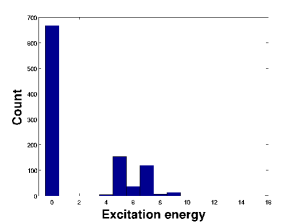
Figure 2: Histogram of excitation energies found using the Hartree-Fock algorithm on 1000 instances derived from the spin glass corresponding to the coupling matrix of Eq. (25).

It is known that the commutator of the charge density and Fock operators is zero, $[P,F]=0$, at local minima including the true Hartree-Fock global minimum. For this reason, the direct inversion iterative subspace method Pulay (1980) utilizes the norm of the $[P,F]$ commutator to accelerate convergence. However, in our model, all the translationally invariant states are local minima and thus the commutator is always zero. While this is no longer a useful error measure, other measures such as the energy based direct inversion iterative scheme Kudin, Scuseria, and Cancès (2002) can still be useful.

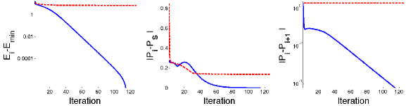
Figure 3: Comparison of successful (solid blue) and unsuccessful (dashed red) self-consistent field method runs. The unsuccessful run converged to $E=-5$ instead of $E=-10$ in the successful run. In the leftmost plot, the convergence to the final energy is shown to be exponential in both cases. The middle plot is the norm of $P-SPS^{\dagger}$ where $S$ is the shift operator. It shows that as the algorithm progresses, the SCF method finds the translationally invariant subspace. Finally, in the last plot, the change in norm between subsequent iterations is plotted. In the non-convergent case, the distance between steps stays approximately two but decays slightly after each iteration.

To illustrate the mapping described, we explore the utility of the Hartree-Fock self-consistent formulation on a test spin glass with coupling matrix

$$J=\left[\begin{array}[]{rrrrrr}0&-1&-1&-1&0&-1\\ &0&1&0&1&1\\ &&0&1&1&0\\ &&&0&\phantom{-}1&1\\ &&&&0&-1\\ &&&&&0\end{array}\right].$$ (25)

The spectrum of the spin Hamiltonian is $\{-10,-6,-2,2,6\}$ and the system has ground states ${s}=[-1,1,1,1,1,1]$ and $-{s}$. After converting this to an instance of Hartree-Fock, we examined 1000 runs of the basic self-consistent algorithm limited to 128 cycles. Beginning from Haar distributed charge density matrices, we found that the algorithm converged on 570 of 1000 instances and an additional 98 instances found the ground state energy despite failing to converge within 128 cycles. A histogram of the results is shown in figure 2. We provide also an example of converged and unconverged instances in figure 3.

IV Conclusion

We continued the line of inquiry of Hamiltonian complexity Osborne (2012) in the context of chemistryWhitfield, Love, and Aspuru-Guzik (2013) with a study of the complexity of the translationally invariant Hartree-Fock problem, proving that it is NP-complete. It is worth pointing out that our results utilize highly spatial non-local Hamiltonians since the models are local in Fourier space. The non-locality is likely to be required in order to allow enough parameters for the models to be both NP-hard and translationally invariant. However, there are some hardness results in this direction for local and translationally invariant systems.Gottesman and Irani (2013)

This work is the first in a series of inquiries aiming to understand the appearance of difficult instances of the Hartree-Fock and post-Hartree-Fock algorithms. With the mappings provided here, we also open the door to using the self-consistent method in the study of spin glasses. The implications of computer science in chemistry has yet to be fully explored; these studies, together with other recent work, are the first steps in this direction.

References

- Hartree (1928) D. Hartree, Proc. Camb. Phil. Soc. 24, 89 (1928).
- Fock (1930) V. Fock, Z. Phys. 61, 723 (1930).
- Goedecker (1999) S. Goedecker, Rev. Mod. Phys. 71, 1085 (1999).
- Pulay (1980) P. Pulay, Chem. Phys. Lett. 73, 393 (1980).
- Saunders and Hillier (1973) V. R. Saunders and I. H. Hillier, Intl. J. Quant. Chem. 7, 699 (1973).
- Bacskay (1981) G. B. Bacskay, Chem. Phys. 61, 385 (1981).
- Veeraraghavan and Mazziotti (2014a) S. Veeraraghavan and D. A. Mazziotti, J. Chem. Phys. 140, 124106 (2014a).
- Veeraraghavan and Mazziotti (2014b) S. Veeraraghavan and D. A. Mazziotti, Phys. Rev. A 89, 010502(R) (2014b).
- Rabuck and Scuseria (1999) A. D. Rabuck and G. E. Scuseria, J. Chem. Phys. 110, 695 (1999).
- Thøgersen et al. (2004) L. Thøgersen, J. Olsen, D. Yeager, P. Jørgensen, P. Salek, and T. Helgaker, J. Chem. Phys. 121, 16 (2004).
- Kudin, Scuseria, and Cancès (2002) K. N. Kudin, G. E. Scuseria, and E. Cancès, J. Chem. Phys. 116, 8255 (2002).
- Schuch and Verstraete (2009) N. Schuch and F. Verstraete, Nature Phys. 5, 732 (2009), also see appendix of arxiv:0712.0483.
- Whitfield, Love, and Aspuru-Guzik (2013) J. D. Whitfield, P. J. Love, and A. Aspuru-Guzik, Phys. Chem. Chem. Phys. 15, 397 (2013).
- Overhauser (1960) A. W. Overhauser, Phys. Rev. Lett. 4, 415 (1960).
- Lykos and Pratt (1963) P. Lykos and G. W. Pratt, Rev. Mod. Phys. 35, 496 (1963).
- Ashcroft and Mermin (1976) N. W. Ashcroft and N. D. Mermin, Solid State Physics (Thomson learning, 1976).
- Stevens (1990) M. P. Stevens, Polymer chemistry (Oxford University Press, New York, 1990).
- Bloch, Dalibard, and Zwerger (2008) I. Bloch, J. Dalibard, and W. Zwerger, Rev. Mod. Phys. 80, 885 (2008).
- Note (1) Let us note here that it is obvious that the Hartree-Fock problems are in NP, as their solution is easy to check.
- Barahona (1982) F. Barahona, J. Phys. A: Math. Gen. 15, 3241 (1982).
- Istrail (2000) S. Istrail, Proc. 32nd ACM Symp. on Theory of Comp. (STOC ’00) , 87 (2000).
- (22) J. D. Whitfield, M. Faccin, and J. D. Biamonte, EPL 99, 57004.
- Lucas (2014) A. Lucas, Front. Physics 2, 5 (2014), 10.3389/fphy.2014.00005.
- Wick (1950) G. C. Wick, Phys. Rev. 80, 268 (1950).
- Shavitt and Bartlett (2009) I. Shavitt and R. J. Bartlett, Many-body methods in chemistry and physics: MBPT and coupled-cluster theory (Cambridge University Press, 2009).
- Osborne (2012) T. J. Osborne, Rep. Prog. Phys. 75, 022001 (2012).
- Gottesman and Irani (2013) D. Gottesman and S. Irani, Theory OF Computing 9, 31 (2013), arXiv:0905.2419.