Abstract

We consider noise-induced transition paths in randomly perturbed dynamical systems on a smooth manifold. The classical Freidlin-Wentzell large deviation theory in Euclidean spaces is generalized and new forms of action functionals are derived in the spaces of functions and the space of curves to accommodate the intrinsic constraints associated with the manifold. Numerical methods are proposed to compute the minimum action paths for the systems with constraints. The examples of conformational transition paths for a single and double rod molecules arising in polymer science are numerically investigated.

1. Introduction

A large number of interesting behaviours of stochastically perturbed dynamical systems are closely related to rare but important transition events between metastable states. Such rare events play a major role in chemical reactions, conformational changes of biomolecules, nucleation events and the like. Theoretical understanding of such transition events and transition paths has attracted a lot of attentions for many years [Kra40, FW98]. The model under consideration is the following (Itô) stochastic differential equations (SDEs) in $\mathbb{R}^{n}$ with small noise amplitude

$$\,\mathrm{d}X_{t}=b(X_{t})\,\mathrm{d}t+\sqrt{\varepsilon}\sigma(X_{t})\,\mathrm{d}W_{t}.$$ (1)

The drift term $b(x)$ could be the gradient form of a potential energy function or have a rather general form. The diffusion matrix $\sigma(x)$ is assumed uniformly non-degenerate. $b$ and $\sigma$ satisfy the regular smoothness conditions that are Lipschitz continuous and bounded.

According to the Freidlin-Wentzell large deviation theory [FW98], in the asymptotics of vanishing noise $\varepsilon\downarrow 0$, the most probable transition pathway is the minimizer of the Freidlin-Wentzell action functional $S$, being

$$S_{T}[\varphi]=\frac{1}{2}\int_{0}^{T}\|{\sigma^{-1}(\varphi)(\dot{\varphi}-b(\varphi)})\|^{2}_{2}\,\mathrm{d}t.$$ (2)

Based on this principle of least action, a few numerical methods, such as the Minimum Action Method (MAM) and its adaptive version [ERVE04, ZRE08], have been proposed and developed for a fixed time interval $[0,T]$ of interest. Another different formulation of the Freidlin-Wentzell theory, based on Maupertuis’ principle [LL76], is the geometric Minimum Action Method (gMAM) on the space of curves [HVE08]. The path given by the gMAM can be viewed as the minimum action path of the original Freidlin-Wentzell action for an optimal $T$. In the special case that $b(x)=-\nabla V(x)$ and $\sigma(x)\equiv 1$, the minimum action path is minimum energy path and the string method [ERVE02] is applicable to identify this path.

In practical applications, the dynamics may be subject to one or more constraints, such as the constant length of rigid molecules, the conservation of mass, etc. These constraints limit the system to live in a particular manifold $\mathcal{M}$, decided by all the constraints, rather than in Euclidean space $\mathbb{R}^{n}$. Even when the stochastic perturbation is applied, the resulting stochastic system still has to satisfy these physical constraints. Thus, one needs to model the stochastic system as an SDE on a manifold $\mathcal{M}$ rather than a deterministic flow $\dot{x}=b(x)$ on $\mathcal{M}$ perturbed by the noise freely in $\mathbb{R}^{n}$. The problem in the latter case is that the perturbed stochastic system does not conserve the quantities associated with $\mathcal{M}$. This subtlety actually implies a different form of the resulting action functional, although in the special case of isotropic noise, i.e., $\sigma(x)\equiv 1$, the action functionals from the two formulations are equivalent. In this reversible case, the modification of the original string method by directly applying the constraints to the path is applicable [DZ09]. It is also justified below in our paper, that the straightforward use of (2) by solving the constraint minimization problem $\inf_{\varphi\in\mathcal{M}}S_{T}[\varphi]$ is applicable when the diffusion tensor $\sigma$ is isotropic.

We present here a rigorous derivation of action functionals for general (non-degenerate) diffusion tensor $\sigma(x)$ by starting from the SDE on the manifold $\mathcal{M}$ with vanishing noise. Although an abstract analogy of Freidlin-Wentzell action functional can be readily accessed (Section 2), the practical application calls for the expressions when the underlying SDE is written on $\mathcal{M}$ as embedded in the Euclidean space $\mathbb{R}^{n}$. This setting up in particular caters for the case under study: $\mathcal{M}=\{x\in\mathbb{R}^{n}:c_{i}(x)=0\}$ where $c_{i}$ are constraints of the system, where a projection operator $\Pi$ from $\mathbb{R}^{n}$ to ${T}\mathcal{M}$, the tangent space of $\mathcal{M}$, can be introduced. By handling the degeneracy issue of the projected diffusion noise, we derive the new forms of action functionals. Our analysis suggests that the resulting forms of action functional on the manifold may differ from the traditional one like Eq. (2). The difference comes from the discrepancy of the metric: The diffusion induces a metric $a(x)=\sigma(x)\sigma(x)^{\textsf{T}}$, and the minimum action path on $\mathcal{M}$ could be viewed as a geodesic (at least for the pure diffusion case when $b=0$) on $\mathcal{M}$ equipped with the metric $a$, but the projection $\Pi$ uses the $L^{2}$-norm of $\mathbb{R}^{n}$.

The paper is organized as follows. We first discuss the stochastic differential equation in the Stratonovich sense on the manifold and the abstract form of the Freidlin-Wentzell action functional on the manifold in Section 2. In Section 3, we consider the manifold embedded in an Euclidean space and introduce the local projection operator to represent the SDE with coordinates formulation. The formula of the action functional are then derived on the space of functions of time and the space of geometric curves. Section 4 is devoted to the numerical methods — the constrained minimum action method. The applications to liquid crystal models are presented in Section 5, where we study the conformational transitions for rod molecules on $\mathbb{S}^{2}$ (unit sphere) and $\mathbb{S}^{2}\times\mathbb{S}^{2}$. In Section 6, we present some outlook for other types of transition paths with constraints beyond our current approach. Finally we make the summary.

2. SDE and large deviation principle on manifolds

The SDE on the manifold is most conveniently written in the Stratonovich sense [Hsu02]. We consider

$$\,\mathrm{d}X_{t}=b(X_{t})\,\mathrm{d}t+\sqrt{\varepsilon}\sum_{k=1}^{L}\sigma_{k}(X_{t})\circ\,\mathrm{d}W_{t}^{k}$$ (3)

on a compact differentiable $d$-dimensional manifold $\mathcal{M}$ without boundary. Here $X\in\mathcal{M}$, the drift and diffusion functions $b,\{\sigma_{k}\}_{k=1}^{L}\in{T}\mathcal{M}$, the tangent bundle of $\mathcal{M}$, and $\{W^{k}\}_{k=1}^{L}$ are independent Wiener processes on $\mathbb{R}$. We assume the non-degeneracy condition for diffusion, i.e.

$$\dim\mbox{span}\{\sigma_{k}(x)\}_{k=1}^{L}=d$$

for any $x\in\mathcal{M}$.

From the large deviation theory on manifolds, under certain regularity conditions on $b$ and $\sigma_{k}$, we have the rate functional (or action functional) $S[\varphi]$ as $\varepsilon$ goes to $0$

$$S_{T}[\phi]=\int_{0}^{T}L(\phi,\dot{\phi})\,\mathrm{d}t,$$ (4)

where $\phi\in C([0,T];\mathcal{M})$ is absolutely continuous, and $\dot{\phi}$ means the derivative with respect to the time $t$. The Lagrangian $L$ is given by the Legendre transformation of the Hamiltonian $H$ as

$$L(x,y)=\sup_{p\in T^{*}\mathcal{M}}\left\{\left\langle p,y\right\rangle-H(x,p)\right\},$$ (5)

where $T^{*}\mathcal{M}$ is the cotangent bundle of $\mathcal{M}$, $y\in T\mathcal{M}$, and $\left\langle\cdot,\cdot\right\rangle$ is the dual product between the spaces $T^{*}\mathcal{M}$ and $T\mathcal{M}$.

For our system (3) the Hamiltonian $H$ has the form

$$H(x,p)=\left\langle p,b(x)\right\rangle+\frac{1}{2}\sum_{k=1}^{L}\left|\left\langle p,\sigma_{k}(x)\right\rangle\right|^{2}.$$

Since $H$ is just a quadratic form of $p$, we have the equation for the critical point of (5)

$$\frac{\partial H}{\partial p}=b(x)+\sum_{k=1}^{L}\left\langle p,\sigma_{k}(x)\right\rangle\sigma_{k}(x)=y.$$ (6)

Note that the type $(0,2)$ covariant symmetric tensor field

$$\sum_{k=1}^{L}\sigma_{k}\otimes\sigma_{k}\in T^{2}_{0}\mathcal{M}$$

can also be viewed as a mapping

$$a:=\sum_{k=1}^{L}\sigma_{k}\otimes\sigma_{k}:T^{*}\mathcal{M}\longrightarrow T\mathcal{M}$$

by fixing its first or second argument [BG80]. From the non-degeneracy condition, we have that the mapping $a$ is bijective, thus its inverse $a^{-1}:T\mathcal{M}\rightarrow T^{*}\mathcal{M}$ is well-defined. Solving the equation (6) we get $p=a^{-1}(y-b(x))$ and thus

$$L(x,y)=\frac{1}{2}\left\langle a^{-1}(y-b(x)),y-b(x)\right\rangle.$$ (7)

To end this section, we comment on the equivalence of the action functionals in the large deviation theory for Stratonovich SDEs and Itô SDE. The equivalent Itô SDEs corresponding to Eq. (3) has an additional term with order $O(\varepsilon)$ besides the original $b$. However, this additional $O(\varepsilon)$ term uniformly vanishes as $\varepsilon\downarrow 0$ if $\sigma$ and its derivative are bounded. Thus, by this fact, as shown in [FW98], this SDE (3) shares the same large deviation result with the one written in the Itô sense.

3. Action Functional

The abstract formulation Eqs. (4) and (7) in Section 2 of the action functional for SDE on the manifold is applicable for many realistic problems. To be more tractable, we consider the manifold $\mathcal{M}$ embedded in the Euclidean space $\mathbb{R}^{n}$, then the SDE on $\mathcal{M}$ can be treated as an SDE in $\mathbb{R}^{n}$ and the standard Freidlin-Wentzell action functional can be explicitly calculated. To represent the aforementioned embedding, we need introduce the projection operator for $\mathcal{M}$.

3.1. Projection and its inverse

Assume that $\mathcal{M}$ is embedded in the Euclidean space $\mathbb{R}^{n}$ ($n\geq d$). We introduce $\Pi_{x}:\mathbb{R}^{n}\rightarrow T_{x}\mathcal{M}\subset\mathbb{R}^{n}$, the orthogonal projection operator at point $x$ on the considered $d$ dimensional manifold $\mathcal{M}$. Given a vector field $b:\mathbb{R}^{n}\rightarrow\mathbb{R}^{n}$ and a uniformly nondegenerated diffusion tensor $\sigma:\mathbb{R}^{n}\rightarrow\mathbb{R}^{n\times m}$ $(m\geq n)$, the process of interest on $\mathcal{M}$ is of the following projection form

$$dX=\Pi\Big{(}b(X)\,\mathrm{d}t+\sqrt{\varepsilon}\sigma(X)\circ\,\mathrm{d}W\Big{)},$$ (8)

where $\Pi=\Pi_{X}$. The subindex of the projection $\Pi$ is sometimes dropped out henceforth. For each sample trajectory in the probability space, if the initial condition $X_{0}=x\in\mathcal{M}$, the solution of Eq. (8) $X_{t}$ is always on the manifold $\mathcal{M}$ for any time $t>0$.

The Hamiltonian for the SDE (8) [FW98, HVE08] is

$$H(x,p)=\left\langle\Pi b(x),p\right\rangle+\frac{1}{2}\left\|{\sigma(x)^{\textsf{T}}}\Pi p\right\|^{2},~{}~{}~{}\forall x,p\in\mathbb{R}^{n},$$

where $\left\langle\cdot,\cdot\right\rangle$ and $\|\cdot\|$ are the inner product and $L^{2}$ norm of $\mathbb{R}^{n}$, respectively. We note that $\Pi^{\textsf{T}}=\Pi$ since it is an orthogonal projection. The corresponding Lagrangian is defined by the Legendre transformation as follows

$$\begin{split}L(x,y)&=\sup_{p\in\mathbb{R}^{n}}\Big{(}\left\langle y,p\right\rangle-H(x,p)\Big{)}\\ &=\sup_{p\in\mathbb{R}^{n}}\left(\left\langle y-\Pi b(x),p\right\rangle-\frac{1}{2}\|{\sigma(x)^{\textsf{T}}}\Pi p\|^{2}\right).\end{split}$$ (9)

For any $x$, $\Pi:\mathbb{R}^{n}\to{T}_{x}\mathcal{M}$ is the projection at this point $x$. Then, each vector $p\in\mathbb{R}^{n}$ can be written as $p=p_{1}+p_{2}$ where $p_{1}$ is in the image space, $\mbox{Img}(\Pi)$ and $p_{2}$ is in the kernel space, $\mbox{Ker}(\Pi)$. Since $p_{1}=\Pi p$ and $\left\langle p_{2},\Pi b\right\rangle=0$, then

$$\begin{split}L(x,y)&=\sup_{p_{1}\in\mbox{Img}(\Pi),p_{2}\in\mbox{Ker}(\Pi)}\left(\left\langle y,p_{2}\right\rangle+\left\langle y-\Pi b(x),p_{1}\right\rangle-\frac{1}{2}\|{\sigma(x)^{\textsf{T}}}p_{1}\|^{2}\right).\end{split}$$

If $y\notin\mbox{Img}(\Pi)$, then the $\left\langle y,p_{2}\right\rangle$ term on the right hands side of the preceding equation can grow infinitely large and in this case, $L=+\infty$. Hence, we only need to consider the case that $y\in\mbox{Img}(\Pi)$ henceforth, then it follows that

$$\begin{split}L(x,y)&=\sup_{p_{1}\in\mbox{Img}(\Pi)}\left(\left\langle y-\Pi b(x),p_{1}\right\rangle-\frac{1}{2}\|{\sigma(x)^{\textsf{T}}}p_{1}\|^{2}_{2}\right).\end{split}$$

To solve the above constrained convex optimization problem, we seek its dual solution. Define the optimization Lagrangian function $\mathcal{L}:\mathbb{R}^{n}\times\mathbb{R}^{n}\to\mathbb{R}$ as

$$\mathcal{L}{(p,\lambda)}=\left\langle y-\Pi b(x),p\right\rangle-\frac{1}{2}\|{\sigma(x)^{\textsf{T}}}p\|^{2}_{2}+\left\langle\lambda,({I}-\Pi)p\right\rangle$$

and the dual function $g(\lambda)=\sup_{p\in\mathbb{R}^{n}}\mathcal{L}(p,\lambda)$ for $\lambda\in\mathbb{R}^{n}$, where $I$ is the identity matrix. The optimal $p$ in definition of $g$ is

$$p^{*}=a^{-1}(y-\Pi b+(I-\Pi)\lambda)$$

where $a^{-1}$ is the inverse of the positive-definite matrix $a(x)=\sigma(x)\sigma(x)^{\textsf{T}}$ evaluated at $x$. So the dual function is

$$g(\lambda)=\mathcal{L}(p^{*},\lambda)=\frac{1}{2}\left\|y-\Pi b(x)+(I-\Pi)\lambda\right\|^{2}_{a}.$$

Here the $a$-weighted norm $\|u\|_{a}$ associated with the positive definite matrix $a(x)$ is $\sqrt{u^{\textsf{T}}a^{-1}u}$ evaluated at $x$. Likewise, the $a$-weighted inner product is defined by $\left\langle u,v\right\rangle_{a}:=u^{\textsf{T}}a^{-1}v$ for $u,v\in\mathbb{R}^{n}$.

It is clear that for the quadratic optimization problem, the strong duality holds. So, we have

$$L(x,y)=\inf_{\lambda}\ g(\lambda)=\inf_{\lambda}\ \frac{1}{2}\left\|y-\Pi b(x)+(I-\Pi)\lambda\right\|^{2}_{a}.$$

By introducing

$$u=y-\Pi b(x)+(I-\Pi)\lambda,$$

the infimum of $g$ becomes

$$\inf_{\lambda}g(\lambda)=\min_{u\in\mathbb{R}^{n},\Pi u=y-\Pi b(x)}\frac{1}{2}\|u\|^{2}_{a}.$$

Therefore for $y\in\mbox{Img}(\Pi)$,

$$L(x,y)=\min_{u\in\mathbb{R}^{n},\Pi u=y-\Pi b(x)}\frac{1}{2}\|u\|_{a}^{2}.$$ (10)

By the duality theory, we also have that

$$\frac{\partial L}{\partial y}=p^{*}=a^{-1}u^{*}$$ (11)

where $u^{*}$ is the solution of the minimization problem (10).

From the constraint $\Pi u=y-\Pi b(x)$ for the minimization problem (10), one may formally view $u$ as an element in the set $\Pi^{-1}(y-\Pi b(x))$ which has the minimal $a$-weighted norm. To ease the presentation, we redefine $\Pi^{-1}$ as follows.

Definition 1.

Let $\Pi$ be an orthogonal projection matrix in $\mathbb{R}^{n}$ and $a$ be a positive definite matrix. For any $v\in\mbox{Img}(\Pi)$, we define $\Pi^{-1}v$ as the vector $u^{*}\in\mathbb{R}^{n}$ such that $u^{*}$ solves $\underset{\Pi u=v}{\min}\|u\|_{a}$.

The above defined $\Pi^{-1}v$ for a given $v\in\mbox{Img}(\Pi)$ is unique since $a$ is not singular. We point out that $\Pi^{-1}$ is not exactly an inverse of $\Pi$ in strict sense because although $\Pi\circ\Pi^{-1}$ is identity restricted on the space $\mbox{Img}(\Pi)$, it is generally invalid that $\Pi^{-1}(\Pi v)=v$. This generalized inverse $\Pi^{-1}:\mbox{Img}(\Pi)\to\mathbb{R}^{n}$ depends on the metric induced by $a$. If $a$ is a scalar matrix, then $\Pi^{-1}$ is identity restricted on $\mbox{Img}(\Pi)$. In the following derivation of the action functional for the SDE (8), $a=\sigma\sigma^{T}$ is implicitly applied in the context where $\Pi^{-1}$ appears. Before our derivation, we first point out some useful properties of $\Pi^{-1}$.

Proposition 2.

For every $w\in\mbox{Ker}(\Pi)$ and $v\in\mbox{Img}(\Pi)$, we have

$$\left\langle\Pi^{-1}v,w\right\rangle_{a}=0.$$

Proof.

Let $u^{*}=\Pi^{-1}v$. Define $u_{\theta}=u^{*}+\theta w$, $\forall\theta\in\mathbb{R}$. Then $\Pi u_{\theta}=\Pi u^{*}=v$ for all $\theta$. So, the function $f(\theta)\triangleq\|u_{\theta}\|^{2}_{a}$ has a minimal value $\|u^{*}\|^{2}_{a}$ at $\theta_{0}=0$. Consequently, $f^{\prime}(\theta_{0})=0$ and $\left\langle u^{*},w\right\rangle=0$ follows. ∎

Proposition 3.

For any vector $v\in\mbox{Img}(\Pi)$, it is true that

$$\|\Pi^{-1}v\|_{a}^{2} =\left\langle v,\Pi^{-1}v\right\rangle_{a},$$

$$\|v\|^{2}_{a} =\|\Pi^{-1}v\|^{2}_{a}+\|{v-\Pi^{-1}v}\|^{2}_{a}.$$

Proof.

The first equality is because $v-\Pi^{-1}v\in\mbox{Ker}(\Pi)$ and Proposition 2. Then it follows that $\|v\|^{2}_{a}=\left\langle v,\Pi^{-1}v\right\rangle+\left\langle v,v-\Pi^{-1}v\right\rangle_{a}=\|\Pi^{-1}v\|^{2}_{a}+\left\langle v,v-\Pi^{-1}v\right\rangle_{a}$. Since $\left\langle\Pi^{-1}v,v-\Pi^{-1}v\right\rangle=0$ due to Proposition 2, then $\|v\|^{2}_{a}=\|\Pi^{-1}v\|^{2}_{a}+\|v-\Pi^{-1}v\|^{2}_{a}$.

∎

Proposition 4.

If $\dim\mbox{Ker}(\Pi)=K$, and $\mbox{Ker}(\Pi)=\operatorname{span}\{\xi_{k}:k=1,\cdots,K\}$, then for any $v\in\mbox{Img}(\Pi)$,

$$\|v\|_{a}^{2}=\|\Pi^{-1}v\|_{a}^{2}+\|\hat{v}\|_{M}^{2},$$

where $M=(M_{ij})=\left\langle\xi_{i},\xi_{j}\right\rangle_{a}$, $i,j=1,2,\ldots,K$ and $\hat{v}=(\hat{v}_{k})=\left\langle v,\xi_{k}\right\rangle_{a}$, $k=1,\ldots,K$.

Proof.

Write $v-\Pi^{-1}v=\sum_{k}\lambda_{k}\xi_{k}$, then these $\lambda_{k}$’s minimize $\|v-\sum_{k}\lambda_{k}\xi_{k}\|^{2}_{a}$. So, $\lambda=(\lambda_{1},\lambda_{2},\ldots,\lambda_{K})^{\textsf{T}}$ satisfy $M\lambda=\hat{v}$. Note that $\|v-\Pi^{-1}v\|_{a}^{2}=\|\sum_{k}\lambda_{k}\xi_{k}\|_{a}^{2}=\lambda^{\textsf{T}}M\lambda=\hat{v}^{\textsf{T}}M^{-1}\hat{v}=\|\hat{v}\|_{M}^{2}$. The conclusion is then immediate from Proposition 3. ∎

3.2. Freidlin-Wentzell action functional on $\mathcal{M}$

Given a starting point $A$ and an ending point $B$ on $\mathcal{M}$ as well as a fixed time interval $[0,T]$, we consider an absolute continuous path $\phi$ on the manifold $\mathcal{M}$ connecting the two points $\phi(0)=A$ and $\phi(T)=B$. By Eqs. (4) and (10), the action functional (or the rate function) for SDE (8) in the vanishing noise limit is

$$S_{T}^{\mathcal{M}}[\phi]=\begin{cases}\underset{u}{\inf}\bigg{\{}\frac{1}{2}\int_{0}^{T}\|u\|_{a}^{2}\,\mathrm{d}t:\ \dot{\phi}-\Pi b(\phi)=\Pi u,\phi(0)=A,\phi(T)=B\bigg{\}},~{}~{}\mbox{ if }\dot{\phi}\in\mbox{Img}\Pi_{\phi}\\ +\infty,~{}~{}~{}\mbox{ otherwise}.\end{cases}$$ (12)

Here the projection $\Pi=\Pi_{\phi(t)}$. Since the admissible path $\phi$ (i.e., $S^{\mathcal{M}}_{T}[\phi]<\infty$) has its tangent $\dot{\phi}$ in the tangent space of the manifold $\mathcal{M}$, the entire admissible path $\phi$ is on $\mathcal{M}$. The form of the functional Eq. (12) can also be formally derived by the contraction principle [Var84, FW98].

In (12), $u$ is a function of $t$ and is equal to $\Pi^{-1}(\dot{\phi}-\Pi b)$ for $t\in[0,T]$ by Definition 1. Then the action functional (12) (for finite value) is

$$S_{T}^{\mathcal{M}}[\phi]=\frac{1}{2}\int_{0}^{T}\left\|\Pi^{-1}(\dot{\phi}-\Pi b)\right\|_{a}^{2}\,\mathrm{d}t$$ (13)

defined over the admissible set

$$\begin{split}\mathcal{A}=\{\phi\in C([0,T];\mathcal{M}):\phi(0)=A,\phi(T)=B,~{}\phi\mbox{ is absolutely continuous}\},\end{split}$$ (14)

which is equivalent to

$$\begin{split}\mathcal{A}^{\prime}=\{\phi\in C([0,T];\mathbb{R}^{n}):&~{}~{}\dot{\phi}\in\mbox{Img}\Pi_{\phi},\phi(0)=A,\phi(T)=B,\\ &~{}~{}\phi\mbox{ is absolutely continuous}\}.\end{split}$$ (15)

When the noise is isotropic, i.e., $\sigma(x)$ is a scalar matrix $\sigma I$, then $\|u\|_{a}=\|u\|/\sigma^{2}$. In such a case, $\Pi^{-1}$ is identity. Then the principle of least action is

$$\inf_{\phi\in\mathcal{A}}S^{1}_{T}[\phi]$$

where

$$S^{1}_{T}[\phi]\triangleq\frac{1}{2}\int_{0}^{T}\left\|\dot{\phi}-\Pi b(\phi)\right\|_{a}^{2}\,\mathrm{d}t.$$ (16)

This $S^{1}_{T}$ is the action functional corresponding to an SDE similar to Eq. (8), but without the projection of the random forcing term, i.e.,

$$\,\mathrm{d}X=\left(\Pi b(X)\right)\,\mathrm{d}t+\sqrt{\varepsilon}\sigma(X)\,\mathrm{d}W,$$

whose solution $X_{t}$ is not on $\mathcal{M}$. In general, these two actions are different and satisfy

$$S^{\mathcal{M}}_{T}[\phi]\leq S^{1}_{T}[\phi]$$

by Proposition 4.

Remark 5.

One naive approach might be to solve the following minimization problem

$$S^{0}[\phi]=\bigg{\{}\frac{1}{2}\int_{0}^{T}\|\dot{\phi}-b(\phi)\|_{a}^{2}\,\mathrm{d}t:\Pi\dot{\phi}=\dot{\phi},\ \phi(0)=A,\phi(T)=B\bigg{\}}.$$ (17)

Note that $S^{0}-S^{1}=\frac{1}{2}\int_{0}^{T}\|b(\phi)-\Pi b(\phi)\|_{a}^{2}dt$. Even for the gradient system and isotropic constant diffusion $a=\sigma^{2}I$, the solutions for $S^{0}$ and $S^{1}$ are different. It is not correct to use $S^{0}$ for the constrained SDE problem.

If we furthermore assume that $b(x)=-\nabla V(x)$ and $\sigma(x)={I}$, then the system is a gradient system on $\mathcal{M}$. The variational problem $\inf_{T}\inf_{\phi\in\mathcal{A}}S^{1}_{T}[\phi]$ has a solution which is the minimum energy path on $\mathcal{M}$ which satisfies that $\dot{\phi}\parallelslant\Pi b(\phi)$ and it follows that the extension of the string method works for this case by evolving each image on the string according to the flow $\Pi b(x)$ on $\mathcal{M}$ and applying the reparametrization on $\mathcal{M}$. So, our above derivation justifies the algorithm [DZ09] for this gradient case, but our form (13) is applicable to general cases.

3.3. Geometric action functional on $\mathcal{M}$

The geometric formulation of the action function, developed in [HVE08], does not involve time explicitly and allow the variation of the time interval. If we consider the original formulation of Freidlin-Wentzell theory as analogy of Lagrangian mechanics for the trajectory of a particle, then the geometric action functional in [HVE08] correspond to the Maupertuis’ principle ($\S 44$, [LL76]) for the curve the particle travels.

In the next, we consider the geometric action functional $\hat{S}$ for the SDE (8) on the manifold $\mathcal{M}$. Suppose that a curve $\gamma$ on $\mathcal{M}$ is parametrized as $\gamma=\varphi(\alpha)$, with $\alpha\in[0,1]$, for instance, $\alpha$ being the arc length parameter. Then the geometric action (also called abbreviated action [LL76]) is the following line integration along $\gamma$

$$\hat{S}[\varphi]=\int_{\gamma}\left\langle p,\,\mathrm{d}\varphi\right\rangle$$

subject to the constraint $H(\varphi,p)=0$, where $p=\partial L/\partial y(\varphi,\dot{\varphi})$ is the generalized momentum, $L$ is the Lagrangian defined in (9) and $\dot{\varphi}$ is the time derivative (velocity). By Eq. (11), this generalized momentum is

$$p=a^{-1}\Pi^{-1}(\dot{\varphi}-\Pi b(\varphi)).$$ (18)

So, $\hat{S}$ has the following expression,

$$\begin{split}\hat{S}[\varphi]&=\int\left\langle a^{-1}\Pi^{-1}(\dot{\varphi}-\Pi b(\varphi)),\,\mathrm{d}\varphi\right\rangle\\ &=\int_{0}^{1}\left\langle\Pi^{-1}({\varphi}^{\prime}\lambda-\Pi b(\varphi)),\varphi^{\prime}\right\rangle_{a}\,\mathrm{d}\alpha\end{split}$$

where the scalar-valued function $\lambda:=\,\mathrm{d}\alpha/\,\mathrm{d}t\in[0,+\infty]$ is the change of variable between the physical time $t$ and the arc length $\alpha$. Here $\dot{\varphi}=d\varphi/\,\mathrm{d}t$ is the time derivative and ${\varphi}^{\prime}=d\varphi(\alpha)/d\alpha$ is the tangent vector of the curve for the $\alpha$-parametrization. To derive the expression of $\lambda$ in terms of $\varphi$ and $\varphi^{\prime}$, we use the condition that the Hamilton along the trajectory is the constant zero [HVE08, LL76]. Plugging in the generalized momentum given in Eq. (18), we solve $\lambda$ from the following zero-valued Hamiltonian,

$$H(\varphi,p)=\left\langle\Pi b(\varphi),\Pi^{-1}(\dot{\varphi}-\Pi b(\varphi))\right\rangle_{a}+\frac{1}{2}\left\|\Pi^{-1}(\dot{\varphi}-\Pi b(\varphi))\right\|_{a}^{2}=0.$$

Since $\dot{\varphi}=\varphi^{\prime}\lambda$, the above equation gives the result that

$$\begin{split}\frac{1}{2}\lambda^{2}\|\Pi^{-1}\varphi^{\prime}\|_{a}^{2}+\lambda\left\langle\Pi b(\varphi)-\Pi^{-1}\Pi b(\varphi),\Pi^{-1}\varphi^{\prime}\right\rangle_{a}\\ +\frac{1}{2}\left\|\Pi^{-1}\Pi b(\varphi)\right\|_{a}^{2}-\left\langle\Pi b(\varphi),\Pi^{-1}\Pi b(\varphi)\right\rangle_{a}=0.\end{split}$$

By the Proposition 2 and Proposition 3 , it is further simplified as

$$\frac{1}{2}\lambda^{2}\|\Pi^{-1}\varphi^{\prime}\|_{a}^{2}-\frac{1}{2}\|\Pi^{-1}\Pi b(\varphi)\|_{a}^{2}=0.$$

Since $\lambda>0$, we choose the positive root of the above quadratic equation,

$$\lambda=\frac{\|B\|_{a}}{\|{\nu}\|_{a}}$$ (19)

where

$$B:=\Pi^{-1}\Pi b(\varphi),\qquad\nu:=\Pi^{-1}\varphi^{\prime}.$$

Therefore, we obtain the expression of $\hat{S}$ for $\varphi\in\mathcal{A}$,

$$\begin{split}\hat{S}[\varphi]&=\int_{0}^{1}\left\langle\lambda\Pi^{-1}{\varphi}^{\prime}-\Pi^{-1}\Pi b(\varphi),\varphi^{\prime}\right\rangle_{a}\,\mathrm{d}\alpha\\ &=\int_{0}^{1}\left\langle\lambda\nu-B,\varphi^{\prime}\right\rangle_{a}\,\mathrm{d}\alpha\\ &=\int_{0}^{1}\left\langle\frac{\|B\|_{a}}{\|{\nu}\|_{a}}\nu-B,\varphi^{\prime}\right\rangle_{a}\,\mathrm{d}\alpha\\ &=\int_{0}^{1}{\|B\|_{a}}{\|{\Pi^{-1}\varphi^{\prime}}\|_{a}}-\left\langle B,\varphi^{\prime}\right\rangle_{a}\,\mathrm{d}\alpha.\end{split}$$ (20)

Here, Proposition 2 is used again for the last equality.

4. Constrained Minimum Action Method

So far we have derived two action functionals on $\mathcal{M}$, Eq. (13) on the space of absolution continuous functions $C([0,T],\mathcal{M})$ and Eq. (20) on the space of curves living on $\mathcal{M}$. The variational solutions of these acton functionals will give the minimum action path. The variational problems are solved by numerical optimization solver. We next discuss about the numerical issue of this variational problem for $\mathcal{M}$ being explicitly specified by constraint functions.

Let’s recall that the constraints for the system are specified by non degenerated constraint functions $c_{k}(x)=0$, $k=1,2,\ldots,n-d$. Thus

$$\mathcal{M}=\{x\in\mathbb{R}^{n}:c_{k}(x)=0,k=1,2,\ldots,n-d\}.$$ (21)

The basis vector for the space $\mbox{Ker}(\Pi_{x})$ is $\xi_{k}=\nabla c_{k}(x)$. Explicit formula of $\Pi^{-1}$ can be expressed in terms of $\xi_{k}=\nabla c_{k}$ , following the same procedure as in Proposition 4. Then the variational problem for Eq. (13) and Eq. (20) can be numerically solved under the constraint $\{c_{k}=0\}$ by any modern optimization solver. When the local coordinate representations for Eq. (13) and Eq. (20) are available for some practical problems, the optimization procedure can be performed directly in the local coordinate form.

The calculation of the minimum action curve for the geometric action functional involves a reparametrization step which is based on the calculation of the arc length of the curve $\varphi(\alpha)$. It may be more natural to use the geodesic distance on $\mathcal{M}$ to define the arc length, but it is practically convenient to just use the Euclidean arc length. If the number of discrete images in representing the curve is sufficiently large, these two choices of the distance between neighbouring images measured by geodesic or Euclidean metrics would not give much difference.

In the following, we describe one example of the action functionals for the spherical case $\mathcal{M}=\mathbb{S}^{d}$ where $d=n-1$. When $n=3$, this correspond to the first example in next section of a rigid rod model for liquid crystal. The constraint function for $S^{d-1}$ is $c(x)=\|x\|^{2}-1=0$. The projection onto the tangent space is $\Pi_{x}=I-\boldsymbol{n}(x)\otimes\boldsymbol{n}(x)$ where $\boldsymbol{n}(x)=x/\|x\|$ is the unit ($L^{2}$ norm) normal. $\mbox{Ker}(\Pi_{x})=\{\boldsymbol{n}(x)\}$ and $\mbox{Img}(\Pi_{x})=T_{x}\mathbb{S}^{n-1}$. The calculation in Proposition 4 shows that for any $v\in\mbox{Img}(\Pi)$

$$\Pi^{-1}v=v-\frac{\left\langle v,\boldsymbol{n}\right\rangle_{a}}{\left\langle\boldsymbol{n},\boldsymbol{n}\right\rangle_{a}}\boldsymbol{n}=v-{\left\langle v,\boldsymbol{n}_{a}\right\rangle_{a}}\boldsymbol{n}_{a}$$

and $\|\Pi^{-1}v\|_{a}^{2}=\|v\|_{a}^{2}-{(\left\langle\boldsymbol{n}_{a},v\right\rangle_{a})^{2}}$, where $\boldsymbol{n}_{a}=\boldsymbol{n}/\|\boldsymbol{n}\|_{a}$ is the unit vector in sense of $\|\cdot\|_{a}$ norm. Then, the action functional $S^{\mathcal{M}}_{T}$ in Eq. (12) becomes

$$\begin{split}S^{\mathcal{M}}_{T}[\phi]=&\frac{1}{2}\int_{0}^{T}\left\|\dot{\phi}-\Pi b(\phi)\right\|_{a}^{2}-\left\langle\frac{\phi}{\|\phi\|_{a}},\dot{\phi}-\Pi b(\phi)\right\rangle_{a}^{2}\,\mathrm{d}t.\end{split}$$ (22)

Note that the first term is exactly $S^{1}_{T}$ Eq. (16), and $S^{\mathcal{M}}_{T}[\phi]\leq S^{1}_{T}[\phi]$. Likewise, we have the expression of the geometric action function Eq. (20) in this case, which is

$$\begin{split}\hat{S}[\varphi]=\int_{0}^{1}&\sqrt{\left(\|\Pi b\|^{2}_{a}-\left\langle\Pi b,\varphi\right\rangle^{2}_{a}/\|\varphi\|^{2}_{a}\right)\left(\|\varphi^{\prime}\|^{2}_{a}-\left\langle\varphi^{\prime},\varphi\right\rangle^{2}/\|\varphi\|^{2}_{a}\right)}\\ &-\left\langle\Pi b,\varphi^{\prime}\right\rangle_{a}+\left\langle\Pi b,\varphi\right\rangle_{a}\left\langle\varphi^{\prime},\varphi\right\rangle_{a}/\|\varphi\|^{2}_{a}~{}\mbox{d}\alpha.\end{split}$$

5. Examples

In this section, we apply the constrained minimum action method to study the transition pathways for the motion of one class of liquid crystal molecules. This type of macromolecules are usually modelled as rigid rods so the configuration space for each rod is $\mathbb{S}^{2}$. More realistic models such as general bead-rod-spring models have more complex intrinsic constraints for the molecular configurations; the details are well explained in Chapter 5 of reference [Ött96]. The rigid rod model we are studying here is the typical building block for those chain models.

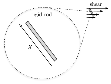
Figure 1. Rigid rod polymeric model in shear flow. The length of the directed vector $\boldsymbol{X}$ is one.

Typically, there are many equilibrium states for the molecular configurations. Depending on the interaction between molecules, there could be some spontaneously preferred directions $\boldsymbol{X}$ for the molecules. In many cases where the ensemble statistics is of interest, the direction $\boldsymbol{X}$ and $-\boldsymbol{X}$ is undistinguished due to symmetry. But at microscopical level, each individual configuration does switch between the symmetric two metastable states $\boldsymbol{X}$ and $-\boldsymbol{X}$. When these macromolecular polymers are added into solvent (Figure 1), then the mixed solution has interesting hydrodynamical and rheological features different from the Newtonian fluid. The study of complex fluid mainly focuses on macroscopic quantities of polymeric fluid, such as viscoelasticity. However, the change of macromolecular configurations at the microscopic level due to thermal fluctuation and fluid shear is of its own interests, in particular when these macromolecules, for instance liquid crystals, are directly responsible for some physical mechanisms in practice such as colour control for display devices.

In the following, we present two examples to understand the transition paths in the rigid rod model. In the first example, we study the single rod molecule with quadratic potential in shear flow. Due to spheric symmetry, any linearly stable state $\boldsymbol{X}$ has a symmetric stable one $-\boldsymbol{X}$. The transition from $\boldsymbol{X}$ to $-\boldsymbol{X}$ corresponds to the flip over process of the rod molecule. How the shear rate impacts this flip over process is of our interest. Our second example includes two rods with interaction between them. This is the simplest case for the weakly interaction particle system [LZZ04]. To see how the anisotropic diffusion tensor play roles in transition path, we artificially assign two different diffusion coefficients, $\sigma_{1}$ and $\sigma_{2}$, for the two rods and investigate the effect of the ratio $\sigma_{2}/\sigma_{1}$ on the transition pathways. Although the diffusion coefficient (i.e., temperature) of two molecules seem to be the same in physical reality, our manipulation of anisotropic noise in this model produces some interesting results, which could be instructive in the general case of the state-dependent noise $\sigma(x)$ and may be quite useful when the precise control of noise size for each individual rod (or two groups of rods) is possible.

Lastly, we remark that we only report the results from the constrained minimum action method based on the geometric action formulation. Thus, the objects we calculated are curves in the phase space. The pathways from the constrained Freidlin-Wentzell action functional are consistent with these results when the underlying time interval is sufficient large.

5.1. Flip over process of one rigid rod

Consider a unit sphere $\mathbb{S}^{2}$ in $\mathbb{R}^{3}$. $X=(X_{1},X_{2},X_{3})\in\mathbb{R}^{3}$. Let $V:\mathbb{R}^{3}\to\mathbb{R}$ be the potential energy with symmetry $V(x)=V(-x)$ and $W_{t}$ be a Brownian motion in $\mathbb{R}^{3}$. Write the normal vector $\boldsymbol{n}(x)=x/\|x\|\in\mathbb{S}^{2}$. The motion of the rod molecule in consideration is described by the following equation,

$$\,\mathrm{d}X=(I-\boldsymbol{n}(X)\boldsymbol{n}(X)^{\textsf{T}})\bigg{(}(-\nabla V(X)+K_{0}X)\,\mathrm{d}t+\sqrt{\varepsilon}\circ\,\mathrm{d}W_{t}\bigg{)}$$

where $K_{0}$ is the matrix of the shear rate tensor in the Cartesian coordinate.

Here the noise is isotropic and the manifold $\mathcal{M}$ is $\mathbb{S}^{2}$. The geometric action functional in Eq. (20) is reduced to

$$\begin{split}\hat{S}[\varphi]&=\int_{0}^{1}{\|\Pi^{-1}\Pi b(\varphi)\|}{\|{\Pi^{-1}\varphi^{\prime}}\|}-\left\langle\Pi^{-1}\Pi b(\varphi),\varphi^{\prime}\right\rangle d\alpha\\ &=\int_{0}^{1}{\|\Pi b(\varphi)\|}{\|{\varphi^{\prime}}\|}-\left\langle\Pi b(\varphi),\varphi^{\prime}\right\rangle d\alpha\end{split}$$ (23)

where ${\|\varphi(\alpha)\|=1}$ for all $\alpha$.

We assume the following quadratic form of the external potential function $V$

$$V(x)=\sum_{i=1}^{3}\frac{1}{2}\mu_{i}x_{i}^{2},\mbox{ where }\mu_{3}>\mu_{2}>\mu_{1}>0.$$ (24)

The two local minima of $V$ on $\mathbb{S}^{2}$ are $\boldsymbol{e}^{(1)}=(1,0,0)$ and $-\boldsymbol{e}^{(1)}=(-1,0,0)$; the two local maxima are $\boldsymbol{e}^{(3)}=(0,0,1)$ and $-\boldsymbol{e}^{(3)}=(0,0,-1)$; the saddles are $\boldsymbol{e}^{(2)}=(0,1,0)$ and $-\boldsymbol{e}^{(2)}=(0,-1,0)$. In the example below, we simply set $(\mu_{1},\mu_{2},\mu_{3})=(1,2,3)$.

For the quadratic potential Eq. (24), the SDE then becomes the following form

$$\,\mathrm{d}X=(I-n(X)n(X)^{\textsf{T}})(KX\,\mathrm{d}t+\sqrt{\varepsilon}\circ\,\mathrm{d}W_{t})$$ (25)

where $K=\mbox{diag}\{\mu_{1},\mu_{2},\mu_{3}\}+K_{0}$. We consider two forms of shear rate matrix $K_{0}$ corresponding to different directions of the shear flow.

5.1.1. Shear flow: example 1

We first consider the following shear flow where $x_{1}$ is the streamwise direction, $x_{2}$ is the shearwise direction and $x_{3}$ is the spanwise direction. So it is assumed that

$$K_{0}=\begin{bmatrix}0&\dot{\gamma}_{12}&0\\ 0&0&0\\ 0&0&0\end{bmatrix}.$$ (26)

Here the shear rate $\dot{\gamma}_{12}$ is a constant parameter.

The deterministic drift flow on $\mathbb{S}^{2}$ is $\dot{X}=(I-\boldsymbol{n}\boldsymbol{n}^{\textsf{T}})KX$. The fixed points of this flow are the following three vectors on $\mathbb{S}^{2}$

$$\boldsymbol{n}^{(1)} = (1,0,0)^{\textsf{T}},$$

$$\boldsymbol{n}^{(2)} = (-\dot{\gamma}_{12},\mu_{2}-\mu_{1},0)^{\textsf{T}}/\sqrt{\dot{\gamma}_{12}^{2}+(\mu_{2}-\mu_{1})^{2}},$$ (27)

$$\boldsymbol{n}^{(3)} = (0,0,1)^{\textsf{T}},$$

and their symmetric counterparts $-\boldsymbol{n}^{(i)},\,i=1,2,3$. In total, there are three pairs of fixed points. Since $\mu_{3}>\mu_{2}>\mu_{1}>0$ in the quadratic potential (Eq. (24)), we can derive the following linear stability results for infinitesimal perturbations. The pair $\pm\boldsymbol{n}^{(1)}$ is linearly stable ( classified as sink and denoted as $si_{+}$ and $si_{-}$, respectively) with two unstable eigen directions $\boldsymbol{e}^{(2)}$ and $\boldsymbol{e}^{(3)}$. The pair of $\pm\boldsymbol{n}^{(3)}$ is linearly unstable (classified as source and denoted as $so_{+}$ and $so_{-}$, respectively). The pair of $\pm\boldsymbol{n}^{(2)}$ is saddle point (and denoted as $sa_{+}$ and $sa_{-}$, respectively) with one stable eigen direction $\boldsymbol{e}^{(3)}$ (the unstable eigen direction relies on $\dot{\gamma}_{12}$). The separatrix on the unit sphere between the two sources $si_{+}$ and $si_{-}$ is the great circle of $\mathbb{S}^{2}$in the plane spanned by $sa_{\pm}$ and $so_{\pm}$.

The introduction of the shear rate in form of Eq. (26) only affects the orientation of the saddle point (Eq. (27)). The positive value of shear rate $\dot{\gamma}_{12}$ has the effect of rotating the saddle direction $\boldsymbol{n}^{(2)}$ counterclockwise (looking down from $x_{3}$-direction, i.e., vertical direction). The negative $\dot{\gamma}_{12}$ gives the opposite rotation direction.

We are concerned with the flip over process of the rigid rod, i.e., the transition between two symmetric stable fixed points $si_{+}=\boldsymbol{n}^{(1)}$ and $si_{-}=-\boldsymbol{n}^{(1)}$. The minimal action for this transition is related to the frequency of this process ( $\propto\exp(-\inf S/\varepsilon)$ [FW98]). The smaller the minimal action, the more frequently the rod flips between two stable states.

To resolve all possible minimizers of the variational problem $\inf_{\varphi\in\mathbb{S}^{2}}\hat{S}[\varphi]$, the initial guesses of the path should be carefully constructed. The idea of setting initial guess is as follows. Since on the separatrix between $si_{+}$ and $si_{-}$, there are four fixed points, $so_{\pm}$ and $sa_{\pm}$. We then construct the different initial paths passing through these points, respectively. In consideration of the symmetry for the case of $so_{\pm}$, we only need to test three different initial guesses, which give three different local minima of the action functional $\hat{S}$. As a result, the obtained three minima correspond to the minimal actions from $si_{+}$ to saddles $sa_{-}$, $sa_{+}$, and $so_{-}$ (or $so_{+}$), respectively. The minimum among these three minimized actions gives the global optimum and thus corresponds to the correct transition path between $si_{-}$ and $si_{+}$. Refer to Figure 2 for the plot of these three actions when the shear rate is varied. This evidence shows that the shear of the flow field lowers the global minimum of the action, hence increase the flip over frequency. At a high shear rate, the frequency could be so large that the rod molecule would oscillate between the direction $si_{-}=-\boldsymbol{n}^{(1)}$ and $s_{+}=\boldsymbol{n}^{(1)}$.

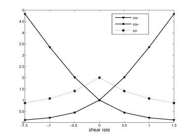
Figure 2. The minimum actions (vertical axis) for three paths from $si_{+}$ to $sa_{-}$, $sa_{+}$ and $so_{\pm}$, respectively.

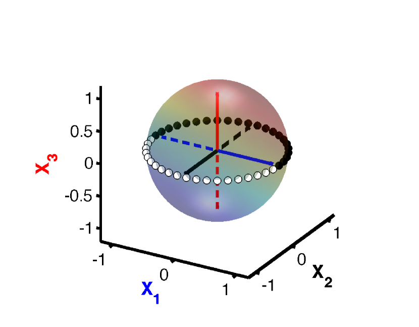
(a) shear rate $\dot{\gamma}_{12}=0$.

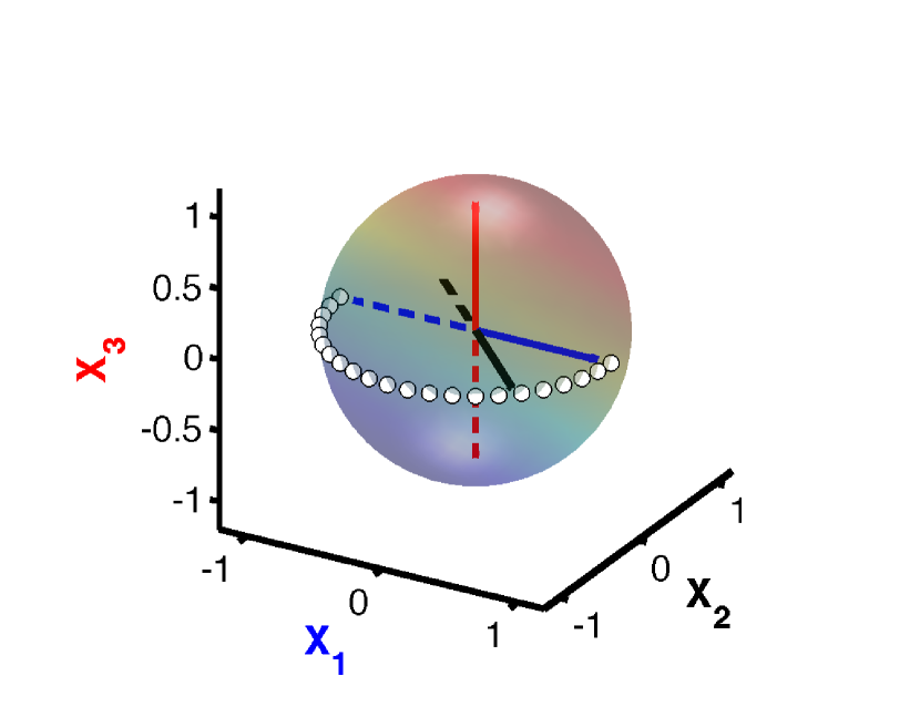
(b) shear rate $\dot{\gamma}_{12}=1.0$

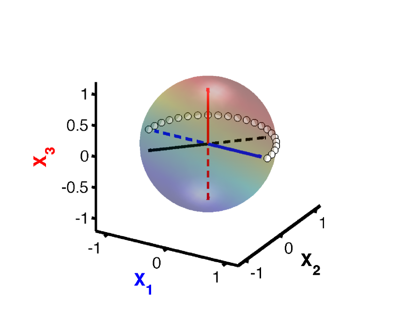
(c) shear rate $\dot{\gamma}_{12}=-1.0$

Figure 3. Global minimum action paths for different shear rates. The two symmetric filp-over paths passing $sa_{-}$ are shown in white and black, respectively.

Among the obtained three paths from different initial guesses, the global minimum is the one passing the saddle $sa_{-}$ or $sa_{+}$, depending on the direction of the shear, i.e., the sign of $\dot{\gamma}_{12}$. These paths are one of semi great circles entirely in the $x_{1}$-$x_{2}$ plane. Figure 3 shows the global minimum action path starting from $si_{+}$ for $\dot{\gamma}_{12}=0,1,-1$. For instance, when $\dot{\gamma}_{12}>0$, the saddle $sa_{-}$ (the solid black line) is shifted closer to $si_{+}$ so that it takes less action for the system to escape from $si_{-}$ to the separatrix by selecting this saddle $sa_{-}$. A similar picture holds for negative $\dot{\gamma}_{12}$ where the saddle $sa_{+}$ (the dashed black line) is shifted closer to $si_{+}$.

5.1.2. Shear flow: example 2

Next we study the transitions with the following shear rate tensor

$$K_{0}=\left[\begin{array}[]{ccc}0&0&\dot{\gamma}_{13}\\ 0&0&0\\ 0&0&0\end{array}\right].$$

The fixed points for this $K_{0}$ become

$$\boldsymbol{n}^{(1)} = (1,0,0)^{\textsf{T}},$$

$$\boldsymbol{n}^{(2)} = (0,1,0)^{\textsf{T}},$$

$$\boldsymbol{n}^{(3)} = (-\dot{\gamma}_{13},0,\mu_{3}-\mu_{1})^{\textsf{T}}/\sqrt{\dot{\gamma}_{13}^{2}+(\mu_{3}-\mu_{1})^{2}}.$$

and $si_{-}=-\boldsymbol{n}^{(1)}$ and $si_{+}=\boldsymbol{n}^{(1)}$ are sinks, $sa_{-}=-\boldsymbol{n}^{(2)}$ and $sa_{+}=\boldsymbol{n}^{(2)}$ are saddles, $so_{-}=-\boldsymbol{n}^{(3)}$ and $so_{+}=\boldsymbol{n}^{(3)}$ are sources. The heteroclinic orbits among these fixed points are similar to the previous example in §5.1.1: They are the great circles connecting the neighbouring fixed points. The separatrix between $si_{+}$ and $si_{-}$ is also the great circle in the plane of $sa$ and $so$. The difference from the example in §5.1.1 is that now the shear rate affects the location of the sources $so_{\pm}$ while the saddles $sa_{\pm}$ are unchanged.

Again, we are interested in the transition from $si_{+}$ to $si_{-}$ and shall examine the minimum action paths with different initial guesses which pass through the fixed points $so_{-}$, $so_{+}$ and $sa_{\pm}$, respectively. Figure 4 shows the minimum actions for these three paths. From this figure, we can observe that a larger shear rate deceases the actions both to the saddle and to the source. However, there is a competition between these two local minima of the action. When the shear rate is small, the path passing the saddle is the global solution. But when the shear rate is very large, the calculation shows that the action to the source can be slightly smaller than the one to the saddle so that the transition state changes from the saddle to the source. This suggests that there is a bifurcation point of the parameter $\dot{\gamma}_{13}^{*}$ (around $1.9$ for this example in our calculation) for the patterns of the global minimum action path.

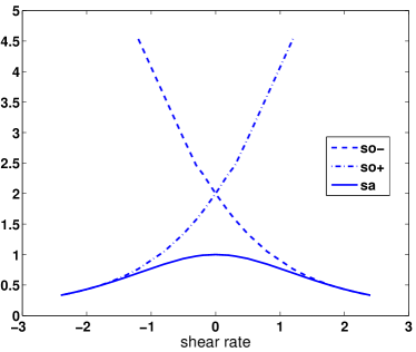
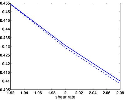
Figure 4. The minimum actions for three paths from $si_{+}$ to $so_{-}$, $so_{+}$ and $sa_{\pm}$ (either $sa_{-}$ or $sa_{+}$ since the minimal actions are the same due to symmetry), respectively. When $\dot{\gamma}_{13}$ passes the critical value $\dot{\gamma}^{*}_{13}\approx 1.9$, the global minimum path changes from passing o $sa$ to passing $so_{-}$, i.e., the transition state changes from $sa$ to $so_{-}$. The right panel is the zoom of the left panel for a window near $\dot{\gamma}_{13}=2$.

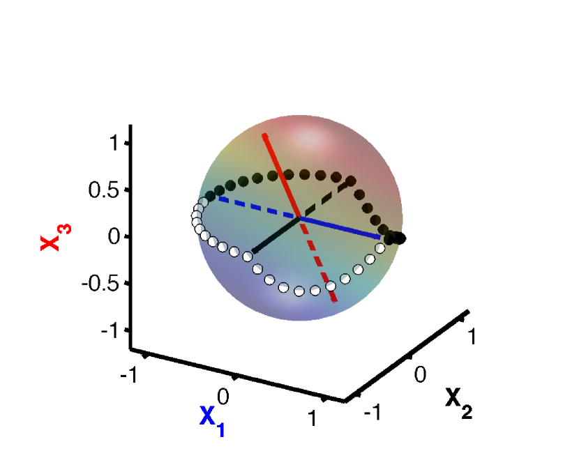
(a) shear rate $\dot{\gamma}_{13}=1.0.$

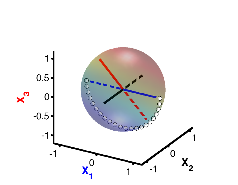
(b) shear rate $\dot{\gamma}_{13}=2.0$

Figure 5. Global minimum action paths for different shear rates. (a): The transition path from $si_{+}$ to $si_{-}$ through $sa_{-}$ and its symmetric mirror are both shown. (b) The path is the semi-circle in the plan spanned by $so$ and $si$ ($x_{1}$-$x_{3}$ plane) . The initial guess of the path in the minimum action method is the path in Figure 5(a).

The above conclusion can be better understood if we plot the global minimum action path for $\dot{\gamma}_{13}=1$ and $2$ in Figure 5. The positive value of shear rate $\dot{\gamma}_{13}$ has the effect of tilting the unstable fixed point $so_{+}=\boldsymbol{n}^{(3)}$ (the solid red line) counter-clockwisely in the $x_{1}$-$x_{3}$ plane (looking from $-x_{2}$-direction). Such tilts will pull $so_{-}$ (the dashed red line) towards $si_{+}$ (the solid blue line) and push $so_{+}$ away from $si_{+}$. However, when the shear rate is not strong, this push is not significant enough to beat the action of the path through the saddle $sa_{\pm}$ (the pair of curves shown in Figure 5(a) ). When $\dot{\gamma}_{13}$ continues to increase by passing the critical value $\dot{\gamma}^{*}_{13}$, the shear-induced tilt will become strong enough to lower the action to reach $so_{-}$ significantly so as to become a global soluiton.

In summary, when the shear of the fluid affects the unstable fixed points $so_{\pm}$ of the molecular configuration on $\mathbb{S}^{2}$, the competition of the minimum action paths passing through the saddle $sa_{\pm}$ or through the source $so_{\pm}$ would generate a bifurcation of the patterns of the global path. The same phenomena have been observed before, for instance, in some planer (non-gradient) system [MS93]. For real problems, the shear rate tensor $K_{0}$ may be the combination of the above two examples we have studied; from the analysis above, we expect that the similar bifurcation of the pathways could happen for different size of the shear rate. It is also generally believed that the shear would lower the global minimum action, thus increase the flip over frequency.

5.2. Flip over of two rigid rods

Here, we study a slight generalization of the previous studied single rod case, a toy model of two interactive rigid rods. Let $\boldsymbol{X}_{1},\boldsymbol{X}_{2}$ be the directed unit vector of two rods. We consider the following stochastic dynamics on $\mathbb{S}^{2}\times\mathbb{S}^{2}$,

$$\left\{\begin{aligned} \,\mathrm{d}\boldsymbol{X}_{1}&=(I-\boldsymbol{n}_{1}\boldsymbol{n}_{1}^{\rm T})(-\nabla V(\boldsymbol{X}_{1})\,\mathrm{d}t-\nabla_{\boldsymbol{x}_{1}}U(\boldsymbol{X}_{1},\boldsymbol{X}_{2})\,\mathrm{d}t+\sigma_{1}\sqrt{\epsilon}\circ\,\mathrm{d}\boldsymbol{W}_{1}),\\ \,\mathrm{d}\boldsymbol{X}_{2}&=(I-\boldsymbol{n}_{2}\boldsymbol{n}_{2}^{\rm T})(-\nabla V(\boldsymbol{X}_{2})\,\mathrm{d}t-\nabla_{\boldsymbol{x}_{2}}U(\boldsymbol{X}_{1},\boldsymbol{X}_{2})\,\mathrm{d}t+\sigma_{2}\sqrt{\epsilon}\circ\,\mathrm{d}\boldsymbol{W}_{2}),\end{aligned}\right.$$ (28)

where $\boldsymbol{n}_{i}=\boldsymbol{X}_{i}/\|\boldsymbol{X}_{i}\|,\,i=1,2$. $\sigma_{1}$ and $\sigma_{2}$ are two positive constants. Here $U(\boldsymbol{x}_{1},\boldsymbol{x}_{2}):\mathbb{S}^{2}\times\mathbb{S}^{2}\to\mathbb{R}$ describes the interactions of these two rods. One common choice of this potential $U$ is the following Maier-Saupe potential

$$U(\boldsymbol{x}_{1},\boldsymbol{x}_{2})=A\sin^{2}(\theta-\theta_{0})$$ (29)

where $\theta$ is the angle between $\boldsymbol{x}_{1}$ and $\boldsymbol{x}_{2}$ (Figure 6), $A$ is a positive number and $\theta_{0}$ is the preferred angle. We assume $\theta_{0}=0$ without loss of generality.

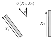
Figure 6. Two rigid rods with interaction potential $U$.

The model we are studying in Eq. (28) has no effect of shear flow and is a reversible system when $\sigma_{1}=\sigma_{2}$. In the following, we are interested in how different values of the ratio $\sigma_{2}/\sigma_{1}$ affects the transition paths. First we give the action functional form for this example. We write the path as a pair $\varphi=[\varphi_{1},\varphi_{2}]\in\mathbb{R}^{3}\times\mathbb{R}^{3}$. Denote $b(\varphi)=[b_{1}(\varphi),b_{2}(\varphi)]\in\mathbb{R}^{3}\times\mathbb{R}^{3}$ where $b_{i}(\varphi)=-\nabla V(\varphi_{i})-\nabla_{\boldsymbol{x}_{i}}U(\varphi_{1},\varphi_{2})$ corresponds to the rod $i$. The geometric action functional (20) for Eq. (28) thus has the following form

$$\hat{S}[\varphi]=\int_{0}^{1}\sqrt{\frac{\left\|b_{1}\right\|^{2}}{\sigma_{1}^{2}}+\frac{\left\|b_{2}\right\|^{2}}{\sigma_{2}^{2}}}\sqrt{\frac{\varphi_{1}^{\prime 2}}{\sigma_{1}^{2}}+\frac{\varphi_{2}^{\prime 2}}{\sigma_{2}^{2}}}-\frac{\left\langle b_{1},\varphi_{1}^{\prime}\right\rangle}{\sigma_{1}^{2}}-\frac{\left\langle b_{2},\varphi_{2}^{\prime}\right\rangle}{\sigma_{2}^{2}}\,\mathrm{d}\alpha.$$ (30)

The constraint is $\left\|\varphi_{1}\right\|=\left\|\varphi_{2}\right\|=1$.

We choose the quadratic potential as in the previous example of one rod. $V(\boldsymbol{x})=\boldsymbol{x}^{\rm T}K\boldsymbol{x}$/2. Here $K=\mbox{diag}\{\mu_{1},\mu_{2},\mu_{3}\}$ where $\mu_{1}<\mu_{2}<\mu_{3}$. Next, we show the following property of the drift flow of Eq. (28) on $\mathbb{S}^{2}\times\mathbb{S}^{2}$ for the weak strength of the interaction.

Proposition 6.

If the coupling constant $A$ in the potential Eq. (29) satisfies

$$A<\frac{1}{4}\min\limits_{i\neq j}\left|\mu_{i}-\mu_{j}\right|$$ (31)

hold, then all fixed points of the deterministic drift flow of Eq. (28) are the following $36$ points

$$(\pm\boldsymbol{e}_{i},\pm\boldsymbol{e}_{j}),~{}~{}~{}i,j=1,2,3,$$

where $\boldsymbol{e}_{i}$ is the unit eigenvector of $K$ for eigenvalue $\mu_{i}$, for instance $\boldsymbol{e}_{1}=(1,0,0)$. Moreover, the four points $(\pm\boldsymbol{e}_{1},\pm\boldsymbol{e}_{1})$ are stable (classified as sink), the four points $(\pm\boldsymbol{e}_{3},\pm\boldsymbol{e}_{3})$ are unstable (classified as source) and other fixed points are all saddles.

Proof.

It can be verified that any fixed point $(\boldsymbol{x}_{1},\boldsymbol{x}_{2})$ must satisfy the following equations

$$-K\boldsymbol{x}_{1}+2A\left\langle\boldsymbol{x}_{1},\boldsymbol{x}_{2}\right\rangle\boldsymbol{x}_{2}-2A\left\langle\boldsymbol{x}_{1},\boldsymbol{x}_{2}\right\rangle^{2}\boldsymbol{x}_{1}+(\boldsymbol{x}_{1}^{\rm T}K\boldsymbol{x}_{1})\boldsymbol{x}_{1}=0,$$ (32)

$$-K\boldsymbol{x}_{2}+2A\left\langle\boldsymbol{x}_{1},\boldsymbol{x}_{2}\right\rangle\boldsymbol{x}_{1}-2A\left\langle\boldsymbol{x}_{1},\boldsymbol{x}_{2}\right\rangle^{2}\boldsymbol{x}_{2}+(\boldsymbol{x}_{2}^{\rm T}K\boldsymbol{x}_{2})\boldsymbol{x}_{2}=0,$$ (33)

$$\left\|\boldsymbol{x}_{1}\right\|=\left\|\boldsymbol{x}_{2}\right\|=1.$$ (34)

If $\left\langle\boldsymbol{x}_{1},\boldsymbol{x}_{2}\right\rangle=0$, Eqs. (32) and (33) suggest $\boldsymbol{x}_{1}$ and $\boldsymbol{x}_{2}$ must be unit eigenvectors of $K$ corresponding to distinctive eigenvalues, respectively. It gives 24 fixed points $(\pm\boldsymbol{e}_{i},\pm\boldsymbol{e}_{j})$ for $i\neq j$ in this case.

If $\left\langle\boldsymbol{x}_{1},\boldsymbol{x}_{2}\right\rangle\neq 0$, Eqs. (32) and (33) together imply that $\left\langle\boldsymbol{x}_{1},\boldsymbol{x}_{2}\right\rangle$ $(\boldsymbol{x}_{1}^{\rm T}K\boldsymbol{x}_{1}-\boldsymbol{x}_{2}^{\rm T}K\boldsymbol{x}_{2})=0,$ or, $x_{1}^{\rm T}Kx_{1}=x_{2}^{\rm T}Kx_{2}=\lambda$. Furthermore, by considering (32) $\pm$ (33), we have $\boldsymbol{x}_{1}\pm\boldsymbol{x}_{2}$ are either zero vector or an eigenvector of $K$. The former case gives the other 12 fixed points $(\pm\boldsymbol{e}_{i},\pm\boldsymbol{e}_{i})$. The latter case that $\boldsymbol{x}_{1}\pm\boldsymbol{x}_{2}$ is an eigenvector of $K$ will eventually lead to an equality $\mu_{i}-\mu_{j}=4A\left\langle x_{1},x_{2}\right\rangle$. But since it follows $\left|\mu_{i}-\mu_{j}\right|=\left|4A\left\langle x_{1},x_{2}\right\rangle\right|\leq 4A\left\|x_{1}\right\|\left\|x_{2}\right\|=4A,$ which contradicts to condition (31), there are no other solutions.

The conclusions of the linear stability are based on the calculation of the Jacobian matrices at these fixed points. We neglect the details. ∎

In all, there are 36 different fixed points. From the above proof we know that $(\boldsymbol{e}_{i},\boldsymbol{e}_{j})$ is a fixed point even without the condition (31). If the condition (31) does not hold, there may be other fixed points and it can be shown that there are at most 60 fixed points. In our numerical calculations, we choose $K={\rm diag}\{1,3,5\},A=0.4$ to satisfy the condition (31). In addition, we always let $\sigma_{1}=1$ but allow $\sigma_{2}$ to vary.

The transition path we will study is from the initial state $(\boldsymbol{e}_{1},-\boldsymbol{e}_{1})$ to the final state $(-\boldsymbol{e}_{1},\boldsymbol{e}_{1})$, in which both rods flip over their initial directions. Since the initial and final states both lie in the $\boldsymbol{e}_{1}$-$\boldsymbol{e}_{2}$ plane for each rod, then by symmetry consideration, the transition paths, i.e., the minimizers of the action functional Eq. (30) must also lie in this plane. Our numerical calculations based on $\mathbb{S}^{2}\times\mathbb{S}^{2}$ indeed verify this fact. Therefore, we can visualize the obtained paths and interpret our results on a lower dimensional product space $\mathbb{S}^{1}\times\mathbb{S}^{1}$. It is convenient to use local coordinates $(\theta_{1},\theta_{2})\in[0,2\pi)\times[0,2\pi)$ to denote a point of the path $(\phi_{1},\phi_{2})$:

$$\phi_{1}=[\cos\theta_{1},\sin\theta_{1},0],\quad\phi_{2}=[\cos\theta_{2},\sin\theta_{2},0].$$

In this local coordinates representation, the initial and final states $(\boldsymbol{e}_{1},-\boldsymbol{e}_{1})$ and $(-\boldsymbol{e}_{1},\boldsymbol{e}_{1})$ can be written as $(\theta_{1},\theta_{2})=(0,\pi)$ and $(\pi,0)$, respectively. There are 16 fixed points on $\mathbb{S}^{1}\times\mathbb{S}^{1}$ in total. Further taking into account the spatial symmetry, we only need to focus on 4 sinks and 5 saddles for $(\theta_{1},\theta_{2})\in[0,\pi]\times[0,\pi]$, as shown in Table 1 and Figure 7. In the figure, the heteroclinic orbits between these fixed points are shown in arrowed lines. The saddle point $sa_{5}$, at the centre of the figure, is on the separatrix of all four sinks in the phase space and its unstable manifold has dimension 2. All other four saddle points have one dimensional unstable manifold for each, i.e. they are index-1 saddles.

stable points	$\mathbb{S}^{2}\times\mathbb{S}^{2}$	$(\theta_{1},\theta_{2})$	saddle points	$\mathbb{S}^{2}\times\mathbb{S}^{2}$	$(\theta_{1},\theta_{2})$
$si_{1}$	$(\boldsymbol{e}_{1},\boldsymbol{e}_{1})$	$(0,0)$	$sa_{1}$	$(\boldsymbol{e}_{2},\boldsymbol{e}_{1})$	$(\pi/2,0)$
$si_{2}$	$(\boldsymbol{e}_{1},-\boldsymbol{e}_{1})$	$(0,\pi)$	$sa_{2}$	$(\boldsymbol{e}_{1},\boldsymbol{e}_{2}$)	$(0,\pi/2)$
$si_{3}$	$(-\boldsymbol{e}_{1},\boldsymbol{e}_{1})$	$(\pi,0)$	$sa_{3}$	$(\boldsymbol{e}_{2},-\boldsymbol{e}_{1})$	$(\pi/2,\pi/2)$
$si_{4}$	$(-\boldsymbol{e}_{1},-\boldsymbol{e}_{1})$	$(\pi,\pi)$	$sa_{4}$	$(-\boldsymbol{e}_{1},\boldsymbol{e}_{2})$	$(\pi,\pi/2)$
			$sa_{5}$	$(\boldsymbol{e}_{2},\boldsymbol{e}_{2})$	$(\pi/2,\pi/2)$

Table 1. 4 sinks and 5 saddles for $(\theta_{1},\theta_{2})\in[0,\pi]\times[0,\pi]$.

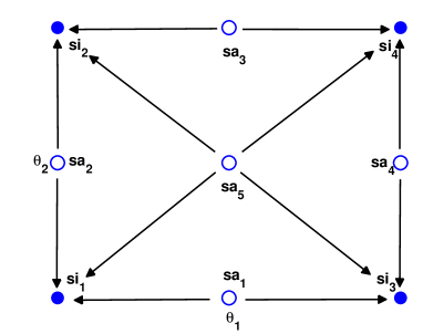
Figure 7. Fixed points in $\theta_{1}$-$\theta_{2}$ plane. Sinks are denoted by solid dots ($\bullet$) , saddles are denoted by circles ($\circ$). The arrows shows the heteroclinic orbits of the deterministic drift flow. All saddles have index 1 except that $sa_{5}$ has index 2.

The transition path we studied is from $si_{2}$ to $si_{3}$ which are two diagonal elements in Figure 7. In solving minimization problem $\inf_{\phi}\hat{S}[\phi]$, one critical issue is how to locate the global solution rather than trapped by the local ones [WZE10]. Since there is no efficient global minimization solvers (we used matlab subroutine fmincon for nonlinear optimization), the selection of initial guess of path is crucial. We utilize the information of the heteroclinic orbits in Figure 7 and propose the following five routes as our initial guesses by choosing different transition states or intermediate states:

A:

$si_{2}\to sa_{5}\to si_{3}$,

B:

$si_{2}\to sa_{2}\to sa_{5}\to si_{3}$,

C:

$si_{2}\to sa_{2}\to si_{1}\to sa_{1}\to si_{3}$,

D:

$si_{2}\to sa_{3}\to sa_{5}\to si_{3}$,

E:

$si_{2}\to sa_{3}\to si_{4}\to sa_{4}\to si_{3}$.

Then, each choice of initial guess gives a local minimum action path and the obtained minimized actions for the five solutions are plotted in Figure 8. The lowest value of these five curves gives the global minimum action.

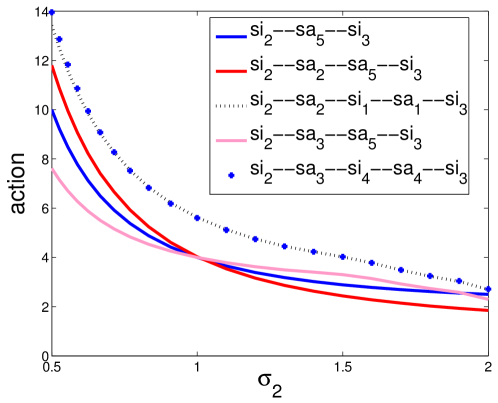
Figure 8. Numerical values of the minimal actions corresponding to five different initial guess paths by varying the diffusion coefficient $\sigma_{2}$.

When $\sigma_{1}=\sigma_{2}$, the same global solution can be achieved from initial guesses A, B and D. This global minimum action path is the diagonal line ($si_{2}\to sa_{5}\to si_{3}$) in the $\theta_{1}$-$\theta_{2}$ visualization (Figure 9(a)). However, when $\sigma_{2}\neq\sigma_{1}$, the symmetric path ($si_{2}\to sa_{5}\to si_{3}$) is not the global minimal solution; in fact, the path for the global solution will pass through index-1 saddle point $sa_{2}$ (if $\sigma_{2}>\sigma_{1}$) or $sa_{3}$ (if $\sigma_{2}<\sigma_{1}$).

Take $\sigma_{2}=1.2>\sigma_{1}=1$ as an example. The transition path corresponding to the global minimizer of the action functional is shown in the right panel of Figure 9(b). The symmetry of the transition path is broken for this case of unequal diffusion coefficients. This asymmetric path has three segments and accordingly the transition process can be understood via three stages: The first stage is from $si_{2}=(\boldsymbol{e}_{1},-\boldsymbol{e}_{1})$ to $sa_{2}=(\boldsymbol{e}_{1},\boldsymbol{e}_{2})$, where the first rod does not move much and only the second rod, which has the larger diffusion coefficient, rotates in clockwise to the vertical position $\boldsymbol{e}_{2}$; then, at the second stage which is from $sa_{2}$ to $sa_{5}=(\boldsymbol{e}_{2},\boldsymbol{e}_{2})$ , the second rod is almost still and “waits” in the state $\boldsymbol{e}_{2}$ for the first rod to move from $\boldsymbol{e}_{1}$ to $\boldsymbol{e}_{2}$. Once both rods reach the saddle state $sa_{5}$, the last state starts and both rods directly approach the final state $si_{3}$ following the heteroclinic orbit in Figure 7 without any aid from noise.

The above numerical results demonstrate a selection mechanism: the rod with a larger diffusion coefficient $\sigma$ is subject to large random perturbations with the same white noise realizations, and thus it is easier to make transition movements first. We may call this rod as an “active” rod. After this rod actively approaches a critical state ($\boldsymbol{e}_{2}$ here), it rests there, and the interaction $U(\boldsymbol{x}_{1},\boldsymbol{x}_{2})$ starts to be the main contributor to influence the system and the previously still rod (“passive” one) is attracted by $U$ from the active rod to the critical state, from where the entire system has crossed all the barriers on the route of the transition. What is unexpected here is the “sequentiality” of the two rods’ movement during the first and the second transition stages. In other words, “sequentiality” here means the relative insensitivity to the other rod when one rod is making progressive transition movement. Taking an analogy of the so-called reaction coordinate in chemical reactions, we can think of $\theta_{2}$ as an excellent candidate for reaction coordinate at the first transition stage and $\theta_{1}$ at the second stage. When we varied $\sigma_{2}$ from $1$ to $2$ ($\sigma_{1}=1$ is fixed), the numerical result shows the robustness of this set of reaction coordinates especially at the first stage from $si_{2}$ to $sa_{2}$. Refer to Figure 9(c) for the plots of 40 (global minimum action) paths for various values of $\sigma_{2}$ by equally dividing the squared $\sigma_{2}$ from $1$ to $4$.

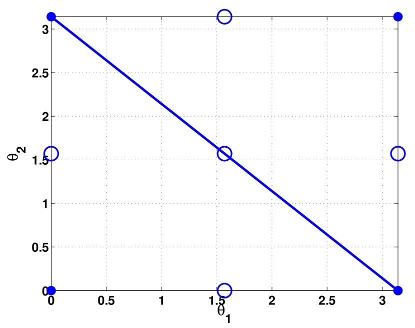
(a) $\sigma_{2}=1$

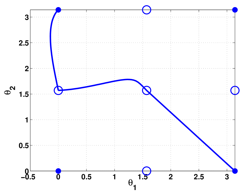
(b) $\sigma_{2}=1.2$

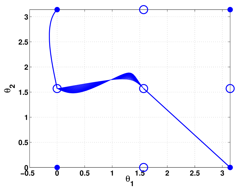
(c) $\sigma_{2}\in(1,2)$

Figure 9. Global minimum action path(s) from $si_{2}$ to $si_{3}$.

In all, when the diffusion coefficients for the two rigid rods are identical, the transition path is symmetric and both rods move simultaneously in the transitions. If one of the diffusion coefficients is adjusted, then the rod molecule with larger diffusion amplitude will initiatively move into some intermediate state, then the other will follow in the similar fashion. The unbalance of the noise amplitudes triggers an ordered process for each rod to make the transitions.

6. Outlook

So far we have studied the most probable transition pathway for the stochastic dynamics of the type (3). In this setup, the drift and diffusion terms, in particular the projection $\Pi$, are explicitly known so that the random motion does sit on the manifold $\mathcal{M}$. Another interesting but different setup is that the drift and diffusion terms are not known beforehand but left to be determined by the constraints. This situation is very common for problems in computational science. Let us illustrate this point with an example from the polymer science [DS98].

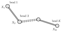
Figure 10. The schematics of the bead-rod polymer chain with $K$ beads.

Consider a bead-rod polymer chain with $K$-beads (Figure 10), being described, for instance, by the following over-damped stochastic dynamics

$$\,\mathrm{d}\boldsymbol{X}_{i}=\Big{(}\boldsymbol{u}(\boldsymbol{X}_{i})+(T_{i}\boldsymbol{n}_{i}-T_{i-1}\boldsymbol{n}_{i-1})\Big{)}\,\mathrm{d}t+\sqrt{\varepsilon}\,\mathrm{d}\boldsymbol{W}_{i},\quad i=1,2,\ldots,K$$ (35)

where $\boldsymbol{X}_{i}$ is the coordinate of the $i$th bead, $\boldsymbol{u}(\boldsymbol{X})$ is the fluid velocity at $\boldsymbol{X}$, $\boldsymbol{n}_{i}=(\boldsymbol{X}_{i+1}-\boldsymbol{X}_{i})/\|\boldsymbol{X}_{i+1}-\boldsymbol{X}_{i}\|$ for $i=1,2,\ldots,K-1$, and $T_{i}$ is the tension between the beads $i$ and $i+1$ such that the constraints

$$\|\boldsymbol{X}_{i+1}-\boldsymbol{X}_{i}\|=1,\quad i=1,2,\ldots,K-1$$ (36)

are satisfied. We take the convention that $T_{0}=0$ and $\boldsymbol{n}_{K}=0$. It is obvious that the tension $\{T_{i}\}$ play the role of the Lagrange multipliers and it is only known after solving a nonlinear system. In this case, the previously considered formulation is not sufficient.

However, the transition pathway finding problem can also be formulated based on large deviation theory. The straightforward application of the Freidlin-Wentzell theory to the system (35) and (36) gives the rate functional

$$S_{T}[\boldsymbol{\phi}]=\frac{1}{2}\sum_{i=1}^{K}\int_{0}^{T}\|\dot{\boldsymbol{\phi}}_{i}-\boldsymbol{u}(\boldsymbol{\phi}_{i})-\boldsymbol{b}_{i}\|^{2}\,\mathrm{d}t$$ (37)

such that

$$\|\boldsymbol{\phi}_{i+1}-\boldsymbol{\phi}_{i}\|=1,\quad i=1,2,\ldots,K-1,$$ (38)

where $\boldsymbol{b}_{i}=T_{i}\boldsymbol{n}_{i}-T_{i-1}\boldsymbol{n}_{i-1}$ and $\boldsymbol{n}_{i}=(\boldsymbol{\phi}_{i+1}-\boldsymbol{\phi}_{i})/\|\boldsymbol{\phi}_{i+1}-\boldsymbol{\phi}_{i}\|$. Its geometric formulation can be obtained similarly as the derivations in [HVE08]. We have

$$\hat{S}[\boldsymbol{\varphi}]=\frac{1}{2}\int_{0}^{1}\left\langle\boldsymbol{\varphi}^{\prime},\hat{\boldsymbol{p}}(\boldsymbol{\varphi},\boldsymbol{\varphi}^{\prime})\right\rangle\,\mathrm{d}\alpha$$

such that (38) is also satisfied. Here $(\hat{\boldsymbol{p}}(\boldsymbol{x},\boldsymbol{y}),\lambda)$ is the unique solution of the system

$$H(\boldsymbol{x},\hat{\boldsymbol{p}})=0,\quad H_{\boldsymbol{p}}(\boldsymbol{x},\hat{\boldsymbol{p}})=\lambda\boldsymbol{y}$$

where the Hamiltonian $H:\mathbb{R}^{3K}\times\mathbb{R}^{3K}\rightarrow\mathbb{R}$ is defined as

$$H(\boldsymbol{x},\boldsymbol{p})=\frac{1}{2}\left\langle\boldsymbol{p},\boldsymbol{p}\right\rangle+\left\langle\boldsymbol{u}(\boldsymbol{x})+\boldsymbol{b}(\boldsymbol{x}),\boldsymbol{p}\right\rangle.$$

Based on the obtained optimization problem with constraints or its relaxation form, we can compute the transition pathways correspondingly. We shall not develop the study on this point here since it is beyond the main goal of this paper. Further research on this topic will be a future study.

7. Summary

In this summary, we want to reiterate the mathematical importance of specifying how the constrained dynamical system is perturbed by noise when one intends to investigate the transition paths in such constrained systems. Here we considered the SDE whose solutions satisfy constraints, i.e., stay on $\mathcal{M}$, for any $\varepsilon$, rather than satisfy constraints in the asymptotic sense. The asymptotic limit $\varepsilon\downarrow 0$ is only applied in the large deviation result. In formulating the action functional, we take the approach of using the local projection $\Pi$ to describe the constraints and solved the issue of degeneracy brought by this projection operator in the augmented Euclidean space $\mathbb{R}^{n}$. Certainly, it is possible to use the Lagrangian multiplier to describe the constraints as mentioned in the previous section.

The constraints in the reversible case where the drift term is of gradient type and the diffusion coefficient is isotropic constant actually do not cause significant troubles in computations since the original string method still works by using the projected gradient force for each image on string: It is essentially the same as one solves the deterministic gradient flow on the manifold.

In the irreversible case, the calculation of constrained minimum action need consider the generalized inverse of the projection operator unless the diffusion coefficient is isotropic constant. Additionally, the resulting constrained optimization problem needs to be solved by carefully choosing initial guesses to find the global solution. The initial guesses in our example of rigid rod models are built on some prior understanding of the phase spaces. In our study that the liquid crystal molecules are under the influence of shear or possess unequal diffusion constants, the found global minimum action pathways reveal very interesting non-equilibrium phenomena, and these phenomena are believed to be generic in irreversible systems and deserve further investigations.

References

- [BG80] R.L. Bishop and S.I. Goldberg, Tensor analysis on manifolds, Dover Publications, New York, 1980.
- [DS98] P.S. Doyle and E.S.G. Shaqfeh, Dynamic simulation of freely-draining, flexible bead-rod chains: Start-up of extensional and shear flow, J. Non-Newtonian Fluid Mech. 76 (1998), 43–78.
- [DZ09] Q. Du and L. Zhang, A constrained string method and its numerical analysis, Comm. Math. Sci 7 (2009), 1039–1051.
- [ERVE02] W. E, W. Ren, and E. Vanden-Eijnden, String method for the study of rare events, Phys. Rev. B 66 (2002), 052301.
- [ERVE04] W. E, W. Ren, and E. Vanden-Eijnden, Minimum action method for the study of rare events, Comm. Pure Appl. Math. 57 (2004), 637–656.
- [FW98] M.I. Freidlin and A.D. Wentzell, Random perturbations of dynamical systems, 2nd ed., Grundlehren der mathematischen Wissenschaften, Springer-Verlag, New York, 1998.
- [Hsu02] E.P. Hsu, Stochastic analysis on manifolds, American Mathematical Society, Providence, Rode Island, 2002.
- [HVE08] M. Heymann and E. Vanden-Eijnden, The geometric minimum action method: a least action principle on the space of curves, Comm. Pure Appl. Math. 61 (2008), 1052–1117.
- [Kra40] H.A. Kramers, Brownian motion in a field of force and the diffusion model of chemical reactions, Physica 7 (1940), 284–304.
- [LL76] L.D. Landau and E.M. Lifshitz, Mechanics, 3rd ed., Course of Theoretical Physics, Butterworth-Heinemann, 1976.
- [LZZ04] T. Li, P. Zhang, and X. Zhou, Analysis of 1 + 1 dimensional stochastic models of liquid crystal polymer flows, Comm. Math. Sci. 2 (2004), no. 2, 295–316.
- [MS93] R.S. Maier and D.L. Stein, Escape problem for irreversible systems, Phys. Rev. E 48 (1993), no. 2, 931–938.
- [Ött96] H.C. Öttinger, Stochastic processes in polymeric fluids: Tools and examples for developing simulation algorithms, Springer-Verlag, Berlin Heidelberg, 1996.
- [Var84] S.R.S. Varadhan, Large deviations and applications, CBMS-NSF Regional Conference Series in Applied Mathematics, 46, SIAM, Philadelphia, 1984.
- [WZE10] X. Wan, X. Zhou, and W. E, Study of noise-induced transition and the exploration of the configuration space for the Kuromoto-Sivachinsky equation using the minimum action method, nonlinearity 23 (2010), no. 3, 475–493.
- [ZRE08] X. Zhou, W. Ren, and W. E, Adaptive minimum action method for the study of rare events, J. Chem. Phys. 128 (2008), no. 10, 104111.