Indexing Cost Sensitive Prediction

Abstract

Predictive models are often used for real-time decision making. However, typical machine learning techniques ignore feature evaluation cost, and focus solely on the accuracy of the machine learning models obtained utilizing all the features available. We develop algorithms and indexes to support cost-sensitive prediction, i.e., making decisions using machine learning models taking feature evaluation cost into account. Given an item and a online computation cost (i.e., time) budget, we present two approaches to return an appropriately chosen machine learning model that will run within the specified time on the given item. The first approach returns the optimal machine learning model, i.e., one with the highest accuracy, that runs within the specified time, but requires significant up-front precomputation time. The second approach returns a possibly sub-optimal machine learning model, but requires little up-front precomputation time. We study these two algorithms in detail and characterize the scenarios (using real and synthetic data) in which each performs well. Unlike prior work that focuses on a narrow domain or a specific algorithm, our techniques are very general: they apply to any cost-sensitive prediction scenario on any machine learning algorithm.

1 Introduction

Predictive models are ubiquitous in real-world applications: ad-networks predict which ad the user will most likely click on based on the user’s web history, Netflix uses a user’s viewing and voting history to pick movies to recommend, and content moderation services decide if an uploaded image is appropriate for young children. In these applications, the predictive model needs to process the input data and make a prediction within a bounded amount of time, or risk losing user engagement or revenue [4, 13, 34].

Unfortunately, traditional feature-based classifiers take a one-model-fits all approach when placed in production, behaving the same way regardless of input size or time budget. From the classifier’s perspective, the features used to represent an input item have already been computed, and this computation process is external to the core task of classification. This approach isolates and simplifies the core task of machine learning, allowing theorists to focus on tasks like quick learning convergence and accuracy. But it leaves out many important aspects of production systems can be just as important as accuracy, such as tunable prediction speed.

In reality, the cost of computing features can easily dominate prediction time. For example, a content moderation application may use a support-vector machine to detect inappropariate images. At runtime, SVMs need only perform a single dot-product between a feature vector and pre-computed weight vector. But computing the feature vector may require several scans of an image which may take longer than an alotted time budget.

If feature computation is the dominating cost factor, one might intuitively accomodate time constraints by computing and using only a subset of features available. But selecting which subset to use at runtime—and guaranteeing that a model is available that was trained on that subet—is made challenging by a number of factors. Features vary in predictive power, e.g. skin tone colors might more accurately predict inappropriate images than image size. They also vary in prediction cost, e.g. looking up the image size is much faster than computing a color histogram over an entire image. This cost also varies with respect to input size—the size feature may be $O(1)$, stored in metadata, while the histogram may be $O(r\times c)$. Finally for any $n$ features, $2^{n}$ distinct subsets are possible, each with their aggregate predictive power and cost, and each potentially requiring its own custom training run. As the number of potential features grows large, training a model for every possible subset is clearly prohibitively costly. All of these reasons highlight why deploying real-time prediction, while extremely important, is a particularly challenging problem.

Existing strategies of approaching this problem (see Section 6) tend to be either tightly coupled to a particular prediction task or to a particular mathematical model. While these approaches work for a particular problem, they are narrow in their applicability: if the domain (features) change or the machine learning model is swapped for new one (e.g., SVM for AdaBoost), the approach will no longer work.

In this paper, we develop a framework for cost-sensitive real-time classification as a wrapper over “off-the-shelf” feature-based classifiers. That is, given an item that needs to be classified or categorized in real time and a cost (i.e., time) budget for feature evaluation, our goal is to identify features to compute in real time that are within the budget, identify the appropriate machine learning model that has been learned in advance, and apply the model on the extracted features.

We take a systems approach by decoupling the problem of cost-sensitive prediction from the problem of machine learning in general. We present an algorithm for cost sensitive prediction that operates on any feature-based machine learning algorithm as a black box. The few assumptions it makes reasonably transfer between different feature sets and algorithms (and are justified herein). This decoupled approach is attractive for the same reason that machine learning literature did not originally address such problems: it segments reasoning about the core tasks of learning and prediction from system concerns about operationalizing and scaling. Additionally, encapsulating the details of classification as we do ensures advances in machine learning algorithms and feature engineering can be integrated without change to the cost-sensitivity apparatus.

Thus, our focus in this paper is on systems issues underlying this wrapper-based approach, i.e., on intelligent indexing and pruning techniques to enable rapid online decision making and not on the machine learning algorithms themselves. Our contribution is two approaches to this problem as well as new techniques to mitigate the challenges of each approach. These two approaches represents two ends of a continuum of approaches to tackle the problem of model-agnostic cost sensitivity:

• Our Poly-Dom approach yields optimal solutions but requires significant offline pre-computation,

• Our Greedy approach yields relatively good solutions but does not require significant offline pre-computation.

First, consider the Greedy approach: Greedy, and its two sub-variants Greedy-Acc and Greedy-Cost (described in Section 4), are all simple but effective techniques adapted from prior work by Xu et al. [45], wherein the technique only applied to a sub-class of SVMs [15]. Here, we generalize the techniques to apply to any machine learning classiciation algorithm as a black box. Greedy is a “quick and dirty” technique that requires little precomputation, storage and retrieval, and works well in many settings.

Then, consider our Poly-Dom approach, which is necessary whenever accuracy is paramount, a typical scenario in critical applications like credit card fraud detection, system performance monitoring, and ad-serving systems. In this approach, we conceptually store, for each input size, a skyline of predictive models along the axes of total real-time computation cost vs. accuracy. Then, given an input of that size, we can simply pick the predictive model along the skyline within the total real-time computation cost budget, and then get the best possible accuracy.

However, there are many difficulties in implementing this skyline-based approach:

• Computing the skyline in a naive fashion requires us to compute for all $2^{|\cal{F}|}$, subsets of features (where $\cal{F}$ is the set of all features) the best machine learning algorithm for that set, and the total real-time computation time (or cost). If the number of features is large, say in the 100s or the 1000s, computing the skyline is impossible to do, even with an unlimited amount of time offline. How do we intelligently reduce the amount of precomputation required to find the skyline?

• The skyline, once computed, will require a lot of storage. How should this skyline be stored, and what index structures should we use to allow efficient retrieval of individual models on the skyline?

• Computing and storing the skyline for each input size is simply infeasible: an image, for instance, can vary between 0 to 70 Billion Pixels (the size of the largest photo on earth [1]), we simply cannot store or precompute this much information. What can we do in such a case?

To deal with the challenges above, Poly-Dom use a dual-pronged solution, with two precomputation steps:

• Feature Set Pruning: We develop a number of pruning techniques that enable us to minimize the number of feature sets for which we need to learn machine learning algorithms. Our lattice pruning techniques are provably correct under some very reasonable assumptions, i.e., they do not discard any feature sets if those feature sets could be potentially optimal under certain input conditions. We find that our pruning techniques often allow us to prune up to 90% of the feature sets.

• Polydom Index: Once we gather the collection of feature sets, we develop an index structure that allows us to represent the models learned using the feature sets in such a way that enables us to perform efficient retrieval of the optimal machine learning model given constraints on cost and input size. This index structure relies on reasoning about polynomials that represent cost characteristics of feature sets as a function of input size.

Overall, our approach offers a systems perspective to an increasingly important topic in the deployment of machine learning systems. The higher-level goal is to isolate and develop the mechanisms for storage and delivery of cost-sensitive prediction without having to break the encapsulation barrier that should surround the fundamental machinery of machine learning. Our techniques could be deployed alongside the existing algorithms in a variety of real-time prediction scenarios, including:

• An ad system needs to balance between per-user ad customization and latency on the small scale, and allocate computational resources between low-value and high-value ad viewers on the aggregate scale.

• Cloud-based financial software needs to run predictive models on portfolios of dramatically different input size and value. A maximum latency on results may be required, but the best possible model for each time and input size pairing is financially advantageous.

• An autopilot system in an airplane has a limited time to respond to an error. Or more broadly, system performance monitors in a variety of industrial systems have fixed time to decide whether to alert a human operator of a failure.

• A mobile sensor has limited resources to decide if an error needs to be flagged and sent to the central controller.

In the rest of the paper, we will first formally present our problem variants in Section 2, then describe our two-pronged Poly-Dom solution in Section 3 and our “quick and dirty” Greedy solution in Section 4, and finally present our experiments on both synthetic and real-world datasets in Section 5.

2 Problem Description

We begin by describing some notation that will apply to the rest of the paper, and then we will present the formal statement of the problems that we study.

Our goal is to classify an item (e.g., image, video, text) $x$ during real-time. We assume that the size of $x$, denoted $|x|$, would be represented using a single number or dimension $n$, e.g., number of words in the text. Our techniques also apply to the scenario when the size can be represented using a vector of dimensions: for example, (length, breadth), for an image; however, for ease of exposition, we focus on the single dimension scenario. The entire set of features we can evaluate on $x$ is ${\cal F}$; each individual feature is denoted $f_{i}$, while a non-empty set of features is denoted $F_{j}$.

We assume that we have some training data, denoted ${\cal T}$, wherein every single feature $f_{i}\in{\cal F}$ is evaluated for each item. Since training is done offline, it is not unreasonable to expect that we have the ability to compute all the features on each item. In addition, we have some testing data, denoted ${\cal T^{\prime}}$, where once again every single feature is evaluated for each item. We use this test data to estimate the accuracy of the machine learning models we discover offline.

Cost Function: We assume that evaluating a feature on an item $x$ depends only on the feature that is being computed, and the size of the item $|x|$. We denote the cost of computing $f_{i}$ on $x$ as: $c(f_{i},|x|)$. We can estimate $c(f_{i},n)$ during pre-processing time by running the subroutine corresponding to feature evaluation $f_{i}$ on varying input sizes. Our resulting expression for $c(f_{i},n)$ could either be a constant (if it takes a fixed amount of time to evaluate the feature, no matter the size), or could be a function of $n$, e.g., $3n^{2}+50$, if evaluating a feature depends on $n$.

Then, the cost of computing a set of features $F_{i}$ on $x$ can be computed as follows:

$$c(F_{i},|x|)=\sum_{f\in F_{i}}c(f,|x|)$$ (1)

We assume that each feature is computed independently, in sequential order. Although there may be cases where multiple features can be computed together (e.g., multiple features can share scans over an image simultaneously), we expect that users provide the features as “black-box” subroutines and do not want to place additional burden by asking users to provide subroutines for combinations of features as well. That said, our techniques will equally well apply to the scenario when our cost model is more general than Equation 1, or if users have provided subroutines for generating multiple feature values simultaneously (e.g., extracting a word frequency vector from a text document).

Accuracy Function: We model the machine learning algorithm (e.g., SVM, decision tree, naive-bayes) as a black box function supplied by the user. This algorithm takes as input the entire training data ${\cal T}$, as well as a set of features $F_{i}$, and outputs the best model ${\cal M}(F_{i})$ learned using the set of features $F_{i}$. We denote the accuracy of ${\cal M}(F_{i})$ inferred on the testing data ${\cal T^{\prime}}$ as $a(F_{i})$, possibly using k-fold cross-validation. We assume that the training data is representative of the items classified online (as is typical), so that the accuracy of the model ${\cal M}(F_{i})$ is still $a(F_{i})$ online.

Note that we are implicitly assuming that the accuracy of the classification model only depends on the set of features inferred during test time, and not on the size of the item. This assumption is typically true in practice: whether or not an image needs to be flagged for moderation is independent of the size of the image.

Characterizing a Feature Set: Since we will be dealing often with sets of features at a time, we now describe what we mean by characterizing a feature set $F_{i}$. Overall, given $F_{i}$, as discussed above, we have a black box that returns

• a machine learning model learned on some or all the features in $F_{i}$, represented as ${\cal M}(F_{i})$.

• $a(F_{i})$, i.e., an estimate of the accuracy of the model ${\cal M}(F_{i})$ on test data ${\cal T^{\prime}}$.

In addition, we can estimate $c(F_{i},n)$, i.e., the cost of extracting the features to apply the model at test time as a function of the size of the item $n$. Note that unlike the last two quantities, this quantity will be expressed in symbolic form. For example, $c(F_{i},n)$ could be an expression like $3n^{2}+4n\log n+7n$.

Characterizing a feature set $F_{i}$ thus involves learning all three quantities above for $F_{i}$: ${\cal M},a,c$. For the rest of the paper, we will operate on feature sets, implicitly assuming that a feature set is characterized by the best machine learning model for that feature set, an accuracy value for that model, and a cost function.

Problem Statements: The most general version of the problem is when $c$ (i.e., the cost or time constraint) and the size $n$ of an item $x$ are not provided to us in advance:

Problem 1 (Prob-General)

Given ${\cal F},{\cal T,T^{\prime}}$ at preprocessing time, compute classification models and indexes such that the following task can be completed at real-time:

• Given $x,|x|=n$, and a cost constraint $c$ at real time, identify a set $F_{i}\in{\cal F^{\prime}}=\{F\subseteq{\cal F}\ |\ c(F,n)\leq c\}$ such that $\forall_{F\in{\cal F^{\prime}}}\alpha\times a(F_{i})\geq a(F)$ and return ${\cal M}(F_{i})(x)$.

That is, our goal is to build classification models and indexes such that given a new item at real time, we select a feature set $F_{i}$ and the corresponding machine learning model ${\cal M}(F_{i})$ that both obeys the cost constraint, and is within $\alpha\geq 1\times$ of the best accuracy among all feature sets that obey the cost constraint. The reason we care about $\alpha>1$ is that, in contrast to a hard cost constraint, a slightly lower accuracy is often acceptable as long as the amount of computation required for computing, storing, and retrieving the appropriate models is manageable. We will consider $\alpha=1$, i.e., the absolute best accuracy, as a special case; however, for most of the paper, we will consider the more general variants.

There are two special cases of the general problem that we will consider. The first special case considers the scenario when the input size is provided up-front, e.g., when Yelp fixes the size of profile images uploaded to the website that need to be moderated.

Problem 2 (Prob-$n_{0}$-Fixed)

Given ${\cal F},{\cal T,T^{\prime}}$ and a fixed $n_{0}$ at preprocessing time, compute classification models and indexes such that the following task can be completed at real-time:

• Given $x,|x|=n_{0}$, and a cost constraint $c$ at real time, identify the set $F_{i}\in{\cal F^{\prime}}=\{F\subseteq{\cal F}\ |\ c(F,n_{0})\leq c\}$ such that $\forall_{F\in{\cal F^{\prime}}}\alpha\times a(F_{i})\geq a(F)$ and return ${\cal M}(F_{i})(x)$.

We also consider the version where $c_{0}$ is provided in advance but the item size $n$ is not, e.g., when an aircraft needs to respond to any signals within a fixed time.

Problem 3 (Prob-$c_{0}$-Fixed)

Given $c_{0},{\cal F},{\cal T,T^{\prime}}$ at preprocessing time, compute classification models and indexes such that the following task can be completed at real-time:

• Given $x,|x|=n$, at real time, identify the set $F_{i}\in{\cal F^{\prime}}=\{F\subseteq{\cal F}\ |\ c(F,n)\leq c_{0}\}$ such that $\forall_{F\in{\cal F^{\prime}}}\alpha\times a(F_{i})\geq a(F)$ and return ${\cal M}(F_{i})(x)$.

Reusing Skyline Computation is Incorrect: We now argue that it is not sufficient to simply compute the skyline of classification models for a fixed item size and employ that skyline for all $n,c$. For the following discussion, we focus on $\alpha=1$; the general $\alpha$ case is similar. Given a fixed $n=n_{0}$, we define the $n_{0}-$skyline as the set of all feature sets that are undominated in terms of cost and accuracy (or equivalently, error, which is $1-$ accuracy). A feature set $F_{i}$ is undominated if there is no feature set $F_{j}$, where $c(F_{j},n_{0})<c(F_{i},n_{0})$ and $a(F_{i})\leq a(F_{j})$, and no feature set $F_{j}$ where $c(F_{j},n_{0})\leq c(F_{i},n_{0})$ and $a(F_{i})<a(F_{j})$. A naive strategy is to enumerate each feature set $F\subseteq{\cal F}$, and characterize each $F$ by its cross-validation accuracy and average extraction cost over the training dataset. Once the feature sets are charcterized, iterate through them by increasing cost, and keep the feature sets whose accuracy is greater than any of the feature sets preceeding it. The resulting set is the $n_{0}-$skyline. However, it is every expensive to enumerate and characterize all feature sets (especially when the number of features is large), and one of our key contributions will be to avoid this exhaustive enumeration. But for the purposes of discussion, let us assume that we have the $n_{0}-$skyline computed. Note that the skyline feature sets are precisely the ones we need to consider as possible solutions during real-time classification for $n=n_{0}$ for various values of $c_{0}$.

Then, one approach to solving Problem 1 could be to simply reuse the $n_{0}$-skyline for other $n$. However, this approach is incorrect, as depicted by Figure 1. Figure 1 depicts the cost and error of each feature set and the error vs. cost skyline curve for $n=n_{0}$, while Figure 1 depicts what happens when $n$ changes from $n_{0}$ to a larger value $n_{1}$ (the same holds when the value changed to a smaller value): as can be seen in the figure, different feature sets move by different amounts, based on the cost function $c(F_{i},n)$. This is because different polynomials behave differently as $n$ is varied. For instance, $2n^{2}$ is less than $3n+32$ when $n$ is small, however it is significantly larger for big values of $n$. As a result, a feature set which was on the skyline may now no longer be on the skyline, and another one that was dominated could suddenly become part of the skyline.

Figure 1: (a) Offline computation of all $F$. (b) Points skew across the cost axis as $n$ changes.

Learning Algorithm Properties: We now describe a property about machine learning algorithms that we will leverage in subsequent sections. This property holds because even in the worst case, adding additional features simply gives us no new useful information that can help us in classification.

Axiom 2.1 (Information-Never-Hurts)

If $F_{i}\subset F_{j}$, then $a(F_{i})\leq a(F_{j})$

While this property is known by the machine learning community to be anecdotally true [11], we experimentally validate this in our experiments. In fact, even if this property is violated in a few cases, our Poly-Dom algorithm can be made more robust by taking that into account, as we will see in Section 3.1

3 Poly-Dom Solution

Our solution follows three steps:

• Feature Set Pruning: First, we will start by constructing what we call as a candidate set, that is, the set of all feature sets (and corresponding machine learning models) that will be solutions to Problem 1. As a side effect, we will find a solution to Problem 2. The candidate set will be a carefully constructed superset of the skyline feature sets, so that we do not discard any feature sets that could be useful for any $n$. We will describe this in Section 3.1.

• Polydom Index Construction: In Section 3.2, we describe a new data-structure for Problem 1, called the poly-dominance index, which compactly represents the candidate set and allows it to be indexed into given a specific item size $n$ and budget $c$ during query time. In particular, we would like to organize the candidate set so that it can be efficiently probed even for large candidate sets size.

• Online Retrieval: Lastly, we describe how the poly-dominance index is accessed during query time in Section 3.3.

3.1 Offline: Constructing the Candidate Set

We will construct the candidate set using a bi-directional search on the lattice of all subsets of features, depicted in Figure 2.

When a sequence of features is listed, this sequence corresponds to the feature set containing those features. In the figure, feature sets are listed along with their accuracies (listed below the feature set). An edge connect two features sets that differ in one feature. For now, ignore the symbols $\star,\dagger$, we will describe their meaning subsequently. The feature set corresponding to $\cal F$ is depicted at the top of the lattice, while the feature set corresponding to the empty set is depicted at the bottom. The feature sets in between have $0$ to $|\cal F|$ features. In the following we use feature sets and nodes in the lattice interchangably.

Bidirectional Search: At one extreme, we have the empty set $\{\}$, and at the other extreme, we have ${\cal F}$. We begin by learning and characterizing the best machine learning model for $F=\{\}$, and for $F={\cal F}$: i.e., we learn the best machine learning model, represented as ${\cal M}(F)$, and learn the accuracy $a(F)$ (listed below the node) and $c(F,n)$ for the model We call this step expanding a feature set, and a feature set thus operated on is called an expanded feature set.

At each round, we expand the feature sets in the next layer, in both directions. We stop once we have expanded all nodes. In our lattice in Figure 2, we expand the bottom and top layer each consisting of 1 node, following which, we expand the second-to-bottom layer consisting of 4 nodes, and the second-to-top layer again consisting of 4 nodes, and then we finally expand the middle layer consisting of 6 nodes.

Figure 2: Lattice: $\star$ indicates the nodes that will be expanded for $\alpha=1$; $\dagger$ indicates the nodes that will be expanded for $\alpha=1.1$

However, notice that the total number of nodes in the lattice is $2^{|\cal F|}$, and even for relatively small ${\cal F}$, we simply cannot afford to expand all the nodes in the lattice. Therefore, we develop pruning conditions to avoid expanding all the nodes in the lattice. Note that all the pruning conditions we develop are guaranteed to return an accurate solution. That is, we do not make approximations at any point that take away the optimality of the solution.

Dominated Feature Sets: We now define what we mean for a feature set to dominate another.

Definition 3.1 (dominance)

A feature set $F_{i}$ dominates a feature set $F_{j}$ if $\forall n,$ $c(F_{i},n)$ $\leq c(F_{j},n)$ and $\alpha\times a(F_{i})\geq a(F_{j})$

As an example from Figure 2, consider node $f_{3}f_{4}$ and $f_{2}f_{3}f_{4}$ on the right-hand extreme of the lattice: the accuracies of both these feature sets is the same, while the cost of $f_{2}f_{3}f_{4}$ is definitely higher (since an additional feature $f_{2}$ is evaluated). Here, we will always prefer to use $f_{3}f_{4}$ over $f_{2}f_{3}f_{4}$, and as a result, $f_{2}f_{3}f_{4}$ is dominated by $f_{2}f_{3}$.

Overall, a feature set $F_{j}$ that is dominated is simply not under consideration for any $n$, because it is not going to be the solution to Problems 1, 2, or 3, given that $F_{i}$ is a better solution. We formalize this as a theorem:

Theorem 3.2

A feature set that is dominated cannot be the solution to Problems 1, 2, or 3 for any $n$.

Given the property above, we need to find domination rules that allow us to identify and discard dominated feature sets. In particular, in our lattice, this corresponds to not expanding feature sets.

Pruning Properties: Our first property dictates that we should not expand a feature set that is strictly “sandwiched between” two other feature sets. It can be shown that any such feature set is dominated, and therefore, using Theorem 3.2, can never be a solution to any of the problems listed in the previous section.

Property 3.3 (Sandwich-Property)

If $F_{i}\subset F_{k}$, and $\alpha\times a(F_{i})\geq a(F_{k})$, then no $F_{j}$ such that $F_{i}\subset F_{j}\subset F_{k}$, needs to be expanded.

Intuitively, if there is a feature set $F_{i}$ that dominates an $F_{j}$, while $F_{i}\subset F_{j}$, then all other feature sets betweeen $F_{i}$ and $F_{j}$ are also dominated. Consider Figure 2, with $\alpha=1$, let $F_{i}=f_{3}$, and $F_{k}=f_{2}f_{3}f_{4}$, since $a(F_{i})=a(F_{k})$, feature sets $F_{j}$ corresponding to $f_{2}f_{3}$ and $f_{3}f_{4}$ need not be expanded: in the figure, both these feature sets have precisely the same accuracy as $f_{3}$, but have a higher cost.

In Figure 2 once again for $\alpha=1$, let us consider how many expansions the previous property saves us while doing bidirectional search: We first expand ${\cal F}$ and $\{\}$, and then we expand all nodes in the second-to-top layer and the second-to-bottom layer. Then, from the next layer, $f_{2}f_{3}$ and $f_{3}f_{4}$ will not be expanded (using the argument from the previous paragraph), while the rest are expanded. Thus, we save two expansions. The expanded nodes in the lattice are denoted using $\star$s.

Now, on changing $\alpha$ slightly, the number of evaluations goes down rapidly. The nodes expanded in this case are denoted using a $\dagger$. Let us consider $\alpha=1.1$. Once again, nodes in the top two and bottom two layers are expanded. However, only $f_{1}f_{2}$ in in the middle layer needs to be expanded. This is because:

• $f_{1}f_{3}$ and $f_{1}f_{4}$ are sandwiched between $f_{1}$ and $f_{1}f_{3}f_{4}$

• $f_{2}f_{3}$ and $f_{2}f_{4}$ are sandwiched between $f_{2}$ and $f_{2}f_{3}f_{4}$

• $f_{2}f_{3}$ and $f_{3}f_{4}$ are sandwiched between $f_{3}$ and $f_{2}f_{3}f_{4}$

The previous property is hard apply directly (e.g., before expanding every feature set we need to verify if there exists a pair of feature sets that sandwich it). Next, we describe a property that specifies when it is safe to stop expanding all non-expanded ancestors of a specific node.

Property 3.4 (Covering-Property)

If $F_{i}\subset F_{k_{i}},\forall i\in 1\ldots r$ such that $\cup_{i\in 1\ldots r}F_{k_{i}}={\cal F}$, and $\alpha\times a(F_{i})\geq a(F_{k_{i}}),\forall i\in 1\ldots r$, then no feature set sandwiched between $F_{i}$ and $F_{k_{i}}$ needs to be expanded.

This property states if any set of feature sets $F_{k_{i}}$ 1) contain $F_{i}$, 2) in aggregate covers all the features in ${\cal F}$ and 3) are dominated by $F_{i}$, then all feature sets between $F_{i}$ and $F_{k_{i}}$ do not need to be expanded. The inverse property for pruning descendents also holds.

We use this property to extend the bidirectional search with an additional pruning step. Let the top frontier ${\cal F}_{top}$ be the set of feature sets expanded from the top for which no child feature set has been expanded, and let ${\cal F}_{bot}$ be similarly defined from the bottom. By directly applying the Covering-Property, we can prune the parents of $F\in{\cal F}_{bot}$ if $\forall F^{\prime}\in{\cal F}_{top}\ F\subseteq F^{\prime}$, $F$ dominates $F^{\prime}$. We can similarly use the inverse of the property to prune feature sets in the top frontier.

Properties of Expanded Nodes: We have the following theorem, that is a straightforward consequence of Property 3.3:

Theorem 3.5

The set of expanded nodes form a superset of the skyline nodes for any $n$.

In figure 2, the set of expanded nodes (denoted by $\star$ for $\alpha=1$ and $\dagger$ for $\alpha=1.1$) are the ones relevant for any $n$.

Candidate Nodes: Given the expanded set of nodes, two properties to allow us to prune away some of the expanded but dominated nodes to give the candidate nodes. Both these properties are straightforward consequences of the definition of dominance.

Property 3.6 (Subset Pruning-Property)

If $F_{i}\subset F_{k}$, and $\alpha\times a(F_{i})\leq a(F_{k})$, then $F_{k}$ does not need to be retained as a candidate

For instance, even though $f_{2}f_{3}f_{4}$ and $f_{3}$ are both expanded, $f_{2}f_{3}f_{4}$ does not need to be retained as a candidate node when $f_{3}$ is present (for any $\alpha$); also, $f_{1}f_{3}f_{4}$ does not need to be retained as a candidate node when $f_{1}$ is present for $\alpha=1.1$.

The next property is a generalization of the previous, when we have a way of evaluating polynomial dominance.

Property 3.7 (Poly-Dom Pruning-Property)

If $c(F_{i},x)$ $<c(F_{k},x),\forall x\geq 0$, and $\alpha\times a(F_{i})\leq a(F_{k})$, then $F_{k}$ does not need to be retained as a candidate

The next theorem states that we have not made any incorrect decisions until this point, i.e., the set of candidate nodes includes all the nodes that are solutions to Problems 1, 2, 3 for all $n$.

Theorem 3.8

The set of candidate nodes form a superset of the skyline nodes for any $n$.

Algorithm: The pseudocode for the algorithm can be found in the appendix split into: Algorithm 2 (wherein the lattice is traversed and the nodes are expanded) and Algorithm 1 (wherein the dominated expanded nodes are removed to give the candidate nodes).

In brief, Algorithm 2 maintains two collections: $\sf{frontierTop}$ and $\sf{frontierBottom}$, which is the frontier (i.e., the boundary) of already expanded nodes from the top and bottom of the lattice respectively. The two collections $\sf{activeTop}$ and $\sf{activeBottom}$ contain the next set of nodes to be expanded. When a node is expanded, its children in the lattice are added to $\sf{activeTop}$ if the node is expanded “from the top”, while its parents in the lattice are added to $\sf{activeBottom}$ if the node is expanded “from the bottom”.

Note that there may be smart data structures we could use to check if a node is sandwiched or not, or when enumerating the candidate set. Unfortunately, the main cost is dominated by the cost for expanding a node (which involves training a machine learning model given a set of features and estimating its accuracy), thus these minor improvements do not improve the complexity much.

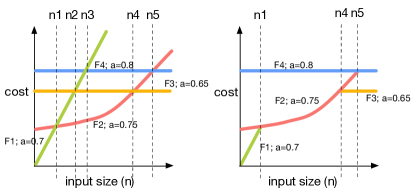
Figure 3: Incremental Poly-Dom Creation

Discussion: When the number of features in $\cal{F}$ are in the thousands, the lattice would be massive. In such cases, even the number of expanded nodes can be in the millions. Expanding each of these nodes can take a significant time, since we would need to run our machine learning algorithm on each node (i.e., feature set). In such a scenario, we have two alternatives: (a) we apply a feature selection algorithm [32] that allows us to bring the number of features under consideration to a smaller, more manageable number, or; (b) we apply our pruning algorithm in a progressive modality. In this modality, a user provides a precomputation pruning cost budget, and the pruning algorithm picks the “best $\alpha$” to meet the precomputation cost budget (i.e., the smallest possible $\alpha$ for which we can apply the lattice pruning algorithm within the precomputation cost budget.) The approach is the following: we start with a large $\alpha$ (say 2), and run the lattice pruning algorithm. Once complete, we can reduce $\alpha$ by a small amount, and rerun the lattice pruning algorithm, and so on, until we run out of the precomputation cost budget. We can make use of the following property:

Property 3.9

The nodes expanded for $\alpha_{1},1\leq\alpha_{1}<\alpha_{2}\leq 2$ is a superset of the nodes expanded for $\alpha_{2}$.

Thus, no work that we do for larger $\alpha$s are wasted for smaller $\alpha$s: as a result, directly using the $\alpha$ that is the best for the precomputation cost budget would be equivalent to the above procedure, since the above procedure expands no more nodes than necessary.

Anti-Monotonicity: Note that there may be practical scenarios where the assumption of monotonicity, i.e., Axiom 2.1, does not hold, but instead, a relaxed version of monotonicity holds, that is,

Axiom 3.10 (Information-Never-Hurts-Relaxed)

If $F_{i}\subset F_{j}$, then $a(F_{i})\leq a(F_{j})+e$

Here, if $F_{i}$ is a subset of $F_{j}$, then $a(F_{i})$ cannot be larger than $a(F_{j})+e$. Intuitively, the violations of monotonicity, if any are small—smaller than $e$ (we call this the error in the monotonicity.) Note that when $e=0$, we have Axiom 2.1 once again.

In such a scenario, only the lattice construction procedure is modified by ensuring that we do not prematurely prune away nodes (say, using the sandwich property) that can still be optimal. We use the following modified sandwich property:

Property 3.11 (Sandwich-Property-Relaxed)

If $F_{i}\subset F_{k}$, and $\alpha\times(a(F_{i})-e)\geq a(F_{k})$, then no $F_{j}$ such that $F_{i}\subset F_{j}\subset F_{k}$, needs to be expanded.

With the above property, we have a more stringent condition, i.e., that $\alpha\times(a(F_{i})-\delta)$ and not simply $\alpha\times a(F_{i})$ has to be greater than $a(F_{k})$. As a result, fewer pairs of nodes $i,k$ qualify, and as a result, fewer nodes $j:F_{i}\subset F_{j}\subset F_{k}$ are pruned without expansion.

Subsequently, when deciding whether to remove some of the expanded nodes to give candidate nodes, we have the true accuracies of the expanded nodes, we no longer need to worry about the violations of monotonicity.

3.2 Offline: Constructing the Index

We begin by collecting the set of candidate nodes from the previous step. We denote the set of candidate nodes as ${\cal C},|{\cal C}|=k$. We now describe how to construct the poly-dom index.

Alternate Visualization: Consider an alternate way of visualizing the set of candidate nodes, depicted in Figure 3(left). Here, we depict the cost $c(F_{i},n)$ for each of the candidate nodes, as a function of $n$. Also labeled with each cost curve is the accuracy. Recall that unlike cost, the accuracy stays constant independent of the input size $n$. We call each of the curves corresponding to the candidate nodes as candidate curves. We depict in our figure four candidate curves, corresponding to feature sets $F_{1},F_{2},F_{3},F_{4}$. In the figure, we depict five ‘intersection points’, where these candidate curves cross each other. We denote, in ascending order, the intersection points, as $n_{1}<\ldots<n_{r}$. In Figure 3(left), $r=5$. It is easy to see that the following holds:

Lemma 3.12

For all intersection points $n_{1}<\ldots<n_{r}$ between candidate curves, storing the skyline for the following ranges $(-\infty,n_{1}),$ $[n_{1},n_{2}),$ $\ldots,$ $[n_{r-1},n_{r}),$ $[n_{r},\infty)$ is sufficient for Problems 1,2, 3, since for any such range, the skyline is fixed.

For $(-\infty,n_{1})$, $F_{4}$ has accuracy 0.8, $F_{3}$ has accuracy 0.65, $F_{2}$ has accuracy 0.76, and $F_{1}$ has accuracy 0.7. The skyline of these four candidate sets for $n<n_{1}$ is $F_{4},F_{2},F_{1}$; $F_{3}$ is dominated by $F_{2}$ and $F_{1}$ both of which have lower cost and higher accuracy.

The lemma above describes the obvious fact that the relationships between candidate curves (and therefore nodes) do not change between the intersection points, and therefore, we only need to record what changes at each intersection point. Unfortunately, with $r$ candidate curves, there can be as many as $r^{2}$ intersection points.

Thus, we have a naive approach to compute the index that allows us to retrieve the optimal candidate curve for each value of $n_{0},c_{0}$:

• for each range, we compute the skyline of candidate nodes, and maintain it ordered on cost

• when $n_{0},c_{0}$ values are provided at query time, we perform a binary search to identify the appropriate range for $n_{0}$, and do a binary search to identify the candidate node that that respects the condition on cost.

Our goal, next, is to identify ways to prune the number of intersection points so that we do not need to index and maintain the skyline of candidate nodes for many intersection points.

Traversing Intersection Points: Our approach is the following: We start with $n=0$, and order the curves at that point in terms of cost. We maintain the set of curves in an ordered fashion throughout. Note that the first intersection point after the origin between these curves (i.e., the one that has smallest $n,n>0$) has to be an intersection of two curves that are next to each other in the ordering at $n=0$. (To see this, if two other curves intersected that were not adjacent, then at least one of them would have had to intersect with a curve that is adjacent.) So, we compute the intersection points for all pairs of adjacent curves and maintain them in a priority queue (there are at most $k$ intersection points).

We pop out the smallest intersection point from this priority queue. If the intersection point satisfies certain conditions (described below), then we store the skyline for that intersection point. We call such an intersection point an interesting intersection point. If the point is not interesting, we do not need to store the skyline for that point. Either way, when we have finished processing this intersection point, we do the following: we first remove the intersection point from the priority queue. We then add two more intersection points to the priority queue, corresponding to the intersection points with the new neighbors of the two curves that intersected with each other. Subsequently, we may exploit the property that the next intersection point has to be one from the priority queue of intersection points of adjacent curves. We once again pop the next intersection point from the priority queue and the process continues.

The pseudocode for our procedure is listed in Algorithm 3 in the appendix. The array ${\sf sortedCurves}$ records the candidate curves sorted on cost, while the priority queue ${\sf intPoints}$ contains the intersection points of all currently adjacent curves. As long as ${\sf intPoints}$ is not empty, we keep popping intersection points from it, update ${\sf sortedCurves}$ to ensure that the ordering is updated, and add the point to the list of skyline recomputation points if the point is an interesting intersection point. Lastly, we add the two new intersections points of the curves that intersected at the current point.

Pruning Intersection Points: Given a candidate intersection point, we need to determine if we need to store the skyline for that intersection point. We now describe two mechanisms we use to prune away “uninteresting” intersection points. First, we have the following theorem, which uses Figure 4:

Theorem 3.13

We assume that for no two candidate nodes, the accuracy is same. The only intersection points (depicted in Figure 4, where we need to recompute the skyline are the following:

• Scenario 1: Curve 1 and 2 are both on the skyline, and $\alpha_{1}>\alpha_{2}$. In this case, the skyline definitely changes, and therefore the point is an interesting intersection point.

• Scenario 2: Curve 1 is not on the skyline while Curve 2 is. Here, we have two cases: if $\alpha_{1}>\alpha_{2}$ then the skyline definitely changes, and if $\alpha_{1}<\alpha_{2}$, then the skyline changes iff there is no curve below Curve 2, whose accuracy is greater than $\alpha_{2}$.

As an example of how we can use the above theorem, consider Figure 3, specifically, intersection point $n_{1}$ and $n_{2}$. Before $n_{1}$, the skyline was $[F_{1},F_{2},F_{4}]$, with $F_{3}$ being dominated by $F_{1},F_{2}$. At $n_{1}$, $F_{1}$ and $F_{2}$ intersect. Now, based on Theorem 3.13, since the lower curve (based on cost) before the intersection has lower accuracy, the curve corresponding to $F_{2}$ now starts to dominate the curve corresponding to $F_{1}$, and as a result, the skyline changes. Thus, this intersection point is indeed interesting.

Between $n_{1}$ and $n_{2}$, the skyline was $[F_{2},F_{4}]$, since $F_{3}$ and $F_{1}$ are both dominated by $F_{2}$ (lower cost and higher accuracy). Now, at intersection point $n_{2}$, curves $F_{3}$ and $F_{1}$ intersect. Note that neither of these curves are on the skyline. Then, based on Theorem 3.13, we do not need to recompute the skyline for $n_{2}$.

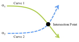
Figure 4: Reasoning about Intersection Points

Recall that we didn’t use $\alpha$ approximation at all. Since we already used $\alpha$ to prune candidate nodes in the first step, we do not use it again to prune potential curves or intersection points, since that may lead to incorrect results. In our experience, the lattice pruning step is more time-consuming (since we need to train a machine learning model for each expanded node), so it is more beneficial to use $\alpha$ in that step. We leave determining how to best integrate $\alpha$ into the learning algorithms as future work. Finally, the user can easily integrate domain knowledge, such as the distribution of item sizes, into the algorithm to further avoid computing and indexing intemediate intersection points.

Determining the Skyline: As we are determining the set of interesting intersection points, it is also easy to determine and maintain the skyline for each of these points. We simply walk up the list of candidate nodes at that point, sorted by cost, and keep all points that have not been dominated by previous points. (We keep track of the highest accuracy seen so far.)

Index Construction: Thus, our polydom indexing structure is effectively is a two-dimensional sorted array, where we store the skyline for different values of $n$. We have, first, a sorted array corresponding to the sizes of the input. Attached to each of these locations is an array containing the skyline of candidate curves.

For the intersection curve depicted in Figure 3, the index that we construct is depicted in Figure 5.

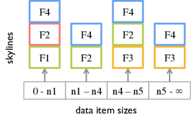
Figure 5: Poly-Dom Index for the feature sets in Figure 3

3.3 Online: Searching the Index

Given an instance of Problem 1 at real-time classification time, finding the optimal model is simple, and involves two steps. We describe these steps as it relates to Figure 5.

• We perform a binary search on the $n_{i}$ ranges, i.e., horizontally on the bottom most array, to identify the range within which the input item size $n_{0}$ lies.

• We then perform a binary search on the candidate nodes, i.e., vertically for the node identified in the previous step, to find the candidate node for which the cost is the largest cost is less than the target cost $c$. Note that we can perform binary search because this array is sorted in terms of cost. We then return the model corresponding to the given candidate node.

Thus, the complexity of searching for the optimal machine learning model is: $O(\log t_{int}+\log t_{cand})$: where $t_{int}$ is the number of interesting intersection points, while $t_{cand}$ is the number of candidate nodes on the skyline.

4 Greedy Solution

The second solution we propose, called Greedy, is a simple adaptation of the technique from Xu et al. [45]. Note that Xu et al.’s technique does not apply to generic machine learning algorithms, and only works with a specific class of SVMs; hence we had to adapt it to apply to all machine learning algorithms as a black box. Further, this algorithm (depicted in Algorithm 4 in the appendix) only works with a single size; multiple sizes are handed as described subsequently. For now, we assume that the following procedure is performed with the median size of items.

Expansion: Offline, the algorithm works as follows: for a range of values of $\lambda\in{\cal L}$, the algorithm does the following. For each $\lambda$, the algorithm considers adding one feature at a time to the current set of features that improves the most the function

gain = (increase in accuracy) — $\lambda\times$ (increase in cost)

This is done by considering adding one feature at a time, expanding the new set of features, and estimating its accuracy and cost. (The latter is a number rather than a polynomial — recall that the procedure works on a single size of item.) Once the best feature is added, the corresponding machine learning model for that set of features is recorded. This procedure is repeated until all the features are added, and then repeated for different $\lambda$s. The intuition here is that the $\lambda$ dictates the priority order of addition of features: a large $\lambda$ means a higher preference for cost, and a smaller $\lambda$ means a higher preference for accuracy. Overall, these sequences (one corresponding to every $\lambda\in{\cal L}$) correspond to a number of depth-first explorations of the lattice, as opposed to Poly-Dom, which explored the lattice in a breadth-first manner.

Indexing: We maintain two indexes, one which keeps track of the sequence of feature sets expanded for each $\lambda$, and one which keeps the skyline of accuracy vs. cost for the entire set of feature sets. The latter is sorted by cost. Notice that since we focus on a single size, for the latter index, we do not need to worry about cost functions, we simply use the cost values for that size.

Retrieval: Online, when an item is provided, the algorithm performs a binary search on the skyline, picks the desired feature set that would fit within the cost budget. Then, we look up the $\lambda$ corresponding to that model, and then add features starting from the first feature, computing one feature at a time, until the cost budget is exhausted for the given item. Note that we may end up at a point where we have evaluated more or less features than the feature set we started off with, because the item need not be of the same size as the item size used for offline indexing. Even if the size is different, since we have the entire sequence of expanded feature sets recorded for each $\lambda$, we can, when the size is larger, add a subset of features and still get to a feature set (and therefore a machine learning model) that is good, or when the size is smaller, add a superset of features (and therefore a model) and get to an even better model.

Comparison: This algorithm has some advantages compared to Poly-Dom:

• The number of models expanded is simply $|{\cal L}|\times|{\cal F}|^{2}$, unlike Poly-Dom, whose number of expanded models could grow exponentially in ${\cal F}$ in the worst case.

• Given the number of models stored is small (proportional to $|{\cal F}|\times|{\cal L}|$), the lookup can be simple and yet effective.

• The algorithm is any-time; for whatever reason if a feature evaluation cost is not as predicted, it can still terminate early with a good model, or terminate later with an even better model.

Greedy also has some disadvantages compared to Poly-Dom:

• It does not provide any guarantees of optimality.

• Often, Greedy returns models that are worse than Poly-Dom. Thus, in cases where accuracy is crucial, we need to use Poly-Dom.

• The $\lambda$ values we iterate over, i.e., ${\cal L}$, requires hand-tuning, and may not be easy to set. Our results are very sensitive to this cost function.

• Since Greedy uses a fixed size, for items that are of a very different size, it may not perform so well.

We will study the advantages and disadvantages in our experiments.

Special Cases: We now describe two special cases of Greedy that merit attention: we will consider these algorithms in our experiments as well.

• Greedy-Acc: This algorithm is simply Greedy where ${\cal L}=\{-\infty\}$; that is, this algorithm adds one at a time, the feature with the smallest cost at the median size.

• Greedy-Cost: This algorithm is simply Greedy where ${\cal L}=\{\infty\}$; that is, this algorithm adds one at a time, the feature that adds the most accuracy with no regard to cost.

Note that these two algorithms get rid of one of the disadvantages of Greedy, i.e., specifying a suitable ${\cal L}$.

5 Experiments

Online prediction depends on two separate phases—an offline phase to precompute machine learning models and data structures, and an online phase to make the most accurate prediction within a time budget. To this end, the goals of our evaluation are three-fold: First, we study how effectively the Poly-Dom and Greedy-based algorithms can prune the feature set lattice and thus reduce the number of models that need to be trained and indexed during offline pre-computation. Second, we study how these algorithms affect the latency and accuracy of the models that are retrieved online. Lastly, we verify the extent to which our anti-monotonicity assumption holds in real-world datasets.

To this end, we first run extensive simulations to understand the regimes when each algorithm performs well (Section 5.2). We then evaluate how our algorithms perform on a real-world image classification task (Section 5.3), and empirically study anti-monotonicity (Section B) and finally evaluate our algorithms on the real-wold classification task.

5.1 Experimental Setup

Metrics: We study multiple metrics in our experiments:

• Offline Feature Set Expansion (Metric 1): Here, we measure the number of feature sets “expanded” by our algorithms, which represents the amount of training required by our algorithm.

• Offline Index (Metric 2): Here, we measure the total size of the index necessary to look up the appropriate machine learning model given a new item and budget constraints.

• Online Index lookup time (Metric 3): Here, we measure the amount of time taken to consult the index.

• Online Accuracy (Metric 4): Here, we measure the accuracy of the algorithm on classifying items from the test set.

In the offline case, the reason why we study these two metrics (1 and 2) separately is because in practice we may be bottlenecked in some cases by the machine learning algorithm (i.e., the first metric is more important), and in some cases by how many machine learning models we can store on a parameter server (i.e., the second metric is more important). The reason behind studying the two metrics in the online case is similar.

Our Algorithms: We consider the following algorithms that we have either developed or adapted from prior work against each other:

• Poly-Dom: The optimal algorithm, which requires more storage and precomputation.

• Greedy: The algorithm adapted from Xu et al [45], which requires less storage and precomputation than Poly-Dom, but may expand a sub-optimal set of feature sets that result in lower accuracy when the item sizes change.

• Greedy-Acc: This algorithm involves a single sequence of Greedy (as opposed to multiple sequences) prioritizing for the features contributing most to accuracy.

• Greedy-Cost: This algorithm involves a single sequence of Greedy prioritizing for the features that have least cost.

Comparison Points: We developed variations of our algorithms to serve as baseline comparisons for the lattice exploration and indexing portions of an online prediction task:

• Lattice Exploration: Naive-Expand-All expands the complete feature set lattice.

• Indexing: While Poly-Dom only indexes points where the dominance relationship changes, Poly-Dom-Index-All indexes every intersection point between all pairs of candidate feature sets. Alternatively, Naive-Lookup does not create an index and instead scans all candidate feature sets online.

5.2 Synthetic Prediction Experiments

Our synthetic experiments explore how feature extraction costs, individual feature accuracies, interactions between feature accuracies, and item size variance affect our algorithms along each of our four metrics.

Synthetic Prediction: Our first setup uses a synthetic dataset whose item sizes vary between $1$ and $500$. To explore the impact of non-constant feature extraction costs, we use a training set whose sizes are all $1$, and vary the item sizes in the test dataset. For the feature sets, we vary four key parameters:

• Number of features $f_{i}$: We vary the number of features in our experiments from 1 to 15. The default value in our experiments is $12$.

• Feature extraction cost $c(f_{i},n)$: We randomly assign the cost function to ensure a high degree of intersection points. Each function is a polynomial of the form $c=a_{0}+a_{1}n+a_{2}n^{2}$ where the coefficients are picked as follows: $a_{0}\in[0,100]$, $a_{1}\in[0,\frac{100-a_{0}}{10}]$, $a_{2}\in[0,\frac{100-a_{0}-a_{1}}{4}]$. (The reason why typically $a_{0}<a_{1}<a_{2}$ is that $a_{1}$ is multiplied by $n$, while $a_{2}$ is multiplied by $n^{2}$.) We expect that typical cost functions are bounded by degree $n^{2}$ and found that this is consistent with the cost functions from the real-world task. Note that Poly-Dom is insensitive to the exact cost functions, only the intersection points.

• Single feature accuracy $a(\{f_{i}\})$: Each feature’s accuracy is sampled to be either helpful with probability $p$ or not helpful with probability $1-p$. If a feature is helpful, then its accuracy is sampled uniformly from within $[0.7,0.8]$ and within $[0.5,0.6]$ if it is not.

• Feature interactions $a(F_{i})$: We control how the accuracy of a feature set $F_{i}$ depends on the accuracy of its individual features using a parameterized combiner function:

  $$a_{k}(F_{i})=1-\Pi_{f_{j}\in F_{i}^{k}}(1-a(f_{j}))$$

  where $F_{i}^{k}$ are the top $k$ most accurate features in $F_{i}$. Thus when $k=1$, $F_{i}$’s accuracy is equal to its most accurate single feature. When $k=\infty$, $F_{i}$’s accuracy increases as more features are added to the set. We will explore $k=1$ and $\infty$ as two extremes of this combiner function. We denote the combiner function for a specific $k$ value as $cf_{k}$. Note that for any $k$, the accuracy values are indeed monotone. We will explore the ramifications of non-monotone functions in the real-world experiments.

We use the following parameters to specify a specific synthetic configuration: the number of features $n$, the parameter $p$, and $k$, the amount the features interact with each other. In each run, we use these parameters to generate the specific features, cost functions and accuracies that are used for all of the algorithms. Unless specified, the default value of $\alpha$ is $1.2$. For Greedy, the ${\cal L}=\{0,0.001,0.002,0.005,0.01,0.02,0.05,0.1,0.5,1,5,10\}$. Although we vary ${\cal L}$ over a large range, in practice the majority give rise to identical sequences because the dominating set of feature sets is fixed for a given item size (as assumed by Greedy).

Feature Set Expansions (Metric 1): We begin by comparing the number of models that Poly-Dom, Greedy and Naive-Expand-All train as a function of the combiner function and the number of features. This is simply the total number of unique feature For Poly-Dom and Naive-Expand-All, the number of feature sets is simply the number of nodes in the lattice that are expanded, while for Greedy this is simply the number of unique feature sets expanded.

Metric 1 Summary: On the synthetic dataset, for $cf_{1}$, the number of feature sets (i.e., lattice nodes) expanded by Poly-Dom’s lattice pruning phase for $\alpha=1.2$ is at least an order-of-magnitude (10$\times$) smaller than Naive-Expand-All, and is similar to Greedy.

While Poly-Dom with $\alpha=1$ expands similar to $\alpha=1.2$ for $cf_{1}$, it expands all features for $cf_{\infty}$. This is not surprising at all: $cf_{\infty}$ is designed to be a scenario where every intermediate feature set is “useful”, i.e., none of them get sandwiched between other feature sets.

In Figure 6 and Figure 6, we depict the number of feature sets expanded (in log scale) as a function of the number of features in the dataset along the $x$ axis, for $cf_{1}$ and $cf_{\infty}$ respectively. $p$ is set to $0.6$. The plots for other values are similar.

For both combiner functions, the total number of possible feature sets (depicted as Naive-Expand-All) scales very rapidly, as expected. On the other hand, the number of feature sets expanded by Poly-Dom for $\alpha=1.2$ grows at a much slower rate for both graphs, because Poly-Dom’s pruning rules allow it to “sandwich” a lot of potential feature sets and avoid expanding them. Consider first combiner function (i.e., Figure 6) For 10 features, Naive-Expand-All expands around 1000 feature sets, while Poly-Dom for $\alpha=1$ expands about 50, and $\alpha=1.2$ expands about 30. We find that the ability to effectively prune the lattice of feature sets depends quite a bit on the combiner function. While Poly-Dom with $\alpha=1.2$ continues to perform similarly. Poly-Dom $\alpha=1$ expands as much as Naive-Expand-All; this is not surprising given that all intermediate feature sets have accuracy values strictly greater than their immediate children. In comparison, Greedy expands about as many features as Poly-Dom with $\alpha=1.2$ but with a slower growth rate as can be seen from both $cf_{1}$ and $cf_{\infty}$; this is not surprising because in the worst case Greedy expands $|{\cal L}|\times|{\cal F}|^{2}$.

Indexing Size and Retrieval (Metric 2 and 3): Here, we measure the indexing and retrieval time of the Poly-Dom algorithms, which use a more complex indexing scheme than the Greedy algorithms.

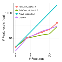
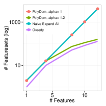
Figure 6: # of feature sets expanded vs # features for (a) $cf_{1}$ (b) $cf_{\infty}$

Metric 2 and 3 Summary: On the synthetic dataset, especially for larger numbers of features, the size of the Poly-Dom index is significantly smaller than the size of the Poly-Dom-Index-All index, and almost as small as the Naive-Lookup index. However, while Naive-Lookup has a smaller index size, Naive-Lookup’s retrieval time is much larger than Poly-Dom (for multiple values of $\alpha$), making it an unsuitable candidate.

In Figure 7 and Figure 7, we plot, for the two combiner functions the total size of the poly-dom index as the number of features is increased (for $\alpha=1.2,p=0.6$.) Consider the case when the number of features is $10$ for $cf_{1}$: here, Poly-Dom and Naive-Lookup’s index size are both less than 200, Poly-Dom-Index-All’s index size is at the 1000 mark, and rapidly increases to 6000 for 12 features, making it an unsuitable candidate for large numbers of features. The reason why Poly-Dom’s index size is smaller than Poly-Dom-Index-All is because Poly-Dom only indexes those points where the dominance relationship changes, while Poly-Dom-Index-All indexes all intersection points between candidate feature sets. Naive-Lookup, on the other hand, for both $cf_{1}$ and $cf_{\infty}$ only needs to record the set of candidate sets, and therefore grows slowly as well.

On the other hand, for retrieval time, depicted in Figures 8 and 8, we find that the Poly-Dom’s clever indexing scheme does much better than Naive-Lookup, since we have organized the feature sets in such a way that it is quick to retrieve the appropriate feature set given a cost budget On the other hand, Naive-Lookup does significantly worse than Poly-Dom, since it linearly scans all candidate feature sets to pick the best one — especially as the number of features increases.

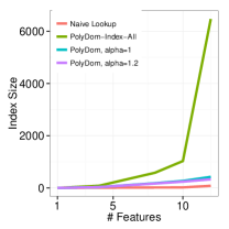
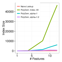
Figure 7: Index Size for (a) $cf_{1}$ (b) $cf_{\infty}$

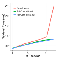
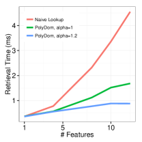
Figure 8: retrieval time for (a) $cf_{1}$ (b) $cf_{\infty}$

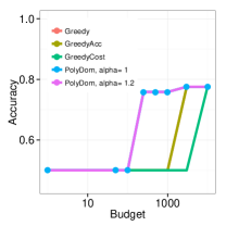
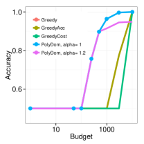
Figure 9: Accuracy as a function of budget (a) $cf_{1}$ (b) $cf_{\infty}$

Real-Time Accuracy (Metric 4): We now test the accuracy of the eventual model recommended by our algorithm.

Metric 4 Summary: On synthetic datasets, for $cf_{1}$ and $cf_{\infty}$, over a range of budgets, Poly-Dom (with both $\alpha=1$ or $1.3$), returns models with greater accuracies than Greedy and Greedy-Acc, which returns models with greater accuracies than Greedy-Cost. Often the accuracy difference (for certain budgets) between Poly-Dom and Greedy, or between Greedy and Greedy-Cost can be as high as 20%.

In figure 9 and 9, we plot the accuracy as a function of budget for Poly-Dom with $\alpha=1$ and $1.2$, and for Greedy, Greedy-Acc and Greedy-Cost. For space constraints, we fix the item size to $50$ and use $12$ features. $\alpha=1$ and $1.2$ is almost always better than Greedy. For instance, consider budget 1000 for $cf_{1}$ Poly-Dom with $\alpha=1\&1.2$ has an accuracy of about 80%, while Greedy, Greedy-Acc and Greedy-Cost all have an accuracy of about 50%; as another example, consider budget 1000 for $cf_{\infty}$, where Poly-Dom with $\alpha=1\&1.2$ has an accuracy of more than 90%, while Greedy, Greedy-Acc and Greedy-Cost all have accuracies of about 50%. In this particular case, this may be because Greedy, Greedy-Acc, and Greedy-Cost all explore small portions of the lattice and may get stuck in local optima. That said, apart from “glitches” in the mid-tier budget range, all algorithms achieve optimality for the large budgets, and are no better than random for the low budgets.

Further, as can be seen in the figure Greedy does better than Greedy-Cost, and similar to Greedy-Acc. We have in fact also seen other instances where Greedy does better than Greedy-Acc, and similar to Greedy-Cost. Often, the performance of Greedy is similar to one of Greedy-Acc or Greedy-Cost.

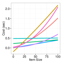
Figure 10: Varying size for (a) many features (b) one feature, but plotting quantiles

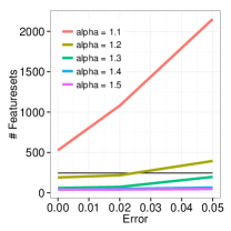
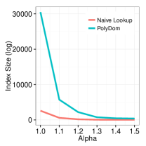
Figure 11: (a) Feature sets expanded (b) Index Size on varying $e$ (c) Index size on varying $\alpha$ (d) Accuracy vs. Budget

5.3 Real Dataset Experiments

Real Dataset: This subsection describes our experiments using a real image classification dataset [21]. The experiment is a multi-classification task to identify each image as one out of 15 possible scenes. There are 4485 labeled $250\times 250$ pixel images in the original dataset. To test the how our algorithms perform on varying image sizes, we rescale them to $65\times 65$, $125\times 125$ and $187\times 187$ pixel sizes. Thus in total, our dataset contains 17900 images. We use 8000 images as training and the rest as test images.

The task uses 13 image classification features (e.g., SIFT and GIST features) that vary significantly in cost and accuracy. In Figure 10, we plot the cost functions of eight representative features as a function of $n$, the item size, that we have learned using least squares curve fitting to the median cost at each training image size. As can be seen in the figure, there are some features whose cost functions are relatively flat (e.g., gist), while there are others that are increasing linearly (e.g., geo_map8$\times$8) and super-linearly (e.g., texton).

However, note that due to variance in feature evaluation time, we may have cases where the real evaluation cost does not exactly match the predicted or expected cost. In Figure 10, we depict the 10% and 90% percentile of the cost given the item size for a single feature. As can be seen in the figure, there is significant variance — especially on larger image sizes.

To compensate for this variation, we compute the cost functions using the worst-case extraction costs rather than the median. In this way, we ensure that the predicted models in the experiment are always within budget. Note that Greedy does not need to do this since it can seamlessly scale up/down the number of features evaluated as it traverses the sequence corresponding to a given $\lambda$. We did not consider this dynamic approach for the Poly-Dom algorithm.

The “black box” machine learning algorithm we use is a Linear classifier using stochastic gradient descent learning with hinge loss and L1 penalty. We first train the model over the training images for all possible combinations of features and cache the resulting models and cross-validation (i.e., estimated) accuracies. The rest of the experiments can look up the cached models rather than re-train the models for each execution.

For this dataset, our default values for $\alpha,e$ are $1.2,0$, respectively As we will see in the following, the impact of $e$ is small, even though our experiments described appendix B find that $e\geq 0$.

Feature Set Expansions (Metric 1):

Metric 1 Summary: On the real dataset, the number of feature sets expanded by Poly-Dom’s offline lattice pruning phase for $\alpha=1.2$ is $20\times$ smaller than Naive-Expand-All, with the order of magnitude increasing as $\alpha$ increases, and as $e$ decreases. Greedy expands a similar number of feature sets as Poly-Dom with $\alpha=1.2$.

In Figure 11, we depict the number of feature sets expanded (in log scale) as a function of the tolerance to non-monotonicity $e$ along the $x$ axis, for Poly-Dom with values of $\alpha=1.1,\ldots,1.5$, and for Greedy.

As can be seen in the figure, while the the total number of possible feature sets is close to $8200$ (which is what Naive-Expand-All would expand), the number of feature sets by Poly-Dom is always less than $400$ for $\alpha=1.2$ or greater, and is even smaller for larger $\alpha$s (the more relaxed variant induces fewer feature set expansions). Greedy (depicted as a flat black line) expands a similar number of feature sets as Poly-Dom with $\alpha=1.2$. On the other hand, for $\alpha=1.1$, more than 1/4th of the feature sets are expanded.

The number of feature sets expanded also increases as $e$ increases (assuming violations of monotonicity are more frequent leads to more feature set expansions).

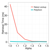
Figure 12: Retrieval time on varying (a) $e$ (b) $\alpha$

Indexing Size and Retrieval (Metric 2 and 3):

Metric 2 and 3 Summary: On the real dataset the size of the index for Poly-Dom is two orders of magnitude smaller than Poly-Dom-Index-All, while Naive-Lookup is one order of magnitude smaller than that. The index size increases as $e$ increases and decreases as $\alpha$ increases. However, the retrieval time for Poly-Dom is minuscule compared to the retrieval time for Naive-Lookup.

In Figure 11, we plot the total index size as the tolerance to non-monotonicity is increased (for $\alpha=1.3$.) As can be seen in the figure, the index size for Poly-Dom grows slowly as compared to Poly-Dom-Index-All, while Naive-Lookup grows even slower. Then, in Figure 11, we display the total index size that decreases rapidly as $\alpha$ is increased.

On the other hand, if we look at retrieval time, depicted in Figures 12 and 12 (on varying $e$ and on varying $\alpha$ respectively), we find that Naive-Lookup is much worse than Poly-Dom— Poly-Dom’s indexes lead to near-zero retrieval times, while Naive-Lookup’s retrieval time is significant, at least an order of magnitude larger. Overall, we find that as the number of candidate sets under consideration grows (i.e., as $\alpha$ decreases, or $e$ increases), we find that Poly-Dom does much better relative to Poly-Dom-Index-All in terms of space considerations, and does much better relative to Naive-Lookup in terms of time considerations. This is not surprising: the clever indexing scheme used by Poly-Dom pays richer dividends when the number of candidate sets is large.

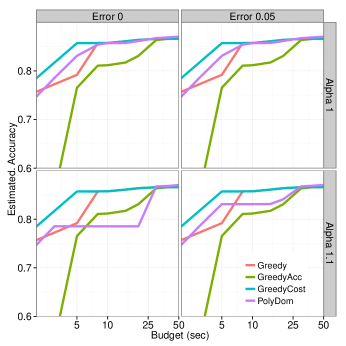
Figure 13: Estimated accuracy vs budget on varying $\alpha$ and $e$

Real-Time Accuracy (Metric 4):

Metric 4 Summary: On the real dataset, we find that while Poly-Dom still performs well compared to other algorithms for small $\alpha$, some Greedy-based algorithms are competitive, and in a few cases, somewhat surprisingly, better than Poly-Dom. All other things being fixed, the accuracy increases as the item size decreases, the budget increases, the $\alpha$ decreases, and $e$ increases.

In Figure 13, we plot the average estimated accuracy of the model retrieved given a budget for various values of $\alpha$ and $e$ for Poly-Dom, Greedy, Greedy-Acc, and Greedy-Cost across a range of image sizes. As can be seen in the figure, Poly-Dom dominates Greedy and Greedy-Acc apart from the case when $\alpha=1.1$. Even for $\alpha=1.1$, Poly-Dom dominates Greedy-Acc when $e=0.05$: here, we see that a higher $e$ leads to better performance, which we did not see in other cases.

Perhaps the most surprising aspect of this dataset is that Greedy-Cost dominates all the others overall. While the reader may be surprised that a Greedy-based algorithm can outperform Poly-Dom with $\alpha=1$, recall that the Greedy algorithms are any-time algorithms that can adapt to high variance in the feature evaluation cost, as opposed to Poly-Dom, which provisions for the worst-case and does not adapt to the variance. In future work, we plan to explore any-time variants of Poly-Dom, or hybrid variants of Poly-Dom with Greedy-based algorithms.

In Figure 11, we plot the estimated accuracy of the model retrieved as a function of the budget for various image sizes (across a number of images of the same size). As can be seen in the figure, the estimated accuracy is higher for the same size of image, as budget increases. Also, the estimated accuracy is higher for the same budget, as image size decreases (as the image size decreases, the same budget allows us to evaluate more features and use a more powerful model.)

6 Related Work

Despite its importance in applications, cost-sensitive real-time classification is not a particularly well-studied problem: typically, a feature selection algorithm [32] is used to identify a set of inexpensive features that are used with an inexpensive machine learning model (applied to all items, large or small), and there are no dynamic decisions enabling us to use a more expensive set of features if the input parameters allow it. This approach ends up giving us a classifier that is sub-optimal given the problem parameters. This approach has been used for real-time classification in a variety of scenarios, including: sensor-network processing [28, 8], object and people tracking [22, 36, 17], understanding gestures [29, 35], face recognition, speech understanding [3, 9], sound understanding [33, 39] scientific studies [16, 23], and medical analysis [31, 20]. All of these applications could benefit from the algorithms and indexing structures outlined in this paper.

Our techniques are designed using a wrapper-based approach [19] that is agnostic to the specific machine learning model, budget metric, and features to extract. For this reason, our approach can be applied in conjunction with a variety of machine learning classification or regression techniques, including SVMs [15], decision trees [27], linear or ridge regression [14], among others [12]. In addition, the budget can be defined in terms of systems resources, monetary metrics, time or a combination thereof.

There has been some work on adapting traditional algorithms to incorporate some notion of joint optimization with resource constraints, often motivated by a transition of these algorithms out of the research space and into industry. A few examples of this approach have been developed by the information retrieval and document ranking communities. In these papers the setup is typically described as an additive cascade of classifiers intermingled with pruning decisions. Wang et al notes that if these classifiers are independent the constrained selection problem is essentially the knapsack problem. In practice, members of an ensemble do not independently contribute to ensemble performance, posing a potentially exponential selection problem. For the ranking domain, Wang et al apply an algorithm that attempts to identify and remove redundant features [42], assemble a cascade of ranking and pruning functions [41], and develop a set of metrics to describe the efficienty-effectiveness tradeoff for these functions [40]. Other work focuses specifically on input-sensitive pruning aggresiveness [38] and early cascade termination strategies [6]. These approaches are similar in spirit to ours but tightly coupled to the IR domain. For example, redundant feature removal relies on knowledge of shared information between features (e.g., unigrams and bigrams), and the structure of the cascade (cycles of pruning and ranking) is particular to this particular problem. Further, these approaches are tuned to the ranking application, and do not directly apply to classification.

Xu’s classifier cascade work [7, 44, 43, 45] considers the problem of post-processing classifiers for cost sensitivity. Their approach results in similar benefits to our own (e.g., expensive features may be chosen first if the gains outweigh a combination of cheap features), but it is tailored to binary classification environments with low positive classification rate and does not dynamically factor in runtime input size. Others apply markov decision processes to navigate the exponential space of feature combinations [18], terminate feature computation once a test point surpasses a certain similarity to training points [24], or greedily order feature computation [25], but none of these formalize the notion of budget or input size into the runtime model, making it difficult to know whether high-cost high-reward features can be justified up front or if they should be forgone for an ensemble of lower-cost features. That said, our Greedy algorithm (along with its variants, Greedy-Acc and Greedy-Cost) are adapted from these prior papers [45, 25].

Our Poly-Dom algorithms are also related to prior work on the broad literature on frequent itemset mining [2], specifically [5, 26], that has a notion of a lattice of sets of items (or market baskets) that is explored incrementally. Further, portions of the lattice that are dominated are simply not explored. Our Poly-Dom algorithm is also related to skyline computation [37], since we are implicitly maintaining a skyline at all “interesting” item sizes where the skyline changes drastically.

Anytime algorithms are a concept from planning literature that describe algorithms which always produce some answer and continuously refine that answer give more time [10]. Our Greedy-family of algorithms are certainly anytime algorithms.

7 Conclusion and Future Work

In this paper, we designed machine-learning model-agnostic cost-sensitive prediction schemes. We developed two core approaches (coupled with indexing techniques), titled Poly-Dom and Greedy, representing two extremes in terms of how this cost-sensitive prediction wrapper can be architected. We found that Poly-Dom’s optimization schemes allow us to maintain optimality guarantees while ensuring significant performance gains on various parameters relative to Poly-Dom-Index-All, Naive-Lookup, and Naive-Expand-All, and many times Greedy, Greedy-Acc, and Greedy-Cost as well. We found that Greedy, along with the Greedy-Acc and Greedy-Cost variants enable “quick and dirty” solutions that are often close to optimal in many settings.

In our work, we’ve taken a purely black-box approach towards how features are extracted, the machine learning algorithms, and the structure of the datasets. In future work, we plan to investigate how knowledge about the model, or correlations between features can help us avoid expanding even more nodes in the lattice.

Furthermore, in this paper, we simply used the size of the image as a signal to indicate how long a feature would take to get evaluated: we found that this often leads to estimates with high variance (see Figure 10), due to which we had to provision for the worst-case instead of the average case. We plan to investigate the use of other “cheap” indicators of an item (like the size) that allow us to infer how much a feature evaluation would cost. Additionally, in this paper, our focus was on classifying a single point. If our goal was to evaluate an entire dataset within a time budget, to find the item with the highest likelihood of being in a special class, we would need very different techniques.

Appendix A Proof of Theorem 3.13

The following a proof of the poly-dom index construction algorithm described in Section 3.2.

Proof The proof follows a case analysis:

• Scenario 1: Curve 1 and 2 both on skyline and $\alpha_{1}>\alpha_{2}$

• Scenario 2: Curve 1 is not on the skyline while Curve 2 is

• Scenario 3: Curve 1 and 2 are both not on skyline

• Scenario 4: Curve 1 is on the skyline and Curve 2 is not, and $\alpha_{1}>\alpha_{2}$

The argument is that for Scenario 3 and 4, the skyline will not change: in scenario 3, Curve 1 and 2 will still not be on the skyline, while in Scenario 4, since Curve 1 gets even better, it will still be on the skyline, while Curve 2 will be dominated by Curve 1 and therefore will not be on the skyline.

On the other hand, for Scenario 1, Curve 1 will start dominating Curve 2, and so Curve 2 now is removed from the skyline. For Scenario 2, which is a little tricky, Curve 1, which is not on the skyline because of high cost, may move into the skyline if there is no other curve that dominates it (i.e., has lower cost and higher accuracy).

The other scenarios cannot happen:

• Other half of Scenario 1: Curve 1 and 2 are both on skyline, and $\alpha_{1}<\alpha_{2}$ cannot happen, because then Curve 2 would dominate Curve 1

• Other half of Scenario 4: Curve 1 is on the skyline while Curve 2 is not on the skyline and $\alpha_{1}<\alpha_{2}$ cannot happen since Curve 1 is dominated by Curve 2 $\square$

Appendix B Assumption Validation

In addition to the above performance metrics, we evaluated the sources of three types of variation that deviate from our assumptions.

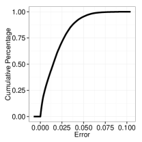
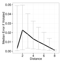
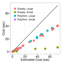
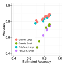
Figure 14: (a) CDF of anti-monotonicity (b) anti-monotonicity as a function of distance (c) Cost vs. Estimated Cost (d) Accuracy vs. Estimated Accuracy

Anti-monotonicity: First, we focus on the monotonicity assumption that we made on the real dataset, which we used to define the $e$ values used in the experiments. Although the monotonicity principle is anecdotally known to be true among machine learning practitioners, we were unable to find a reference for the practical evaluation of monotonicity on a real dataset. We view this as an additional contribution of our paper.

Figure 14 plots the cumulative distribution of the violations of monotonicity between pairs of ancestor-descendant feature sets in the lattice. Most of the violations are small: close to 95% of the violations are below an error of $5\%$, while all violations are within $7.5\%$. Thus, we believe the monotonicity principle is largely true, even on a real dataset. Note that we found fimor devations between the quality of the retrieved models as we decreased $e$ to $0$, so the assumptions that we made in the paper do not hurt us in a significant way.

Next, we would like to evaluate where in fact these violations of monotonicity exist in the lattice. Figure 14 evaluates the distribution of violations as a function of distance between feature set pairs. The black line is the median $e$ (with grey error bars) of all violations as a function of distance. As can be seen in the figure, the highest median $e$ as well as the largest variance is at distance $2$ and both quickly decrease to close to $0$ at $8$. This is a good sign: violations of monotonicity, if any, are local rather than global, with almost no violations that are between pairs of feature sets that are far away from each other. These results suggest that the Skyline algorithm is not likely to falsely prune a feature set early on due to a violation in monotonicity. Furthermore, a modest $e$ value can compensate for the majority of violations.

Estimated Versus Actual: Next, we compare the estimated cost and accuracies of the real-world model with the true values for large and small image sizes.

Figure 14 plots the estimated versusactual cost. We find that the cost function tends to over estimate the actual cost because the cost functions are trained on the worst, rather than average case. We chose this because if we did provision for the mean cost, the poly-dom index may return models whose true costs exceed the time budget. The costs for Greedy are similar, however because it ignores item size during the offline phase, it severely underestimates the cost of the small images, in contrast to Poly-Dom.

Figure 14 plots the estimated and true accuracy of the models retrieved. We find the the estimated accuracy is indeed linearly correlated with the true accuracy. However the model consistently overestimates the accuracy because the small images are downsampled, so the features are correspondingly less accurate. Overall, this suggests that optimizing for estimated accuracy is a reliable proxy for the quality of predictions at test time.

Appendix C Algorithm Pseudocode

Data: ${\cal F},n_{0},\alpha$

Result: ${\sf candidateSet}$

${\sf expandedNodes}=$ Expand-Enumerate $({\cal F},n_{0},\alpha)$;

${\sf toRemove}=\emptyset$;

for s, r $\in{\sf expandedNodes}$ do

       if s is dominated by r then

             add s to ${\sf toRemove}$;

            

      

${\sf candidateSet}={\sf expandedNodes}-{\sf toRemove}$;

Algorithm 1 Candidate-Set-Construction

Data: ${\cal F},n_{0},\alpha$

Result: ${\sf expandedNodes}$

${\sf activeTop}=\{{\cal F}\}$;

${\sf activeBottom}=\{\{\}\}$;

${\sf frontierTop}={\sf frontierBottom}={\sf expandedNodes}=\emptyset$;

while ${\sf activeTop}$ or ${\sf activeBottom}$ is non-empty do

       ${\sf activeTop2}={\sf activeBottom2}=\emptyset$;

       for s in ${\sf activeTop}$ do

             if s is not sandwiched between ${\sf frontierTop}$, ${\sf frontierBottom}$ AND has not been expanded then

                   expand $s$ and add to ${\sf expandedNodes}$;

                   add $s$’s children to ${\sf activeTop2}$;

                   add $s$ to ${\sf frontierTop}$;

                   remove $s$’s parents from ${\sf frontierTop}$;

                  

            remove $s$ from ${\sf activeTop}$;

            

      for s in ${\sf activeBottom}$ do

             if s is not sandwiched between ${\sf frontierTop}$, ${\sf frontierBottom}$ AND has not been expanded then

                   expand $s$ and add to ${\sf expandedNodes}$;

                   add $s$’s parents to ${\sf activeBottom2}$;

                   add $s$ to ${\sf frontierBottom}$;

                   remove $s$’s children from ${\sf frontierBottom}$;

                  

            remove $s$ from ${\sf activeBottom}$;

            

      ${\sf activeTop}={\sf activeTop2}$;

       ${\sf activeBottom}={\sf activeBottom2}$;

      

Algorithm 2 Expand-Enumerate

Data: ${\cal C},\alpha$

Result: ${\sf Poly-Dom}$

${\sf candCurves}=$ curves corresponding to ${\cal C}$;

${\sf sortedCurves}=$ sorted ${\sf candCurves}$ for $n<1$ on cost;

${\sf intPoints}=$ p.queue of int. pts. of neighboring curves;

while ${\sf IntPoints}$ is not empty do

       ${\sf singlePt}={\sf intPoints}.pop()$;

       update ${\sf sortedCurves}$ for ${\sf singlePt}$;

       ${\sf a,b}$ = curves that intersect at ${\sf singlePt}$;

       if ${\sf interesting(singlePt,sortedCurves)}$ then

             ${\sf ptsSoFar}.add({\sf singlePt}$);

            

      ${\sf intPoints}.add($new intersections of ${\sf a,b}$ with neighbors in ${\sf sortedCurves})$;

      

return ${\sf ptsSoFar}$;

Algorithm 3 PolyDomIntersections

Data: ${\cal F},n_{0}$

Result: ${\sf candidateSeq}$

for $\lambda\in{\cal L}$ do

       ${\sf curSet}=\emptyset$;

       ${\sf remSet}={\cal F}$;

       while ${\sf remSet}\neq\emptyset$ do

             add best feature $f\in{\sf remSet}$ to ${\sf curSet}$;

             ${\sf candidateSeq}(\lambda)$.append(model corresponding to ${\sf curSet}$);

             remove $f$ from ${\sf remSet}$;

            

      

return ${\sf candidateSeq}$;

Algorithm 4 Greedy Candidate-Sequences

References

- [1] Largest image. http://70gigapixel.cloudapp.net.
- [2] R. Agrawal, T. Imieliński, and A. Swami. Mining association rules between sets of items in large databases. In ACM SIGMOD Record, volume 22, pages 207–216. ACM, 1993.
- [3] J. N. Bailenson, E. D. Pontikakis, I. B. Mauss, J. J. Gross, M. E. Jabon, C. A. Hutcherson, C. Nass, and O. John. Real-time classification of evoked emotions using facial feature tracking and physiological responses. International journal of human-computer studies, 66(5):303–317, 2008.
- [4] J. Brutlag. Speed matters for google web search. http://googleresearch.blogspot.com/2009/06/speed-matters.html#!/2009/06/speed-matters.html. Published: 2009.
- [5] D. Burdick, M. Calimlim, and J. Gehrke. Mafia: A maximal frequent itemset algorithm for transactional databases. In Data Engineering, 2001. Proceedings. 17th International Conference on, pages 443–452. IEEE, 2001.
- [6] B. B. Cambazoglu, H. Zaragoza, O. Chapelle, J. Chen, C. Liao, Z. Zheng, and J. Degenhardt. Early exit optimizations for additive machine learned ranking systems. In Proceedings of the Third ACM International Conference on Web Search and Data Mining, WSDM ’10, pages 411–420, New York, NY, USA, 2010. ACM.
- [7] M. Chen, Z. E. Xu, K. Q. Weinberger, O. Chapelle, and D. Kedem. Classifier cascade for minimizing feature evaluation cost. In AISTATS, pages 218–226, 2012.
- [8] D. Comaniciu, V. Ramesh, and P. Meer. Real-time tracking of non-rigid objects using mean shift. In Computer Vision and Pattern Recognition, 2000. Proceedings. IEEE Conference on, volume 2, pages 142–149. IEEE, 2000.
- [9] B. Crawford, K. Miller, P. Shenoy, and R. Rao. Real-time classification of electromyographic signals for robotic control. In AAAI, volume 5, pages 523–528, 2005.
- [10] T. Dean and M. Boddy. Time-dependent planning. AAAI ’88, pages 49–54, 1988.
- [11] P. Domingos. A few useful things to know about machine learning. Communications of the ACM, 55(10):78–87, 2012.
- [12] R. O. Duda, P. E. Hart, and D. G. Stork. Pattern classification. John Wiley & Sons, 2012.
- [13] J. Hamilton. The cost of latency. http://perspectives.mvdirona.com/2009/10/31/TheCostOfLatency.aspx.
- [14] T. Hastie, R. Tibshirani, J. Friedman, T. Hastie, J. Friedman, and R. Tibshirani. The elements of statistical learning, volume 2. Springer, 2009.
- [15] M. A. Hearst, S. Dumais, E. Osman, J. Platt, and B. Scholkopf. Support vector machines. Intelligent Systems and their Applications, IEEE, 13(4):18–28, 1998.
- [16] Q. A. Holmes, D. R. Nuesch, and R. A. Shuchman. Textural analysis and real-time classification of sea-ice types using digital sar data. Geoscience and Remote Sensing, IEEE Transactions on, (2):113–120, 1984.
- [17] D. M. Karantonis, M. R. Narayanan, M. Mathie, N. H. Lovell, and B. G. Celler. Implementation of a real-time human movement classifier using a triaxial accelerometer for ambulatory monitoring. Information Technology in Biomedicine, IEEE Transactions on, 10(1):156–167, 2006.
- [18] S. Karayev, M. J. Fritz, and T. Darrell. Dynamic feature selection for classification on a budget. In International Conference on Machine Learning (ICML): Workshop on Prediction with Sequential Models, 2013.
- [19] R. Kohavi and G. H. John. Wrappers for feature subset selection. Artif. Intell., 97(1-2):273–324, Dec. 1997.
- [20] S. M. LaConte, S. J. Peltier, and X. P. Hu. Real-time fmri using brain-state classification. Human brain mapping, 28(10):1033–1044, 2007.
- [21] S. Lazebnik, C. Schmid, and J. Ponce. Beyond bags of features: Spatial pyramid matching for recognizing natural scene categories. In Computer Vision and Pattern Recognition, 2006 IEEE Computer Society Conference on, volume 2, pages 2169–2178. IEEE, 2006.
- [22] A. J. Lipton, H. Fujiyoshi, and R. S. Patil. Moving target classification and tracking from real-time video. In Applications of Computer Vision, 1998. WACV’98. Proceedings., Fourth IEEE Workshop on, pages 8–14. IEEE, 1998.
- [23] A. Mahabal, S. Djorgovski, R. Williams, A. Drake, C. Donalek, M. Graham, B. Moghaddam, M. Turmon, J. Jewell, A. Khosla, et al. Towards real-time classification of astronomical transients. arXiv preprint arXiv:0810.4527, 2008.
- [24] F. Nan, J. Wang, K. Trapeznikov, and V. Saligrama. Fast margin-based cost-sensitive classification. In Acoustics, Speech and Signal Processing (ICASSP), 2014 IEEE International Conference on, pages 2952–2956. IEEE, 2014.
- [25] P. Naula, A. Airola, T. Salakoski, and T. Pahikkala. Multi-label learning under feature extraction budgets. Pattern Recognition Letters, 40:56–65, 2014.
- [26] N. Pasquier, Y. Bastide, R. Taouil, and L. Lakhal. Efficient mining of association rules using closed itemset lattices. Information systems, 24(1):25–46, 1999.
- [27] J. R. Quinlan. Induction of decision trees. Machine learning, 1(1):81–106, 1986.
- [28] R. Rad and M. Jamzad. Real time classification and tracking of multiple vehicles in highways. Pattern Recognition Letters, 26(10):1597–1607, 2005.
- [29] M. Raptis, D. Kirovski, and H. Hoppe. Real-time classification of dance gestures from skeleton animation. In Proceedings of the 2011 ACM SIGGRAPH/Eurographics Symposium on Computer Animation, pages 147–156. ACM, 2011.
- [30] V. C. Raykar, B. Krishnapuram, and S. Yu. Designing efficient cascaded classifiers: tradeoff between accuracy and cost. In KDD, pages 853–860, 2010.
- [31] J. Rodriguez, A. Goni, and A. Illarramendi. Real-time classification of ecgs on a pda. Information Technology in Biomedicine, IEEE Transactions on, 9(1):23–34, 2005.
- [32] Y. Saeys, I. n. Inza, and P. Larrañaga. A review of feature selection techniques in bioinformatics. Bioinformatics, 23(19):2507–2517, Sept. 2007.
- [33] J. Saunders. Real-time discrimination of broadcast speech/music. In Acoustics, Speech, and Signal Processing, 1996. ICASSP-96 Vol 2. Conference Proceedings., 1996 IEEE International Conference on, volume 2, pages 993–996. IEEE, 1996.
- [34] E. Schurman and J. Brutlag. The user and business impact of server delays, additional bytes, and http chunking in web search. http://velocityconf.com/velocity2009/public/schedule/detail/8523, 2009.
- [35] J. Shotton, T. Sharp, A. Kipman, A. Fitzgibbon, M. Finocchio, A. Blake, M. Cook, and R. Moore. Real-time human pose recognition in parts from single depth images. Communications of the ACM, 56(1):116–124, 2013.
- [36] C. Stauffer and W. E. L. Grimson. Learning patterns of activity using real-time tracking. Pattern Analysis and Machine Intelligence, IEEE Transactions on, 22(8):747–757, 2000.
- [37] K.-L. Tan, P.-K. Eng, B. C. Ooi, et al. Efficient progressive skyline computation. In VLDB, volume 1, pages 301–310, 2001.
- [38] N. Tonellotto, C. Macdonald, and I. Ounis. Efficient and effective retrieval using selective pruning. In Proceedings of the Sixth ACM International Conference on Web Search and Data Mining, WSDM ’13, pages 63–72, New York, NY, USA, 2013. ACM.
- [39] G. Tzanetakis and P. Cook. Musical genre classification of audio signals. Speech and Audio Processing, IEEE transactions on, 10(5):293–302, 2002.
- [40] L. Wang, J. Lin, and D. Metzler. Learning to efficiently rank. In Proceedings of the 33rd International ACM SIGIR Conference on Research and Development in Information Retrieval, SIGIR ’10, pages 138–145, New York, NY, USA, 2010. ACM.
- [41] L. Wang, J. Lin, and D. Metzler. A cascade ranking model for efficient ranked retrieval. In Proceedings of the 34th International ACM SIGIR Conference on Research and Development in Information Retrieval, SIGIR ’11, pages 105–114, New York, NY, USA, 2011. ACM.
- [42] L. Wang, D. Metzler, and J. Lin. Ranking under temporal constraints. In Proceedings of the 19th ACM International Conference on Information and Knowledge Management, CIKM ’10, pages 79–88, New York, NY, USA, 2010. ACM.
- [43] Z. E. Xu, M. J. Kusner, G. Huang, and K. Q. Weinberger. Anytime representation learning. In ICML (3), pages 1076–1084, 2013.
- [44] Z. E. Xu, M. J. Kusner, K. Q. Weinberger, and M. Chen. Cost-sensitive tree of classifiers. In ICML (1), pages 133–141, 2013.
- [45] Z. E. Xu, K. Q. Weinberger, and O. Chapelle. The greedy miser: Learning under test-time budgets. In ICML, 2012.