Thin Tree Position

Abstract

We introduce a method for creating a special type of tree, a tree position, from a weighted graph. Leaves of the tree correspond to vertices of the original graph, and the tree edges contain information which can be used to partition these vertices. By repeatedly applying reducing operations to the tree position we arrive at a thin tree position, and we show that partitions arising from thin tree positions have especially nice properties. The algorithm is based the topological notion of thin position for knots and $3$–manifolds and builds on the previously defined idea of a Topological Intrinsic Lexicographic Order (TILO).

1 Introduction

A number of problems in machine learning, data mining and signal processing require that one find a partition of a graph with small boundary weight, but whose subsets have relatively large interior weights. These graphs may directly represent the given data (as in the case of social networks) or be derived from vector data via a heuristic such as $k$–nearest neighbors. In either case, these graphs often have millions of vertices, making a brute force search for efficient partitions infeasible.

In the present paper, we introduce an approach we call Thin Tree Position (TTP) for finding efficient partitions of graphs by carrying out a more targeted search, using intuition from three dimensional geometry/topology. This approach builds on the TILO/PRC (Topological Intrinsic Lexicographic Order / Pinch Ratio Clustering) algorithm introduced in [5] and [3], but improves on a number of deficiencies of this approach. The TILO/PRC approach consists of two steps: First, the TILO algorithm assigns a linear ordering to the vertices of the graph $G$ and then progressively improves this ordering with respect to a carefully chosen metric. Next, the PRC algorithm picks out consecutive blocks in the final TILO ordering that make up the partition.

Both TILO and TTP are algorithms that use ideas from low dimensional topology, specifically the concept of thin position of knots and $3$–manifolds [2, 9]. As such, these methods rely on the broad shape of the data set instead of its exact geometry. Carlsson has argued that algorithms of this type should perform well for certain problems and can give more information than existing methods [1]. We expect that TTP will be useful for clustering as well as other applications in topological data analysis.

The present approach addresses two major issues with TILO/PRC: First, the linear nature of TILO/PRC forces it to treat the subsets of the partition at the front and back of the TILO ordering differently from the subsets in the middle. As we describe in Section 2, the TTP algorithm replaces the linear ordering with a trivalent tree structure that allows all the subsets to be treated consistently. As we discuss in Section 3, this structure is a natural generalization of TILO orderings.

Second, the gradient-like TILO step of the TILO/PRC is relatively constrained. In order to make the search space reasonable, TILO only looks for ways to shift a single vertex at a time forward or backward in the ordering. Because TPT uses a tree structure, the equivalent step in TPT is able to move entire branches, which would be equivalent to allowing TILO to shift arbitrary subsets of consecutive vertices. However, as we describe in Section 4, this tree structure has a very simple reduction criterion analogous to that of TILO/PRC.

2 Thin position trees

Consider an undirected graph $G=(V,E)$ in which every edge $e\in E$ has two distinct vertices and every edge is assigned a positive real number $w(e)$ called its edge weight. In many cases, each edge weight will simply be 1. The weight of a subset of edges $F\subset E$ will be the sum of the weights of those edges, $w(F)=\sum_{f\in F}w(f)$. An edge is also specified by the two endpoints $f=(v_{i},v_{j})$ for $f\in E,v_{i},v_{j}\in V$. A short hand of the weight function is used for vertices

$$w(v_{i},v_{j})=\begin{cases}w(\ (v_{i},v_{j})\ )\ \text{ if }(v_{i},v_{j})\in E\\ 0\text{ if }(v_{i},v_{j})\notin E\\ \end{cases}$$

and for sets $A\subset V,B\subset V$,

$$w(A,B)=\sum_{v_{i}\in A,v_{j}\in B}w(v_{i},v_{j}).$$

Definition 1.

A $3$–Cayley tree [8] is a connected acyclic graph in which every non leaf vertex has degree of exactly three. We call the leaf vertices boundary vertices and the degree three vertices interior vertices.

A $3$–Cayley tree is also know as a boron tree [4] in which the interior vertices correspond to boron atoms and the boundary vertices correspond to hydrogen atoms. The number of interior vertices of a $3$–Cayley tree is always two less than the number of boundary vertices; this can be proved, for example, using an inductive argument, or from the fact that the Euler characteristic of a tree is one.

We will use $3$–Cayley trees to study general graphs as follows:

Definition 2.

Given a finite graph $G$, possibly with weighted edges, a tree position for $G$ is a pair $(C,\phi)$ where $C$ is a $3$–Cayley tree and $\phi$ is a one to one map from the vertices of $G$ onto the boundary vertices of $C$.

Figure 1 presents example tree positions $(C,\phi)$ and $(C^{\prime},\phi^{\prime})$ for the graph at the top of the figure. The outlined circles represent interior vertices, while the filled in circles are boundary vertices of a tree position. In this figure, the relative positions of the vertices of the graph are maintained in displaying the boundary vertices of the tree positions.

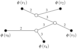
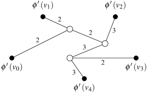
Figure 1: Graph $G$ with tree positions $(C,\phi)$ and $(C^{\prime},\phi^{\prime})$.

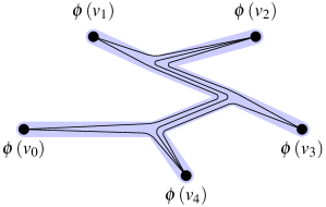
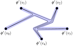
Figure 2: Edges of $G$ drawn through tree positions $(C,\phi)$ and $(C^{\prime},\phi^{\prime})$.

Given a tree position $(C,\phi)$ for a graph $G$, let $v,w$ be vertices of $G$ spanned by an edge $e$. Because $C$ is a tree, there is a unique simple path in $C$ from $\phi(v)$ to $\phi(w)$. We say that the edge $e$ passes through each of these edges of $C$. In other words, if $f$ is an edge of $C$ then for any topological map from the realization of $G$ to the realization of $C$, as in the picture of Figure 2, the image of $e$ would be forced to intersect $f$. For an edge $f$ of $C$, let $R(f)$ be the set of edges of $G$ that pass through $f$.

Definition 3.

Given a subtree $T$ of a tree position $(C,\phi)$ of $G=(V,E)$, the set of vertices of $V$ that are the image of the boundary vertices in $T$ is $\phi^{-1}\!\left({T}\right)=\left\{v\in V\ |\ \phi\left({v}\right)\in T\right\}$.

Definition 4.

Let $f$ and $g$ be two distinct edges of a tree position $(C,\phi)$. Two subtrees of $C$ are defined by cutting the edge $f$. The subtree containing $g$ is denoted $T\left({f},{g}\right)$, and the subtree not containing $g$ is denoted $\overline{T}\left({f},{g}\right)$.

Note that one endpoint of $f$ is in $T\left({f},{g}\right)$ and the other is in $\overline{T}\left({f},{g}\right)$. Thus cutting an edge $f$ of a tree position $(C,\phi)$ divides the vertices of $G$ into two disjoint sets: $\phi^{-1}\!\left({T\left({f},{g}\right)}\right)$ and $\phi^{-1}\!\left({\overline{T}\left({f},{g}\right)}\right)$.

Definition 5.

Given a tree position $(C,\phi)$ for a graph $G$, the width $b(f)$ of an edge $f$ in $C$ is the sum of the weights of the edges of $G$ that pass through $f$:

$$b(f)=w\left(R(f)\right)=w\left(\phi^{-1}\!\left({T\left({f},{g}\right)}\right),\phi^{-1}\!\left({\overline{T}\left({f},{g}\right)}\right)\right)$$

or for some edge $g$ of $C$ with $g\neq f$.

Note that we indicate the width of $f$ by $b(f)$ rather than $w(f)$ because it is equal to the area of the boundary of the subset of $G$ defined by the boundary vertices in either of the subtrees of $C$ defined by removing $f$. This notation is also in line with the notation in [5]. A notion of width for a tree position, analogous to the width of a TILO ordering, is created by placing the widths of all of the tree edges into a multiset and sorting in nonincreasing order. Tree widths can then be compared by a lexicographic ordering of the widths. In Figure 1 the edges of graph $G$ have weight one and the edges of the tree positions are denoted with their width. The width of $(C,\phi)$ is (3,3,3,3,2,2,2) and the width of $(C^{\prime},\phi^{\prime})$ is (3,3,3,2,2,2,2). Since the width of $(C^{\prime},\phi^{\prime})$ is less than the width of $(C,\phi)$, we say that tree position $(C^{\prime},\phi^{\prime})$ is thinner than tree position $(C,\phi)$. As with linear TILO, we would like to find tree positions whose widths are as low as possible. To do this, a branch shift operation that is analogous to the TILO shift is defined. A branch shift is described by two equivalent operations: first an edit operation of removing and reattaching a vertex (see Figure 3), and second a cyclic shifting of edges (see Figure 4).

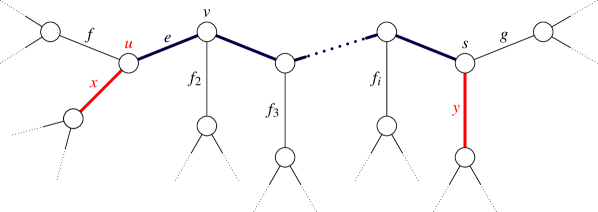
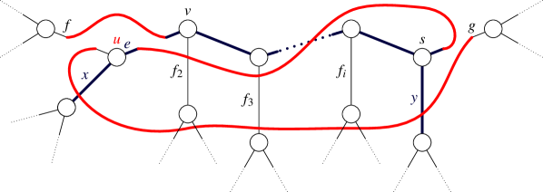
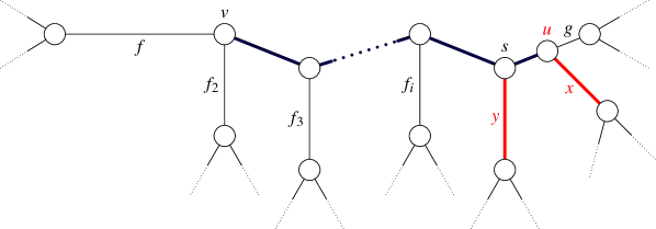
Figure 3: Branch shift of $x$ to $y$ as an edit operation

Given a $3$–Cayley tree $C$, let $x$ and $y$ be edges of $C$ that do not share a common endpoint. Since $C$ is a tree, there is a unique simple path from $x$ to $y$. Let vertex $u$ be the endpoint of $x$ that is shared with the first edge of the path, $e$. Let edge $f$ be other edge sharing vertex $u$. Removing vertex $u$ from $C$ is the operation of disconnecting edge $e$ from vertex $v$ (the other endpoint of $e$), disconnecting edge $f$ from vertex $u$, and attaching the free end of $f$ to vertex $v$. Let vertex $s$ be the common endpoint of $y$ and the last edge of the path. Let edge $g$ be adjacent to $y$ and the last edge of the path. Adding vertex $u$ to $C$ is the operation of disconnecting edge $g$ from from vertex $s$, attaching the free end of edge $e$ to vertex $s$, and attaching the free end of edge $g$ to vertex $u$. See Figure 3 for an example in which the original tree position is at the top, the middle is the tree position after modifying the edges but not moving any vertices in the display, and the bottom is the same tree position but with vertex $u$ moved in the display.

An alternative view of a branch shift operation is that of a cyclic shift of the edges adjacent to the path from $x$ to $y$. In this view, $x$, $y$, and all of the non-path edges sharing a vertex in the interior of the path are disconnected. Edge $x$ is reattached at edge $y$’s old location. The rest of the edges are reattached one vertex over in the direction of $x$. See Figure 4 for an example.

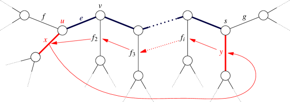
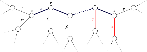
Figure 4: Branch shift of $x$ to $y$ as a cyclic shift of branches

The difference between viewing the branch shift as a cyclic shift of edges and the edit operation is just a relabelling of edges and internal nodes. The cyclic shift of edges will be used when making a connection to shift operations on TILO linear orderings. A typical software implementation will use the edit operation. Applying the branch shift move on $C$ creates the new tree $C^{\prime}$ and is described as shifting $x$ to $y$. Note that shifting $y$ to $x$ produces a different tree than shifting $x$ to $y$.

If we perform a branch shift on a $3$–Cayley tree $C$, the boundary vertices of $C$ are not touched. There is thus a canonical map from the boundary vertices of $C$ to the boundary vertices of $C^{\prime}$. If $(C,\phi)$ is a tree position for a graph $G$ then composing $\phi$ with this canonical map defines a one to one map $\phi^{\prime}$ from the vertices of $G$ to the boundary vertices of $C^{\prime}$, which in turn defines a new tree position for $G$. In this paper, $C$ and $C^{\prime}$ will share the same set of boundary vertices and the canonical map is just the identity map, $\phi$= $\phi^{\prime}$.

Definition 6.

The tree position $(C^{\prime},\phi)$ is a branch shift of $(C,\phi)$ when $C^{\prime}$ is a branch shift of $C$.

The new tree position defined by a branch shift has its own width, which may be higher or lower than the original.

Definition 7.

A tree position $(C,\phi)$ is weakly reducible if there is a branch shift that produces a new tree position with strictly lower width. Otherwise, $(C,\phi)$ is strongly irreducible or a thin tree position.

3 Comparing TILO tree position orderings to TILO linear orderings

Initially, the idea of tree position may appear to be completely different from the linear orderings used in the original TILO algorithm. However, as we will see in this section, it is in fact a very natural generalization.

The TILO algorithm as described in [5] begins with a linear ordering of the vertex set $V$, i.e. a one to one function from $V$ onto the set $[0,N-1]=\{0,1,\ldots,N-1\}$, where $N$ is the number of vertices in $V$. We will call this function a TILO ordering. A TILO ordering of $V$ defines a sequence of subsets $A_{i}=\{v\in V\ |\ o(v)\leq i\}$. This, in turn, defines a sequence of boundary widths $b_{i}=w(A_{i},\overline{A}_{i})$ where $\overline{A}_{i}=\{v\in V|v\notin A_{i}\}$ is the complement of $A_{i}$. Given a TILO ordering $o:V\rightarrow[0,N-1]$, we say that a second TILO ordering $o^{\prime}$ is the result of a shift on $o$ from $a$ to $b$ if $o^{\prime}$ of the composition of $o$ with a cyclic permutation of the block $[a,b]$ of consecutive numbers in $[0,N-1]$ that sends $a$ to position $b$. For example, for $N=8$, a shift of $2$ to $5$ takes the sequence $0,1,2,3,4,5,6,7$ to $0,1,3,4,5,2,6,7$. The shift from $5$ to $2$ takes the initial sequence to $0,1,5,2,3,4,6,7$. The width of a TILO ordering is the multiset of widths $b_{i}$ sorted in nonincreasing order. Lexicographic order is used to compare widths.

Definition 8.

A TILO linear ordering $o$ is called weakly reducible if it satisfies the reduction criteria in Lemma 1. A TILO linear ordering is called strongly irreducible if it is not weakly reducible.

By definition, a weakly reducible ordering admits a shift that decreases its width. The TILO algorithm performs the series of shifts determined by Lemma 1 that reduce the width until it finds a strongly irreducible ordering. (Because there are a finite number of orderings, at least one must be strongly irreducible.) To present Lemma 1, we first need to define slope $s_{i,k}$ with respect to order $o$ is as the sum of the edges from vertex $v_{o(k)}$ to other vertices in $\overline{A}_{i}$ minus the sum of edges from $v_{o(k)}$ to other vertices in $A_{i}$:

$$s_{i,k}=w\left(v_{o(k)},\overline{A}_{i}\setminus\{v_{o(k)}\}\right)-w\left(v_{o(k)},A_{i}\setminus\{v_{o(k)}\}\right)$$ (1)

where $\setminus$ means set difference. The adjacency $a_{i,j}$ with respect to order $o$ is the edge weight between the $i$-th and $j$-th vertices of order $o$: $a_{i,j}=w(v_{o(i)},v_{o(j)})$. The following lemma is a slight rewording of [5, Lemma 3] for the case of shifting a vertex earlier in a ordering with a vertex later in the ordering.

Lemma 1.

A TILO linear ordering $o$ is weakly reducible if for some $i$ and $k$ such that $k<i$ the following conditions hold:

$$s_{i,k}>0,$$

$$b_{t-1}\leq b_{t}\ \text{ for all }\ k<t\leq i,\text{ and}$$

$$s_{i,k}-s_{i,i+1}-2a_{k,i+1}>0.$$

In this case, shifting $k$ to $i$ reduces the width of $o$.

The analogous result for when $k>i$ also holds but is not needed for this paper.

To make a connection between a linear ordering and a path view of a tree ordering, the following structures are defined. Recall that a partition $\mathcal{P}$ of a set $A$ is a collection of pairwise disjoint subsets $\mathcal{P}=\{P_{0},\ldots,P_{k}\}$ of $A$ whose union is $A$. In other words, each element of $A$ is in exactly one subset $P_{j}$.

Definition 9.

Given a graph $G=(V,E)$ and a partition $\mathcal{P}$ of $V$, the quotient graph $Q=Q(G,\mathcal{P})$ is a weighted graph whose vertices correspond to elements $P_{j}$ of $\mathcal{P}$ and whose edges are defined as follows: if $v_{s}\in P_{i}$, $v_{t}\in P_{j}$, $i\neq j$, and $(s,t)\in E$ then there is an edge $(i,j)$ in $Q$ with weight $w(P_{i},P_{j})$.

Note that the quotient graph only accounts for edges that go between different sets in the partition and ignores edges between vertices that are in the same subset $P_{j}$. The quotient graph corresponds to a coarsening of the original graph in multilevel graph algorithms [6, 7].

A tree position $(C,\phi)$ for a graph $G$ can be used to define a number of different partitions of $G$. This paper is interested in a partitioning related to the branch shift operation with the following definition.

Definition 10.

Given a tree position $(C,\phi)$ for a graph $G$ and any pair of nonadjacent edges $x$ and $y$, we can construct a partition of the vertices of $G$ using the following approach. Denote the edges in the unique simple path from $x$ to $y$ as $p_{t}$ with $t=1$ for the edge adjacent to $x$ and $t=i$ for the edge adjacent to $y$. Label the edges sharing a common vertex with adjacent path edge pairs as follows: $p_{0}$ for pair $x$ and $p_{1}$, $p_{i+1}$ for pair $y$ and $p_{i}$, and $f_{t}$ for pair $p_{t-1}$ and $p_{t}$ with $2\leq t\leq i$. See Figure 6 for an example. Define the sets $P_{t}$ as

$$P_{0} =\phi^{-1}\!\left({\overline{T}\left({p_{0}},{y}\right)}\right),$$

$$P_{1} =\phi^{-1}\!\left({\overline{T}\left({x},{y}\right)}\right),$$

$$P_{t} =\phi^{-1}\!\left({\overline{T}\left({f_{t}},{y}\right)}\right)\ \text{ for }2\leq t\leq i,$$

$$P_{i+1} =\phi^{-1}\!\left({\overline{T}\left({y},{x}\right)}\right),$$

$$P_{i+2} =\phi^{-1}\!\left({\overline{T}\left({p_{i+1}},{y}\right)}\right).$$

We will call the quotient graph created using the partition $\mathcal{P}=\left\{P_{0},\dots,P_{i+2}\right\}$ the branch shift quotient graph of $G$ induced from $x$, $y$, and $(C,\phi)$.

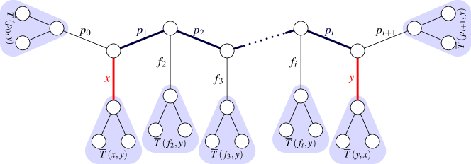
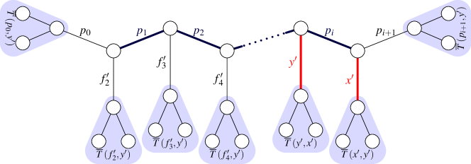
Figure 5: Before cyclic branch shift of $x$ to $y$

Figure 6: After cyclic branch shift of $x$ to $y$

The partitions $P_{j}$ of a branch shift quotient graph are disjoint. The only vertices not in the union of subtrees cut from $C$ are the vertices along the path from $x$ to $y$, which must be interior vertices. Hence all of the boundary vertices are covered by the subtrees and the mapping back to $G$ covers all of the vertices of $G$. Thus $\mathcal{P}$ is indeed a partition of $V$.

The smallest number of partitions in a branch shift quotient graph of G induced from $x$, $y$, and $(C,\phi)$ is four. This occurs when the path from $x$ to $y$ is just a single edge. The largest possible number of partitions in a branch shift quotient graph is $|V|$, the number of vertices in $G$. This occurs when the path from $x$ to $y$ contains every interior vertex of $C$. Each partition is then a singleton set.

TILO uses a linear ordering of vertices. A natural ordering of the vertices of $Q$ is to use an identity map. That is, if $u_{j}$ is the vertex of $Q$ corresponding to subset $P_{j}$ then it is in the $j$th position of the linear order. We demonstrate a connection between this TILO ordering and the tree position with a series of Lemmas.

Lemma 2.

Given a branch shift quotient graph $Q$ induced from edges $x$, $y$, and tree position $(C,\phi)$, the $t$-th width $b_{Q}(t)$ using the identity map ordering on $Q$ is equal to $b(p_{t})$, the width of edge $p_{t}$ on the tree position $(C,\phi)$ where path edges $p_{t}$ are defined in Definition 10.

Proof.

The $t$-th width using the identity map linear ordering of vertices is the sum of edge weights for edges $(j,k)\in Q$ such that $v_{j}$ is in set $\{v_{0},\ldots,v_{t}\}$ and $v_{k}$ is in set $\{v_{t+1},\ldots,v_{i+2}\}$. Since edge weight $(j,k)$ is defined as weight $w(P_{j},P_{k})$, this becomes

$$b_{Q}(t)=w\left(\bigcup_{0\leq j\leq t}P_{j},\bigcup_{t<k\leq i+2}P_{k}\right).$$

Recall that the boundary at an edge in $C$ can be defined in terms of all the edges of $G$ that pass through it, $b(p_{t})=\sum_{g\in R(p_{t})}w(g)$, or in terms of the edges between the sets of vertex images of the subtrees created by cutting at $p_{t}$,

$$b(p_{t})=w\left(\phi^{-1}\!\left({T\left({p_{t}},{p_{0}}\right)}\right),\phi^{-1}\!\left({\overline{T}\left({p_{t}},{p_{0}}\right)}\right)\right).$$

Edge $p_{t}$ is not contained in any subtree used to define the partitions in Definition 10 therefore each subtree (and corresponding partition) must be completely on one side of the cut of edge $p_{t}$. Thus

$$P_{j} \subseteq\phi^{-1}\!\left({T\left({p_{t}},{p_{0}}\right)}\right)\ \text{ for }\ 0\leq j\leq t\ \text{and}$$

$$P_{k} \subseteq\phi^{-1}\!\left({\overline{T}\left({p_{t}},{p_{0}}\right)}\right)\ \text{ for }\ t<k\leq i+2.$$

Since subsets $P_{j}$, $P_{k}$ form a partition and

$$\phi^{-1}\!\left({T\left({p_{t}},{p_{0}}\right)}\right)\ \bigcap\ \phi^{-1}\!\left({\overline{T}\left({p_{t}},{p_{0}}\right)}\right)=\emptyset$$

then

$$\phi^{-1}\!\left({T\left({p_{t}},{p_{0}}\right)}\right)\subseteq\bigcup_{0\leq j\leq t}P_{j}\quad\text{ and }\quad\phi^{-1}\!\left({\overline{T}\left({p_{t}},{p_{0}}\right)}\right)\subseteq\bigcup_{t<k\leq i+2}P_{k}.$$

With the two pair of sets being equal, the weights are also equal:

$$b_{Q}(t) =w(\bigcup_{0\leq j\leq t}P_{j},\bigcup_{t<k<=i+2}P_{k})$$

$$=w(\phi^{-1}\!\left({T\left({p_{t}},{p_{0}}\right)}\right),\phi^{-1}\!\left({\overline{T}\left({p_{t}},{p_{0}}\right)}\right))$$

$$=b(p_{t}).$$

∎

A branch shift on tree position $(C,\phi)$ creates a new tree position $(C^{\prime},\phi)$ for $G$. Let the branch shift be the shifting of edge $x$ to edge $y$ for any pair $x$ and $y$ of nonadjacent edges of $C$. Let $Q$ be the branch shift quotient graph of $G$ induced from $x$, $y$, and $(C,\phi)$. Using the notation from Definition 10, the before and after views of a branch shift are presented in Figures 6 and 6. Note that the edges $p_{0}$ to $p_{i+2}$ are not modified nor are the subtrees opposite the cut of edges $x^{\prime}$, $y^{\prime}$, $f_{2}^{\prime}$ to $f_{i}^{\prime}$. Let $Q^{\prime}$ be the branch shift quotient graph of $G$ induced from $f_{2}^{\prime}$, $x^{\prime}$, and $(C^{\prime},\phi)$.

Lemma 3.

The branch shift quotient graph $Q^{\prime}$ defined above is equal to the original branch shift quotient graph $Q$.

Proof.

The each $P_{j}$ of the partition used by the original branch shift quotient graph is defined in Definition 10 using the subtree from the far side cut of an edge adjacent to, but not on, the path between $x$ and $y$. The branch shift operation cuts these edges and then reattaches them to vertices on the path between $x$ and $y$. This operation does not touch the subtree on the far side cut of the edge. Thus the subsets $P_{k}^{\prime}$ used by $Q^{\prime}$ are just a relabelling of original subsets; explicitly, $P_{0}^{\prime}=P_{0}$, $P_{i+2}^{\prime}=P_{i+2}$, $P_{i+1}^{\prime}=P_{1}$, and $P_{t}^{\prime}=P_{t+1}$ for $1\leq t\leq i$. Therefore, the partition defined after the branch shift is the same as the partition before the shift and hence the quotient graphs are equal. ∎

Since the quotient graphs are equal, i.e. $Q^{\prime}=Q$, we can compare the linear TILO orderings on $Q$ defined by the tree positions $(C,\phi)$ and $(C^{\prime},\phi)$.

Lemma 4.

The TILO ordering on $Q$ defined by $(C^{\prime},\phi)$ is the result of starting with the ordering defined by $(C,\phi)$ and cyclicly shifting the vertex at position $1$ to position $i+1$.

Proof.

Let $u_{j}$ and $u_{j}^{\prime}$ be the vertices of $Q$ and $Q^{\prime}$, respectively. As noted in the proof of Lemma 3, the subsets $P_{k}^{\prime}$ used by $Q^{\prime}$ are relabelling of the subsets $P_{j}$ used by $Q$. This results in the following relabelling of vertices: $u_{0}^{\prime}=u_{0}$, $u_{i+2}^{\prime}=u_{i+2}$, $u_{i+1}^{\prime}=u_{1}$, and $u_{t}^{\prime}=u_{t+1}$ for $1\leq t\leq i$. The identity map linear ordering of $Q^{\prime}$ is $(u_{0}^{\prime},u_{1}^{\prime},u_{2}^{\prime},\ldots,u_{i}^{\prime},u_{i+1}^{\prime},u_{i+2}^{\prime})$. Substituting $Q$ vertices into this sequence yields the vertex order $(u_{0},u_{2},u_{3},\ldots,u_{i},u_{i+1},u_{1},u_{i+2})$. This is precisely the result of applying a cyclic shift of vertex $u_{1}$ to vertex $u_{i+1}$ of the identity map linear ordering of $Q$. ∎

Corollary 5.

A tree position $(C,\phi)$ of a graph $G$ is weakly reducible if there is a pair of edges in $C$ such that the TILO ordering of the induced branch shift quotient graph $Q$ of $G$ is weakly reducible.

Proof.

Note that if $(C^{\prime},\phi)$ is the result of a branch shift of edge $x$ to edge $y$ on a tree position $(C,\phi)$ then the width of the edges that are not along the path from $x$ to $y$ do not change. The only widths that change are along the path from $x$ to $y$, and by Lemma 4, the way they change is determined by the changes to the induced orderings of the quotient graph.

Assume there is a path in which the induced ordering on the quotient graph is weakly reducible, i.e. admits a shift that reduces its width. This TILO shift determines a branch shift of the tree position. Under this branch shift, the widths of the edges outside the path do not change. Along the path, some of the widths may increase, but at least one width strictly decreases and no width increases to a value greater than or equal to the highest width that strictly decreases. The same condition is true of the overall multiset of widths of the tree position, so the width of the resulting tree position is strictly less than the original width.

∎

4 Reduction criteria

Corollary 5 suggests a straightforward way to find strongly irreducible tree positions of graphs: take all pairs of edges, form the induced branch shift quotient graph, look for valid TILO shifts, and apply the corresponding branch shifts on the tree position. Repeat this process until there are no valid TILO shifts, and then perform a more comprehensive check to ensure that the tree position is indeed strongly irreducible. However, such an approach involves a great deal of redundant computation. In particular, if two paths overlap along a stretch of edges, then there will be TILO moves in the two different quotients that correspond to the same branch shifts. In a naive implementation these will be checked multiple times. We therefore define criteria for weak reducibility of a tree position that are determined by the quotient graphs but do not require explicitly computing them.

Definition 11.

Given a tree position $(C,\phi)$ and a pair of edges $e,g$ of $C$, define the adjacency weight

$$a(e,g)=w\left(R(e)\cap R(g)\right)=w\left(\phi^{-1}\!\left({\overline{T}\left({e},{g}\right)}\right),\phi^{-1}\!\left({\overline{T}\left({g},{e}\right)}\right)\right)$$

to be the sum of the weights of the edges of $G$ that pass through both $e$ and $g$ or equivalently the sum of the weights of edges of $G$ between boundary vertices in $\overline{T}\left({e},{g}\right)$ and boundary vertices in $\overline{T}\left({g},{e}\right)$.

Define the slope

$$s(e,g) =w\left(R(g)\setminus R(e)\right)-w\left(R(e)\cap R(g)\right)$$

$$=w\left(\phi^{-1}\!\left({T\left({g},{e}\right)}\right)\setminus\phi^{-1}\!\left({\overline{T}\left({e},{g}\right)}\right),\overline{T}\left({g},{e}\right)\right)-w\left(\phi^{-1}\!\left({\overline{T}\left({e},{g}\right)}\right),\phi^{-1}\!\left({\overline{T}\left({g},{e}\right)}\right)\right)$$

to be the sum of the weights of the edges of $G$ that pass through $g$ but not through $e$ minus the sum of the weights of edges of $G$ that pass through both edges. The slope $s(e,g)$ is the amount that the width of edge $e$ changes if edge $g$ is disconnected from the tree and reattached on the far side of $e$.

From the definitions, it follows that

$$a(e,g)+s(e,g)=w(R(g)\setminus R(e)).$$

From basic set theory,

$$R(g)=(R(g)\cap R(e))\cup(R(g)\setminus R(e))$$

where the sets $R(g)\cap R(e)$ and $R(g)\setminus R(e)$ are disjoint. Thus we have $b(g)=a(e,g)+a(e,g)+s(e,g)$. Rearranging this gives us an alternate way to calculate $s(e,g)$:

Lemma 6.

The slope $s(e,g)$ can also be calculated by the equation

$$s(e,g)=b(g)-2a(e,g).$$

If we think of the vertices $u_{e}$ and $u_{g}$ in a quotient graph that correspond to the subtrees $\overline{T}\left({e},{g}\right)$ and $\overline{T}\left({g},{e}\right)$, respectively, then the adjacency weight $a(e,g)$ is the weight of edge $(e,g)$ of the quotient graph. If $u_{e}$ and $u_{g}$ are vertices in a branch shift quotient graph then the slope $s(e,g)$ is $\pm s_{e,g}$, the slope (as defined in [5]) of a linear ordering of the vertices of the induced quotient graph. In particular, we have the following:

Lemma 7.

Given $Q$, a branch shift quotient graph of graph $G$ induced by edges $x$, $y$, and tree position $(C,\phi)$, let $e=p_{i}$, an edge on the path from $x$ to $y$ and $g=f_{k}$, a non-path edge adjacent to a path edge from $x$ to $y$. Using the identity map induced linear TILO ordering on $Q$, we find that

$$s(e,g)=s(p_{i},f_{k})=\begin{cases}-s_{i,k}&\text{ if }k\leq i,\\ s_{i,k}&\text{ if }k>i\end{cases}$$

where the slope $s_{i,k}$ of a linear order is defined in (1).

Proof.

Using the notation from Definition 10 and Lemma 2, the path edge $p_{i}$ corresponds to the location between quotient graph vertices $u_{i}$ and $u_{i+1}$ in the identity map linear ordering. The edge $f_{k}$ corresponds to vertex $u_{k}$ of the quotient graph. Recall that $s_{i,k}$ is defined as the sum of the weights of edges from vertex $v_{k}$ to vertices with indices strictly greater than $i$ minus the sum of the edge weights from vertex $v_{k}$ to vertices with indices less than or equal to $i$.

$$s_{i,k} =\sum_{\begin{subarray}{c}i<j\\ j\neq k\end{subarray}}w(k,j)-\sum_{\begin{subarray}{c}0\leq j\leq i\\ j\neq k\end{subarray}}w(k,j)$$

$$=w\Bigl{(}P_{k},\bigcup_{\begin{subarray}{c}i<j\\ j\neq k\end{subarray}}P_{j}\Bigr{)}-w\Bigl{(}P_{k},\bigcup_{\begin{subarray}{c}0\leq j\leq i\\ j\neq k\end{subarray}}P_{j}\Bigr{)}$$

Cutting at edge $p_{i}$ and set subtracting $P_{k}$ creates the sets corresponding to the two unions in the above equation. When $k>i$ this is $\bigcup_{\begin{subarray}{c}i<j\\ j\neq k\end{subarray}}P_{j}=\phi^{-1}\!\left({T\left({p_{i}},{f_{k}}\right)}\right)\setminus\phi^{-1}\!\left({\overline{T}\left({f_{k}},{p_{i}}\right)}\right)$ and $\bigcup_{\begin{subarray}{c}0\leq j\leq i\\ j\neq k\end{subarray}}=\phi^{-1}\!\left({\overline{T}\left({p_{i}},{f_{k}}\right)}\right)\setminus\phi^{-1}\!\left({\overline{T}\left({f_{k}},{p_{i}}\right)}\right)=\phi^{-1}\!\left({\overline{T}\left({p_{i}},{f_{k}}\right)}\right)$ with $P_{k}=\overline{T}\left({f_{k}},{p_{i}}\right)$. Using $\phi^{-1}\!\left({T\left({p_{i}},{f_{k}}\right)}\right)\setminus\phi^{-1}\!\left({\overline{T}\left({f_{k}},{p_{i}}\right)}\right)=\phi^{-1}\!\left({T\left({f_{k}},{p_{i}}\right)}\right)\setminus\phi^{-1}\!\left({\overline{T}\left({p_{i}},{f_{k}}\right)}\right)$ and substituting into the above equation yields

$$s_{i,k} =w\left(\overline{T}\left({f_{k}},{p_{i}}\right),\phi^{-1}\!\left({T\left({f_{k}},{p_{i}}\right)}\right)\setminus\phi^{-1}\!\left({\overline{T}\left({p_{i}},{f_{k}}\right)}\right)\right)-w\left(\overline{T}\left({f_{k}},{p_{i}}\right),\phi^{-1}\!\left({\overline{T}\left({p_{i}},{f_{k}}\right)}\right)\right),$$

$$=w\left(\overline{T}\left({g},{e}\right),\phi^{-1}\!\left({T\left({g},{e}\right)}\right)\setminus\phi^{-1}\!\left({\overline{T}\left({e},{g}\right)}\right)\right)-w\left(\overline{T}\left({g},{e}\right),\phi^{-1}\!\left({\overline{T}\left({e},{g}\right)}\right)\right)$$

which is the definition of slope $s(e,g)$. When $k\leq i$, then the unions swap their correspondence to $T\left({p_{i}},{f_{k}}\right)$ and $\overline{T}\left({p_{i}},{f_{k}}\right)$ yielding $s_{i,k}=-s(e,g)$. ∎

Lemma 8.

A tree position $(C,\phi)$ is weakly reducible if for some pair of nonadjacent edges $x$ and $y$ the following conditions hold:

$$s(p_{i},x)<0,$$ (2)

$$b(p_{t-1})\leq b(p_{t})\ \text{ for all }\ 1<t\leq i,\text{ and }$$ (3)

$$s(p_{i},x)+s(p_{i},y)+2a(x,y)<0$$ (4)

where the edges of the simple path connecting $x$ to $y$ is denote by $p_{t}$ for $t$ from 1 to $i$. Moreover, if this is the case then shifting $x$ to $y$ strictly reduces the width of the tree position.

Proof.

Let $Q$ be the branch shift quotient graph of $G$ induced by $x$, $y$, and $(C,\phi)$ with an identity map linear TILO ordering of $Q$’s vertices $u_{t}$. In terms of Definition 10, $x$ is associated with $u_{1}$ and $y$ is associated with $u_{i+1}$. In terms of Lemma 1, $k=1$ as $u_{1}$ is being shifted to $u_{i+1}$. The resulting weakly reducible conditions are a nonincreasing sequence of boundaries from $u_{1}$ to $u_{i}$, $s_{i,1}>0$, and $s_{i,1}-s_{i,i+1}-2a_{1,i+1}>0$. By Lemma 7, we have $s_{i,1}=-s(p_{i},x)$ and $s_{i,i+1}=s(p_{i},y)$. By Definitions 9 and 11, we have $a_{1,i+1}=a(x,y)$. By Lemma 2, we have $b_{Q}(t)$ = $b(p_{t})$. Therefore by substituting, we find that the TILO ordering of the quotient graph $Q$ is weakly reducible if

$$-s(p_{i},x)>0,$$

$$b(p_{t-1})\leq b(p_{t}),\ \text{ and }$$

$$-s(p_{i},x)-s(p_{i},y)-2a(x,y)>0.$$

By Corollary 5, the tree position is weakly reducible if this condition holds. Multiplying the slope inequalities by $-1$ gives us the condition stated above. ∎

Condition (4) of the lemma gives the amount by which the width of edge $p_{i}$ changes due to shifting $x$ to $y$,

$$b^{{}^{\prime}}(p_{i})=b(p_{i})+s(p_{i},x)+s(p_{i},y)+2a(x,y)$$ (5)

where $b^{{}^{\prime}}(p_{i})$ is the width after the branch shift operation.

5 Properties of thin tree positions useful for clustering and implementation

The properties of a thin tree position of a graph $G=(V,E)$ can be used to find pinch clusters of $G$ (see [5, Definition 1]). A subset $A\subset V$ is a pinch cluster if for any sequence of vertices $v_{1},\dots,v_{m}$, if adding $v_{1},\dots,v_{m}$ to $A$ or removing $v_{1},\dots,v_{m}$ from $A$ creates a new set with smaller boundary, then for some $k<m$, adding or removing $v_{1},\dots,v_{k}$ to or from $A$ creates a set with strictly larger boundary. Recall that, given a subset $A\subseteq V$, we say that the boundary of $A$ is $w(A,V\setminus A)$.

In linear TILO, pinch clusters are determined by local minima in the width values defined by the TILO ordering. Any path in a thin tree position with local minimums of edge widths determines pinch clusters of the quotient graph by cutting the graph at the local minimum. These clusters can be refined to create pinch clusters of the original graph by creating a linear ordering of vertices compatible with the tree position and checking for any TILO shifts. Limiting the search for refinement shifts and approximating the pinch ratios by effective bounds calculated from a tree position will be explored in future papers. Some pinch clusters of $G$ can be determined without futher refinement. These occur at locations defined as follows.

Definition 12.

Given a graph $G$ and a tree position $(C,\phi)$ for $G$, we say that an edge $e$ of $C$ is a local minimum if each endpoint of $e$ is shared with an edge of $C$ that has strictly greater width than $e$ and whose second endpoint is not a boundary vertex.

When an edge is a local minimum of a tree position then it is a local minimum of every path through it in the tree. Thus the edge determines pinch clusters in every quotient graph induced by a path through the edge. The next theorem shows that a local minimum edge finds a pinch cluster of the original graph.

Theorem 9.

If $e$ is a local minimum of a strongly irreducible tree position $(C,\phi)$ of a graph $G$ then the two subsets of $G$ defined by the subtrees that result from cutting $C$ at $e$ are pinch clusters.

Proof.

Assume $e$ is a local minimum of a tree position $(C,\phi)$. We will prove that $e$ is a local minimum in a strongly irreducible TILO ordering on $G$.

Let $\{P_{1},P_{2}\}$ be the partition of the vertices of $G$ defined by the local minimum $e$, i.e., $P_{1}=\phi^{-1}\!\left({T\left({e},{g}\right)}\right),P_{2}=\phi^{-1}\!\left({\overline{T}\left({e},{g}\right)}\right)$ for some other edge $g$ in $C$. Let $o$ be a TILO ordering of $G$ that has minimal width among all orderings for which every vertex of $P_{1}$ appears before every vertex of $P_{2}$. In other words, $P_{1}$ consists of the vertices $v_{0},\ldots,v_{k}$, while $P_{2}$ consists of vertices $v_{k+1},\ldots,v_{N-1}$ (where the subscript indicates the TILO ordering). Note the the width $b_{k}$ between $v_{k}$ and $v_{k+1}$ is precisely $b(e)$.

If $b_{k-1}>b_{k}$ and $b_{k+1}>b_{k}$ then by the second condition of Lemma 1 it is not possible for a valid shift of a vertex between $P_{1}$ and $P_{2}$ of the ordering. With the initial assumption that ordering $o$ has minimal width within the partitions, this means that $o$ is a strongly irreducible TILO ordering on $G$.

Let $x$ be the edge in $C$ that has $\phi\left({v_{k}}\right)$ as an endpoint. If $x$ and $e$ share an endpoint then $b(x)=b_{k-1}$. Since $e$ is a local minimum, $b(x)>b(e)$ and thus $b_{k-1}>b_{k}$. Assume that $x$ and $e$ do not share an endpoint and denote the edges of the simple path from $x$ to $e$ as $p_{1},\ldots,p_{i}$. Let $y$ be the edge adjacent to $e$ and $p_{i}$. Assume $b_{k-1}<b_{k}$. Then $s_{k-1,k}=b_{k}-b_{k-1}>0$ and by Lemma 7, $s(e,x)=-s_{k-1,k}<0$. For path edges $k>j$, $\overline{T}\left({p_{k}},{x}\right)\subset\overline{T}\left({p_{j}},{x}\right)$ and $a(p_{k},x)\leq a(p_{j},x)$. Using the slope definition in Lemma 6, $s(p_{j},x)=b(x)-2a(p_{j},x)\leq b(x)-2a(p_{k},x)=s(p_{k},x)$. Since $e$ is at the end of the path, $s(p_{j},x)\leq s(e,x)$. This is also the same path from $x$ to $y$. Consider a branch shift of $x$ to $y$. After shifting $x$ to $y$, $b^{{}^{\prime}}(p_{i})$ is $b_{k-1}$ as cutting at $p_{i}$ induces the partitions of $G$ as $P_{1}\setminus\left\{v_{k}\right\}$ and $P_{2}\cup\left\{v_{k}\right\}$. Shifting $x$ to $y$ strictly reduces the width $b(p_{j})$ for every path edge $p_{j}$ since $s(p_{j},x)<0$. No other widths are changed. Thus shifting $x$ to $y$ reduces the width of the tree position $(C,\phi)$. But this contradicts the original assumption that $(C,\phi)$ is strongly irreducible. Thus $b_{k-1}$ can not be less than $b_{k}$.

A symmetric argument implies that $b_{k+1}$ can not be less than $b_{k}$. In the case that $b_{k-1}=b_{k}$, the argument can be extended to show that the closest nonequal boundary in each direction can not be less than $b_{k}$. So $b_{k}$ must be a local minimum of the TILO ordering. By [5, Theorem 4], this implies that $T_{1}$ and $T_{2}$ are pinch clusters. ∎

In addition to the conceptual advantages of thin tree position noted in the introduction, this method is more amenable to efficient implementation. Width, slope, and adjacency weight are defined both in terms of a weight of sets of edges and in terms of a weight between sets of vertices. The edge based definition is better for accumulating and propagating the tree position reduction calculations over sparse matrices. The vertex based definition is better for accumulating and propagating these calculations over dense matrices.

The following relationships between the width, slope, and adjacency weight of edges sharing a common vertex are useful when accumulating and propagation calculations across a tree position. Given edges $e$, $f$, and $g$ sharing a common interior vertex of a tree position, we have

$$b(e) =a(e,f)+a(e,g),$$

$$b(e) =b(f)+b(g)-2a(f,g),\text{and}$$

$$s(f,g) =a(g,e)-a(f,g)=b(e)-b(f).$$

The reduction checks of Lemma 8 can be done in parallel. Since a branch shift of $x$ to $y$ does not modify the subtrees off the path from $x$ to $y$, sets of branch shift operations can be applied in parallel if the paths are independent (do not intersect).

References

- Carlsson [2009] Carlsson, G.: Topology and data. Bulletin of the American Mathematical Society 46(2), 255–308 (2009)
- Gabai [1987] Gabai, D.: Foliations and the topology of -manifolds. III. J. Differential Geom. 26(3), 479–536 (1987). URL http://projecteuclid.org/getRecord?id=euclid.jdg/1214441488
- Heisterkamp and Johnson [2013] Heisterkamp, D.R., Johnson, J.: Pinch ratio clustering from a topologically intrinsic lexicographic ordering. In: 2013 SIAM International Conference on Data Mining (SDM13), pp. 560–568. Austin Texas (2013)
- Jasiński [2013] Jasiński, J.: Ramsey degrees of boron tree structures. Combinatorica 33(1), 23–44 (2013). DOI 10.1007/s00493-013-2723-6. URL http://dx.doi.org/10.1007/s00493-013-2723-6
- Johnson [2014] Johnson, J.: Topological graph clustering with thin position. Geometriae Dedicata 169(1), 165–173 (2014). DOI 10.1007/s10711-013-9848-z. URL http://dx.doi.org/10.1007/s10711-013-9848-z
- Karypis and Kumar [1995] Karypis, G., Kumar, V.: Analysis of multilevel graph partitioning. In: Proceedings of the 1995 ACM/IEEE Conference on Supercomputing, Supercomputing ’95. ACM, New York, NY, USA (1995). DOI 10.1145/224170.224229. URL http://doi.acm.org/10.1145/224170.224229
- Karypis and Kumar [1998] Karypis, G., Kumar, V.: A parallel algorithm for multilevel graph partitioning and sparse matrix ordering. Journal of Parallel and Distributed Computing 48(1), 71–95 (1998)
- Ostilli [2012] Ostilli, M.: Cayley trees and Bethe lattices: A concise analysis for mathematicians and physicists. Physica A: Statistical Mechanics and its Applications 391(12), 3417 – 3423 (2012). DOI http://dx.doi.org/10.1016/j.physa.2012.01.038. URL http://www.sciencedirect.com/science/article/pii/S0378437112000647
- Scharlemann and Thompson [1994] Scharlemann, M., Thompson, A.: Thin position for -manifolds. In: Geometric topology (Haifa, 1992), Contemp. Math., vol. 164, pp. 231–238. Amer. Math. Soc., Providence, RI (1994). DOI 10.1090/conm/164/01596. URL http://dx.doi.org/10.1090/conm/164/01596