On the Ice-Wine Problem: Recovering Linear Combination of Codewords over the Gaussian Multiple Access Channel

Abstract

In this paper, we consider the Ice-Wine problem: Two transmitters send their messages over the Gaussian Multiple-Access Channel (MAC) and a receiver aims to recover a linear combination of codewords. The best known achievable rate-region for this problem is due to [1, 2] as $R_{i}\leq\frac{1}{2}\log\left(\frac{1}{2}+{\rm SNR}\right)$ $(i=1,2)$. In this paper, we design a novel scheme using lattice codes and show that the rate region of this problem can be improved. The main difference between our proposed scheme with known schemes in [1, 2] is that instead of recovering the sum of codewords at the decoder, a non-integer linear combination of codewords is recovered. Comparing the achievable rate-region with the outer bound, $R_{i}\leq\frac{1}{2}\log\left(1+{\rm SNR}\right)\,\,(i=1,2)$, we observe that the achievable rate for each user is partially tight. Finally, by applying our proposed scheme to the Gaussian Two Way Relay Channel (GTWRC), we show that the best rate region for this problem can be improved.

I Introduction

Lattice structures have been shown to be capacity-achieving for AWGN channels such as the Gaussian point-to-point channel [3], Multiple Access Channel (MAC) [1], Broadcast Channel (BC) [4] and relay networks [1]. Nested lattice codes have been shown to achieve the same rates which are achievable by independent, identically distributed (i.i.d) Gaussian random codes in the decode-and-forward and compress-and-forward schemes for the relay channel [5]. However, in some scenarios, lattice codes may outperform i.i.d. random codes particularly when we are interested in decoding a linear combination of codewords rather than decoding the individual codewords as the compute-and-forward scheme [1].

The compute-and-forward scheme [1] is a novel strategy which uses the advantage of the linear structure in lattice codes and the additive nature of Gaussian networks in order to get some new achievable rate-regions for decoding linear combination of messages. Consider the multiple access communication system model depicted in Fig. 1, which can be seen such as a basic element for the relay networks. Each sender wishes to communicate an independent message reliably to a common receiver. In [6], it is shown that the capacity region of the Gaussian MAC is given by the following rate region:

$$R_{i} \leq \frac{1}{2}\log\left(1+\frac{P}{N}\right),\,\,(i=1,2)$$

$$R_{1}+R_{2} \leq \frac{1}{2}\log\left(1+\frac{2P}{N}\right),$$

where $P$ is an average transmit power constraint at both nodes and $N$ is the noise variance. Now, suppose that instead of estimating transmitted codewords $\boldsymbol{X}_{1}$ and $\boldsymbol{X}_{2}$ individually, we are interested in decoding the sum of codewords (or messages), i.e., $\boldsymbol{X}_{1}+\boldsymbol{X}_{2}$. This problem is called the Ice-Wine problem [7]. One approach for solving this problem is based on random codes, i.e., codes from a random ensemble. For this purpose, we must first recover both messages and then recover the desired function. Since only a function of messages is desirable (instead of both messages separately), this approach is not optimal.

For this problem, in [8] it is conjectured that a rate-region of $R_{i}<\frac{1}{2}\log\left(1+{\rm SNR}\right)$ $(i=1,2)$ can be achieved, however, no transmission scheme is provided. A constructive scheme is proposed independently in [1] and [2]. In [2], to decode the sum of codewords modulo a lattice, two schemes are proposed: one lattice coding scheme based on minimum angle decoding while the other (which is similar to the one used by Nazer and Gastpar [1]) is based on the proposed scheme in [3] for the AWGN channel. Nazer and Gastpar used the compute-and-forward scheme to obtain any arbitrary integer linear combination of messages. They applied this idea to relay networks to achieve some new rate-regions [1]. In both these papers it is shown that for this problem the best achievable rate-region is $R_{i}\leq\frac{1}{2}\log\left(\frac{1}{2}+{\rm SNR}\right)$ $(i=1,2)$. As we can see, there is a loss at most 1/2 bit. Recently, Zhan, Nazer, Erez and Gastpar proposed a new linear receiver architecture, called Integer-Forcing [9], where the decoder recovers integer combinations of the codewords. They use the receiver antennas to create an effective channel matrix with integer-valued element. Although, there have been some attempts to improve the achievable rate-region of the compute-and-forward scheme for decoding the sum of messages [10, 9], the authors in [9] show that this scheme is not able to achieve a larger rate-region than the compute-and-forward scheme.

The compute-and-forward scheme was used in subsequent works to achieve new rate-regions in many networks, see e.g. [11, 12]. In [11] the compute-and-forward scheme is applied to the Gaussian Two-Way Relay Channel (GTWRC) to achieve the capacity region for this channel within 1/2 bit. By modifying the compute-and-forward for the Gaussian MAC with unequal powers, in [12] it is shown that for the Gaussian relay networks with interference, the multicast capacity is achievable within a constant gap which depends on only the number of users. Note that in this class of relay networks, at each node, outgoing channels to its neighbors are orthogonal, while incoming signals from neighbors can interfere with each other. More recently, Zhu and Gastpar proposed a modified compute-and-forward scheme that is based on channel state information at the transmitters (CSIT) in order to compute the linear combination over the Gaussian MAC [13]. Then, using numerical results, they show that this scheme can achieve a rate-region that is better than that of the common compute-and-forward scheme. Also, by applying it to the GTWRC, they shown that it can improve the best rate-region of the GTWRC which is obtained in [12].

In this paper, we use structured lattice codes to obtain a new rate-region for the Ice-Wine problem. In all previous attempts, the sum of codewords is decoded and it is shown that there is a gap between the achievable rate and the upper bound for any finite SNR. This paper aims to answer the open challenge of getting the full “one plus” term in the achievable rate of each user. Although reaching this goal does not seem to be feasible with nested lattices, in this paper, using nested lattice codes, we decode a non-integer linear combination of codewords, $\boldsymbol{V}_{1}+\alpha\boldsymbol{V}_{2}$, instead of an integer linear combination of codewords. For this purpose, we first construct a lattice chain at the transmitter where the codebook at one transmitter depends on $\alpha$. As we will see, we can achieve the full rate for one user but due to the chosen codebooks, we can not achieve the full rate for the other user. Although we were not aware of this recent work of Zhu and Gastpar [13] at the time we submitted this paper to Information Theory Workshop (ITW) 2014, but the main difference between our proposed scheme and the new scheme of Zhu and Gatspar is due to the fact that in the scheme of [13], we must set the CSIT such that the achievable rate is maximized. But in our proposed scheme, we try to decrease the variance of the effective noise which helps us to get a rate that is better than that of the common compute-and-forward scheme. This distinguishes our proposed scheme with that of [13]. As an application of our proposed scheme, we apply it to the GTWRC and we show that the best rate-region given in [11] for this open problem can be improved.

The remainder of the paper is organized as follows. Section II provides a brief review of nested lattice codes. In Section III, we present our proposed scheme for the Ice-Wine problem. Section V concludes the paper.

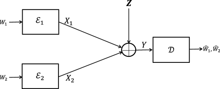
Figure 1: The Gaussian Multiple Access Channel (MAC).

II Lattice Codes

Here, we provide some necessary definitions on lattices and nested lattice codes. Interested reader can refer to [1, 3, 14] and the references therein for more details.

Definition 1.

A lattice $\Lambda$ is a discrete additive subgroup of $\mathbb{R}^{n}$. A lattice $\Lambda$ can always be written in terms of a generator matrix $\mathbf{G}\in\mathbb{R}^{n\times n}$ as $\Lambda=\left\{\boldsymbol{x}=\boldsymbol{z}\mathbf{G}:\boldsymbol{z}\in\mathbb{Z}^{n}\right\},$ where $\mathbb{Z}$ represents the set of integers.

The nearest neighbor quantizer $\mathcal{Q}_{\Lambda}$ maps any point $\boldsymbol{x}\in\mathbb{R}^{n}$ to the nearest lattice point:

$$\mathcal{Q}_{\Lambda}(\boldsymbol{x})=\arg\underset{\boldsymbol{l}\in\Lambda}{\min}\left\|\boldsymbol{x}-\boldsymbol{l}\right\|.$$

The fundamental Voronoi region of lattice $\Lambda$ is set of points in $\mathbb{R}^{n}$ closest to the zero codeword, i.e.,

$$\mathcal{V}_{0}(\Lambda)=\left\{\boldsymbol{x}\in\mathbb{\mathbb{R}}^{n}:\mathcal{Q}(\boldsymbol{x})=0\right\}.$$

$\sigma^{2}\left(\Lambda\right)$ which is called the second moment of lattice $\Lambda$ is defined as

$$\sigma^{2}(\Lambda)=\frac{1}{n}\frac{\int_{\mathcal{V}(\Lambda)}\left\|\boldsymbol{x}\right\|^{2}d\boldsymbol{x}}{\int_{\mathcal{V}(\Lambda)}d\boldsymbol{x}},$$ (1)

and the normalized second moment of lattice $\Lambda$ can be expressed as

$$G(\Lambda)=\frac{\sigma^{2}(\Lambda)}{[\int_{\mathcal{V}(\Lambda)}d\boldsymbol{x}]^{\frac{2}{n}}}=\frac{\sigma^{2}(\Lambda)}{V^{\frac{2}{n}}},$$

where $V=\int_{\mathcal{V}(\Lambda)}d\boldsymbol{x}$ is the Voronoi region volume.

The modulo-$\Lambda$ operation with respect to lattice $\Lambda$ returns the quantization error

$$\boldsymbol{x}\mbox{ mod }\Lambda=\boldsymbol{x}-\mathcal{Q}(\boldsymbol{x}),$$

that maps $\boldsymbol{x}$ into a point in the fundamental Voronoi region and it is always placed in $\mathcal{V}$. The modulo lattice operation satisfies the following distributive property [15]

$$\left[\boldsymbol{x}\mbox{ mod }\Lambda+\boldsymbol{y}\right]\mbox{ mod }\Lambda=\left[\boldsymbol{x}+\boldsymbol{y}\right]\mbox{ mod }\Lambda.$$

(Quantization Goodness or Rogers-good): A sequence of lattices $\Lambda\subseteq\mathbb{R}^{n}$ is good for mean-squared error (MSE) quantization if

$$\underset{n\rightarrow\infty}{\lim}G\left(\Lambda\right)=\frac{1}{2\pi e}.$$

The sequence is indexed by the lattice dimension $n$. The existence of such lattices is shown in [16, 17].

Definition 2.

(AWGN channel coding goodness or Poltyrev-good): Let $\boldsymbol{Z}$ be a length-$i.i.d$ Gaussian vector, $\boldsymbol{Z}\thicksim\mathcal{N}\left(\boldsymbol{0},\sigma_{Z}^{2}\boldsymbol{I}_{n}\right)$. The volume-to-noise ratio of a lattice is given by

$$\mu\left(\Lambda,\epsilon\right)=\frac{\left(\mbox{ Vol}(\mathcal{V})\right)^{2/n}}{2\pi e\sigma_{Z}^{2}},$$

where $\sigma_{Z}^{2}$ is chosen such that $\mbox{ Pr}\left\{\boldsymbol{Z}\notin\mathcal{V}\right\}=\epsilon$ and $\boldsymbol{I}_{n}$ is an $n\times n$ identity matrix. A sequence of lattices is $\Lambda$ Poltyrev-good if

$$\underset{n\rightarrow\infty}{\lim}\mu\left(\Lambda,\epsilon\right)=1,\,\,\,\,\,\forall\epsilon\in\left(0,1\right)$$

and, for fixed volume-to-noise ratio greater than $1$, $\mbox{ Pr}\left\{\boldsymbol{Z}\notin\mathcal{V}\right\}$ decays exponentially in $n$ .

(Nested Lattices): A lattice $\Lambda$ is said to be nested in lattice $\Lambda_{1}$ if $\Lambda\subseteq\Lambda_{1}$. $\Lambda$ is referred to as the coarse lattice and $\Lambda_{1}$ as the fine lattice.

(Nested Lattice Codes): A nested lattice code is the set of all points of a fine lattice $\Lambda_{1}$ that are within the fundamental Voronoi region $\mathcal{V}$ of a coarse lattice $\Lambda$, i.e., $\mathcal{C}=\left\{\Lambda_{1}\cap\mathcal{V}\right\}.$ The rate of a nested lattice code is defined as

$$R=\frac{1}{n}\log\left|\mathcal{C}\right|=\frac{1}{n}\log\frac{\mbox{ Vol}\left(\mathcal{V}\right)}{\mbox{ Vol}\left(\mathcal{V}_{1}\right)}.$$

In [17], Erez, Litsyn and Zamir show that there exists a sequence of lattices that are simultaneously good for packing, covering, source coding (Rogers-good), and channel coding (Poltyrev-good).

III Our Proposed Scheme

As an achievable scheme, we use a lattice-based coding scheme. In [1, 12] by using two nested lattice codes, where one of the lattices provides us codewords while the other lattice satisfies the power constraint at each user, an achievable rate-region for the Ice-Wine problem is established. In fact, the decoder recovers an integer combination of messages. In this paper, we provide a new achievable rate-region for this problem. To reach this goal, we first construct three nested lattices where one of them provides codewords while the other two lattices satisfy the power constraints. At the destination, instead of finding an integer combination of lattice points (or messages), we recover a non-integer linear combination of lattice points. Finally, we apply our proposed scheme to the Gaussian Two-Way Relay Channel (GTWRC) to improve the best rate-region for this open problem so far. Let us consider a standard model of a Gaussian MAC with two users:

$$\boldsymbol{Y}=\boldsymbol{X}_{1}+\boldsymbol{X}_{2}+\boldsymbol{Z},$$ (2)

where $\boldsymbol{Z}$ denotes the AWGN process with zero mean and variance $N$. Each channel input $\boldsymbol{X}_{i}$ is subject to an average power constraint $P$, i.e., $\frac{1}{n}\mathbb{E}\left\|\boldsymbol{X}_{i}\right\|^{2}\leq P$.

In the following, by applying a lattice-based coding scheme, we obtain a new achievable rate-region to estimate a linear combination of messages for the Gaussian MAC. For this purpose, suppose that there exist two lattices $\Lambda_{1}$ and $\Lambda_{2}$, which are Rogers-good (i.e.,$\underset{n\rightarrow\infty}{\lim}G\left(\Lambda_{i}^{(n)}\right)=\frac{1}{2\pi e},\,\textrm{for\,\,\,}i=1,2\,)$, and Poltyrev-good with the following second moments

$$\sigma^{2}\left(\Lambda_{i}\right)=P.$$

Also, there is a lattice $\Lambda_{c}$ which is Poltyrev-good with $\Lambda_{1}\subseteq\alpha_{1}\Lambda_{2}\subseteq\Lambda_{c}$ ($\alpha_{1}$ is a coefficient smaller than one).

Encoding: To transmit both messages, we first construct the following codebooks:

$$\mathcal{C}_{1} = \left\{\Lambda_{c}\cap\mathcal{V}_{1}\right\},\,\,\,\mathcal{C}_{2}=\left\{\frac{\Lambda_{c}}{\alpha_{1}}\cap\mathcal{V}_{2}\right\}.$$

At each encoder, the message set $\left\{1,2,...,2^{nR_{i}}\right\}$ is arbitrarily mapped onto $\mathcal{C}_{i}$ $(i=1,2)$. Then, node $i$ chooses $\boldsymbol{V}_{i}\in\mathcal{C}_{i}$ associated with the message $W_{i}$ and sends

$$\boldsymbol{X}_{i}=\left[\boldsymbol{V}_{i}-\boldsymbol{D}_{i}\right]\textrm{ mod }\Lambda_{i},$$

where $\boldsymbol{D}_{1}$ and $\boldsymbol{D}_{2}$ are two independent dithers that are uniformly distributed over Voronoi regions $\mathcal{V}_{1}$ and $\mathcal{V}_{2}$, respectively. Dithers are known at the encoders and the decoder. Due to the Crypto-lemma [18], $\boldsymbol{X}_{i}$ is uniformly distributed over $\mathcal{V}_{i}$ and independent of $\boldsymbol{V}_{i}$. Thus, the average transmit power of node $i$ equals to $P$, and the power constraint is met.

Decoding: At the decoder, based on the channel output that is given by (2), we estimate

$$\left[\boldsymbol{V}_{1}+\alpha_{1}\boldsymbol{V}_{2}-\alpha_{1}\mathcal{Q}_{\Lambda_{2}}\left(\boldsymbol{V}_{2}-\boldsymbol{D}_{2}\right)\right]\textrm{ mod }\Lambda_{1}.$$

To do this, the decoder performs the following operations:

$$\boldsymbol{Y}_{d} = \left[\alpha_{1}\boldsymbol{Y}+\boldsymbol{D}_{1}+\alpha_{1}\boldsymbol{D}_{2}\right]\textrm{ mod }\Lambda_{1}$$

$$= \left[\alpha_{1}\boldsymbol{X}_{1}+\alpha_{1}\boldsymbol{X}_{2}+\alpha_{1}\boldsymbol{Z}+\boldsymbol{D}_{1}+\alpha_{1}\boldsymbol{D}_{2}\right]\textrm{ mod }\Lambda_{1}$$

$$= \left[\boldsymbol{V}_{1}+\alpha_{1}\boldsymbol{V}_{2}+\alpha_{1}\boldsymbol{X}_{1}-\left(\boldsymbol{V}_{1}-\boldsymbol{D}_{1}\right)\right.$$

$$\left.-\alpha_{1}\mathcal{Q}_{\Lambda_{2}}\left(\boldsymbol{V}_{2}-\boldsymbol{D}_{2}\right)+\alpha_{1}\boldsymbol{Z}\right]\textrm{ mod }\Lambda_{1}$$

$$= \left[\left[\boldsymbol{V}_{1}+\alpha_{1}\boldsymbol{V}_{2}-\alpha_{1}\mathcal{Q}_{\Lambda_{2}}\left(\boldsymbol{V}_{2}-\boldsymbol{D}_{2}\right)\right]\textrm{ mod }\Lambda_{1}\right.$$

$$\left.+(\alpha_{1}-1)\boldsymbol{X}_{1}+\alpha_{1}\boldsymbol{Z}\right]\textrm{ mod }\Lambda_{1}$$

$$= \left[\boldsymbol{T}_{1}+\boldsymbol{Z}_{{\rm eff}}\right]\textrm{ mod }\Lambda_{1},$$

where (III) follows from the distributive law of the modulo operation. The effective noise is given by

$$\boldsymbol{Z}_{{\rm eff}}=\left[(\alpha_{1}-1)\boldsymbol{X}_{1}+\alpha_{1}\boldsymbol{Z}\right]\textrm{ mod }\Lambda_{1},$$

and the sequence to be estimated is given by

$$\boldsymbol{T}_{1}=\left[\boldsymbol{V}_{1}+\alpha_{1}\boldsymbol{V}_{2}-\alpha_{1}\mathcal{Q}_{\Lambda_{2}}\left(\boldsymbol{V}_{2}-\boldsymbol{D}_{2}\right)\right]\textrm{ mod }\Lambda_{1}.$$

Due to the dithers, the vectors $\boldsymbol{V}_{1},\boldsymbol{X}_{1}$ are independent, and also independent of $\boldsymbol{Z}$. Therefore, $\boldsymbol{Z}_{{\rm eff}}$ is independent of $\boldsymbol{V}_{1}$ and $\boldsymbol{V}_{2}$. The decoder attempts to recover $\boldsymbol{T}_{1}$ from $\boldsymbol{Y}_{d}$ instead of recovering $\boldsymbol{V}_{1}$ and $\boldsymbol{V}_{2}$ individually. The method of decoding is minimum Euclidean distance lattice decoding [3, 19], which finds the closest point to $\boldsymbol{Y}_{d}$ in $\Lambda_{c}$. Thus, the estimate of $\boldsymbol{T}_{1}$ is given by

$$\hat{\boldsymbol{T}}_{1}=\mathcal{Q}_{\Lambda_{c}}\left(\boldsymbol{Y}_{d}\right),$$

and the probability of decoding error is given by

$$P_{e} = \textrm{ Pr}\left\{\hat{\boldsymbol{T}}_{1}\neq\boldsymbol{T}_{1}\right\}=\textrm{ Pr}\left\{\boldsymbol{Z}_{{\rm eff}}\notin\mathcal{V}_{c}\right\}.$$

As it is shown in [3] and [19], the error probability vanishes as $n\rightarrow\infty$ if

$$\mu=\frac{\left(\mbox{ Vol}\left(\mathcal{V}_{c}\right)\right)^{\frac{2}{n}}}{2\pi e\textrm{Var}\left(\boldsymbol{Z}_{{\rm eff}}^{*}\right)}>1,$$ (4)

where $\boldsymbol{Z}_{{\rm eff}}^{*}\sim\mathcal{N}\left(0,\textrm{Var}\left(\boldsymbol{Z}_{{\rm eff}}\right)\right)$. Since $\Lambda_{c}$ is Poltyrev-good, the condition of (4) is satisfied. For calculating rate $R_{1}$, we have:

$$R_{1} = \frac{1}{n}\log\left(\frac{\mbox{ Vol}\left(\mathcal{V}_{1}\right)}{\mbox{ Vol}\left(\mathcal{V}_{c}\right)}\right),$$ (5)

$$= \frac{1}{2}\log\left(\frac{\sigma^{2}(\Lambda_{1})}{G(\Lambda_{1})\left(\mbox{ Vol}\left(\mathcal{V}_{c}\right)\right)^{\frac{2}{n}}}\right)$$

$$\leq \frac{1}{2}\log\left(\frac{P}{G(\Lambda_{1})2\pi e\textrm{Var}\left(\boldsymbol{Z}_{{\rm eff}}^{*}\right)}\right)$$

$$\leq \frac{1}{2}\log\left(\frac{{\rm SNR}}{\left(\alpha_{1}-1\right)^{2}{\rm SNR}+\alpha_{1}^{2}}\right)$$ (6)

where (5) follows from (4), and (6) is based on Rogers goodness of $\Lambda_{1}$. Now, for rate $R_{2}$, we have:

$$R_{2} = \frac{1}{n}\log\left(\frac{\alpha_{1}^{n}\mbox{ Vol}\left(\mathcal{V}_{2}\right)}{\mbox{ Vol}\left(\mathcal{V}_{c}\right)}\right)$$

$$= \frac{1}{n}\log\left(\frac{\alpha_{1}^{n}\mbox{ Vol}\left(\mathcal{V}_{2}\right)}{\mbox{ Vol}\left(\mathcal{V}_{1}\right)}\right)+\frac{1}{n}\log\left(\frac{\mbox{ Vol}\left(\mathcal{V}_{1}\right)}{\mbox{ Vol}\left(\mathcal{V}_{c}\right)}\right)$$

$$= \frac{1}{2}\log\left(\frac{G(\Lambda_{1})\alpha_{1}^{2}\sigma^{2}\left(\Lambda_{2}\right)}{G(\Lambda_{2})\sigma^{2}\left(\Lambda_{1}\right)}\right)+R_{1}$$

$$= R_{1}+\frac{1}{2}\log\left(\alpha_{1}^{2}\right)$$

$$\leq \frac{1}{2}\log\left(\frac{\alpha_{1}^{2}{\rm SNR}}{\left(\alpha_{1}-1\right)^{2}{\rm SNR}+\alpha_{1}^{2}}\right),$$ (8)

where (III) follows from the fact that lattices $\Lambda_{1}$ and $\Lambda_{2}$ are Rogers-good. Thus, to estimate $\boldsymbol{T}_{1}$ correctly, from (6) and (8), we get the rate-region $\mathcal{R}_{1}\left(\alpha_{1}\right)$, where

$$\mathcal{R}_{1}\left(\alpha_{1}\right)= \left\{\left(R_{1},R_{2}\right):\,\,R_{1}\leq\frac{1}{2}\log\left(\frac{{\rm SNR}}{\left(\alpha_{1}-1\right)^{2}{\rm SNR}+\alpha_{1}^{2}}\right)\right.$$ (9)

$$\left.R_{2}\leq\frac{1}{2}\log\left(\frac{\alpha_{1}^{2}{\rm SNR}}{\left(\alpha_{1}-1\right)^{2}{\rm SNR}+\alpha_{1}^{2}}\right)\right\}.$$

Thus, we have proved the following Theorem which is one of the main contributions of this paper.

Theorem 1.

For the Gaussian MAC shown in Fig. 1, if any rate pair $\left(R_{1},R_{2}\right)$ satisfies the rate constraints given in (9), then, there exist sequences of nested lattices $\Lambda_{1}\subseteq\frac{\Lambda_{2}}{\alpha_{1}}\subseteq\Lambda_{c}$ such that the following linear combination can be recovered:

$$\left[\boldsymbol{V}_{1}+\alpha_{1}\boldsymbol{V}_{2}-\alpha_{1}\mathcal{Q}_{\Lambda_{2}}\left(\boldsymbol{V}_{2}-\boldsymbol{D}_{2}\right)\right]\textrm{ mod }\Lambda_{1},$$

where $0\leq\alpha_{1}\leq 1$.

Now, by exchanging the role of two encoders in the preceding theorem and by following the above-mentioned steps, we can show that if

$$\mathcal{R}_{2}\left(\alpha_{2}\right)= \left\{\left(R_{1},R_{2}\right):\,\,R_{1}\leq\frac{1}{2}\log\left(\frac{\alpha_{2}^{2}{\rm SNR}}{\left(\alpha_{2}-1\right)^{2}{\rm SNR}+\alpha_{2}^{2}}\right)\right.$$ (10)

$$\left.\qquad R_{2}\leq\frac{1}{2}\log\left(\frac{{\rm SNR}}{\left(\alpha_{2}-1\right)^{2}{\rm SNR}+\alpha_{2}^{2}}\right)\right\},\quad$$

$$0\leq\alpha_{2}\leq 1$$

then, we can correctly recover the following linear combination at the destination:

$$\boldsymbol{T}_{2}=\left[\boldsymbol{V}_{2}+\alpha_{2}\boldsymbol{V}_{1}-\alpha_{2}\mathcal{Q}_{\Lambda_{1}}\left(\boldsymbol{V}_{1}-\boldsymbol{D}_{1}\right)\right]\textrm{ mod }\Lambda_{2}.$$

In Fig. 2, we compare the achievable rate-regions for estimating these two linear combinations with the outer bound.

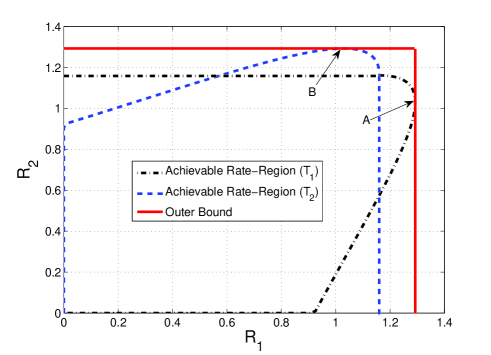
Figure 2: The achievable rate-region in order to estimate $\boldsymbol{T}_{1}$ and $\boldsymbol{T}_{2}$. As we observe, the proposed scheme can reach to the outer bound at points $A$ and $B$. The signal-to-noise ratio is fixed at $SNR=5$.

Remark 1.

Note that by replacing $\alpha_{1}$ and $\alpha_{2}$ with $\alpha_{{}_{{\rm MMSE}}}=\frac{{\rm SNR}}{1+{\rm SNR}}$ in the rate-regions $\mathcal{R}_{1}\left(\alpha_{1}\right)$ and $\mathcal{R}_{2}\left(\alpha_{2}\right)$, given in (9) and (10), we can see that the following points are achievable:

$$A = \left(\frac{1}{2}\log\left(1+{\rm SNR}\right),\frac{1}{2}\log\left(\frac{{\rm SNR}^{2}}{1+{\rm SNR}}\right)\right)$$

$$B = \left(\frac{1}{2}\log\left(\frac{{\rm SNR}^{2}}{1+{\rm SNR}}\right),\frac{1}{2}\log\left(1+{\rm SNR}\right)\right).$$

On the other hand, achieving the sum of codewords over the Gaussian MAC can be upper bounded by the following rate region:

$$R_{1} \leq \frac{1}{2}\log\left(1+{\rm SNR}\right),\,\,\,\,R_{2}\leq\frac{1}{2}\log\left(1+{\rm SNR}\right).$$

Thus, by comparing this outer bound with our achievable rate region, we observe that it always coincides with the outer bound for each linear combination.

Achieving linear combination of codewords at the Gaussian MAC has many applications in network information theory, see e.g. [2, 1, 12]. In all these papers, achieving $\left[\boldsymbol{V}_{1}+\boldsymbol{V}_{2}\right]\textrm{ mod }\Lambda_{1}$ is studied and it is shown that the following rate region is achievable:

$$R_{i} \leq \frac{1}{2}\log\left(\frac{1}{2}+{\rm SNR}\right),\,\,\,\,\,(i=1,2).$$ (11)

By comparing the achievable rate region of the compute-and-forward scheme, given in (11), with the outer bound, it is clear that the compute-and-forward scheme is not able to coincide with the outer bound even partially whereas our achievable rate-region for estimating $\boldsymbol{T}_{1}$ or $\boldsymbol{T}_{2}$ is partially tight.

Remark 2.

Here, we compare our proposed scheme for the Ice-Wine problem with the proposed schemes in [1, 2, 12]. In these papers, using the fact that each integer linear combination of lattice points is another lattice point, the given rate-region in (11) is established. As we see, there is a loss of $\frac{1}{2}$ bit compared with the outer bound. But, where is the source of this loss?

To achieve $\left[\boldsymbol{V}_{1}+\boldsymbol{V}_{2}\right]\textrm{ mod }\Lambda$, we are forced to have the following effective noise:

$$\boldsymbol{Z}_{{\rm eff}}=\left[\left(\alpha-1\right)\left(\boldsymbol{X}_{1}+\boldsymbol{X}_{2}\right)+\alpha\boldsymbol{Z}\right]\textrm{ mod }\Lambda.$$

We see that both terms $\boldsymbol{X}_{1}$ and $\boldsymbol{X}_{2}$ are presented in the effective noise. This yields the loss of $\frac{1}{2}$ bit. However, in our proposed scheme, we try to eliminate $\boldsymbol{X}_{2}$ at the effective noise. This helps us to achieve full capacity for one user but due to the chosen codebooks at the transmitter side, we cannot achieve the full rate for the other user.

IV The Gaussian Two-Way Relay Channel

One can apply the proposed scheme in this paper to the Gaussian Two-Way Relay Channel (GTWRC) to improve the best rate region of this channel, provided in [11]. The following Theorem provides this rate-region.

Theorem 2.

For the Gaussian two-way relay channel, if both transmitters transmit at equal powers, then the following rate-region is achievable:

$$\mathcal{R}=\textrm{cl conv}\left\{\left(\underset{\alpha_{1}\in\left[0,1\right]}{\bigcup}\mathcal{R}_{1}\left(\alpha_{1}\right)\right)\bigcup\left(\underset{\alpha_{2}\in\left[0,1\right]}{\bigcup}\mathcal{R}_{2}\left(\alpha_{2}\right)\right)\right\},$$ (12)

where $\mathcal{R}_{1}\left(\alpha_{1}\right)$ and $\mathcal{R}_{2}\left(\alpha_{2}\right)$ are defined in (9) and (10), respectively. Also, cl and conv are the closure and the convex hull operations, respectively.

Proof:

For this purpose, node $i$ constructs the following sequence and sends it over the channel:

$$\boldsymbol{X}_{i}=\left[\boldsymbol{V}_{i}-\boldsymbol{D}_{i}\right]\textrm{ mod }\Lambda_{i},\qquad i=1,2$$

Then, by our proposed scheme, we can estimate the linear combination, $\boldsymbol{T}_{1}$ or $\boldsymbol{T}_{2}$, at the relay node. In the following, without loss of generality, assume that we estimate $\boldsymbol{T}_{1}$, given as

$$\boldsymbol{T}_{1}=\left[\boldsymbol{V}_{1}+\alpha_{1}\boldsymbol{V}_{2}-\alpha_{1}\mathcal{Q}_{\Lambda_{2}}\left(\boldsymbol{V}_{2}-\boldsymbol{D}_{2}\right)\right]\textrm{ mod }\Lambda_{1}.$$

Now, the relay node, using random coding sends $\boldsymbol{T}_{1}$ to both nodes as it is explained in [11]. At node 1, we know $\boldsymbol{V}_{1}$. Thus, we estimate $\boldsymbol{V}_{2}$ as the following:

$$\widehat{\boldsymbol{V}_{2}} = \frac{1}{\alpha_{1}}\left[\boldsymbol{T}_{1}-\boldsymbol{v}_{1}\right]\textrm{ mod }\Lambda_{3}$$

$$= \frac{1}{\alpha_{1}}\left[\alpha_{1}\boldsymbol{V}_{2}-\alpha_{1}\mathcal{Q}_{\Lambda_{2}}\left(\boldsymbol{V}_{2}-\boldsymbol{D}_{2}\right)\right]\textrm{ mod }\Lambda_{3}$$

$$= \frac{1}{\alpha_{1}}\left[\alpha_{1}\boldsymbol{V}_{2}\right]\textrm{ mod }\Lambda_{3}=\boldsymbol{V}_{2}.$$

Similarly, node 2 with knowing $\boldsymbol{V}_{2}$, estimates message of node 1. Thus, we can achieve the rate-region $\mathcal{R}_{1}\left(\alpha_{1}\right)$ for the GTWRC. On the other hand, by finding $\boldsymbol{T}_{2}$ at the relay node, we can see that the rate-region $\mathcal{R}_{2}\left(\alpha_{2}\right)$ is also achievable. Finally, using time-sharing between these two rate-regions, we get the entire achievable rate-region $\mathcal{R}$ in (12). ∎

As a numerical example, in Figs. 3 and 4, we compare the achievable rate-region of our proposed scheme with that of the compute-and-forward scheme. For comparison, an outer bound is also provided. As we observe, our proposed scheme can achieve the outer bound and thus capacity region is partially known. By increasing SNR, the gap between our proposed scheme with the outer bound is reduced. In these Figures, we also depict the convex hull of our achievable rate-region and the achievable rate-region by the compute-and-forward scheme. To the best of our knowledge, this rate region is the best rate region for the Gaussian TWRC so far.

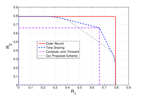
Figure 3: Achievable rate-regions and rate-region outer bound for ${\rm SNR}=2$.

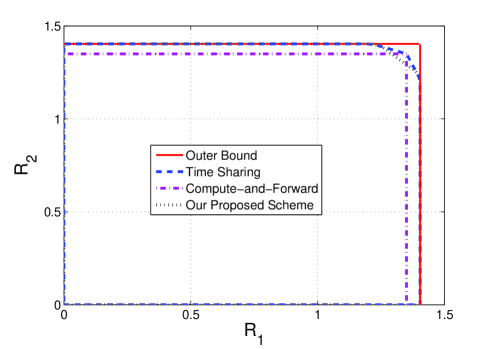
Figure 4: Achievable rate-regions and rate-region outer bound for ${\rm SNR}=6$.

V Conclusion

In this paper, we studied the Ice-Wine problem and using nested lattice codes, we obtained a new achievable rate-region for this problem. In contrast with the previous obtained achievable rate regions, the achievable rate-region achieves the outer bound partially for each user. As we observed, our proposed scheme achieves some rates which are not achievable by all known schemes to date. Finally, using applying our proposed scheme to the GTWRC, we showed that the best achievable rate-region for this open problem can be improved significantly.

References

- [1] B. Nazer and M. Gastpar, “Compute-and-forward: Harnessing interference through structured codes,” IEEE Trans. Inf. Theory, vol. 57, no. 10, pp. 6463–6486, Oct. 2011.
- [2] M. P. Wilson, K. Narayanan, H. Pfister, and A. Sprintson, “Joint physical layer coding and network coding for bidirectional relaying,” IEEE Trans. Inf. Theory, vol. 56, no. 11, pp. 5641– 5654, Nov. 2010.
- [3] U. Erez and R. Zamir, “Achieving 1/2 log(1 +SNR) on the AWGN channel with lattice encoding and decoding,” IEEE Trans. Inf. Theory, vol. 50, no. 22, pp. 2293–2314, Oct. 2004.
- [4] R. Zamir, S. Shamai, and U. Erez, “Nested linear/lattice codes for structured multiterminal binning,” IEEE Trans. Inf. Theory, vol. 48, no. 6, pp. 1250–1276, Jun. 2002.
- [5] Y. Song and N. Devroye, “Lattice codes for the Gaussian relay channel: Decode-and-forward and compress-and-forward,” IEEE Trans. Inf. Theory, vol. 59, no. 8, pp. 4927–4948, Aug. 2013.
- [6] R. Ahlswede, “Multiway communication channels,” in Proc. 2nd Int. Symp. Inf. Theory, Tsahkadsor, USA, 1971, pp. 23–52.
- [7] M. Gastpar and B. Nazer, “Algebraic structure in network information theory,” [Online]. Available: http://iss.bu.edu/bobak/tutorial_isit11.pdf.
- [8] P. Popovski and H. Yomo, “Physical network coding in two-way wireless relay channels,” in Proc. IEEE Int. Conf. Commun. (ICC), 2007, pp. 707–712.
- [9] J. Zhan, B. Nazer, U. Erez, and M. Gastpar, “Integer-forcing linear receivers,” To appear at IEEE Trans. Inf. Theory, arXiv:1003.5966, Aug. 2014.
- [10] O. Ordentlich, U. Erez, and B. Nazer, “Successive integer-forcing and its sum-rate optimality,” in Proc. 51th Allerton Conf. Commun., Contr., Comput., Urbana, Illinois, Sep. 2013.
- [11] W. Nam, S.-Y. Chung, and Y. H.Lee, “Capacity of the Gaussian Two-Way relay channel to within 1/2 bit,” IEEE Trans. Inf. Theory, vol. 56, no. 11, pp. 5488–5494, Nov. 2010.
- [12] ——, “Nested lattice codes for Gaussian relay networks with interference,” IEEE Trans. Inf. Theory, vol. 57, no. 12, pp. 7733 – 7745, Dec. 2011.
- [13] J. Zhu and M. Gastpar, “Asymmetric compute-and-forward with csit,” in Proceedings of the 23nd International Zurich Seminar on Communication (IZS 2014), Zurich, Switzerland, Feb. 2014.
- [14] J. H. Conway and N. J. A. Sloane, Sphere Packings, Lattices and Groups. New York: Springer-Verlag, 1992.
- [15] B. Nazer and M. Gastpar, “Computation over multiple-access channels,” IEEE Trans. Inf. Theory, vol. 53, no. 19, pp. 3498 – 3516, Oct. 2007.
- [16] R. Zamir and M. Feder, “On lattice quantization noise,” IEEE Trans. Inf. Theory, vol. 42, no. 4, pp. 1152–1159, Jul. 1996.
- [17] U. Erez, S. Litsyn, and R. Zamir, “Lattices which are good for (almost) everything,” IEEE Trans. Inf. Theory, vol. 51, no. 16, pp. 3401–3416, Oct. 2005.
- [18] G. D. Forney, “On the role of MMSE estimation in approaching the information theoretic limits of linear Gaussian channels: Shannon meets Wiener,” in Proc. 41st Ann. Allerton Conf., Monticello, IL, Oct. 2003.
- [19] G. Poltyrev, “On coding without restrictions for the AWGN channel,” IEEE Trans. Inf. Theory, vol. 40, no. 9, pp. 409 – 417, Mar. 1994.