Building relativistic mean field models for finite nuclei and neutron stars

Abstract

Background

Theoretical approaches based on density functional theory provide the only tractable method to incorporate the wide range of densities and isospin asymmetries required to describe finite nuclei, infinite nuclear matter, and neutron stars.

Purpose

A relativistic energy density functional (EDF) is developed to address the complexity of such diverse nuclear systems. Moreover, a statistical perspective is adopted to describe the information content of various physical observables.

Methods

We implement the model optimization by minimizing a suitably constructed ${\chi}^{\raisebox{-1.0pt}{$\scriptstyle{2}$}}$ objective function using various properties of finite nuclei and neutron stars. The minimization is then supplemented by a covariance analysis that includes both uncertainty estimates and correlation coefficients.

Results

A new model, “FSUGold 2”, is created that can well reproduce the ground-state properties of finite nuclei, their monopole response, and that accounts for the maximum neutron star mass observed up to date. In particular, the model predicts both a stiff symmetry energy and a soft equation of state for symmetric nuclear matter—suggesting a fairly large neutron-skin thickness in ²⁰⁸Pb and a moderate value of the nuclear incompressibility.

Conclusions

We conclude that without any meaningful constraint on the isovector sector, relativistic EDFs will continue to predict significantly large neutron skins. However, the calibration scheme adopted here is flexible enough to create models with different assumptions on various observables. Such a scheme—properly supplemented by a covariance analysis—provides a powerful tool to identify the critical measurements required to place meaningful constraints on theoretical models.

I Introduction

Finite nuclei, infinite nuclear matter, and neutron stars are complex, many-body systems governed largely by the strong nuclear force. Although Quantum Chromodynamics (QCD) is the fundamental theory of the strong interaction, enormous challenges have prevented us from solving the theory in the non-perturbative regime of relevance to nuclear systems. To date, these complex systems can be investigated only in the framework of an effective theory with appropriate degrees of freedom. Among the effective approaches, the one based on density functional theory (DFT) is most promising, as it is the only microscopic approach that may be applied to the entire nuclear landscape and to neutron stars. In the past decades numerous energy density functionals (EDFs) have been proposed which can be grouped into two main branches: non-relativistic and relativistic. Skyrme-type functionals are the most popular ones within the non-relativistic domain, where nucleons interact via density-dependent effective potentials. Using such a framework, the Universal Nuclear Energy Density Functional (UNEDF) Collaboration UNE aims to achieve a comprehensive understanding of finite nuclei and the reactions involving them Kortelainen et al. (2010a, 2012, 2013). On the other end, relativistic mean field (RMF) models, based on a quantum field theory having nucleons interacting via the exchange of various mesons, have been successfully used since the 1970’s and provide a covariant description of both infinite nuclear matter and finite nuclei Walecka (1974); Serot and Walecka (1986); Horowitz and Serot (1981); Lalazissis et al. (1997, 1999); Todd-Rutel and Piekarewicz (2005).

In the traditional spirit of effective theories, both non-relativistic and relativistic EDFs are calibrated from nuclear experimental data that is obtained under normal laboratory conditions, namely, at or slightly below nuclear saturation density and with small to moderate isospin asymmetries. The lack of experimental data at both higher densities and with extreme isospin asymmetries leads to a large spread in the predictions of the models—even when they may all be calibrated to the same experimental data. Consequently, fundamental nuclear properties, such as the neutron density of medium-to-heavy nuclei Brown (2000); Furnstahl (2002); Centelles et al. (2009); Roca-Maza et al. (2011), proton and neutron drip lines Erler et al. (2012); Afanasjev et al. (2013), and a variety of neutron star properties Lattimer and Prakash (2004); Demorest et al. (2010); Antoniadis et al. (2013) remain largely undetermined.

It has been a common practice for a long time to supplement experimental results with uncertainty estimates. Indeed, no experimental measurement could ever be published without properly estimated “error bars”. Often, the most difficult part of an experiment is a reliable quantification of systematic errors and improving the precision of the measurement consists of painstaking efforts at reducing the sources of such uncertainties. On the contrary, theoretical predictions merely involve reporting a “central value” without any information on the uncertainties inherent in the formulation or the calculation. Thus, to determine whether a theory is successful or not, the only required criterion is to reproduce the experimental data. Although this approach has certain value—especially if the examined model reproduces a vast amount of experimental data—such a criterion is often neither helpful nor meaningful. And the situation becomes even worse if the predictions of an effective theory are extrapolated into unknown regions, such as the boundaries of the nuclear landscape and the interior of neutron stars. How can a model provide experimental or observational guidance without supplementing its predictions with theoretical errors? In recent years, “the importance of including uncertainty estimates in papers involving theoretical calculations of physical quantities” has been underscored Editors (2011). This is particularly critical when theoretical models are used to extrapolate experimental data to uncharted regions of the observable landscape. Thus, theoretical uncertainty estimates are critical in assessing the reliability of the extrapolations. Moreover, if these theoretical errors are large, then one can perform a correlation analysis to uncover observables that can help reduce the size of the uncertainties. Several manuscripts highlighting the role of information and statistics in nuclear physics have been published recently Reinhard and Nazarewicz (2010); Fattoyev and Piekarewicz (2011, 2012); Reinhard and Nazarewicz (2013); Reinhard et al. (2013); Dobaczewski et al. (2014); Piekarewicz et al. (2014). Moreover, at the time of this writing, a focus issue devoted to “Enhancing the interaction between nuclear experiment and theory through information and statistics” was under development.

In this work we develop a modeling scheme within the framework of the RMF theory that consists of both the optimization of a theoretical model and the follow-up covariance analysis. However, unlike the UNEDF Collaboration, our goals are rather modest as we do not attempt to study all the facets of finite nuclei. Instead, we limit ourselves to a treatment of the ground-state properties of magic (or semi-magic) finite nuclei, centroid energies of monopole resonances, and properties of neutron stars. We would like to emphasize that all the data that we use in the optimization of the relativistic EDF consists of real physical observables without any reliance on bulk properties of infinite nuclear matter. This is now possible due to the remarkable advances in land- and space-based telescopes that have started to place meaningful constraints on the high-density component of the equation of state. In particular, observations made with the Green Bank Telescope have provided highly precise measurements of two massive (of about 2 $M_{\odot}$) neutron stars Demorest et al. (2010); Antoniadis et al. (2013). Further, an enormous effort is also being devoted to the extraction of stellar radii from x-ray observations Ozel et al. (2010); Steiner et al. (2010); Suleimanov et al. (2011); Guillot et al. (2013). Such astronomical observations will be instrumental in constraining the nuclear EDF in regions inaccessible to laboratory experiments.

Not having to rely on the bulk properties of nuclear matter in the calibration procedure implies that these properties now become genuine model predictions—with associated theoretical errors—that may be compared against results from ab initio calculations or other microscopic approaches Schwenk and Pethick (2005); Gezerlis and Carlson (2010); Vidana et al. (2009); Hebeler et al. (2010, 2013). Although not directly measurable, a determination of the bulk properties of infinite nuclear matter provides valuable constraints on the equation of state (EOS) of dense neutron-rich matter. Moreover, some of these critical parameters are known to be strongly correlated to observables that may be directly measured. This fact provides a powerful bridge between observation, experiment, and theory. However, until very recently most of these correlations were inferred by comparing a large set of EDFs; see Ref. Roca-Maza et al. (2011) for a particularly illustrative example. Although such an analysis provides critical insights into the systematic errors associated with the biases and limitations of each model, it is essential that it be supplemented with a proper statistical analysis. Indeed, such a covariance analysis represents the least biased and most reliable approach to uncover correlations among physical observables Reinhard and Nazarewicz (2010); Fattoyev and Piekarewicz (2011, 2012); Reinhard and Nazarewicz (2013); Reinhard et al. (2013); Dobaczewski et al. (2014); Piekarewicz et al. (2014).

The paper has been organized as follows. Following this introduction, we outline the theoretical framework in Sec. II. We follow closely the approach developed in Ref. Piekarewicz et al. (2014) that starts from a gaussian approximation to a suitably defined likelihood function. To demonstrate the power of the approach, we construct in Sec. III a brand new functional (FSUGold 2) that is calibrated from the ground-state properties of finite nuclei, their isoscalar monopole response, and a maximum neutron star mass. Finally, we conclude with a summary and outlook in Sec. IV.

II Theoretical Framework

In this section we outline the theoretical framework required to accurately calibrate an energy density functional. The section itself is divided into three components. First, we introduce the RMF model that will be used to compute all required nuclear properties—from finite nuclei to neutron stars. Second, we develop, to our knowledge for the first time in the RMF context, a transformation that links the model parameters to “pseudo data” given in the form of bulk properties of infinite nuclear matter. Such a transformation enables us to implement the optimization in the space of pseudo data, resulting in a more intuitive and more efficient approach. Finally, in the third and last subsection we describe details of the optimization procedure followed by a covariance analysis that is used to estimate both theoretical uncertainties and correlations among observables.

II.1 Relativistic Mean Field Theory

In the framework of the RMF theory, the basic degrees of freedom include nucleons (protons and neutrons), three “mesons”, and the photon. The nucleons are the constituents of the nuclear many-body system, which interact via the transfer of the force carriers, with the various mesons conveying the strong force between the nucleons and the photons mediating the additional electromagnetic force between the protons. The interactions among the particles can be depicted by an effective Lagrangian density of the following form Walecka (1974); Serot and Walecka (1986); Mueller and Serot (1996); Serot and Walecka (1997); Horowitz and Piekarewicz (2001a):

$${\mathscr{L}}_{\rm int} = \bar{\psi}\left[g_{\rm s}\phi\!-\!\left(g_{\rm v}V_{\mu}\!+\!\frac{g_{\rho}}{2}{\mbox{\boldmath$\tau$}}\cdot{\bf b}_{\mu}\!+\!\frac{e}{2}(1\!+\!\tau_{3})A_{\mu}\right)\gamma^{\mu}\right]\psi$$ (1)

$$- \frac{\kappa}{3!}(g_{\rm s}\phi)^{3}\!-\!\frac{\lambda}{4!}(g_{\rm s}\phi)^{4}\!+\!\frac{\zeta}{4!}g_{\rm v}^{4}(V_{\mu}V^{\mu})^{2}+\Lambda_{\rm v}\Big{(}g_{\rho}^{2}\,{\bf b}_{\mu}\cdot{\bf b}^{\mu}\Big{)}\Big{(}g_{\rm v}^{2}V_{\nu}V^{\nu}\Big{)}\;,$$

where $\psi$ is the isodoublet nucleon field, $A_{\mu}$ is the photon field, and $\phi$, $V_{\mu}$, and ${\bf b}_{\mu}$ represent the isoscalar-scalar $\sigma$-, isoscalar-vector $\omega$-, and isovector-vector $\rho$-meson field, respectively. The first line of the above equation contains the conventional Yukawa couplings between the nucleons and the mesons, while the second line includes some nonlinear self and mixed interactions between the mesons. In the spirit of an effective field theory, one should incorporate all possible meson interactions that are allowed by symmetry considerations to a given order in a power-counting scheme. Moreover, once the dimensionful meson fields have been properly scaled using strong-interaction mass scales, the remaining dimensionless coefficients of the effective Lagrangian should all be “natural”, namely, of order one (i.e., neither too small nor too large) Furnstahl et al. (1997a, b); Rusnak and Furnstahl (1997); Furnstahl and Hackworth (1997); Kortelainen et al. (2010b). However, given the limited experimental database of nuclear observables, certain empirical coefficients—or linear combinations of them—may remain poorly constrained after the optimization procedure. This results in “unnatural” coefficients that deviate significantly from unity. Therefore, in an effort to avoid this problem only a subset of nonlinear meson interactions is retained in the formalism. For instance, in the interaction Lagrangian density depicted in Eq. (1), one only keeps the four meson interactions denoted by the coefficients: $\kappa$, $\lambda$, $\zeta$, and $\Lambda_{\rm v}$. In particular, these terms are found to have a clear physical connection to various properties of the nuclear equation of state. Two of the isoscalar parameters, $\kappa$ and $\lambda$, were introduced by Boguta and Bodmer Boguta and Bodmer (1977) to reduce the nuclear incompressibility coefficient of symmetric nuclear matter from an unreasonably large value in the original Walecka model Walecka (1974); Serot and Walecka (1986) to one that can be made consistent with measurements of giant monopole resonances in finite nuclei. In turn, $\zeta$ may be used to efficiently tune the maximum neutron star mass without sacrificing the agreement with other well reproduced observables Mueller and Serot (1996). Finally, $\Lambda_{\rm v}$ is highly sensitive to the density dependence of symmetry energy—and in particular to its slope at saturation density—which has important implications in the structure and dynamics of neutron stars Horowitz and Piekarewicz (2001a, b); Carriere et al. (2003); Horowitz et al. (2004).

With the Lagrangian density given in Eq. (1), one can derive the equation of motion for each of the constituent particles in the mean-field limit Todd and Piekarewicz (2003). The nucleons satisfy a Dirac equation in the presence of mean-field potentials having Lorentz scalar and vector character. In turn, the various mesons satisfy nonlinear and inhomogeneous Klein-Gordon equations with the various nuclear densities acting as source terms. Lastly, the photon obeys the Poisson equation with the proton density being the relavant source term. Given that the nuclear densities act as sources for the meson fields and, in turn, the meson fields determine the mean-field potentials for the nucleons, the set of equations must be solved self-consistently. Once solved, these equations determine the ground-state properties of the nucleus of interest—such as its total binding energy, single-nucleon energies and wave functions, distribution of meson fields, and density profiles.

The solution of the mean-field equations is simplified significantly in the case of infinite nuclear matter, which we assume to be spatially uniform. For this uniform case, the meson fields are uniform (i.e., constant throughout space) and the nucleon orbitals are plane-wave Dirac spinors with medium-modified effective masses and energies. By forming the energy-momentum tensor in the mean-field approximation Serot and Walecka (1986), one can readily infer (in the rest frame of the fluid) the energy density and pressure of the system as a function of the conserved baryon density $\rho\!=\rho_{n}\!+\!\rho_{p}$ and the neutron-proton asymmetry $\alpha\!\equiv\!(\rho_{n}\!-\!\rho_{p})/(\rho_{n}\!+\!\rho_{p})$. In particular, the energy per nucleon of the system may be expanded in even powers of $\alpha$. That is,

$$\frac{E}{A}(\rho,\alpha)-\!M\equiv{\cal E}(\rho,\alpha)={\cal E}_{\rm SNM}(\rho)+\alpha^{2}{\cal S}(\rho)+{\cal O}(\alpha^{4})\,,$$ (2)

where ${\cal E}_{\rm SNM}(\rho)\!=\!{\cal E}(\rho,\alpha\!\equiv\!0)$ is the energy per nucleon of symmetric nuclear matter (SNM) and the symmetry energy ${\cal S}(\rho)$ represents the first-order correction to the symmetric limit. Note that no odd powers of $\alpha$ appear as the nuclear force is assumed to be isospin symmetric and electromagnetic effects have been “turned off”. Also note that, although model dependent, to a very good approximation the symmetry energy has a very intuitive interpretation: it represents the energy cost required to convert symmetric nuclear matter into pure neutron matter (PNM):

$${\cal S}(\rho)\!\approx\!{\cal E}(\rho,\alpha\!=\!1)\!-\!{\cal E}(\rho,\alpha\!=\!0)\;.$$ (3)

It is also customary to characterize the behavior of both symmetric nuclear matter and the symmetry energy in terms of a few bulk parameters. To do so, we perform a Taylor series expansion around nuclear matter saturation density $\rho_{\raisebox{-0.75pt}{\tiny 0}}$. That is Piekarewicz and Centelles (2009),

$${\cal E}_{\rm SNM}(\rho)=\varepsilon_{\raisebox{-0.75pt}{\tiny 0}}+\frac{1}{2}Kx^{2}+\ldots,$$ (4a)

$${\cal S}(\rho)=J+Lx+\frac{1}{2}K_{\rm sym}x^{2}+\ldots,$$ (4b)

​​​where $x\!=\!(\rho-\rho_{\raisebox{-0.75pt}{\tiny 0}})\!/3\rho_{\raisebox{-0.75pt}{\tiny 0}}$ is a dimensionless parameter that quantifies the deviations of the density from its value at saturation. Here $\varepsilon_{\raisebox{-0.75pt}{\tiny 0}}$ and $K$ represent the energy per nucleon and the incompressibility coefficient of SNM; $J$ and $K_{\rm sym}$ are the corresponding quantities for the symmetry energy. However, unlike symmetric nuclear matter whose pressure vanishes at $\rho_{\raisebox{-0.75pt}{\tiny 0}}$, the slope of the symmetry energy $L$ does not vanish at saturation density. Indeed, assuming the validity of Eq. (3), $L$ is directly proportional to the pressure of PNM ($P_{0}$) at saturation density, namely,

$$P_{0}\approx\frac{1}{3}\rho_{\raisebox{-0.75pt}{\tiny 0}}L\;.$$ (5)

Finally, one can go a step further and apply the above formalism to neutron star matter, which we assume to consist of neutrons, protons, electrons, and muons in $\beta$ equilibrium. Note that no “exotic” degrees of freedom—such as hyperons, meson condensates, or quarks—are included in the formalism. At the densities at which neutron star matter is uniform, electrons and muons may be treated as relativistic Fermi gases that contribute to the total energy density and pressure of the system. In $\beta$ equilibrium only the baryon density needs to be specified, as the neutron-proton asymmetry is adjusted to minimize the total energy density of the system. Given that uniform neutron-rich matter is unstable against cluster formation, we supplement our RMF predictions for the EOS with the standard parametrization for the outer crust by Baym, Pethick, and Sutherland Baym et al. (1971). Finally, we resort to a polytropic EOS to interpolate between the solid outer crust and the uniform liquid core Link et al. (1999); Carriere et al. (2003). Given that the EOS is the only input required to solve the Tolman-Oppenheimer-Volkoff equation, one can predict a variety of neutron star properties that can then be compared against observation. Particularly relevant in this work will be the predictions for the maximum stellar mass and the radius of a “canonical” 1.4 $M_{\odot}$ neutron star.

II.2 An Insightful Transformation

The main goal of the present work is the accurate calibration of a relativistic EDF by relying exclusively on measured properties of finite nuclei and neutron stars. The fitting protocol requires both the specification of a theoretical model and the selection of physical observables to constrain the fit. The conventional approach to the calibration of the EDF consists of first minimizing the objective function and then validating the model against observables not included in the fit. Traditionally, the optimization of the model is carried out in parameter space. That is, one searches for those model parameters (e.g., $g_{\rm s},g_{\rm v},\ldots$) that minimize the objective function. Given that the connection between the model parameters and our physical intuition is tenuous at best, the searching algorithm often ends up wandering aimlessly in search of the minimum. A remarkable, but little known, fact in the framework of the RMF theory is that many of the model parameters can be expressed in terms of a few bulk properties of infinite nuclear matter Glendenning (2000). Although relatively new, it appears that such a transformation between the model parameters and the bulk properties of infinite nuclear matter (or “pseudo data”) is better known in the case of the non-relativistic Skyrme interaction Agrawal et al. (2005); Chen et al. (2010); Kortelainen et al. (2010a). To avoid interrupting the flow of the narrative, we only summarize here the central points of the transformation. A detailed account of the transformation has been reserved to the appendix.

For the Lagrangian density given in Eq. (1), we identify five isoscalar ($g_{\rm s},g_{\rm v},\kappa,\lambda$, and $\zeta$) and two isovector ($g_{\rho}$ and $\Lambda_{\rm v}$) parameters. Note that in a mean-field approximation, the properties of infinite nuclear matter are only sensitive to the combinations $g_{\rm s}^{2}/m_{\rm s}^{2}$, $g_{\rm v}^{2}/m_{\rm v}^{2}$, and $g_{\rho}^{2}/m_{\rho}^{2}$. The transformation starts in the isoscalar sector and links the first four isoscalar parameters listed above with four bulk properties of symmetric nuclear matter; these are the density $\rho_{\raisebox{-0.75pt}{\tiny 0}}$, the binding energy per nucleon $\varepsilon_{\raisebox{-0.75pt}{\tiny 0}}$, the effective nucleon mass $M^{\ast}$, and the incompressibility coefficient $K$—all evaluated at saturation density. The fact that the pressure of SNM vanishes at saturation density implies, through the Hugenholtz-van Hove theorem, that the energy per nucleon must equal the nucleon Fermi energy. This fact, together with the classical equation of motion for the vector field, is sufficient to determine $g_{\rm v}^{2}/m_{\rm v}^{2}$, for a given value of $\zeta$. Note that $\zeta$ will remain as a model parameter throughout the optimization. To determine the remaining three scalar parameters ($g_{\rm s},\kappa,\lambda$) one requires three pieces of information. These are (a) the binding energy per nucleon at saturation, (b) the classical equation of motion for the scalar field, and (c) the incompressibility coefficient. Although the algebraic manipulations are involved, they ultimately yield a system of three simultaneous linear equations Glendenning (2000). That is, the solution is unique. Once the transformation has been completed in the isoscalar sector, one may proceed to determine the two remaining (isovector) parameters $g_{\rho}^{2}/m_{\rho}^{2}$ and $\Lambda_{\rm v}$ in terms of the value of symmetry energy $J$ and its slope $L$ at saturation density. This derivation—that to our knowledge has never been published in the literature—benefits greatly from the fact that the symmetry energy has a relatively simple analytic form Horowitz and Piekarewicz (2001b); for further details see the appendix.

In summary, we have carried out for the first time a transformation between the model parameters defining the Lagrangian density and various bulk parameters of infinite nuclear matter. Assuming that the nucleon mass as well as the masses of the two vector mesons in free space are fixed at their experimental value, i.e., $M\!=\!939$  MeV, $m_{\rm v}\!=\!782.5\,$MeV and $m_{\rho}\!=\!763\,$MeV, a point in an 8-dimensional Lagrangian parameter space may be written as follows: ${\bf q}\!=\!(m_{\rm s},g_{\rm s}^{2}/m_{\rm s}^{2},g_{\rm v}^{2}/m_{\rm v}^{2},g_{\rho}^{2}/m_{\rho}^{2},\kappa,\lambda,\Lambda_{\rm v},\zeta)$. As already mentioned, in a mean-field approximation the bulk properties of infinite nuclear matter are only sensitive to the combination $g_{\rm s}^{2}/m_{\rm s}^{2}$. Hence, the range of the intermediate-range attraction, expressed as the Compton wavelength of the scalar meson $r_{s}\!=\!\hbar c/m_{\rm s}c^{2}$, can only be determined from the properties of finite nuclei, primarily from their charge radii. Moreover, given that most bulk properties of infinite nuclear matter at saturation density depend weakly on the value of $\zeta$ Mueller and Serot (1996), the value of $\zeta$ must be determined from observables sensitive to the high-density component of the EOS, such as the maximum neutron star mass. In this way, the transformation enables one to write a point in the space of pseudo data as: ${\bf p}\!=\!(m_{\rm s},\rho_{\raisebox{-0.75pt}{\tiny 0}},\varepsilon_{\raisebox{-0.75pt}{\tiny 0}},M^{\ast},K,J,L,\zeta)$. Note that the very existence of such transformation allows us to perform the model optimization in the space of pseudo data rather than in the Lagrangian parameter space.

There are several advantages to represent a point in parameter space in terms of ${\bf p}$ rather than ${\bf q}$. First, that a unique algebraic solution exists for the Lagrangian parameters in terms of bulk properties of nuclear matter makes the theory well defined. Second, the parameters have evolved from abstract coupling constants to quantities with a precise physical meaning and with values narrowed down by experiment to a fairly small range. Thus, running the optimization in the space of pseudo data increases significantly the efficiency of the searching algorithm. Finally, given that the fitting protocol relies exclusively on experimental and observational data, the culmination of the optimization procedure provides bona-fide theoretical predictions for all bulk properties with meaningful error bars. These predictions may be compared against other theoretical approaches that could provide a bridge between ab initio calculations and phenomenological approaches.

II.3 Optimization and Covariance Analysis

The aim of the optimization procedure is to determine the set of model parameters that minimizes the objective function, or goodness-of-fit parameter ${\chi}^{\raisebox{-1.0pt}{$\scriptstyle{2}$}}$, that is defined as follows:

$${\chi}^{\raisebox{-1.0pt}{$\scriptstyle{2}$}}({\bf p})\equiv\sum_{n=1}^{N}\frac{\Big{(}\mathcal{O}_{n}^{\rm(th)}({\bf p})-\mathcal{O}_{n}^{\rm(exp)}\Big{)}^{2}}{\Delta\mathcal{O}_{n}^{2}}\,,$$ (6)

where ${\bf p}\!=\!(p_{1},\ldots,p_{F})$ is a point in the $F$-dimensional parameter space, $\mathcal{O}_{n}^{\rm(exp)}$ is the measured experimental value of the $n$-th observable (out of a total of $N$), and $\mathcal{O}_{n}^{\rm(th)}({\bf p})$ the corresponding theoretical prediction. Although in principle the adopted error $\Delta\mathcal{O}_{n}$ is associated with the experimental uncertainty, in practice it must be supplemented by a “theoretical” contribution. The main reason for adding a theoretical error is that the objective function is weighted by the error associated with each observable: the smaller the error the larger the weight. Given that certain observables, such as nuclear binding energies, are known with enormous precision, the minimization of the objective function could be biased by such observables. However, it is important to recognize that no universal protocol exists for the selection of theoretical errors, although Ref. Dobaczewski et al. (2014) provides a useful guiding principle. Most of the formalism required for the use of information and statistics in theoretical nuclear physics may be found in Reinhard and Nazarewicz (2010); Fattoyev and Piekarewicz (2011, 2012); Dobaczewski et al. (2014); Piekarewicz et al. (2014) and in references contained therein. In turn, most of the central ideas presented in those references are contained in the two excellent texts by Brandt Brandt (1999) and Bevington Bevington and Robinson (2003). However, in the interest of clarity we present a succinct summary of the main concepts.

A concept of great pedagogical significance and closely connected to the objective function is the likelihood function:

$${\mathcal{L}}({\bf p})=\mbox{\large{$e$}}^{-\frac{1}{2}\chi^{2}({\bf p})}\;.$$ (7)

Clearly, minimizing the objective function ${\chi}^{\raisebox{-1.0pt}{$\scriptstyle{2}$}}({\bf p})$ is fully equivalent to maximizing the likelihood function ${\mathcal{L}}({\bf p})$. However, the great merit of the likelihood function is that it may be regarded as a probability distribution. That is, given two arbitrary parameter sets (or “models”) ${\bf p}_{\raisebox{-2.0pt}{$\scriptstyle 1$}}$ and ${\bf p}_{\raisebox{-2.0pt}{$\scriptstyle 2$}}$, the likelihood function provides the relative probability that the given models reproduce the given experimental data. In particular, the optimal (or most likely) parameter set is the one that maximizes the likelihood function. Using the probabilistic nature of the likelihood function one can efficiently sample the full parameter space via, for example, a standard Metropolis Monte Carlo algorithm. Averages, variances, and correlation coefficients can then be computed in a standard fashion. For example, if $\{{\bf p}_{\raisebox{-2.0pt}{$\scriptstyle 1$}},{\bf p}_{\raisebox{-2.0pt}{$\scriptstyle 2$}},\ldots,{\bf p}_{\raisebox{-2.0pt}{$\scriptstyle M$}}\}$ represent the $M$ models generated by the sampling algorithm, then the average of a generic observable $A$ is simply given by

$$\langle A\rangle=\lim_{M\rightarrow\infty}\frac{1}{M}\!\sum_{m=1}^{M}A({\bf p}_{\raisebox{-2.0pt}{$\scriptstyle m$}})\,.$$ (8)

Although the method of maximum likelihood along with a sampling algorithm is simple and insightful, generating a large set of model parameters, except in a few simple cases, is highly impractical. Indeed, certain observables adopted in the fit, such as giant monopole energies, are computationally expensive to evaluate. For such cases one must resort to other methods to minimize the objective function, so we rely on the well-known gaussian approximation where the parameter exploration is limited to the immediate vicinity of the ${\chi}^{\raisebox{-1.0pt}{$\scriptstyle{2}$}}$ minimum. Denoting by ${\bf p}_{\raisebox{-2.0pt}{$\scriptstyle 0$}}$ the optimal parameter set, the gaussian approximation consists of studying the small (quadratic) oscillations around the ${\chi}^{\raisebox{-1.0pt}{$\scriptstyle{2}$}}$ minimum. That is,

$${\chi}^{\raisebox{-1.0pt}{$\scriptstyle{2}$}}({\bf p})\approx{\chi}^{\raisebox{-1.0pt}{$\scriptstyle{2}$}}({\bf p}_{\raisebox{-2.0pt}{$\scriptstyle 0$}})+\frac{1}{2}\sum_{i,j=1}^{F}({\bf p}-{\bf p}_{\raisebox{-2.0pt}{$\scriptstyle 0$}})_{i}({\bf p}-{\bf p}_{\raisebox{-2.0pt}{$\scriptstyle 0$}})_{j}\left(\frac{\partial^{2}{\chi}^{\raisebox{-1.0pt}{$\scriptstyle{2}$}}}{\partial p_{i}\partial p_{j}}\right)_{\!\!0}\equiv{\chi}^{\raisebox{-1.0pt}{$\scriptstyle{2}$}}_{0}+{\bf x}^{T}{\hat{\mathcal{M}}}_{0}\,{\bf x}\;,$$ (9)

where we have introduced the following dimensionless scaled variables:

$$x_{i}\equiv\frac{({\bf p}-{\bf p}_{\raisebox{-2.0pt}{$\scriptstyle 0$}})_{i}}{({\bf p}_{\raisebox{-2.0pt}{$\scriptstyle 0$}})_{i}}\;.$$ (10)

Note that the behavior of the ${\chi}^{\raisebox{-1.0pt}{$\scriptstyle{2}$}}$ function around its minimum value is determined by the curvature matrix $\hat{{\mathcal{M}}}_{0}$, whose matrix elements are defined in terms of its second derivatives evaluated at the optimal point. That is,

$$({\mathcal{M}}_{0})_{ij}\equiv\frac{1}{2}\left(\frac{\partial^{2}{\chi}^{\raisebox{-1.0pt}{$\scriptstyle{2}$}}}{\partial x_{i}\partial x_{j}}\right)_{\!\!0}.$$ (11)

In this work we employ the Levenberg-Marquardt method Press et al. (1989) to minimize the objective function. Initially the algorithm uses the inverse Hessian method and then switches continuously to the method of steepest decent on its way toward the minimum. Furthermore, we take advantage of the fact that the objective function to be minimized is neither arbitrary nor totally unknown. Rather, it is defined directly in terms of the physical observables appearing in the definition of the objective function given in Eq. (6). This fact enables us to write the curvature matrix—which is essential for both the optimization and the covariance analysis—as follows:

$${\mathcal{M}}_{ij}=\sum_{n=1}^{N}\frac{1}{\Delta{\mathcal{O}}_{n}^{2}}\left[\left(\frac{\partial{\mathcal{O}}_{n}^{\rm(th)}}{\partial x_{i}}\right)\!\left(\frac{\partial{\mathcal{O}}_{n}^{\rm(th)}}{\partial x_{j}}\right)+\Big{(}{\mathcal{O}}_{n}^{\rm(th)}\!-\!{\mathcal{O}}_{n}^{\rm(exp)}\Big{)}\left(\frac{\partial^{2}{\mathcal{O}}_{n}^{\rm(th)}}{\partial x_{i}\partial x_{j}}\right)\right].$$ (12)

Notice that $\big{(}{\mathcal{O}}_{n}^{\rm(th)}\!-\!{\mathcal{O}}_{n}^{\rm(exp)}\big{)}$ in the above expression represents the difference between the experimental value and the theoretical prediction of a given observable. Assuming that the model is rich enough to reasonably describe the set of observables included in the fit, then this term should be small. Moreover, we may expect that such a deviation is not only small but also random in sign. Therefore, the contributions from all observables to the second term in Eq. (12) will tend to cancel each other and the curvature matrix may be computed without ever having to evaluate any second derivative of ${\mathcal{O}}_{n}^{\rm(th)}$. That is, in the linear approximation one obtains Brandt (1999); Bevington and Robinson (2003)

$${\mathcal{M}}_{ij}\approx\sum_{n=1}^{N}\frac{1}{\Delta{\mathcal{O}}_{n}^{2}}\left(\frac{\partial{\mathcal{O}}_{n}^{\rm(th)}}{\partial x_{i}}\right)\!\left(\frac{\partial{\mathcal{O}}_{n}^{\rm(th)}}{\partial x_{j}}\right).$$ (13)

The Levenberg-Marquardt method along with this simplified expression for the curvature matrix has been shown to be very stable and efficient, and has become one of the standard routines for nonlinear optimization Press et al. (1989).

As mentioned earlier in the Introduction, the importance of including theoretical uncertainties in the prediction of physical quantities is gaining significant momentum. Knowledge of the curvature matrix is all that is needed to compute any statistical quantity, at least in the gaussian approximation. For example, the covariance between any two observables $A$ and $B$ is given by

$${\rm cov}(A,B)={\rm cov}(B,A)=\sum_{i,j=1}^{F}\left(\frac{\partial A}{\partial x_{i}}\right)_{\!\!0}\Sigma_{ij}\left(\frac{\partial B}{\partial x_{j}}\right)_{\!\!0}\,,$$ (14)

where the covariance matrix $\hat{\Sigma}\!=\!\hat{{\mathcal{M}}}_{0}^{-1}$ is equal to the inverse of the curvature matrix evaluated at the optimal point. In the case in which $A\!=\!B$, this equation gives the variance of $A$ which equals the square of its uncertainty. That is, ${\rm cov}(A,A)\!\equiv\!{\rm var}(A)\!=\!{\sigma}_{\raisebox{-2.0pt}{$\scriptscriptstyle\!\!A$}}^{2}$. Note that the theoretical errors (${\sigma}_{\raisebox{-2.0pt}{$\scriptscriptstyle\!\!A$}}$) that will be reported in the next section have been computed in precisely this manner. Finally, given the covariance between $A$ and $B$ and their corresponding variances, the Pearson product moment correlation coefficient (or simply the correlation coefficient) is given by Brandt (1999)

$$\rho(A,B)=\frac{{\rm cov}(A,B)}{{\sigma}_{\raisebox{-2.0pt}{$\scriptscriptstyle\!\!A$}}{\sigma}_{\raisebox{-2.0pt}{$\scriptscriptstyle\!\!B$}}}\,.$$ (15)

In identifying a connection between two observables, the correlation coefficient provides a unique opportunity to infer the value of an observable that may not be accessible in either experiments or observations. Moreover, the correlation coefficient has an intuitive geometric interpretation. Suppose that a large number of $M$ values for both $A$ and $B$ are generated according to the likelihood function ${\mathcal{L}}$. Then, by defining the following two unit vectors in $M$-dimensions

$${a}_{m}\equiv\frac{1}{\sqrt{M}}\left(\frac{A_{m}-\langle A\rangle}{{\sigma}_{\raisebox{-2.0pt}{$\scriptscriptstyle\!\!A$}}}\right)\;\;{\rm and}\;\;{b}_{m}\equiv\frac{1}{\sqrt{M}}\left(\frac{B_{m}-\langle B\rangle}{{\sigma}_{\raisebox{-2.0pt}{$\scriptscriptstyle\!\!B$}}}\right),$$ (16)

the correlation coefficient becomes equal to the cosine of the angle between these two unit vectors. That is,

$${\rho(A,B)}=\hat{a}\cdot\hat{b}\equiv\cos(\hat{a},\hat{b})\;.$$ (17)

In particular, a value of $\rho(A,B)\!=\!\pm 1$ implies that the two observables are fully correlated/anti-correlated, whereas a value of $\rho(A,B)\!=\!0$ means that the observables are totally uncorrelated. In the next section we will implement a covariance analysis to estimate theoretical uncertainties (i.e., “errors”) in the model parameters, the fitting observables, as well as a variety of observables that were not included in the calibration procedure. Moreover, we will examine correlations between: (i) observables, (ii) model parameters, and (iii) observables and model parameters. All three sets of correlations are insightful and provide complementary information on the strengths and weaknesses of the model. In the first case, a strong correlation between two experimentally accessible observables prevents redundancy. However, if one of the observables is not accessible either experimentally or observationally, a strong correlation provides a clear path for its determination. In the case of correlations among model parameters the situation is vastly different. Indeed, rather than suggesting redundancy, a strong correlation between model parameters underscores the need for both. Finally, correlations between observables and model parameters reveal the sensitivity of the parameters to a particular kind of physics. Relying on such a covariance analysis makes possible to connect a variety of physical phenomena to the underlying microscopic theory and provides a unique and powerful tool for improving the quality of the models.

III Results

Having developed in the previous section most of the required formalism, we are now in a position to implement the calibration of a new relativistic energy density functional. We provide details that involve the optimization and the subsequent covariance analysis. Whenever appropriate, we supplement our results with properly estimated theoretical errors. Moreover, in a few instances, we provide correlation coefficients involving both observables and model parameters. The new relativistic EDF may be regarded as an improvement over the almost one-decade old FSUGold parametrization Todd-Rutel and Piekarewicz (2005). Accordingly, we name this newer version as FSUGold 2.

III.1 FSUGold 2: An accurately calibrated interaction for finite nuclei and neutron stars

Based on the relativistic Lagrangian density given in Eq. (1), there are a total of 11 model parameters: seven coupling constants, one nucleon mass, and three meson masses. The mass of the nucleon will be fixed at its free space value of $M\!=\!(M_{p}\!+\!M_{n})/2\!\approx\!939\,{\rm MeV}$. Given the effective character of the theory, the three meson masses should in principle be treated as model parameters that should be determined by the fitting procedure. However, we have found—as many others have found before us—that with the exception of the scalar meson, the masses of the two vector mesons ($m_{\rm v}$ and $m_{\rho}$) may be fixed near their experimental values: $m_{\rm v}\!\approx\!782.5\,{\rm MeV}$ and $m_{\rho}\!\approx\!763\,{\rm MeV}$. Note that the mass of the scalar meson controls the range of the scalar attraction and is therefore critical for an accurate reproduction of charge radii Serot and Walecka (1986). As mentioned earlier, having fixed the masses of the vector mesons, the transformation between model parameters q and pseudo data p may be represented as follows: ${\bf q}\!=\!(m_{\rm s},g_{\rm s}^{2}/m_{\rm s}^{2},g_{\rm v}^{2}/m_{\rm v}^{2},g_{\rho}^{2}/m_{\rho}^{2},\kappa,\lambda,\Lambda_{\rm v},\zeta)\!\leftrightarrow\!{\bf p}\!=\!(m_{\rm s},\rho_{\raisebox{-0.75pt}{\tiny 0}},\varepsilon_{\raisebox{-0.75pt}{\tiny 0}},M^{\ast},K,J,L,\zeta)$. In essence, the objective function ${\chi}^{\raisebox{-1.0pt}{$\scriptstyle{2}$}}({\bf p})$ is a function of the pseudo data, but the theoretical predictions depend on the model parameters q. The transformation outlined in the appendix uniquely determines p in terms of q, and vice versa.

Having defined the parameters that must be optimized, we must now introduce the experimental and observational data that will be used to constrain the fit. The fitting observables that we use in the optimization include (a) binding energies, (b) charge radii, and (c) giant monopole resonance (GMR) of semi- and doubly-magic nuclei across the nuclear chart, and (d) the maximum neutron star mass observed up to date. Note that all these observables are genuine experimental or observational quantities; no properties of infinite nuclear matter are incorporated in the definition of the objective function. The ground-state properties and collective excitations of finite nuclei are effective in constraining the EOS of nuclear matter around saturation density with small to moderate values of the neutron-proton (i.e., isospin) asymmetry. On the other hand, neutron star properties—such as the maximum neutron star mass—may be used to constrain the high-density component of the EOS of neutron-rich matter. We believe that no laboratory experiment may constrain the EOS of cold, fully catalyzed, nuclear matter at high densities.

One of the greatest challenges involved in the definition of the ${\chi}^{\raisebox{-1.0pt}{$\scriptstyle{2}$}}$ function introduced in Eq. (6) is the choice of errors $\Delta{\mathcal{O}}_{n}$ associated with each observable ${\mathcal{O}}_{n}$. Given the remarkable precision that has been achieved in measuring binding energies and charge radii, the ${\chi}^{\raisebox{-1.0pt}{$\scriptstyle{2}$}}$ function would be dominated by the terms associated with these two sets of observables if we naively adopt their associated experimental errors. Although the optimization could still be carried out in such a case, binding energies and charge radii would be well reproduced at the expense of all remaining observables. Therefore, in order to mitigate this deficiency, one should manipulate the errors in such a way that the relative weights of all observables be commensurate with each other. By necessity, this implies some “trial and error” as there is no clear choice for the optimal protocol Dobaczewski et al. (2014). The choice of error for each observable adopted in the fit is discussed below.

Once the objective function has been properly defined by specifying a theoretical model and a set of observables with properly defined errors, the Levenberg-Marquardt method was used to obtain the optimal set of parameters ${\bf p}\!=\!(m_{\rm s},\rho_{\raisebox{-0.75pt}{\tiny 0}},\varepsilon_{\raisebox{-0.75pt}{\tiny 0}},M^{\ast},K,J,L,\zeta)$. In turn, the model parameters q may be obtained from the transformation outlined in the appendix. The resulting set of model parameters for the newly built functional FSUGold 2 (or “FSU 2” for short) are displayed in Table 1. Also shown for comparison are two canonical sets of parameters, NL3 Lalazissis et al. (1997) and FSUGold (or “FSU” for short) Todd-Rutel and Piekarewicz (2005). Given that the EOS for symmetric nuclear matter and the symmetry energy are both stiff in the case of NL3 and both soft for FSU, such a comparison is very informative. However, when comparing these models, one should keep in mind that different models are calibrated using different sets of observables and associated errors. This introduces some inherent biases into the models that ultimately become an important source of systematic errors.

​​Model	$m_{\rm s}$	$m_{\rm v}$	$m_{\rho}$	$g_{\rm s}^{2}$	$g_{\rm v}^{2}$	$g_{\rho}^{2}$	$\kappa$	$\lambda$	$\zeta$	$\Lambda_{\rm v}$
NL3	508.194	782.501	763.000	104.3871	165.5854	79.6000	3.8599	$-$0.015905	0.0000	0.000000
FSU	491.500	782.500	763.000	112.1996	204.5469	138.4701	1.4203	$+$0.023762	0.0600	0.030000
FSU 2	497.479	782.500	763.000	108.0943	183.7893	80.4656	3.0029	$-$0.000533	0.0256	0.000823

Table 1: Model parameters for the newly optimized FSUGold 2 relativistic EDF along with two accurately calibrated RMF models: NL3 Lalazissis et al. (1997) and FSUGold Todd-Rutel and Piekarewicz (2005). The parameter $\kappa$ and the meson masses $m_{\rm s}$, $m_{\rm v}$, and $m_{\rho}$ are all given in MeV. The nucleon mass has been fixed at $M\!=\!939$ MeV in all the models.

III.2 Ground-State Properties

We start this section by displaying in Table 2 ground-state binding energies and charge radii for all the nuclei involved in the optimization. Experimental data for these observables were obtained from the latest atomic mass evaluation Wang et al. (2012) and charge radii compilation Angeli and Marinova (2013), respectively. In turn, the errors assigned to the binding energies and charge radii are 0.1% and 0.2%, respectively. As mentioned earlier, these adopted errors are several orders of magnitude larger than the quoted experimental uncertainties Wang et al. (2012); Angeli and Marinova (2013). Only by doing so one can prevent the optimization from being dominated by these two ground-state observables. Also displayed in Table 2 are the theoretical predictions from all three models. Note that the theoretical errors predicted by FSU 2 (of about one part in a thousand) are too small to be displayed in the table. Also note that the quoted theoretical value for the charge radius was obtained by adding to the extracted nuclear point proton radius the intrinsic charge radius of the proton $r_{\!\rm p}\!=\!0.8783(86)\,{\rm fm}$ Angeli and Marinova (2013). That is, $R_{\rm ch}\!=\!({R_{\rm p}^{2}+r_{\!\rm p}^{2}})^{1/2}$. We can see that both the binding energies and charge radii are very well reproduced by all the models. In the particular case of FSU 2, with the exception of the charge radius of ¹⁶O, the discrepancy relative to experiment is less than 0.5%. The slightly larger than 1% deviation in the case of ¹⁶O should not come as a surprise, as with only 16 nucleons oxygen barely qualifies as a “mean-field” nucleus. It is important to stress that neither binding energies nor charge radii have a significant impact on the stiffness of the EOS. Indeed, NL3 and FSU predict significantly different stiffness for the EOS (see below) yet they both reproduce fairly accurately the experimental results for these two observables.

​​Nucleus	Observable	Experiment	NL3	FSU	FSU 2
​​16O	$B/A$	7.98	8.06	7.98	8.00
	$R_{\rm ch}$	2.70	2.75	2.71	2.73
40Ca	$B/A$	8.55	8.56	8.54	8.54
	$R_{\rm ch}$	3.48	3.49	3.45	3.47
48Ca	$B/A$	8.67	8.66	8.58	8.63
	$R_{\rm ch}$	3.48	3.49	3.48	3.47
68Ni	$B/A$	8.68	8.71	8.66	8.69
	$R_{\rm ch}$	—	3.88	3.88	3.86
90Zr	$B/A$	8.71	8.70	8.68	8.69
	$R_{\rm ch}$	4.27	4.28	4.27	4.26
100Sn	$B/A$	8.25	8.30	8.24	8.28
	$R_{\rm ch}$	—	4.48	4.48	4.47
116Sn	$B/A$	8.52	8.50	8.50	8.49
	$R_{\rm ch}$	4.63	4.63	4.63	4.61
132Sn	$B/A$	8.36	8.38	8.34	8.36
	$R_{\rm ch}$	4.71	4.72	4.74	4.71
144Sm	$B/A$	8.30	8.32	8.32	8.31
	$R_{\rm ch}$	4.95	4.96	4.96	4.94
208Pb	$B/A$	7.87	7.90	7.89	7.88
	$R_{\rm ch}$	5.50	5.53	5.54	5.51

Table 2: Experimental data for the binding energy per nucleon (in MeV) Wang et al. (2012) and charge radii (in fm) Angeli and Marinova (2013) for all the nuclei involved in the optimization. Also displayed are the theoretical results obtained with NL3 Lalazissis et al. (1997), FSUGold Todd-Rutel and Piekarewicz (2005), and FSUGold2.

III.3 Giant Monopole Resonances

In optimizing the FSUGold 2 functional, we have also incorporated GMR energies for ⁹⁰Zr, ¹¹⁶Sn, ¹⁴⁴Sm, and ²⁰⁸Pb. In Table 3 we display constrained GMR energies $E_{\rm GMR}\!=\!\sqrt{m_{1}/m_{-1}}$ extracted from measurements at the Texas A&M University (TAMU) cyclotron facility Youngblood et al. (1999) and at the Research Center for Nuclear Physics (RCNP) in Osaka, Japan Uchida et al. (2004); Li et al. (2007, 2010); Patel et al. (2013); Patel and Garg . Here $m_{1}$ and $m_{-1}$ are suitable moments of the strength distribution that represent the energy weighted and inverse energy weighted sums, respectively. The theoretical results listed on the table were obtained by following the constrained RMF formalism developed in Ref. Chen et al. (2013). The same information has been displayed in graphical form in Fig. 1. Note that the red solid line in the figure represents a fit to the FSU 2 predictions of the form $E_{\rm fit}\!=\!72.8A^{-0.31}$ MeV; this compares favorably against the macroscopic expectation of $E_{\rm GMR}\!\approx\!80A^{-1/3}$ MeV Ring and Schuck (2004); Harakeh and van der Woude (2001). We find both intriguing and unsettling that the TAMU and RCNP data—particularly for ²⁰⁸Pb—are inconsistent with each other. Given the critical nature of this information, we trust that the discrepancy may be resolved in the near future. In the meantime, and to account for the experimental discrepancy, we have adopted slightly larger errors in the optimization of the functional, namely, 2% for ⁹⁰Zr and 1% for the rest.

Our results indicate that the predictions from FSU and FSU 2 are compatible with each other. This is consistent with the notion that GMR energies probe the incompressibility coefficient of SNM, that is, $K$ (see Table 4). Moreover, with the exception of ¹¹⁶Sn, both FSU and FSU 2 reproduce the experimental data, although they both favor the smaller RCNP measurement in the case of ²⁰⁸Pb. Note that the answer to the question of Why is Tin so soft?”  Li et al. (2007, 2010); Piekarewicz and Centelles (2009) continues to elude us to this day Piekarewicz (2007); Sagawa et al. (2007); Avdeenkov et al. (2009); Piekarewicz (2010); Cao et al. (2012); Vesely et al. (2012); Piekarewicz (2013); Chen et al. (2014). By the same token NL3, with a significantly larger value of $K$ than both FSU and FSU 2, overestimates the experimental data—except in the case of the TAMU data for ²⁰⁸Pb Piekarewicz (2004). Although in principle GMR energies of neutron-rich nuclei probe the incompressibility coefficient of neutron-rich matter Piekarewicz and Centelles (2009), in practice the neutron-proton asymmetry for these nuclei is simply too small to provide any meaningful constraint on the density dependence of the symmetry energy. This is the main reason behind the agreement between FSU and FSU 2, even though they predict radically different values for the slope of the symmetry energy $L$ (see Table 4).

​​Nucleus	TAMU	RCNP	NL3	FSU	FSU 2
​​90Zr	$17.81\pm 0.35$	—	$18.76$	$17.86$	$17.93\pm 0.09$
116Sn	$15.90\pm 0.07$	$15.70\pm 0.10$	$17.19$	$16.39$	$16.47\pm 0.08$
144Sm	$15.25\pm 0.11$	$15.77\pm 0.17$	$16.29$	$15.55$	$15.59\pm 0.09$
208Pb	$14.18\pm 0.11$	$13.50\pm 0.10$	$14.32$	$13.72$	$13.76\pm 0.08$

Table 3: Constrained energies $E_{\rm GMR}\!=\!\sqrt{m_{1}/m_{-1}}$ (in MeV) for the giant monopole resonance in ⁹⁰Zr, ¹¹⁶Sn, ¹⁴⁴Sm, and ²⁰⁸Pb obtained from experiments at TAMU Youngblood et al. (1999) and RCNP Uchida et al. (2004); Li et al. (2007, 2010); Patel et al. (2013); Patel and Garg . Theoretical results were obtained by following the constrained RMF formalism developed in Ref. Chen et al. (2013).

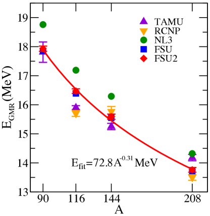
Figure 1: (Color online) Constrained giant monopole energies for ⁹⁰Zr, ¹¹⁶Sn, ¹⁴⁴Sm, and ²⁰⁸Pb. Experimental data were obtained from experiments carried out at TAMU Youngblood et al. (1999) and RCNP Uchida et al. (2004); Li et al. (2007, 2010); Patel et al. (2013); Patel and Garg . Theoretical predictions are presented for NL3 Lalazissis et al. (1997), FSUGold Todd-Rutel and Piekarewicz (2005), and FSUGold 2 supplemented with theoretical errors. The red solid line represents a best fit to the FSUGold 2 predictions of the form $E_{\rm fit}\!=\!72.8A^{-0.31}$ MeV.

III.4 Neutron Star Structure

The last observable that was included in the calibration of the new FSU 2 functional was the maximum neutron star mass. Displayed in Fig. 2 with horizontal bars are the two most massive, and accurately measured, neutron stars observed to date Demorest et al. (2010); Antoniadis et al. (2013). Clearly, those observations place stringent constraints on the high-density component of the EOS, as models that predict limiting masses below $2\,M_{\odot}$—such as FSUGold—must be stiffened accordingly. Therefore, for the optimization of the FSU 2 functional, we have adopted a value of $M_{\rm max}\!=\!2.10\,M_{\odot}$ with a relatively small 1$\%$ error. If an even larger mass is discovered in the future, such new input can be easily incorporated into the calibration procedure.

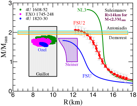
Figure 2: (Color online) Mass-vs-radius relation predicted by the three models considered in the text: NL3 Lalazissis et al. (1997), FSUGold Todd-Rutel and Piekarewicz (2005), and FSUGold 2. Also shown are recent observational constraints on neutron star masses Demorest et al. (2010); Antoniadis et al. (2013) and radii Ozel et al. (2010); Steiner et al. (2010); Suleimanov et al. (2011); Guillot et al. (2013). The FSUGold 2 results are supplemented with two sets of theoretical errors: one (red) in which the maximum neutron star mass was included in the calibration of the functional and the other (grey) estimated also using FSUGold 2, but with the impact of the maximum neutron star mass removed from the curvature matrix, as explained in the text.

Also displayed in Fig. 2 are theoretical predictions for the mass-vs-radius (M-R) relations for the three models considered in the text. As alluded earlier, with a stiff EOS, NL3 predicts large stellar radii and a maximum neutron star mass of almost $3\,M_{\odot}$. In contrast, FSUGold with a relatively soft EOS predicts smaller values for both. The new FSUGold 2 functional displays a M-R relation that appears intermediate between NL3 and FSUGold. In particular, after the optimization we obtain a maximum stellar mass of $M_{\rm max}\!=\!(2.07\!\pm 0.02)\,M_{\odot}$, safely within the bounds set by observation. Given the large impact that the quartic vector coupling constant $\zeta$ has on the EOS at high densities, these results are totally consistent with our expectations (see Table 1). On the other hand, stellar radii seem to be controlled by the density dependence of the symmetry energy in the immediate vicinity of saturation density Lattimer and Prakash (2007). Thus models with large values of $L$ tend to predict neutron stars with large radii Horowitz and Piekarewicz (2001b). This is the main reason behind the relatively uniform “shift” between FSU and FSU 2 (see Table 4.) It is important to realize that no observable highly sensitive to the density dependence of the symmetry energy, such as the neutron-skin thickness of ²⁰⁸Pb or stellar radii, was used in the calibration of FSU 2. Such a choice was deliberate, as at present there are no stringent experimental or observational constraints on the isovector sector of the nuclear density functional. Although the Lead Radius Experiment (“PREX”) at the Jefferson Laboratory has provided the first model-independent evidence on the existence of a neutron-rich skin in ²⁰⁸Pb Abrahamyan et al. (2012); Horowitz et al. (2012), the determination came with an error that is too large to impose any significant constraint. That is,

$$R_{\rm skin}^{208}\!=\!{0.33}^{+0.16}_{-0.18}\,{\rm fm}\,.$$ (18)

In the case of stellar radii, the present situation is highly unsatisfactory as further illustrated in Fig. 2. First, an initial attempt by Özel and collaborators to determine simultaneously the mass and radius of three x-ray bursters resulted in predictions for stellar radii between $8$ and $\!10$ km Ozel et al. (2010). Shortly after, Steiner et al. supplemented Özel’s study with three additional neutron stars and concluded that systematic uncertainties make the most probable radii lie in the 11-12 km region Steiner et al. (2010). However, even this more conservative estimate has been put into question by Suleimanov and collaborators, who suggested a lower limit on the stellar radius of 14 km on neutron stars with masses below $2.3\,M_{\odot}$ Suleimanov et al. (2011). That is, three different analyses of (mostly) the same sources seem to differ in their conclusions by more than 5 km in the radius of a typical neutron star. Recognizing this unfortunate situation and the many challenges posed by the study of x-ray bursters, Guillot and collaborators concentrated on the determination of stellar radii by studying five quiescent low mass x-ray binaries (qLMXB) in globular clusters. By clearly and explicitly stating all their assumptions, some of them apparently not without controversy Lattimer and Steiner (2013), Guillot et al. were able to determine a rather small neutron star radius of Guillot et al. (2013):

$$R_{0}=9.1^{+1.3}_{-1.5}\,{\rm km}\,.$$ (19)

Note that this value represents the “common” radius of all neutron stars, a critical assumption in the analysis of Ref. Guillot et al. (2013). Based on such a confusing state of affairs concerning stellar radii, we have then decided against including such information into the calibration of FSUGold 2.

Of course, this does not prevent us from offering FSU 2 predictions for stellar radii, as displayed in Fig. 2. In particular, we find the radius of a “canonical” $1.4\,M_{\odot}$ neutron star to be $R_{1.4}\!=\!(14.42\pm 0.26)\,{\rm km}$. Note that the large stellar radii predicted by FSU 2 satisfy the constraint set by Suleimanov et al., but only for neutron stars with masses below $\simeq\!1.8\,M_{\odot}$. Moreover, we should mention that although no assumptions on either the neutron-skin thickness of ²⁰⁸Pb or stellar radii were incorporated into the calibration of FSUGold 2, a manuscript that contemplates various possible scenarios is in preparation.

We close this section by exploring the impact of the maximum neutron star mass $M_{\rm max}$ on the estimation of errors. Recall that $M_{\rm max}$ is the only observable included in the calibration that is sensitive to the high-density component of the EOS. Although we preserve the same optimal set of parameters as FSUGold 2, we assess the impact of $M_{\rm max}$ by removing its contribution to the curvature matrix. This invariably results in some flattening of certain directions in parameter space. In particular, the additional set of theoretical errors displayed (in grey) in Fig. 2 were estimated in precisely this manner. As expected, the (grey) theoretical “error band” becomes significantly thicker when the maximum neutron star mass is removed from consideration. Particularly, the uncertainty in $M_{\rm max}$ is increased significantly from 0.02 to 0.15 $M_{\odot}$ and the error in the radius of a 1.4 $M_{\odot}$ neutron star becomes almost three times as large. It is clear that the inclusion of $M_{\rm max}$ in the calibration of the functional is essential to constrain the high-density component of the EOS. Indeed, we believe that no terrestrial experiment can reliably constrain the EOS of neutron star matter.

III.5 Predictions and Correlations

With the exception of stellar radii, up until now we have concentrated on physical observables that were included in the calibration of the density functional. In the present section we shift our attention to genuine theoretical predictions of a variety of observables that were not incorporated into the fit. We start by displaying in Table 4 a few bulk properties of nuclear matter at saturation density. These properties are of critical importance in constraining the EOS of neutron-rich matter and the covariance analysis developed here serves to determine whether the physical observables incorporated into the fit impose meaningful constraints on these properties. We note that the four isoscalar properties that characterize the EOS of SNM (i.e., $\rho_{\raisebox{-0.75pt}{\tiny 0}}$, $\varepsilon_{\raisebox{-0.75pt}{\tiny 0}}$, $M^{\ast}/M$, and $K$) are all accurately determined (to about 1%). In particular, we attribute the small theoretical error associated with the incompressibility coefficient ($K\!=\!238.0\pm 2.8$ MeV) to the inclusion of GMR energies into the calibration of FSUGold 2. Moreover, we find good agreement with the isoscalar predictions from both NL3 and FSU except in the case of $K$ for NL3.

​​Model	$\rho_{\raisebox{-0.75pt}{\tiny 0}}({\rm fm}^{-3})$	$\varepsilon_{\raisebox{-0.75pt}{\tiny 0}}\,{\rm(MeV)}$	$M^{\ast}\!/M$	$K\,{\rm(MeV)}$	$J\,{\rm(MeV)}$	$L\,{\rm(MeV)}$
​​NL3	0.1481	$-$16.24	0.595	271.5	37.28	118.2
FSU	0.1484	$-$16.30	0.610	230.0	32.59	060.5
FSU 2	$0.1505\pm 0.0007$	$-16.28\pm 0.02$	$0.593\pm 0.004$	$238.0\pm 2.8$	$37.62\pm 1.11$	$112.8\pm 16.1$

Table 4: Bulk properties of nuclear matter as predicted by the three models considered in the text: NL3 Lalazissis et al. (1997), FSUGold Todd-Rutel and Piekarewicz (2005), and FSUGold 2 supplemented with theoretical errors.

However, the situation is radically different in the isovector sector. Although the ground-state properties of neutron-rich nuclei, such as ⁴⁸Ca, ¹³²Sn, ²⁰⁸Pb, are able to constrain the value of the symmetry energy $J$ to about 3%, its slope $L$ remains poorly constrained (to about 15%). We attribute this situation to the lack of well measured isovector observables, such as the neutron skin of heavy nuclei. We reiterate that when relativistic models of the kind given in Eq. (1) do not incorporate strong isovector constraints, they tend to generate a fairly stiff symmetry energy. However, note that although the density dependence of the symmetry energy remains rather uncertain, all three models considered in the table seem to agree on its value at a sub-saturation density of $\widetilde{\rho_{\raisebox{-0.75pt}{\tiny 0}}}\!\approx\!0.10\,{\rm fm}^{-3}\!\approx\!2\rho_{\raisebox{-0.75pt}{\tiny 0}}/3$. Indeed, according to Eq. (4b) one obtains

$$\tilde{J}\equiv{\cal S}(\widetilde{\rho_{\raisebox{-0.75pt}{\tiny 0}}})\approx J+L\frac{(\widetilde{\rho_{\raisebox{-0.75pt}{\tiny 0}}}\!-\!\rho_{\raisebox{-0.75pt}{\tiny 0}})}{3\rho_{\raisebox{-0.75pt}{\tiny 0}}}\approx\left(J\!-\!\frac{L}{9}\right)\approx(25\!-\!26)\,{\rm MeV}\,.$$ (20)

This point has been emphasized repeatedly in various references Farine et al. (1978); Brown (2000); Horowitz and Piekarewicz (2001a); Furnstahl (2002); Zhang and Chen (2013); Brown (2013); Horowitz et al. (2014). That is, the above correlation between $J$ and $L$ that emerges from the masses of neutron-rich nuclei determines rather accurately the value of the symmetry energy at an average between the central nuclear density $\rho_{\raisebox{-0.75pt}{\tiny 0}}$ and some characteristic density at the surface. Clearly, more information is required to determine uniquely both $J$ and $L$.

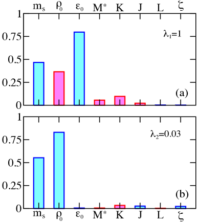
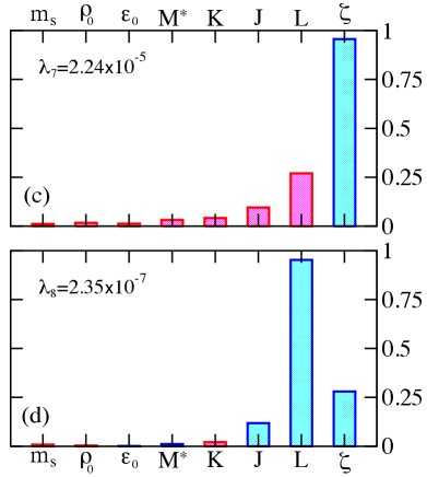
Figure 3: (Color online) Amplitude decomposition of the eigenvectors of the curvature matrix corresponding to the two largest [(a) and (b)] and the two smallest [(c) and (d)] eigenvalues, with the largest eigenvalue normalized to one. The two different colors (blue and red) indicate that the amplitudes contribute with opposite signs.

The large theoretical error attached to the prediction of $L$ suggests that relatively large changes in $L$ from its average value produce a mild deterioration in the quality of the fit. This indicates that there are directions in the model space that are relatively “soft” or “flat”. A highly intuitive way to illustrate this effect is to diagonalize the $8\!\times\!8$ curvature matrix $\hat{\cal M}$ defined in Eq. (13), which then becomes effectively a small-oscillations problem. In particular, each eigenvalue $\lambda_{i}$ of $\hat{\cal M}$ controls the deterioration in the quality of the fit as one moves along a direction defined by its corresponding eigenvector Fattoyev and Piekarewicz (2011). A “flat” direction, characterized by a small eigenvalue $\lambda_{i}$, involves a particular linear combination of parameters that is poorly constrained by the choice of observables included in the calibration of the functional. We depict such a behavior in Fig. 3 by displaying the components of four of the eigenvectors along the original directions in the pseudo-parameter space. Note that we have considered only those eigenvectors having the two largest and two smallest eigenvalues, with the largest eigenvalue being normalized arbitrarily to one. The blue and red rectangles serve to indicate component having opposite signs. The eigenvectors associated with the two largest eigenvalues determine the two stiffest directions in parameter space. Small departures from the minimum along those two eigenvectors result in a rapid deterioration of the quality of the fit. Perhaps not surprisingly given the importance of ground-state energies and charge radii (see Table 2), the scalar-meson mass, the saturation density, and the binding energy per nucleon are the most accurately determined parameters. Note that the scalar mass was determined with a small 0.3% theoretical error: $m_{\rm s}\!=\!(497.479\pm 1.492)\,{\rm MeV}$. In stark contrast, the eigenvalues associated with the two softest directions are down by five to seven orders of magnitude. These two directions are represented by almost “pure” eigenvectors with amplitudes in excess of 0.95 along the original $\zeta$ and $L$ directions, respectively. The reason for $L$ to remain poorly constrained has already been discussed earlier. However, the reason for $\zeta$ to remain largely undetermined is slightly more subtle. From the work of Müller and Serot it is already known that the value of $\zeta$ is insensitive to ground-state properties of finite nuclei that probe densities near nuclear matter saturation Mueller and Serot (1996). On the other hand, Müller and Serot showed that the value of $\zeta$ may be efficiently tuned to control the high-density component of the EOS, and ultimately the maximum neutron star mass $M_{\rm max}$. Naively then, one would have expected a better constraint on $\zeta$ from the inclusion of $M_{\rm max}$ in the calibration of the functional. We believe that the poor determination of $\zeta$ may be attributed to the large value of $L$ suggested by FSUGold 2 (see Table 4). Indeed, when $L$ is small as in the case of FSUGold, the high-density component of the EOS needs to be stiffened to account for the existence of massive stars. And this can be efficiently done by only tuning $\zeta$, as was done in Ref. Fattoyev et al. (2010). However, if the symmetry energy is already stiff and no isovector constraints are available, then it appears that only a linear combination of $L$ and $\zeta$ can be constrained. This analysis reinforces the urgent need for well measured isovector observables.

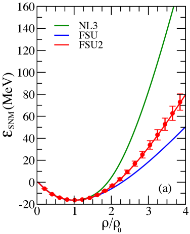
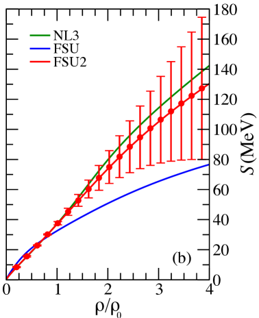
Figure 4: (Color online) (a) Binding energy per nucleon of symmetric nuclear matter and (b) symmetry energy as a function of density in units of nuclear matter saturation density $\rho_{{}_{0}}\!=0.148\,{\rm fm}^{-3}$. Predictions are included from the three models discussed in the text: NL3 Lalazissis et al. (1997), FSUGold Todd-Rutel and Piekarewicz (2005), and FSUGold 2 supplemented with theoretical errors.

A more detailed view of the behavior of infinite nuclear matter is given in Fig. 4 where predictions for the EOS of SNM (left panel) and the symmetry energy (right panel) are displayed for the three RMF models considered in this work. Due to the inclusion of GMR energies into the calibration of FSUGold 2, the incompressibility coefficient was fairly accurately determined (see Table 4) and this, in turn, generates small theoretical errors on the EOS up to 2-3 times saturation density. The larger theoretical uncertainty with increasing density is a reflection of the inability of ground-state properties and GMR energies to constrain the high-density behavior of the EOS. In principle, the inclusion of a maximum neutron star mass $M_{\rm max}$ into the fit should have served to constrain the EOS at high density. However, given that the symmetry energy is stiff (see right-hand panel) one can satisfy the $M_{\rm max}$ constraint without imposing stringent limits on the EOS of SNM at high densities. The situation appears to be radically different in the case of the symmetry energy, as the model has lost its predicability at densities only slightly above saturation density. Although we expect to mitigate this situation once strong isovector observables, such as neutron skins and stellar radii, are incorporated into the calibration of the density functional, our results underscore the importance of including theoretical uncertainties. Whereas the symmetry energy predicted by FSUGold 2 is stiff at saturation density, it is consistent at the 1$\sigma$ level with a symmetry energy almost as soft as FSUGold and as stiff as (or even stiffer than) NL3 at high densities. The impact of a stiff symmetry energy on the neutron-skin thickness of all the nuclei used in the calibration procedure is displayed in Table 5. These results help to reinforce the recent claim that at present there is no compelling reason to rule out models with large neutron skins Fattoyev and Piekarewicz (2013). We close this part of the discussion with a brief comment on the EOS of pure neutron matter. Given that the EOS of PNM may be approximated as that of SNM plus the symmetry energy, the EOS of PNM at low densities for FSUGold 2 strongly resembles the one for NL3. Although PNM is not experimentally accessible, there are important theoretical constraints that have emerged from the universal behavior of dilute Fermi gases in the unitary limit Schwenk and Pethick (2005). As already mentioned, without additional isovector constraints the symmetry energy predicted by RMF models tends to be fairly stiff. Therefore, whereas FSUGold is consistent with most theoretical constraints Schwenk and Pethick (2005); Gezerlis and Carlson (2008, 2010); Vidana et al. (2009), both FSUGold 2 and NL3 are not.

​​Nucleus	NL3	FSU	FSU 2
​​16O	$-0.028$	$-0.029$	$-0.028\pm 0.005$
40Ca	$-0.049$	$-0.051$	$-0.050\pm 0.004$
48Ca	0.226	0.197	$0.232\pm 0.008$
68Ni	0.261	0.211	$0.268\pm 0.010$
90Zr	0.114	0.088	$0.117\pm 0.008$
100Sn	$-0.076$	$-0.080$	$-0.077\pm 0.008$
116Sn	0.167	0.122	$0.172\pm 0.011$
132Sn	0.346	0.271	$0.354\pm 0.019$
144Sm	0.145	0.103	$0.149\pm 0.011$
208Pb	0.278	0.207	$0.287\pm 0.020$

Table 5: Predictions for the neutron skins, $R_{\rm skin}\!\equiv\!R_{\rm n}\!-\!R_{\rm p}$, (in fm) of all the nuclei included in the calibration procedure for NL3 Lalazissis et al. (1997), FSUGold Todd-Rutel and Piekarewicz (2005), and FSUGold 2 supplemented with theoretical error bars.

So far we have discussed the results from the optimization and the theoretical errors associated to a large number of physical quantities. We now turn the discussion to the important topic of correlations [see Eqs. (14) and (15)]. We start in Fig. 5 by displaying correlation coefficients in graphical form for various physical quantities. From these, only GMR energies and the maximum neutron star mass were included in the calibration procedure. As anticipated, we find a strong correlation of the GMR energies to the nuclear incompressibility coefficient $K$, verifying the age-old idea of extracting a fundamental parameter of the EOS from laboratory measurements of the breathing mode. To our knowledge, this is the first time that GMR energies are directly incorporated into the calibration of a relativistic EDF. In the case of the two fundamental parameters of the symmetry energy $J$ and $L$, we observe a strong correlation with “size” parameters, specifically with the neutron radius of ⁴⁸Ca and ²⁰⁸Pb, as well as with the radius of “canonical” 1.4 $M_{\odot}$ neutron star. The sensitivity of the size parameters to $L$ has a clear physical underpinning. In the particular case of a nucleus, surface tension favors the formation of a spherical drop of uniform equilibrium density. However, if the nucleus has a significant neutron excess, it may be energetically advantageous to move some of these neutrons from the center of the nucleus to the dilute surface where the symmetry energy is reduced. In particular, if the slope $L$ is large, then this reduction is significant so it becomes favorable to move most of the excess neutrons to the surface, thereby creating a thick neutron skin Horowitz et al. (2014). And given that the same pressure that pushes against surface tension in a nucleus pushes against gravity in a neutron star, the larger the value of $L$ the larger the stellar radius Horowitz and Piekarewicz (2001a, b). However, whereas the neutron skin is sensitive to the pressure around the saturation density, the neutron star radius also depends on the pressure at higher densities. This weakens slightly the correlation between the stellar radius and the neutron radius of the nucleus. Nevertheless, that a correlation between systems that differ in size by 18 orders of magnitude exists, is remarkable indeed. Moreover, the correlation between the neutron-skin thickness of ²⁰⁸Pb and the radius of low mass neutron stars is even stronger Carriere et al. (2003); Fattoyev and Piekarewicz (2012). This suggests how a laboratory measurement may place a significant constraint on an astronomical object, and vice versa. This example clearly illustrates the power of the covariance analysis.

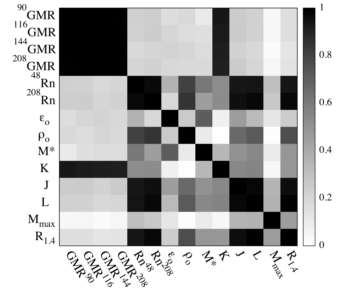
Figure 5: Correlation coefficients (in absolute value) depicted in graphical form for a representative set of observables. The set includes four GMR energies (for ⁹⁰Zr, ¹¹⁶Sn, ¹⁴⁴Sm, and ²⁰⁸Pb), two neutron radii (for ⁴⁸Ca and ²⁰⁸Pb), several bulk properties of nuclear matter ($\varepsilon_{{}_{0}}$, $\rho_{{}_{0}}$, $M^{\ast}$, $K$, $J$, and $L$), and two neutron star observables (the maximum mass $M_{\rm max}$ and the radius of a 1.4 $M_{\odot}$ neutron star $R_{1.4}$).

We now proceed to display in Fig. 6 correlation coefficients between the Lagrangian model parameters. The prevalence of “dark patches” suggests a strong correlation among several model parameters. A large correlation coefficient of $\big{|}\rho(A,B)\big{|}\simeq\!1$ between two observables may indicate “redundancy”, in the sense that there may be little to gain by including both observables in the calibration procedure. This could alleviate the need for performing a complex experiment. Alternatively, a strong correlation may suggest an experiment that could constrain the value of an inaccessible quantity. However, in the case of the model parameters, a strong correlation does not imply redundancy, but quite the opposite. For example, a strong correlation between two well determined model parameters, such as $g_{\rm s}^{2}\!=\!108.0943\pm 1.8376$ and $g_{\rm v}^{2}\!=\!183.7893\pm 4.9623$ implies a strong interdependence. That is, if $g_{\rm s}^{2}$ is fixed at a certain value, then $g_{\rm v}^{2}$ must attain the precise value suggested by their correlation; otherwise the quality of the fit will deteriorate significantly.

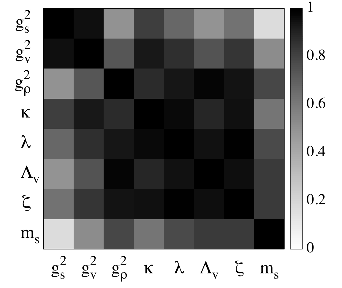
Figure 6: Correlation coefficients (absolute values) between Lagrangian model parameters depicted in graphical form.

We conclude by displaying in Fig. 7 correlation coefficients between the Lagrangian model parameters and a representative set of physical observables. Contrary to expectations, the strong correlation between $\zeta$ and the maximum neutron star mass is missing. As already explained, a large maximum neutron star mass may be generated by having either a stiff EOS for SNM or a stiff symmetry energy. If the symmetry energy is soft, as in the case of FSUGold, then one must stiffen the EOS of SNM, which may be efficiently done by tuning $\zeta$. However, given that the symmetry energy predicted by FSUGold 2 is stiff (see Fig. 4) the correlation between $\zeta$ and $M_{\rm max}$ weakens. Indeed, $M_{\rm max}$ displays the strongest correlation with the two isovector parameters $g_{\rho}^{2}$ and $\Lambda_{\rm v}$—although the correlation is fairly weak. This suggests that the maximum mass constraint results from a competition between $\zeta$ and the slope of symmetry energy $L$. For instance, if $\zeta$ increases, thereby softening the EOS of SNM, then $M_{\rm max}$ is reduced. Thus, in order to maintain $M_{\rm max}$ at its specified value, the symmetry energy must stiffen accordingly. This implies a strong and positive correlation between $\zeta$ and $L$, as precisely indicated in Fig. 7. An important lesson learned from the present discussion is that one must exercise caution in examining correlations among parameters and observables. For example, it appears that certain bulk parameters of SNM, such as the binding energy per nucleon $\varepsilon_{\raisebox{-0.75pt}{\tiny 0}}$, the effective nucleon mass $M^{\ast}$, and the incompressibility coefficient $K$ are uncorrelated to the four isoscalar parameters $g_{\rm s}^{2}$, $g_{\rm v}^{2}$, $\kappa$, and $\lambda$. Such lack of correlation may come as a surprise in view that $\varepsilon_{\raisebox{-0.75pt}{\tiny 0}}$, $M^{\ast}$, $K$, and the saturation density $\rho_{\raisebox{-0.75pt}{\tiny 0}}$ uniquely determine the value of the four isoscalar parameters (see appendix). The solution to this apparent contradiction lies in the fact that in generating the distribution of Lagrangian model parameters all four isoscalar parameters become inextricably linked. In order to isolate the proper correlation between a given observables (say $\varepsilon_{\raisebox{-0.75pt}{\tiny 0}}$) and a given model parameter (say $g_{\rm s}^{2}$) one should monitor the response of the observable to changes to only that one parameter. That is, if one could provide suitable selection cuts to maintain the other parameters (say $g_{\rm v}^{2}$, $\kappa$, and $\lambda$) fixed, then the strong correlation between $\varepsilon_{\raisebox{-0.75pt}{\tiny 0}}$ and $g_{\rm s}^{2}$ will become manifest Piekarewicz et al. (2014).

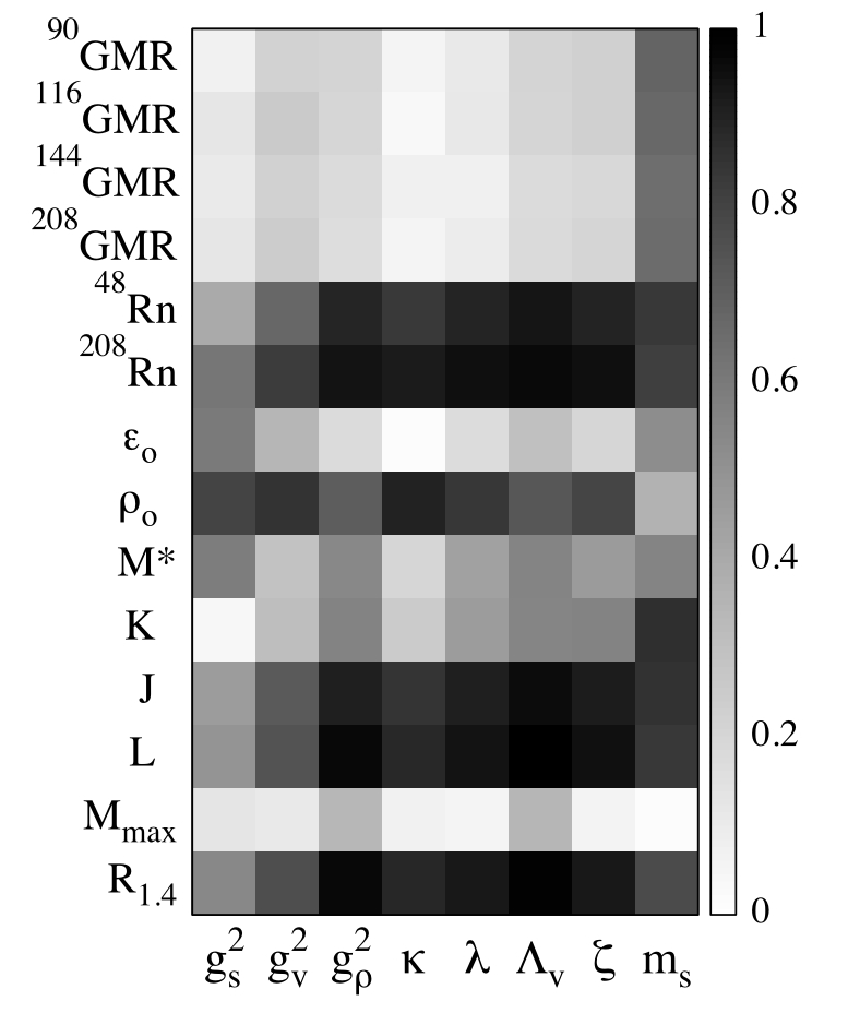
Figure 7: Correlation coefficients (absolute values) between Lagrangian model parameters and a representative set of physical observables. The set of observables are the same as those considered in Fig. 5.

IV Summary and Outlook

Finite nuclei, infinite nuclear matter, and neutron stars are strongly interacting, nuclear many-body systems that span an enormous range of densities and isospin asymmetries. Lacking the tools to solve QCD in these regimes, DFT-based approaches, such as Skyrme and RMF models, provide the most powerful alternative for investigating such complex systems within a single unified framework. For the systematic study of such diverse nuclear systems, we have developed a new RMF model, FSUGold 2, to describe the physics of both finite nuclei and neutron stars; objects that differ in size by 18 orders of magnitude.

The philosophy behind our calibration procedure adheres to two guiding principles. First, the calibration relies exclusively on genuine physical observables that can be measured either in the laboratory or extracted from observation. Second, the optimization of the functional was implemented in the space of “pseudo data”, consisting mostly of bulk properties of infinite nuclear matter. This has the enormous advantage that, unlike the Lagrangian model parameters, the pseudo data have both a clear physical interpretation and acceptable values that range over a fairly narrow interval. To our knowledge, this is the first time that such a transformation between model parameters and pseudo data is implemented in the relativistic domain. We should note that in an effort to limit the input to only accurately measured physical observables, neither neutron skins of neutron-rich nuclei nor radii of neutron stars were included in the optimization. Hence, values for these observables become bona-fide model predictions.

In addition to neutron skins and stellar radii, we provide predictions for a variety of bulk properties of both symmetric nuclear matter and the symmetry energy. Isoscalar properties, such as the density, binding energy per nucleon, and incompressibility coefficient of SNM at saturation are all determined with small theoretical errors and in close agreement with their conventionally accepted values. In particular, the incompressibility coefficient was determined with a theoretical uncertainty of only 1%. Such a small theoretical error was obtained by the inclusion of GMR energies into the calibration of FSUGold 2. This too, we believe, has been done here for the first time. The theoretical errors attached to the predictions of $\rho_{\raisebox{-0.75pt}{\tiny 0}}$ and $\varepsilon_{\raisebox{-0.75pt}{\tiny 0}}$ are even smaller, indicating that the isoscalar sector is well constrained by the binding energies, charge radii, and GMR energies of finite nuclei.

The lack of well measured isovector observables in the calibration of the functional has radically different consequences on the determination of the bulk parameters of the symmetry energy, especially in the case of its slope $L$. First, without stringent isovector constraints, RMF models of the type used here tend to favor a stiff symmetry energy. Indeed, we obtained a value for the slope of the symmetry energy of $L\!=\!(112.8\pm 16.1)\,{\rm MeV}$. In turn, this large slope yields values of $R_{\rm skin}^{208}\!=\!(0.287\pm 0.020)\,{\rm fm}$ and $R_{1.4}\!=\!(14.42\pm 0.26)\,{\rm km}$ for the neutron-skin thickness of ²⁰⁸Pb and the radius of a 1.4 $M_{\odot}$ neutron star, respectively. Although both large, we underscore that at present there is no conclusive experimental measurement nor astrophysical observation that can rule out large neutron skins Fattoyev and Piekarewicz (2013) or large stellar radii. Thus, there is urgent need for the accurate determination of both.

Following the optimization of the density functional, we proceeded to explore the richness of the covariance analysis. This we did in two stages. First, we provided predictions for a variety of observables with properly estimated theoretical errors. This is particularly critical when models are extrapolated to unknown regions. Second, we explored correlations between both observables and model parameters. A correlation analysis can reveal interdependences that may be of great value. For example, a strong correlation between two observables may eliminate the need to measure both. Further, if from these two observables, e.g., $L$ and $R_{\rm skin}^{208}$, one of these is of critical importance but inaccessible in the laboratory (e.g., $L$) one could measure the latter to determine the former. Although there are ambitious plans to experimentally constrain the isovector sector by improving and expanding on previous measurements of both neutron skins and electric dipole polarizabilities, we will use some of the insights developed here to anticipate several different outcomes. We are planning to exploit the power and flexibility of the covariance analysis to constrain the poorly determined isovector parameters $g_{\rho}^{2}$ and $\Lambda_{\rm v}$ by assuming a variety of scenarios involving neutron skins of neutron-rich nuclei. For example, how precisely does one have to measure the neutron radius of ²⁰⁸Pb in order to constrain $L$ to a given acceptable range? Is this precision attainable with PREX-II? If not, what other neutron-rich nuclei should be used? Or, is it better to measure the weak form factor of ²⁰⁸Pb at another momentum transfer? In this manner the development of an efficient modeling scheme is invaluable for the simulation of various scenarios. Research along these lines is in progress and its results will be presented in a forthcoming publication.

*

Appendix A

In this appendix we describe the connection between the coupling constants appearing in the Lagrangian density depicted in Eq. (1) and various bulk parameters of infinite nuclear matter. This connection has proved to be extremely useful. Indeed, expressing the objective function in terms of physically intuitive parameters provides important insights on the quest for the optimal parametrization. For example, based on the large experimental database of accurately measured nuclear masses, both the saturation density and the energy per nucleon at saturation are fairly well known. In turn, limiting the searches to a narrow region of parameter space increases significantly the efficiency of the Levenberg-Marquardt algorithm. We start by connecting the isoscalar sector of the Lagrangian density with a few bulk parameters of symmetric nuclear matter Glendenning (2000). We then proceed to determine the two isovector parameters of the Lagrangian density ($g_{\rho}^{2}$ and $\Lambda_{\rm v}$) from the value of the symmetry energy $J$ and its slope $L$ at saturation density. To our knowledge, we are the first ones to establish such a connection in the isovector sector.

A.1 Isoscalar sector

Given the Lagrangian density of Eq. (1), the energy density (${\mathscr{E}}\!=\!E/V$) of infinite nuclear matter may be computed directly from the corresponding energy-momentum tensor in the mean-field approximation. Note that only the zero-temperature limit will be addressed. Restricting ourselves to the isoscalar sector, the energy density of symmetric nuclear matter is given by the following expression Serot and Walecka (1986):

$${\mathscr{E}}(\rho) =\gamma\int_{0}^{k_{\rm F}}\frac{d^{3}k}{(2\pi)^{3}}E_{k}^{{}^{(+)}}+\left(\frac{1}{2}\frac{m_{\rm s}^{2}}{g_{\rm s}^{2}}\Phi_{0}^{2}+\frac{\kappa}{6}\Phi_{0}^{3}+\frac{\lambda}{24}\Phi_{0}^{4}\right)-\left(\frac{1}{2}\frac{m_{\rm v}^{2}}{g_{\rm v}^{2}}W_{0}^{2}+\frac{\zeta}{24}W_{0}^{4}\right)$$

$$=\frac{M^{\ast 4}}{4\pi^{2}}\left[\frac{k_{\rm F}E_{\rm F}^{\star}\left(k_{\rm F}^{2}+E_{\rm F}^{\star 2}\right)}{M^{\ast 4}}\!-\!\ln\left(\frac{k_{\rm F}+E_{\rm F}^{\star}}{M^{\ast}}\right)\right]+\left(\frac{1}{2}\frac{m_{\rm s}^{2}}{g_{\rm s}^{2}}\Phi_{0}^{2}+\frac{\kappa}{6}\Phi_{0}^{3}+\frac{\lambda}{24}\Phi_{0}^{4}\right)+\left(\rho_{\rm v}W_{0}-\frac{1}{2}\frac{m_{\rm v}^{2}}{g_{\rm v}^{2}}W_{0}^{2}-\frac{\zeta}{24}W_{0}^{4}\right)\,.$$ (21)

where $\gamma\!=\!4$ is the spin-isospin degeneracy, $\rho_{\rm v}\!\equiv\!\rho=(2k_{\rm F}^{3})/(3\pi^{2})$ is the conserved baryon density, $\Phi_{0}\!=g_{\rm s}\phi_{0}$, $W_{0}\!=g_{\rm v}V_{0}$, $M^{\ast}\!=\!M\!-\!\Phi_{0}$ is the effective nucleon mass, and $E_{k}^{{}^{(+)}}\!=\!E_{k}^{\ast}+W_{0}\!=\!\sqrt{k^{2}\!+\!M^{\ast 2}}+W_{0}$ is the single-nucleon energy. Note that the classical equations of motion for the meson fields may be obtained directly from the Lagrangian density or equivalently, by demanding that the derivatives of ${\mathscr{E}}(\rho)$ with respect to $\Phi_{0}$ and $W_{0}$ both vanish. That is,

$$\frac{\partial{\mathscr{E}}}{\partial\Phi_{0}}=\frac{m_{\rm s}^{2}}{g_{\rm s}^{2}}\Phi_{0}+\frac{\kappa}{2}\Phi_{0}^{2}+\frac{\lambda}{6}\Phi_{0}^{3}-\rho_{\rm s}=0\,\,,$$ (22a)

$$\frac{\partial{\mathscr{E}}}{\partial W_{0}}=\frac{m_{\rm v}^{2}}{g_{\rm v}^{2}}W_{0}+\frac{\zeta}{6}W_{0}^{3}-\rho_{\rm v}=0\,.$$ (22b)

Here $\rho_{\rm s}$ is the scalar density that is defined as follows:

$$\rho_{\rm s}(M^{\ast})=\gamma\int_{0}^{k_{\rm F}}\frac{d^{3}k}{(2\pi)^{3}}\frac{M^{\ast}}{E_{k}^{\star}}=\frac{M^{\ast 3}}{\pi^{2}}\left[\frac{k_{\rm F}E_{\rm F}^{\star}}{M^{\ast 2}}-\ln\left(\frac{k_{\rm F}+E_{\rm F}^{\star}}{M^{\ast}}\right)\right]\,.$$ (23)

Note that the scalar density is not conserved and must be self-consistently determined from the equations of motion.

At zero temperature the pressure of the system may be calculated from its thermodynamic definition, i.e.,

$$P=-\left(\frac{\partial E}{\partial V}\right)_{\!N}=\rho\frac{\partial{\mathscr{E}}}{\partial\rho}-{\mathscr{E}}=\rho\left(E_{\rm F}^{{}^{(+)}}-\frac{E}{A}\right)\,,$$ (24)

where the last line follows from using $\partial{\mathscr{E}}/{\partial\rho}\!=\!E_{\rm F}^{{}^{(+)}}$, an identity that should hold in any thermodynamically consistent many-body theory. Moreover, note that at saturation density, the pressure vanishes and one obtains—in accordance with the Hugenholtz-van Hove theorem—that the energy per nucleon becomes equal to the Fermi energy. That is,

$$E_{\rm F}^{{}^{(+)}}=\sqrt{k_{\rm F}^{2}+M^{\ast 2}}+W_{0}=\frac{E}{A}\,.$$ (25)

To make further progress, we now obtain an analytic expression for the incompressibility coefficient of symmetric nuclear matter $K$. As defined in Eq. (4a), it is given by

$$K=9\rho_{\raisebox{-0.75pt}{\tiny 0}}^{2}\left[\frac{d^{2}(E/A)}{d\rho^{2}}\right]_{\!0}=9\rho_{\raisebox{-0.75pt}{\tiny 0}}^{2}\left[\frac{d}{d\rho}\!\left(\frac{P}{\rho^{2}}\right)\right]_{\!0}=9\rho_{\raisebox{-0.75pt}{\tiny 0}}\!\left(\frac{dE_{\rm F}^{{}^{(+)}}}{d\rho}\right)_{\!\!0}\,.$$ (26)

Given that the Fermi energy depends in a complicated way on the density, i.e., both explicitly and implicitly through $M^{\ast}$ and $W_{0}$, there are three terms that need to be evaluated. That is,

$$\frac{K}{9\rho_{\raisebox{-0.75pt}{\tiny 0}}}= \left(\frac{\partial E_{\rm F}^{{}^{(+)}}}{\partial\rho}\right)_{\!\!0}+\left(\frac{\partial E_{\rm F}^{{}^{(+)}}}{\partial W_{0}}\right)_{\!\!0}\!\left(\frac{{\partial W_{0}}}{\partial\rho}\right)_{\!\!0}+\left(\frac{\partial E_{\rm F}^{{}^{(+)}}}{\partial M^{\ast}}\right)_{\!\!0}\!\left(\frac{{\partial M^{\ast}}}{\partial\rho}\right)_{\!\!0}$$

$$= \left(\frac{\partial E_{\rm F}^{{}^{(+)}}}{\partial\rho}\right)_{\!\!0}+\left(\frac{{\partial W_{0}}}{\partial\rho}\right)_{\!\!0}+\left(\frac{M^{\ast}}{E_{\rm F}^{\ast}}\right)_{\!\!0}\!\left(\frac{{\partial M^{\ast}}}{\partial\rho}\right)_{\!\!0}\,.$$ (27)

We now proceed to evaluate each of the three terms. The first one is the simplest and yields:

$$\left(\frac{\partial E_{\rm F}^{{}^{(+)}}}{\partial\rho}\right)_{\!\!0}=\left(\frac{\pi^{2}}{2k_{\rm F}E_{\rm F}^{\ast}}\right)_{\!\!0}\,.$$ (28)

We continue with the second term and make use of the equation of motion for $W_{0}$ [Eq. (22b)] to write:

$$\left(\frac{{\partial W_{0}}}{\partial\rho}\right)_{\!\!0}=\left(\frac{g_{\rm v}^{2}}{m_{\rm v}^{\ast 2}}\right)_{\!\!0}\,,\hskip 5.69046pt{\rm with}\hskip 4.26773ptm_{\rm v}^{\ast 2}\equiv m_{\rm v}^{2}+\frac{\zeta}{2}g_{\rm v}^{2}W_{0}^{2}\,.$$ (29)

Using the previous two results we can rewrite Eq. (27) as follows:

$$\left(\frac{{\partial M^{\ast}}}{\partial\rho}\right)_{\!\!0}=\Bigg{[}\frac{E_{\rm F}^{\ast}}{M^{\ast}}\left(\frac{K}{9\rho}-\frac{\pi^{2}}{2k_{\rm F}E_{\rm F}^{\ast}}-\frac{g_{\rm v}^{2}}{m_{\rm v}^{\ast 2}}\right)\Bigg{]}_{\!0}\,.$$ (30)

The left-hand side of the equation may be computed by invoking the scalar equation of motion [Eq. (22a)] and depends on the three isoscalar coupling constants. We obtain,

$$\left(\frac{{\partial M^{\ast}}}{\partial\rho}\right)_{\!\!0}=-\Bigg{[}\frac{M^{\ast}}{E_{\rm F}^{\ast}}\left(\frac{m_{\rm s}^{\ast 2}}{g_{\rm s}^{2}}+\rho_{\rm s}^{\,\prime}(M^{\ast})\right)^{-1}\Bigg{]}_{\!0}\,,\hskip 5.69046pt{\rm with}\hskip 4.26773pt\frac{m_{\rm s}^{\ast 2}}{g_{\rm s}^{2}}\equiv\frac{m_{\rm s}^{2}}{g_{\rm s}^{2}}+\kappa\Phi_{0}+\frac{\lambda}{2}\Phi_{0}^{2}\,.$$ (31)

Note that we have defined the derivative of the scalar density [Eq. (23)] with respect to $M^{\ast}$ as follows:

$$\rho_{\rm s}^{\,\prime}(M^{\ast})=\left(\frac{\partial\rho_{\rm s}}{\partial M^{\ast}}\right)=\frac{1}{\pi^{2}}\left[\frac{k_{\rm F}}{E_{\rm F}^{\star}}(E_{\rm F}^{\star 2}+2M^{\ast 2})-3M^{\ast 2}\ln\left(\frac{k_{\rm F}+E_{\rm F}^{\star}}{M^{\ast}}\right)\right].$$ (32)

This is all the formalism that is needed to establish the connection between the isoscalar parameters appearing in the Lagrangian and a few bulk parameters of infinite nuclear matter. In the isoscalar sector the four bulk parameters of infinite nuclear matter that we consider here are as follows: (i) the density $\rho$, (ii) the binding energy per nucleon $E/A$, (iii) the incompressibility coefficient $K$, and (iv) the effective nucleon mass $M^{\ast}$—all of them evaluated at saturation density. Specification of these four bulk parameters enables one to determine four out of the five isoscalar coupling constants, namely, $g_{\rm v}^{2}/m_{\rm v}^{2}$, $g_{\rm s}^{2}/m_{\rm s}^{2}$, $\kappa$, and $\lambda$. The sole remaining coupling constant $\zeta$ is left intact as it is fairly insensitive to the properties of symmetric nuclear matter. Indeed, $\zeta$ is sensitive to the high-density component of the EOS and can be easily tuned by specifying the maximum neutron star mass. Note that in the mean-field approximation the Yukawa meson couplings always appear in combination with the corresponding meson mass.

The vector coupling may be readily determined from the vanishing of the pressure at saturation density. Indeed, from Eq. (25) one obtains the value of the vector field $W_{0}$ at saturation density. In turn, substituting this value in Eq. (22b) determines (for a given $\zeta$) $g_{\rm v}^{2}/m_{\rm v}^{2}$. Given that the vector mass has been fixed at its experimental value of $m_{\rm v}\!=\!782.5$ MeV, this provides a determination of $g_{\rm v}^{2}$.

The specification of the three isoscalar parameters is significantly more involved and depends critically on knowledge of the effective nucleon mass $M^{\ast}$ at saturation density. Further, it requires three independent pieces of information for their determination. Perhaps surprisingly, such information is provided in the form of three simultaneous linear equations. That is, the solution is unique. The first equation to be used involves the energy density of symmetric nuclear matter depicted in Eq. (21). Given that at saturation density ${\mathscr{E}}(\rho_{\raisebox{-0.75pt}{\tiny 0}})\!=\!\rho_{\raisebox{-0.75pt}{\tiny 0}}(E/A)_{0}$, every term in such expression is known—with the exception of $m_{\rm s}^{2}/g_{\rm s}^{2}$, $\kappa$, and $\lambda$. The classical equation of motion for the scalar field Eq. (22a) provides the second linear equation in these three parameters, since the scalar density is fully specified in terms of the density and effective nucleon mass at saturation. Finally, knowledge of the incompressibility coefficient $K$ at saturation density supplies the third and last linear equation. Indeed, a comparison between Eq. (30) and Eq. (31) indicates that the only unknown is the quantity $m_{\rm s}^{\ast 2}/g_{\rm s}^{2}$, which again contains the three scalar parameters of interest. Given that these equations provide a system of three simultaneous linear equations, the solution may be obtained by elementary means.

A.2 Isovector sector

In the previous section we concentrated on connecting the isoscalar parameters of the Lagrangian density to a few bulk parameters of symmetric nuclear matter. We now shift our focus to the isovector sector and show that the two isovector parameters $g_{\rho}^{2}/m_{\rho}^{2}$ and $\Lambda_{\rm v}$ may be determined from knowledge of two quantities of central importance, namely, the symmetry energy $J$ and its slope at saturation density $L$. To our knowledge, this connection is established here for the first time.

For the Lagrangian density given in Eq. (1), an analytic expression for the density dependence of the symmetry energy was derived in Ref. Horowitz and Piekarewicz (2001b). One obtains,

$$S(\rho)=\frac{k_{\rm F}^{2}}{6E_{\rm F}^{\star}}+\frac{g_{\rho}^{2}\rho}{8m_{\rho}^{\ast 2}}\,,\hskip 5.69046pt{\rm with}\hskip 4.26773pt\frac{m_{\rho}^{\ast 2}}{g_{\rho}^{2}}\equiv\frac{m_{\rho}^{2}}{g_{\rho}^{2}}+2\Lambda_{\rm v}W_{0}^{2}\,.$$ (33)

We note that the density dependence of the symmetry energy given above consists of a purely “isoscalar” term and a largely “isovector” term. That is, we define

$$S_{0}(\rho)\!=\!\frac{k_{\rm F}^{2}}{6E_{\rm F}^{\star}}\;\;{\rm and}\;\;S_{1}(\rho)\!=\!\frac{g_{\rho}^{2}\rho}{8m_{\rho}^{\ast 2}}\,.$$ (34)

In particular, given that the isoscalar sector has already been fixed, $S_{0}(\rho)$ along with all its derivatives are known. In contrast, $S_{1}(\rho)$ depends on both $g_{\rho}^{2}/m_{\rho}^{2}$ and $\Lambda_{\rm v}$ which are unknown. As already mentioned, critical to the determination of these two isovector parameters are the symmetry energy and its slope at saturation density, which according to Eq. (4b) are given as follows:

$$J=S(\rho_{\raisebox{-0.75pt}{\tiny 0}})\;\;{\rm and}\;\;L=3\rho_{\raisebox{-0.75pt}{\tiny 0}}\left(\frac{dS}{d\rho}\right)_{\!\!0}\,.$$ (35)

The determination of the quantity $m_{\rho}^{\ast 2}/g_{\rho}^{2}$, which still depends on both isovector parameters, is fairly simple:

$$J_{1}\equiv\left(\frac{g_{\rho}^{2}\rho}{8m_{\rho}^{\ast 2}}\right)_{\!\!0}=\Big{(}J\!-\!J_{0}\Big{)}=J-\left(\frac{k_{\rm F}^{2}}{6E_{\rm F}^{\star}}\right)_{\!\!0}\,.$$ (36)

In contrast, the determination of each individual isovector parameters is considerably more difficult and involves several of the same manipulations carried out in the isoscalar sector. In analogy with the above equation we write:

$$L_{1}=3\rho_{\raisebox{-0.75pt}{\tiny 0}}\!\left(\frac{dS_{1}}{d\rho}\right)_{\!\!0}=\Big{(}L\!-\!L_{0}\Big{)}=L-3\rho_{\raisebox{-0.75pt}{\tiny 0}}\!\left(\frac{dS_{0}}{d\rho}\right)_{\!\!0}\;.$$ (37)

We start by computing the contribution to the slope from the isoscalar term. That is,

$$L_{0} =3\rho_{\raisebox{-0.75pt}{\tiny 0}}\!\left(\frac{dS_{0}}{d\rho}\right)_{\!\!0}=3\rho_{\raisebox{-0.75pt}{\tiny 0}}\!\left[\left(\frac{\partial S_{0}}{\partial\rho}\right)+\left(\frac{\partial S_{0}}{\partial M^{\ast}}\right)\left(\frac{\partial M^{\ast}}{\partial\rho}\right)\right]_{0}$$

$$=J_{0}\Bigg{(}1+\frac{M^{\ast 2}}{E_{\rm F}^{\ast 2}}\left[1-\!\frac{3\rho}{\,M^{\ast}}\!\left(\frac{\partial M^{\ast}}{\partial\rho}\right)\right]\Bigg{)}_{\!0}\,.$$ (38)

Note that this expression is given exclusively in terms of isoscalar parameters, so it is completely known. Also note that the answer has been left in terms of $(\partial M^{\ast}\!/\partial\rho)_{{}_{0}}$ which has already been calculated in the previous section. We now proceed to compute the isovector contribution to the slope of the symmetry energy. Following similar steps as before, we obtain

$$L_{1} =3\rho_{\raisebox{-0.75pt}{\tiny 0}}\!\left(\frac{dS_{1}}{d\rho}\right)_{\!\!0}=3\rho_{\raisebox{-0.75pt}{\tiny 0}}\!\left[\left(\frac{\partial S_{1}}{\partial\rho}\right)+\left(\frac{\partial S_{1}}{\partial W_{0}}\right)\left(\frac{\partial W_{0}}{\partial\rho}\right)\right]_{0}$$

$$=3J_{1}\left[1-32\left(\frac{g_{\rm v}^{2}}{m_{\rm v}^{\ast 2}}\right)\!W_{0}\Lambda_{\rm v}J_{1}\right]_{0}=\Big{(}L\!-\!L_{0}\Big{)}\,.$$ (39)

This is all that is needed to achieve the desired goal of expressing $g_{\rho}^{2}/m_{\rho}^{2}$ and $\Lambda_{\rm v}$ in terms of $J$ and $L$. Indeed, given that $L$ is provided, and $J_{1}$ and $L_{0}$ have been determined from Eqs. (36) and (38), respectively, the only unknown in the previous equation is $\Lambda_{\rm v}$. Finally, using the definition of the effective $\rho$-meson mass given in Eq. (33), we can solve for $g_{\rho}^{2}/m_{\rho}^{2}$. That is,

$$\frac{m_{\rho}^{2}}{g_{\rho}^{2}}=\frac{m_{\rho}^{\ast 2}}{g_{\rho}^{2}}-2\Lambda_{\rm v}W_{0}^{2}=\frac{\rho_{\raisebox{-0.75pt}{\tiny 0}}}{8J_{1}}-2\Lambda_{\rm v}W_{0}^{2}\,.$$ (40)

References

- (1) “Building a universal nuclear energy density functional,” (UNEDF Collaboration).
- Kortelainen et al. (2010a) M. Kortelainen, T. Lesinski, J. More, W. Nazarewicz, J. Sarich, N. Schunck, M. V. Stoitsov, and S. Wild, Phys. Rev. C 82, 024313 (2010a).
- Kortelainen et al. (2012) M. Kortelainen, J. McDonnell, W. Nazarewicz, P.-G. Reinhard, J. Sarich, N. Schunck, M. V. Stoitsov, and S. M. Wild, Phys. Rev. C 85, 024304 (2012).
- Kortelainen et al. (2013) M. Kortelainen, J. McDonnell, W. Nazarewicz, E. Olsen, P.-G. Reinhard, J. Sarich, N. Schunck, S. M. Wild, D. Davesne, J. Erler, and A. Pastore, Phys. Rev. C 89, 054314 (2014).
- Walecka (1974) J. D. Walecka, Ann. Phys. (NY) 83, 491 (1974).
- Serot and Walecka (1986) B. D. Serot and J. D. Walecka, Adv. Nucl. Phys. 16, 1 (1986).
- Horowitz and Serot (1981) C. J. Horowitz and B. D. Serot, Nucl. Phys. A 368, 503 (1981).
- Lalazissis et al. (1997) G. A. Lalazissis, J. Konig, and P. Ring, Phys. Rev. C 55, 540 (1997) .
- Lalazissis et al. (1999) G. A. Lalazissis, S. Raman, and P. Ring, At. Data Nucl. Data Tables 71, 1 (1999).
- Todd-Rutel and Piekarewicz (2005) B. G. Todd-Rutel and J. Piekarewicz, Phys. Rev. Lett. 95, 122501 (2005) .
- Brown (2000) B. A. Brown, Phys. Rev. Lett. 85, 5296 (2000).
- Furnstahl (2002) R. J. Furnstahl, Nucl. Phys. A 706, 85 (2002) .
- Centelles et al. (2009) M. Centelles, X. Roca-Maza, X. Viñas, and M. Warda, Phys. Rev. Lett. 102, 122502 (2009) .
- Roca-Maza et al. (2011) X. Roca-Maza, M. Centelles, X. Vinas, and M. Warda, Phys. Rev. Lett. 106, 252501 (2011) .
- Erler et al. (2012) J. Erler, N. Birge, M. Kortelainen, W. Nazarewicz, E. Olsen, A. M. Perhac, and M. Stoitsov, Nature 486, 509 (2012).
- Afanasjev et al. (2013) A. V. Afanasjev, S. E. Agbemava, D. Ray, and P. Ring, Phys. Lett. B 726, 680 (2013).
- Lattimer and Prakash (2004) J. M. Lattimer and M. Prakash, Science 304, 536 (2004) .
- Demorest et al. (2010) P. Demorest, T. Pennucci, S. Ransom, M. Roberts, and J. Hessels, Nature 467, 1081 (2010) .
- Antoniadis et al. (2013) J. Antoniadis, P. C. Freire, N. Wex, T. M. Tauris, R. S. Lynch, et al., Science 340, 6131 (2013) .
- Editors (2011) The Editors, Phys. Rev. A 83, 040001 (2011).
- Reinhard and Nazarewicz (2010) P.-G. Reinhard and W. Nazarewicz, Phys. Rev. C 81, 051303 (2010) .
- Fattoyev and Piekarewicz (2011) F. J. Fattoyev and J. Piekarewicz, Phys. Rev. C 84, 064302 (2011) .
- Fattoyev and Piekarewicz (2012) F. J. Fattoyev and J. Piekarewicz, Phys. Rev. C 86, 015802 (2012) .
- Reinhard and Nazarewicz (2013) P.-G. Reinhard and W. Nazarewicz, Phys. Rev. C 87, 014324 (2013) .
- Reinhard et al. (2013) P.-G. Reinhard, J. Piekarewicz, W. Nazarewicz, B. Agrawal, N. Paar, et al., Phys. Rev. C 88, 034325 (2013) .
- Dobaczewski et al. (2014) J. Dobaczewski, W. Nazarewicz, and P.-G. Reinhard, J. Phys. G 41, 074001 (2014) .
- Piekarewicz et al. (2014) J. Piekarewicz, W.-C. Chen, and F. J. Fattoyev, arXiv:1407.0911 (2014) .
- Ozel et al. (2010) F. Ozel, G. Baym, and T. Guver, Phys. Rev. D 82, 101301 (2010) .
- Steiner et al. (2010) A. W. Steiner, J. M. Lattimer, and E. F. Brown, Astrophys. J. 722, 33 (2010) .
- Suleimanov et al. (2011) V. Suleimanov, J. Poutanen, M. Revnivtsev, and K. Werner, Astrophys. J. 742, 122 (2011) .
- Guillot et al. (2013) S. Guillot, M. Servillat, N. A. Webb, and R. E. Rutledge, Astrophys. J. 772, 7 (2013) .
- Schwenk and Pethick (2005) A. Schwenk and C. J. Pethick, Phys. Rev. Lett. 95, 160401 (2005) .
- Gezerlis and Carlson (2010) A. Gezerlis and J. Carlson, Phys. Rev. C 81, 025803 (2010) .
- Vidana et al. (2009) I. Vidana, C. Providencia, A. Polls, and A. Rios, Phys. Rev. C 80, 045806 (2009) .
- Hebeler et al. (2010) K. Hebeler, J. M. Lattimer, C. J. Pethick, and A. Schwenk, Phys. Rev. Lett. 105, 161102 (2010) .
- Hebeler et al. (2013) K. Hebeler, J. Lattimer, C. Pethick, and A. Schwenk, Astrophys. J. 773, 11 (2013) .
- Mueller and Serot (1996) H. Mueller and B. D. Serot, Nucl. Phys. A 606, 508 (1996) .
- Serot and Walecka (1997) B. D. Serot and J. D. Walecka, Int. J. Mod. Phys. E 6, 515 (1997) .
- Horowitz and Piekarewicz (2001a) C. J. Horowitz and J. Piekarewicz, Phys. Rev. Lett. 86, 5647 (2001a) .
- Furnstahl et al. (1997a) R. J. Furnstahl, B. D. Serot, and H.-B. Tang, Nucl. Phys. A 615, 441 (1997a) .
- Furnstahl et al. (1997b) R. J. Furnstahl, B. D. Serot, and H.-B. Tang, Nucl. Phys. A 618, 446 (1997b) .
- Rusnak and Furnstahl (1997) J. J. Rusnak and R. J. Furnstahl, Nucl. Phys. A 627, 495 (1997) .
- Furnstahl and Hackworth (1997) R. J. Furnstahl and J. C. Hackworth, Phys. Rev. C 56, 2875 (1997) .
- Kortelainen et al. (2010b) M. Kortelainen, R. J. Furnstahl, W. Nazarewicz, and M. V. Stoitsov, Phys. Rev. C 82, 011304 (2010b) .
- Boguta and Bodmer (1977) J. Boguta and A. R. Bodmer, Nucl. Phys. A 292, 413 (1977).
- Horowitz and Piekarewicz (2001b) C. J. Horowitz and J. Piekarewicz, Phys. Rev. C 64, 062802 (2001b) .
- Carriere et al. (2003) J. Carriere, C. J. Horowitz, and J. Piekarewicz, Astrophys. J. 593, 463 (2003) .
- Horowitz et al. (2004) C. J. Horowitz, M. A. Perez-Garcia, and J. Piekarewicz, Phys. Rev. C 69, 045804 (2004) .
- Todd and Piekarewicz (2003) B. G. Todd and J. Piekarewicz, Phys. Rev. C 67, 044317 (2003) .
- Piekarewicz and Centelles (2009) J. Piekarewicz and M. Centelles, Phys. Rev. C 79, 054311 (2009) .
- Baym et al. (1971) G. Baym, C. Pethick, and P. Sutherland, Astrophys. J. 170, 299 (1971).
- Link et al. (1999) B. Link, R. I. Epstein, and J. M. Lattimer, Phys. Rev. Lett. 83, 3362 (1999) .
- Glendenning (2000) N. K. Glendenning, “Compact stars,” (Springer-Verlag New York, 2000).
- Agrawal et al. (2005) B. K. Agrawal, S. Shlomo, and V. K. Au, Phys. Rev. C 72, 014310 (2005) .
- Chen et al. (2010) L.-W. Chen, C. M. Ko, B.-A. Li, and J. Xu, Phys. Rev. C 82, 024321 (2010) .
- Brandt (1999) S. Brandt, “Data analysis: Statistical and computational methods for scientists and engineers,” (Springer, New York, 1999) 3rd ed.
- Bevington and Robinson (2003) P. Bevington and D. Robinson, “Data reduction and error analysis,” (McGraw Hill, New York, 2003) 3rd ed.
- Press et al. (1989) W. H. Press, B. P. Flannery, S. A. Teukolsky, and W. T. Vetterling, “Numerical recipes: The art of scientific computing,” (Cambridge University Press, 1989).
- Wang et al. (2012) M. Wang, G. Audi, A. H. Wapstra, F. G. Kondev, M. MacCormick, X. Xu, and B. Pfeiffer, Chinese Phys. C 36, 1603 (2012).
- Angeli and Marinova (2013) I. Angeli and K. Marinova, At. Data Nucl. Data Tables 99, 69 (2013).
- Youngblood et al. (1999) D. H. Youngblood, H. L. Clark, and Y.-W. Lui, Phys. Rev. Lett. 82, 691 (1999).
- Uchida et al. (2004) M. Uchida, H. Sakaguchi, M. Itoh, M. Yosoi, T. Kawabata, et al., Phys. Rev. C 69, 051301 (2004).
- Li et al. (2007) T. Li et al., Phys. Rev. Lett. 99, 162503 (2007) .
- Li et al. (2010) T. Li et al., Phys. Rev. C 81, 034309 (2010) .
- Patel et al. (2013) D. Patel, U. Garg, M. Fujiwara, T. Adachi, H. Akimune, et al., Phys. Lett. B 726, 178 (2013) .
- (66) D. Patel and U. Garg, private communication.
- Chen et al. (2013) W.-C. Chen, J. Piekarewicz, and M. Centelles, Phys. Rev. C 88, 024319 (2013) .
- Ring and Schuck (2004) P. Ring and P. Schuck, “The nuclear many-body problem,” (Springer, New York, 2004).
- Harakeh and van der Woude (2001) M. N. Harakeh and A. van der Woude, “Giant resonances-fundamental high-frequency modes of nuclear excitation,” (Clarendon, Oxford, 2001).
- Piekarewicz (2007) J. Piekarewicz, Phys. Rev. C 76, 031301 (2007) .
- Sagawa et al. (2007) H. Sagawa, S. Yoshida, G.-M. Zeng, J.-Z. Gu, and X.-Z. Zhang, Phys. Rev. C 76, 034327 (2007) .
- Avdeenkov et al. (2009) V. Tselyaev, J. Speth, S. Krewald, E. Litvinova, S. Kamerdzhiev, N. Lyutorovich, A. Avdeenkov, and F. Grummer, Phys. Rev. C 79, 034309 (2009) .
- Piekarewicz (2010) J. Piekarewicz, J. Phys. G 37, 064038 (2010) .
- Cao et al. (2012) L.-G. Cao, H. Sagawa, and G. Colo, arXiv:1206.6552 (2012) .
- Vesely et al. (2012) P. Vesely, J. Toivanen, B. Carlsson, J. Dobaczewski, N. Michel, et al., Phys. Rev. C 86, 024303 (2012) .
- Piekarewicz (2013) J. Piekarewicz, Eur. Phys. J. A 50, 25 (2013) .
- Chen et al. (2014) W.-C. Chen, J. Piekarewicz, and A. Volya, Phys. Rev. C 89, 014321 (2014) .
- Piekarewicz (2004) J. Piekarewicz, Phys. Rev. C 69, 041301 (2004) .
- Lattimer and Prakash (2007) J. M. Lattimer and M. Prakash, Phys. Rept. 442, 109 (2007) .
- Abrahamyan et al. (2012) S. Abrahamyan, Z. Ahmed, H. Albataineh, K. Aniol, D. Armstrong, et al., Phys. Rev. Lett. 108, 112502 (2012) .
- Horowitz et al. (2012) C. J. Horowitz, Z. Ahmed, C. Jen, A. Rakhman, P. Souder, et al., Phys. Rev. C 85, 032501 (2012) .
- Lattimer and Steiner (2013) J. M. Lattimer and A. W. Steiner, arXiv:1305.3242 (2013) .
- Fattoyev and Piekarewicz (2013) F. J. Fattoyev and J. Piekarewicz, Phys. Rev. Lett. 111, 162501 (2013) .
- Farine et al. (1978) M. Farine, J. Pearson, and B. Rouben, Nucl. Phys. A 304, 317 (1978).
- Zhang and Chen (2013) Z. Zhang and L.-W. Chen, Phys. Lett. B 726, 234 (2013) .
- Brown (2013) B. A. Brown, Phys. Rev. Lett. 111, 232502 (2013) .
- Horowitz et al. (2014) C. J. Horowitz, E. Brown, Y. Kim, W. Lynch, R. Michaels, et al., J. Phys. G 41, 093001 (2014) .
- Fattoyev et al. (2010) F. J. Fattoyev, C. J. Horowitz, J. Piekarewicz, and G. Shen, Phys. Rev. C 82, 055803 (2010) .
- Gezerlis and Carlson (2008) A. Gezerlis and J. Carlson, Phys. Rev. C 77, 032801 (2008) .