The Biermann Catastrophe in Numerical MHD

Abstract

The Biermann Battery effect is frequently invoked in cosmic magnetogenesis and studied in High-Energy Density laboratory physics experiments. Generation of magnetic fields by the Biermann effect due to mis-aligned density and temperature gradients in smooth flow behind shocks is well known. We show that a Biermann-effect magnetic field is also generated within shocks. Direct implementation of the Biermann effect in MHD codes does not capture this physical process, and worse, produces unphysical magnetic fields at shocks whose value does not converge with resolution. We show that this convergence breakdown is due to naive discretization, which fails to account for the fact that discretized irrotational vector fields have spurious solenoidal components that grow without bound near a discontinuity. We show that careful consideration of the kinetics of ion viscous shocks leads to a formulation of the Biermann effect that gives rise to a convergent algorithm. We note two novel physical effects: a resistive magnetic precursor in which Biermann-generated field in the shock “leaks” resistively upstream; and a thermal magnetic precursor, in which field is generated by the Biermann effect ahead of the shock front due to gradients created by the shock’s electron thermal conduction precursor. Both effects appear to be potentially observable in experiments at laser facilities. We re-examine published studies of magnetogenesis in galaxy cluster formation, and conclude that the simulations in question had inadequate resolution to reliably estimate the field generation rate. Corrected estimates suggest primordial field values in the range $B\sim 10^{-22}$G — $10^{-19}$G by $z=3$.

1. Introduction

Dynamo theories of proto- and extra-galactic primordial magnetic fields, which endeavor to explain how those fields achieved their current strength and structure, work by amplifying small initial seed fields by means of turbulent plasma motions (Kronberg, 1994; Kulsrud & Zweibel, 2008). However, the induction equation of resistive magnetohydrodynamics (MHD),

$$\frac{\partial\mathbf{B}}{\partial t}=\nabla\boldsymbol{\times}\left\{\mathbf{u}\boldsymbol{\times}\mathbf{B}-\frac{\eta c^{2}}{4\pi}\nabla\boldsymbol{\times}\mathbf{B}\right\},$$ (1)

always admits the solution $\mathbf{B}(\mathbf{x},t)=0$. This simple observation poses a problem for the generation of the required seed fields, as they cannot be created in ideal MHD starting from a field-free state.

There have been several proposals for generating the required seed fields from mechanisms such as primordial phase transitions, or from processes occurring during inflation (see reviews in Widrow, 2002; Widrow et al., 2012). The Biermann battery effect (Biermann, 1950) provides another popular resolution of this problem (Kulsrud et al., 1997; Widrow, 2002; Kulsrud & Zweibel, 2008). The effect, which arises in consequence of the large difference in the electron and ion mass, is attributable to small-scale charge separation in the plasma. Pressure forces produce much larger accelerations of electrons than of ions, and the relative acceleration of the two components results in charge separation that must be balanced by an electric field

$$\mathbf{E}_{B}\equiv-(en_{e})^{-1}\nabla P_{e},$$ (2)

where $n_{e}$ and $P_{e}$ are the electron number density and pressure, respectively. Since this field is not, in general, irrotational, it can act as a source of magnetic field in the induction equation,

$$\frac{\partial\mathbf{B}}{\partial t}=\nabla\boldsymbol{\times}\left\{\mathbf{u}\boldsymbol{\times}\mathbf{B}-\frac{\eta c^{2}}{4\pi}\nabla\boldsymbol{\times}\mathbf{B}+\frac{c}{en_{e}}\nabla P_{e}\right\},$$ (3)

generating a non-zero $\mathbf{B}$ from an initially unmagnetized state.

The Biermann battery effect has been successfully invoked in numerical simulations exploring the generation of seed fields in cosmological ionization fronts (Subramanian et al., 1994; Gnedin et al., 2000), protogalaxies (Davies & Widrow, 2000), and Pop-III star formation (Xu et al., 2008). Magnetic field generation by the Biermann mechanism is also of significant interest in direct-drive and indirect-drive inertial confinement fusion, where strong gradients behind the converging shock can lead to dynamically important field strengths (Srinivasan & Tang, 2013), and more generally in the field of High-Energy Density Physics, where the effects of field generation (Gregori et al., 2012) and amplification (Meinecke et al., 2014) can be examined in a laboratory setting at laser facilities, in experiments where large gradients are produced in strong plasma shocks (Fryxell et al., 2010; Tzeferacos et al., 2012, 2014).

While the generation of magnetic fields by the Biermann effect as a result of strong mis-aligned density and temperature gradients in the smooth flow behind shocks is well known, we show that there exists a previously unrecognized Biermann effect due to the electron-ion charge separation that occurs within ion viscous shocks. This effect is a consequence of the kinetic theory of shock structure in plasmas, as we show below.

A straightforward implementation of the Biermann effect in finite-volume Eulerian, purely Langrangian, and ALE codes, whether as a split source term or as a flux term, does not capture this physical process, and worse, leads to non-convergent results (Fatenejad et al., 2013). In symmetric situations such as planar or spherical shocks, where no field should arise, such implementations produce anomalous field generation that grows without bound with resolution (Fatenejad et al., 2013). This behavior is observed across a range of different MHD codes (see the discussion of codes in Fatenejad et al., 2013). This is the Biermann catastrophe of numerical MHD. We show that this failure is intimately related to the failure of such codes to correctly model the structure of the plasma shock.

In a gasdynamic/MHD formulation, where the shocks are modeled as zero-width discontinuities of the flow, the trouble arises from the behavior of the Biermann flux, which is to say from the electric field, Eq. (2), in the vicinity of a shock. The gradient $\nabla P_{e}$, which analytically speaking acquires a Dirac $\delta$ component at the shock, is ascribed a numerical magnitude that grows without bound at the shock with increasing resolution. It is this divergence that is connected with failure of MHD codes to correctly predict shock-driven magnetic field generation in supposedly simple test cases, where the correct value of the generated field is zero. The investigation of this failure is one of the central concerns of this article.

That this failure was not previously recognized is a consequence of the history of the numerical study of the Biermann Battery effect as a source of cosmic seed fields, which has a curious feature with respect to shocks. On the one hand, the importance of shocks to lifting barotropic constraints, thus making available the kind of non-aligned gradients required to drive the Biermann effect, has been widely recognized (Kulsrud et al., 1997; Davies & Widrow, 2000). On the other hand, the direct effect of shocks – as opposed to that of their trailing downstream gradients – on this magnetogenesis has not really been carefully examined. This is probably because the computational strategies that have been adopted both circumvent difficulties at shocks and direct attention away from the magnetizing properties of shocks. For example, Kulsrud et al. (1997) and Gnedin et al. (2000) perform essentially hydrodynamic simulations, in which magnetic fields evolved by the induction equation have no dynamical role. Davies & Widrow (2000) forgo the induction equation altogether, in favor of the equation of inviscous evolution of vorticity $\bm{\omega}$

$$\frac{\partial\bm{\omega}}{\partial t}=\nabla\boldsymbol{\times}\left\{\mathbf{u}\boldsymbol{\times}\bm{\omega}+\frac{1}{\rho}\nabla P\right\},$$ (4)

which, by comparison with Eq. (3), implies that inviscous, non-resistive plasmas satisfy the equation

$$\frac{\partial\mathbf{B}}{\partial t}=\frac{cM_{i}}{e(1+\bar{Z})}\frac{\partial\bm{\omega}}{\partial t}.$$ (5)

(Kulsrud & Zweibel, 2008). On its face, this relation would appear to suggest that in an initially unmagnetized and irrotational plasma, the magnetic field is simply proportional to the vorticity, $\mathbf{B}=\frac{cM_{i}}{e(1+\bar{Z})}\bm{\omega}$, where $M_{i}$ is the ion mass and $\bar{Z}$ is the average ionization fraction.

One difficulty with these approaches is that they entirely neglect to treat the field generation within the shock itself, as we noted above. There are indeed large, non-aligned gradients at the simulated shocks, but these gradients are unphysical side-effects of the numerical strategies used to integrate the hydrodynamic equations, and consequently are resolution-dependent. It is therefore hopeless to expect convergence with resolution of the resulting magnetic fields.

Furthermore, any magnetization generated by the shock itself imprints itself on the magnetic field structure as the shock moves through, leaving behind a substantial residue that is superposed on the smooth-flow Biermann-generated field. It is essential to come to a correct understanding of the behavior of the Biermann term at shocks, to have any confidence that results arrived at in this manner bear any resemblance to reality. In particular, the presumption that shock jump condition on vorticity should bear a relation to the jump condition on magnetization that preserves the proportionality between the two has been hypothesized but never demonstrated (Kulsrud et al., 1997; Davies & Widrow, 2000), and seems in fact farfetched: it would imply that magnetization is vorticity, that is, that the coincidence expressed by Eq. (5) in fact reflects a deep identity, and that magnetic degrees of freedom of ideal MHD are somehow already contained in unmagnetized Eulerian hydrodynamics, encoded in derivatives of the velocity field. Such a claim is difficult to accept, and to even attempt to support it would require an analysis of the modification brought by the Biermann Battery term to the Rankine-Hugoniot jump condition on $\mathbf{B}$, an analysis that we furnish for the first time in this paper. We will return to a discussion of vorticity in §7.

There have also been full MHD simulations of magnetogenesis through the Biermann effect in galaxy clusters(Xu et al., 2008), which were performed using the ENZO code (Xu et al., 2010, 2011; Bryan et al., 2014). No convergence study of Biermann-generated magnetic fields was reported for these simulations, possibly because of the paucity of non-trivial analytical verification tests against which the code’s implementation of the Biermann effect could be tested.

It is clearly long past time that the behavior of the Biermann effect at an MHD shock be fully analyzed and characterized, so as to furnish a mathematical-physics target at which algorithmic implementations can shoot. In order to do so, it is necessary to draw connections between the well-understood kinetic theory of planar plasma shocks (Shafranov, 1957; Jaffrin & Probstein, 1964; Zel’dovich, Y.B. and Raizer, Y.P., 2002) and that of spatially-inhomogeneous MHD shocks, connections which have not so far been made or exploited in the literature.

In particular, it is essential to address the following questions:

1. How does the kinetic theory of the structure of plasma shocks inform our understanding of the Biermann effect in shocks, and how can it guide us to an accurate and convergent treatment of the effect in MHD codes?

2. Do we have any right to expect convergence with resolution from an MHD simulation with a source term as ostensibly misbehaved at shocks as that of Eq. (2)? In other words, is the Biermann source term mathematically well-defined near a discontinuity of a weak solution of the MHD equations, and, if so, how does it affect the Rankine-Hugoniot jump condition on $\mathbf{B}$?

3. Assuming the Biermann source term, Eq. (2) can be interpreted in a sensible manner in the vicinity of an inviscid shock, are its predictions consistent with the predictions of kinetic theory near a shock? Or does the Biermann term in MHD need to be flux-limited, in the style of thermal and radiation source terms whose misbehavior must be limited on kinetic theory grounds when gradients grow too large?

We address question (1) in §2, abstracting the essential ingredients of plasma shock theory required to construct a valid MHD model of the Biermann effect due to shocks; whereas we address the remaining two questions in §3, where we demonstrate that (2) in fact the Biermann source of Eq. (2) is mathematically consistent and well-behaved near weak-solution discontinuities, and (3) the Biermann source term in fact yields the correct EMF across the shock, matching the prediction of plasma shock theory (Zel’dovich, Y.B. and Raizer, Y.P., 2002; Amendt et al., 2009; Jaffrin & Probstein, 1964).

We clarify the origin of the Biermann catastrophe as a numerical effect attributable to the difficulty of discretizing the source term of Eq. (2) in the vicinity of a shock. We show that the numerical anomaly can be eliminated by leveraging the continuity of the electron temperature $T_{e}$ across shocks – a benefit of the kinetic-theory connection. Reformulation of the Biermann source term in terms of $T_{e}$ allows the singularity to be isolated, and the flux of magnetic field due to the Biermann effect to be rewritten in a manifestly finite form suitable for translation into a convergent numerical algorithm.

The Biermann effect is due to electron-ion charge separation, and is sensitive to departure from thermal equilibrium between electrons and ions. Such a departure is precisely what occurs at shocks, so that a correct treatment of the effect at shocks necessarily requires that the disequilibrium be modeled. For this, a 2-temperature plasma model is mandatory. An interesting consequence of this observation is the fact that the Biermann effect is enhanced not only at shocks, but also at contact discontinuities, at ionization fronts, and at material species boundaries, because the electron partial pressure is discontinuous at such surfaces, even though the total pressure is continuous there. This enhancement cannot be computed in an equilibrium treatment of the plasma.

An additional point of this paper is to point out two novel and interesting effects associated with the Biermann effect in the neighborhood of a shock. In §4.1, we show that a resistive magnetic precursor is generated in resistive MHD, wherein magnetic field generated by the Biermann effect in the shock “leaks” resistively from the shock into a region of the upstream fluid whose physical extent is proportional to the resistivity. And in §4.2, we show that a thermal magnetic precursor is generated ahead of the shock through the Biermann effect by plasma motions generated by the shock’s electron thermal conduction precursor. Both effects are potentially observable in laboratory conditions at high-intensity laser facilities such as Vulcan, Omega, and NIF. We discuss the observability of these effects at laser facilities. We show that appropriately-designed experiments at such facilities could currently observe the resistive magnetic precursor, providing a clean experimental validation test of the Biermann effect in plasma shocks. We also argue that the smaller thermal magnetic precursor might become observable in future experiments.

2. Review of Kinetic Theory of Plasma Shocks

We begin by reviewing some essential results from the kinetic theory of shocks in plasmas. The basic theory of the fluid structure of planar shocks in plasmas was set out in Shafranov (1957), while the electromagnetic structure of such shocks was discussed in Jaffrin & Probstein (1964), and more recently in Amendt et al. (2009). An extremely lucid presentation of these results may be found in Chapter VII of Zel’dovich, Y.B. and Raizer, Y.P. (2002).

There are three essential ingredients to be imported from the kinetic theory of plasma shocks in order to fashion a working MHD model of the Biermann effect: the loss of thermal equilibrium between electrons and ions at shocks; the adiabatic behavior of electrons, up to electron heat conduction; and the charge-separation-induced electric field across the shock front. We now review these in order, and conclude by presenting the MHD model that forms the basis for the rest of this paper.

2.1. Ion-Electron Disequilibrium

As discussed on p.36 of Drake (2006), a strong shock disturbs the thermal equilibrium between electrons and ions in a plasma. That equilibrium is maintained by electron-ion collisions, and operates over timescales $\tau_{ei}$ that are long compared to the shock-crossing time of a parcel of fluid entering the ion viscous shock in consequence of the large ratio $m_{i}/m_{e}$ (Spitzer, 1962). As a result, it is essential to describe the fluid in terms of an additional degree of freedom – the electron temperature, $T_{e}$ – with respect to the usual equilibrium MHD model.

Fortunately, it is unnecessary to model the fluid using new inertial degrees of freedom to describe the electron fluid. A single inertial component for the fluid as a whole gives an adequate description of the fluid structure near the shock, and a completely satisfactory description of the fluid in smooth flow regions, where electron-ion collisions restore local thermal equilibrium (Drake, 2006; Zel’dovich, Y.B. and Raizer, Y.P., 2002). This makes it easier to adapt existing MHD codes to treat the Biermann effect correctly, since it is much easier to add a scalar degree of freedom for $T_{e}$ than it would be to deal with two velocity fields, one each for the electron fluid and for the ion fluid.

2.2. Nearly Adiabatic Electrons

The large ion-to-electron mass ratio, which we recall from the discussion preceding Eq. (2) is responsible for the charge separation that produces the Biermann effect, has the further consequence that electron mobility is much higher than ion mobility, and that thermal conductivity due to electron-electron collisions dominates the heat transport in the fluid. At the same time, the forces between electrons and ions as the fluid crosses the ion viscous shock front are effectively dissipation-free, as they are simply electrostatic fields generated by charge separation, and collisional dissipation processes are too slow to act during the shock-crossing timescale.

These observations lead to the conclusion that while the ions undergoing shock compression experience the usual thermodynamically-irreversible, entropy-generating process associated with shocks, the electrons are compressed adiabatically by the electrostatic forces exerted upon them by the ions, and consequently do not suffer entropy increments due to shock compression. The electron entropy would be a passively-advected scalar, then, except for the dissipative effect of electron thermal conduction, and for the slow (relative to timescales relevant to the shock) effect of electron-ion collisional equilibration. Electron thermal conduction effectively rules out any sudden change in $T_{e}$ at the shock, since such a change would produce an enormous restoring heat flux to heal the discontinuity.

The fluid structure that follows from these considerations is of a sudden discontinuous compression of the ions at the shock, accompanied by a smooth increase in $T_{e}$, which is continuous throughout the shock (in the Eulerian limit where the shock width tends to zero, $T_{e}$ acquires a discontinuous derivative in the direction of the shock normal). The electron temperature exhibits a thermal precursor that leads the shock. The size $\lambda_{T}$ of the precursor region may be calculated by balancing advection against heat diffusion in the frame of the shock, and is about

$$\lambda_{T}\approx\frac{\kappa_{e}}{\rho c_{v,e}D},$$ (6)

where $\kappa_{e}$ is the electron thermal conductivity, $c_{v,e}$ is the electron specific heat at constant volume per unit mass, and $D$ is the shock speed (Shafranov, 1957; Zel’dovich, Y.B. and Raizer, Y.P., 2002). The effect of this precursor region on accretion shocks in galaxy clusters has been recently studied in Smith et al. (2013).

2.3. Electric Structure

The sudden change in the motion of ions entering the shock sheath, together with the more highly mobile motion of the electrons in the vicinity of the shock, results in a zone of charge separation-driven electric field in the normal direction to the shock (Jaffrin & Probstein, 1964; Amendt et al., 2009; Zel’dovich, Y.B. and Raizer, Y.P., 2002). By solving the Navier-Stokes equation across the shock, (treating the results as means of kinetic-theory distributions, since a fluid picture is clearly invalid inside the viscous shock sheath), Jaffrin & Probstein (1964) calculated the full electric structure across the shock. We do not require the full structure here, since in the end we wish to adopt an Eulerian picture of the shock, in which the width of the shock is zero. For our purposes, the EMF across the shock is all that is required. It is shown in Amendt et al. (2009) that the EMF $\cal{E}$ is given by

$${\cal E} = k_{B}T_{e}\ln\left(\frac{n_{e,d}}{n_{e,u}}\right)$$ (7)

$$= k_{B}T_{e}\ln\left(\frac{\rho_{d}}{\rho_{u}}\right),$$

where the subscripts “$u$” and “$d$” denote “upstream” and “downstream”, respectively, and where we’ve assumed complete ionization to obtain the second line.

This electric field is due to charge separation, and thus has a common ancestry with the electric field $\mathbf{E}_{B}$ in Eq. (2). However, it is proper to the shock, rather than to the smooth-flow portion of the fluid. It is essential, for the purpose of physical consistency, to demonstrate that an MHD model implementing the Biermann effect should reproduce the shock-crossing EMF given in Eq. (7). That this is possible is demonstrated in the next section.

2.4. The MHD Model

We wrap up this section by exhibiting the Biermann-effect-laden MHD model implied by these kinetic-theory considerations. The dynamical system describing the model is given in conservation form as follows:

$$\frac{\partial\rho}{\partial t}+\nabla\cdot\left(\rho\mathbf{u}\right)=0$$ (8)

$$\frac{\partial\rho\mathbf{u}}{\partial t}+\nabla\cdot\left[\rho\mathbf{u}\mathbf{u}-\frac{1}{4\pi}\mathbf{B}\mathbf{B}+\mathbf{1}\left(P+\frac{\mathbf{B}^{2}}{8\pi}\right)\right]=0$$ (9)

$$\frac{\partial}{\partial t}\left[\rho\left(\frac{1}{2}\mathbf{u}^{2}+\epsilon_{T}\right)+\frac{\mathbf{B}^{2}}{8\pi}\right]+\nabla\cdot\bigg{[}\rho\mathbf{u}\left(\frac{1}{2}\mathbf{u}^{2}+\epsilon_{T}+\frac{P}{\rho}\right)+$$

$$\hskip 5.69046pt\frac{c}{4\pi}\left(-(\mathbf{u}/c)\boldsymbol{\times}\mathbf{B}+\frac{c\eta}{4\pi}\nabla\boldsymbol{\times}\mathbf{B}+\mathbf{E}_{B}\right)\boldsymbol{\times}\mathbf{B}\bigg{]}=0$$ (10)

$$\frac{\partial\rho s_{e}}{\partial t}+\nabla\cdot\left(\rho\mathbf{u}s_{e}\right)=-{T_{e}}^{-1}\nabla\cdot\left(-\kappa_{e}\nabla T_{e}\right)$$

$$\hskip 85.35826pt+\frac{\rho c_{v,e}}{T_{e}\tau_{ei}}(T_{i}-T_{e})$$ (11)

$$\frac{\partial\mathbf{B}}{\partial t}+\nabla\cdot\bigg{[}\mathbf{u}\mathbf{B}-\mathbf{B}\mathbf{u}-\frac{c^{2}\eta}{4\pi}\nabla\mathbf{B}\bigg{]}+c\nabla\boldsymbol{\times}\mathbf{E}_{B}=0.$$ (12)

In these equations, $P=P_{e}+P_{i}$ is the total material pressure, $\epsilon_{T}$ is the total specific thermal energy per unit mass, and $s_{e}$ is the specific electron entropy per unit mass.

Eqs. (8-9) are the usual MHD equations of mass and momentum conservation. The energy conservation equation, Eq. (10) includes a term to account for resistive dissipation, and another to account for the Biermann effect.

Eq. (11) expresses the conservation of electron entropy $s_{e}$ (up to heat conduction and electron-ion heat exchange), which, as we pointed out above, is required by the same approximation $m_{e}/m_{i}\rightarrow 0$ that gives rise to the Biermann effect in the first place. This equation is introduced to describe the additional degree of freedom required by the 2-temperature plasma treatment.

Finally, in the induction equation, Eq. (12), the Biermann effect is expressed here as a curl, rather than in the conservation form – a divergence of a flux tensor – that it will assume later.

These dynamical equations are supplemented here by perfect-gas equations-of-state for both the electrons and the ions. We assume total ionization throughout what follows for the sake of simplicity.

3. The Biermann Effect At Shocks

3.1. Kinematics of the Biermann Effect at Shocks

By inspection of the Biermann source term in Eq. (3) we see that it is proportional to $\nabla n_{e}\boldsymbol{\times}\nabla P_{e}$. It follows that field generation by the Biermann effect can only occur if the gradients of $n_{e}$ and $P_{e}$ are not aligned. This means that in shocks with planar, cylindrical, or spherical symmetry, the field generation rate is zero. We must therefore treat non-symmetric shock surfaces in order to analyze non-trivial cases of field generation. Accordingly, in this subsection, we set up the basic kinematics of the Biermann effect at general shock surfaces.

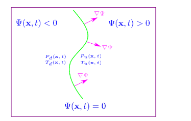
Figure 1.— Illustration of the kinematics of the Biermann effect at a shock surface.

To describe the shock surface, we introduce a level function $\Psi(\mathbf{x},t)$, and use it to define the shock surface $\Psi(\mathbf{x},t)=0$. Note that the function $\Psi$ is of no dynamical significance, but is rather simply a mathematical convenience for describing the shock surface. We will assume that the shock is moving in the direction of the normal vector $\mathbf{n}\equiv\nabla\Psi/|\nabla\Psi|$, so that the region $\Psi(\mathbf{x},t)>0$ is upstream, whereas the region $\Psi(\mathbf{x},t)<0$ is downstream. These definitions are illustrated in Figure 1.

We denote the local shock speed along $\mathbf{n}$ by $D$. By considering the motion of the level surface $\Psi(\mathbf{x},t)=0$ it is not difficult to show that

$$D=-\frac{\partial\Psi}{\partial t}/\left|\nabla\Psi\right|.$$ (13)

To describe a moving MHD discontinuity that coincides with the surface $\Psi(\mathbf{x},t)=0$, we will frequently express a field quantity $X$ by the decomposition $X=X_{u}(\mathbf{x},t)\Theta(\Psi)+X_{d}(\mathbf{x},t)\Theta(-\Psi)$, where $X_{u}$ and $X_{d}$ are continuous functions, and where $\Theta(\Psi)$ is a Heaviside step function. After substituting such expressions into field equations, we will find some terms proportional to the Dirac distribution $\delta(\Psi)$, resulting from differentiation of the Heaviside functions. We will refer to the collected terms of this form as the “shock part” of the evolution equations. As will be seen, such terms embody Rankine-Hugoniot jumps, which can thus be efficiently extracted for these non-symmetric shocks. This trick is also useful for deducing hydrodynamic flux terms, as will also be evident below.

It is convenient to reformulate the Biermann source term using the ideal equation of state to replace $n_{e}$ with $T_{e}$, the electron temperature. Assuming an ideal gas equation of state, the reformulated electric field is

$$\mathbf{E}_{B}\equiv-(k_{B}/e)T_{e}\nabla\ln P_{e},$$ (14)

so that the source term due to the Biermann effect in the induction equation is

$$\left.\frac{\partial\mathbf{B}}{\partial t}\right|_{B}=(ck_{B}/e)\nabla T_{e}\boldsymbol{\times}\nabla\ln P_{e}.$$ (15)

An important reason for this reformulation is that as we saw in §2, in the presence of electron thermal conduction, $T_{e}$ is continuous at the shock, whereas $n_{e}$ is not (Shafranov, 1957; Zel’dovich, Y.B. and Raizer, Y.P., 2002)). As we saw, the continuity of $T_{e}$ is a consequence of the high mobility of electrons relative to ions, and is therefore part and parcel of the same approximation that led to the Biermann source term (Eq. 2) in the first place. It is central to the developments that follow.

The log electron pressure $\ln P_{e}$ is discontinuous at the shock, and may be represented at time $t$ by

$$\ln P_{e}=\ln P_{e,u}\,\Theta\left(\Psi\right)+\ln P_{e,d}\,\Theta\left(-\Psi\right),$$ (16)

where $P_{e,u}(\mathbf{x},t)$ and $P_{e,d}(\mathbf{x},t)$ are continuous functions.

The discontinuity of $P_{e}$ leads to a Dirac-$\delta$ singularity in $\nabla P_{e}$. Using the distributional relation $d\Theta(\Psi)/d\Psi=\delta(\Psi)$, we have

$$\nabla\ln P_{e} = \ln\left(\frac{P_{e,u}}{P_{e,d}}\right)\delta\left(\Psi\right)\nabla\Psi$$

$$+\Theta\left(\Psi\right)\nabla\ln P_{e,u}+\Theta\left(-\Psi\right)\nabla\ln P_{e,d}.$$

We may easily interpret the term in Eq. (LABEL:eq:gradPe) that is proportional to $\delta(\Psi)$ as the gradient proper to the shock, and the remaining terms as the gradient in smooth flow. Since we are interested in the shock behavior, we define

$$\left.\nabla\ln P_{e}\right|_{Shock} \equiv \ln\left(\frac{P_{e,u}}{P_{e,d}}\right)\delta\left(\Psi\right)\nabla\Psi$$ (18)

$$= \ln\left(\frac{\rho_{u}}{\rho_{d}}\right)\delta\left(\Psi\right)\nabla\Psi,$$

where we’ve used the continuity of $T_{e}$ and the assumption of complete ionization to replace the pressure ratio across the shock with the corresponding compression ratio $\rho_{u}/\rho_{d}$.

The electron temperature $T_{e}$ is continuous across the shock, but its normal derivative is discontinuous. We may therefore represent $T_{e}$ by

$$T_{e}=T_{e,u}\Theta\left(\Psi\right)+T_{e,d}\Theta\left(-\Psi\right),$$ (19)

where $T_{e,u}(\mathbf{x},t)$ and $T_{e,d}(\mathbf{x},t)$ are continuous functions, and where continuity at the shock implies

$$\Psi(\mathbf{x},t)=0\Rightarrow T_{e,u}(\mathbf{x},t)=T_{e,d}(\mathbf{x},t).$$ (20)

In virtue of the continuity of $T_{e}$, the gradient $\nabla T_{e}$ is not burdened by a Dirac-$\delta$, and we obtain

$$\nabla T_{e}=\Theta\left(\Psi\right)\nabla T_{e,u}+\Theta\left(-\Psi\right)\nabla T_{e,d}.$$ (21)

Inserting Eqs. (18) and (21) into Eq. (15), we obtain

$$\left.\frac{\partial\mathbf{B}}{\partial t}\right|_{B,Shock} = (ck_{B}/e)\ln\left(\frac{P_{e,u}}{P_{e,d}}\right)\,\delta\left(\Psi(\mathbf{x})\right)$$ (22)

$$\times\left[\frac{1}{2}\left[\nabla T_{e,u}+\nabla T_{e,d}\right]\boldsymbol{\times}\nabla\Psi\right],$$

where we’ve made use of the distributional relation

$$\Theta(\Psi)\delta(\Psi) = \Theta(\Psi)\frac{d}{d\Psi}\Theta(\Psi)$$ (23)

$$= \frac{1}{2}\frac{d}{d\Psi}\Theta(\Psi)^{2}$$

$$= \frac{1}{2}\frac{d}{d\Psi}\Theta(\Psi)$$

$$= \frac{1}{2}\delta(\Psi),$$

where to get the third line, we’ve used the fact that the Heaviside function squares to itself, since its values are either 0 or 1. This derivation of $\Theta\delta=\delta/2$ is admittedly cavalier in its treatment of distributional quantities, and is presented for brevity. The result may also be obtained by a limiting procedure, in which the Heaviside function is represented by the limit of a family of continuous functions – this is, after all, the “Eulerian” limit of the description of a shock as the viscosity goes to zero.

Introducing the shock normal vector $\mathbf{n}$, and using the fact that the tangential derivative of $T_{e}$ is continuous (so that $\mathbf{n}\boldsymbol{\times}\nabla T_{e,u}=\mathbf{n}\boldsymbol{\times}\nabla T_{e,d}$ at the shock), we obtain

$$\left.\frac{\partial\mathbf{B}}{\partial t}\right|_{B,Shock} = \delta\left(\Psi\right)\left|\nabla\Psi\right|\times$$ (24)

$$(ck_{B}/e)\ln\left(\frac{P_{e,u}}{P_{e,d}}\right)\nabla T_{e}\boldsymbol{\times}\mathbf{n}.$$

Eq. (24) is amenable to a clarifying interpretation, which follows from the recognition that if $V$ is a region containing some portion $\Sigma$ of the shock surface, and the differential element of surface area on $\Sigma$ is $dA$, then $\int_{V}d^{3}\mathbf{x}\,\delta(\Psi(\mathbf{x}))|\nabla\Psi|=\int_{\Sigma}dA$, which is to say that $\delta(\Psi(\mathbf{x}))|\nabla\Psi|d^{3}\mathbf{x}$ is the differential area element on the shock surface. We may therefore interpret the quantity $(ck_{B}/e)\ln\left(\frac{P_{e,u}}{P_{e,d}}\right)\nabla T_{e}\boldsymbol{\times}\mathbf{n}$ in Eq. (24) as a field generation rate per unit time per unit area of the shock surface. This interpretation already allows us to see that the Biermann source term should give rise to finite, mathematically sensible field generation.

To verify this, we may now obtain the field generation rate due to the passage of the shock by inserting the above expressions into the induction equation, Eq. (3), neglecting resistivity. The equation may be written as

$$\frac{\partial\mathbf{B}}{\partial t}=\nabla\cdot\left(\mathbf{B}\mathbf{u}-\mathbf{u}\mathbf{B}\right)+\left.\frac{\partial\mathbf{B}}{\partial t}\right|_{B}.$$ (25)

In the neighborhood of the shock, we define

$$\mathbf{B} = B_{n}\mathbf{n}+\mathbf{B}_{Tu}\Theta(\Psi)+\mathbf{B}_{Td}\Theta(-\Psi)$$ (26)

$$\mathbf{u} = \mathbf{u}_{u}\Theta(\Psi)+\mathbf{u}_{d}\Theta(-\Psi)$$ (27)

$$\mathbf{u}_{u} \equiv \mathbf{u}_{Tu}+u_{nu}\mathbf{n}$$ (28)

$$\mathbf{u}_{d} \equiv \mathbf{u}_{Td}+u_{nd}\mathbf{n},$$ (29)

where the “tangential” components satisfy $\mathbf{B}_{Tu}\cdot\mathbf{n}=0$, $\mathbf{B}_{Td}\cdot\mathbf{n}=0$, $\mathbf{u}_{Tu}\cdot\mathbf{n}=0$, $\mathbf{u}_{Td}\cdot\mathbf{n}=0$. In virtue of the solenoidal condition $\nabla\cdot\mathbf{B}=0$, $B_{n}$ is continuous across the shock.

We transform the advection term $\nabla\cdot\left(\mathbf{B}\mathbf{u}-\mathbf{u}\mathbf{B}\right)$ in Eq. (25) by inserting Eqs. (26-27), grouping the Heaviside functions, and collecting the “shock” terms proportional to the Dirac-$\delta$ that arises from differentiating the Heaviside functions. Using Eq. (13) to replace $\partial\Psi/\partial t$, and using Eq. (24), we obtain

$$\delta(\Psi)|\nabla\Psi|(-D)(\mathbf{B}_{Tu}-\mathbf{B}_{Td}) = \delta(\Psi)|\nabla\Psi|\times$$

$$\Big{\{}B_{n}[\mathbf{u}_{Tu}-\mathbf{u}_{Td}]$$

$$-[u_{nu}\mathbf{B}_{Tu}-u_{nd}\mathbf{B}_{Td}]$$

$$+\frac{ck_{B}}{e}\ln\left(\frac{P_{e,u}}{P_{e,d}}\right)\nabla T_{e}\boldsymbol{\times}\mathbf{n}\Big{\}},$$

whence the Rankine-Hugoniot jump condition, generalized by the Biermann flux is

$$\left[(D-u_{n})\mathbf{B}_{T}\right]^{u}_{d}+B_{n}\left[\mathbf{u}_{T}\right]^{u}_{d}+\frac{ck_{B}}{e}\nabla T_{e}\boldsymbol{\times}\mathbf{n}\left[\ln P_{e}\right]^{u}_{d}=0.$$ (32)

Here, the notation $[\ldots]^{u}_{d}$ means the difference of the upstream and downstream values at the shock location. The first two terms in Eq. (32) comprise the usual jump condition for the induction equation (see Chapter 7 of Gurnett & Bhattacharjee, 2005, for example). The final term is the contribution to the jump condition from the Biermann effect, which is seen to produce a finite, well-defined discontinuity at the shock. We may obtain a useful result by considering the jump in $\mathbf{B}$ due to a shock advancing into a quiescent, unmagnetized fluid ($B_{n}=0$, $B_{Tu}=0$, $\mathbf{u}_{u}=0$). The downstream magnetic field is then given by

$$\mathbf{B}_{Td} = \frac{ck_{B}}{e}(D-u_{nd})^{-1}\ln\left(\frac{P_{e,u}}{P_{e,d}}\right)\nabla T_{e}\boldsymbol{\times}\mathbf{n}$$ (33)

$$= \frac{ck_{B}}{eD}\frac{\rho_{d}}{\rho_{u}}\ln\left(\frac{\rho_{u}}{\rho_{d}}\right)\nabla T_{e}\boldsymbol{\times}\mathbf{n},$$

where we’ve used the condition of mass continuity at the shock, $\rho_{u}D=\rho_{d}(D-u_{nd})$, to replace the term $(D-u_{nd})$, and where we’ve also used the continuity of $T_{e}$ to replace the pressure ratio in the log with the density ratio.

We conclude from the above development that the Biermann source term is mathematically well-defined even at weak solution discontinuities, and yields definite finite predictions to which a properly designed numerical algorithm should be expected to converge.

3.2. Physical Compatibility of the Biermann Source Term With Plasma Shock Theory

In the Introduction, we raised the question of whether the Biermann source term, Eq. (2) behaves near a shock according to the predictions of kinetic theory, as summarized in §2. We now explain the line of thinking behind this question, and answer it definitively.

The induction equation, Eq.  (3) can be cast in conservative form. In this form, the Biermann source term assumes the form of the divergence of a flux tensor, whose components are linear in $\nabla P_{e}$. It is clear that the construction of these flux components from the gradient of a discontinuous function is in some way associated with the numerical troubles that arise with the Biermann effect near shocks.

The key point here is that “trouble with a flux computed from a derivative” is actually a familiar situation from radiation diffusion, where the radiation flux, which is proportional to the gradient of the radiation temperature, yields unphysical (superluminal) fluxes at regions where the temperature changes sharply. (see pp. 478-481 of Mihalas & Weibel-Mihalas, 1999, for example). Another analogous situation arises with respect to electron thermal conduction, where the thermal flux from $\nabla T_{e}$ may yield unphysically-large transport at shocks, in consequence of the discontinuous change in $T_{e}$ (Mihalas & Weibel-Mihalas, 1999, p. 302). In both of these cases, a straightforward work-around is furnished by a flux limiter, in which a maximum flux deduced from a kinetic-theory picture of the transport is used to smoothly cut off the flux in regions where gradients get large, while leaving the fluxes in smooth regions unaltered.

This is the reason that the question of the validity of the Biermann flux at shocks is a natural one to ask. If it were the case that the flux is just wrong when $|\nabla P_{e}|$ gets too large, a reasonable approach would be to use the limiting value for the flux from kinetic theory (Eq. 7), and impose that flux in the shock as a cutoff through some kind of flux limiter. If the electric field due to charge separation given by Eq. (2) results in an EMF across a shock that exceeds this value, we could cut it off at this value, and obtain approximate results analogous to flux-limited approximation-based results from diffusion-limited radiation transport.

Being thus prepared for bad news about the Biermann term from kinetic theory, we instead are met by a surprise upon examination of the MHD flux. The Biermann electric field at a shock is, according to Eqs. (14) and (18)

$$\mathbf{E}_{B}=(k_{B}/e)T_{e}\ln\left(\frac{\rho_{d}(\mathbf{x})}{\rho_{u}(\mathbf{x})}\right)\delta\left(\Psi(\mathbf{x})\right)\nabla\Psi.$$ (34)

Integrating this over a vanishingly short shock-crossing path $l$ along the normal to the shock, we obtain the electromagnetic work done by an electron in the presence of the Biermann electric field,

$${\cal E}_{B} = e\int_{l}d\mathbf{x}\cdot\mathbf{E}_{B}$$ (35)

$$= k_{B}T_{e}\ln\left(\frac{\rho_{d}}{\rho_{u}}\right),$$

which is the same as the value inferred from kinetic theory, Eq.(7).

We conclude from this argument that there is no analogy to flux-limited diffusion in the behavior of the Biermann source term at shocks. The “plain vanilla” source gives the correct EMF across the shock, and needs no flux limiter to cut it off there. It should be perfectly possible to construct a physically valid algorithm to represent the Biermann MHD source term unmoderated by limiters, one that faithfully reproduces the predictions of kinetic theory at a shock.

3.3. Origin of the Numerical Biermann Catastrophe

As discussed in the Introduction, MHD simulations incorporating the Biermann Battery effect have invariably produced catastrophic non-convergent behavior as soon as discontinuities develop. There are two (related) kinds of catastrophes that have manifested themselves: simulations with spherical or planar symmetry, in which the charge-separation electric field is irrotational and the magnetic field generation rate should therefore be zero, develop a non-zero field at shocks with a field intensity that grows with increasing resolution (Fatenejad et al., 2013); and simulations of High-Energy-Density Physics (HEDP) laser experiments containing spatially-inhomogeneous shocks, similar to the (highly simplified) simulations presented below in §6.2.2, in which the field generated at shocks, which is not expected to be zero, fails to converge to a finite value with increasing resolution – in order to obtain reasonable results at all in such simulations, the cells participating in shocks, contact, and material discontinuities must be located at each time step, and the generation rate in those cells artificially set to zero (Fatenejad et al., 2013). Such simulation results are clearly not correct, since they do not treat magnetogeneration due to the ion viscous shock, but at least they do converge with resolution.

Clearly something goes very wrong with the numerics when the flow develops discontinuous behavior, whereas the behavior of the Biermann term in smooth flow is finite, convergent, and stable. To investigate the origin of these catastrophes, we have addressed the following question: suppose the electric field $\mathbf{E}_{B}$ of Eq. (15) is irrotational, in the sense that

$$\nabla\boldsymbol{\times}\mathbf{E}_{B}=\frac{k_{B}}{e}\nabla T_{e}\boldsymbol{\times}\nabla\ln P_{e}=0.$$ (36)

To what extent is this irrotational character preserved after $T_{e}$ and $P_{e}$ are separately discretized in a volume-based scheme?

We consider the discretization of two scalar functions $f(\mathbf{x})$ and $g(\mathbf{x})$ that are assumed to have gradients that are everywhere collinear, so that there exists some function $\alpha(\mathbf{x})$ such that $\nabla g=\alpha\nabla f$. A pair of such functions satisfy $\nabla g\boldsymbol{\times}\nabla f=0$, so that the vector field $g\nabla f$ is irrotational. The Taylor series of such a pair of functions are related to each other by the collinearity constraint. We Taylor-expand both functions to third order, average the resulting expansion over a grid of control volumes, and compute the “discrete curl” – that is, the circulation integral about a cell face – of the discretized “$g\nabla f$” vector field. We omit the details of this extremely lengthy calculation for the sake of brevity, and merely present the conclusions that may be drawn therefrom.

The result of the calculation is that the leading-order behavior of the discrete curl of such a discretized vector field is ${\cal O}(\Delta^{2})$, where $\Delta$ is the grid spacing. The coefficient multiplying this term is homogeneous of order 3 in the derivatives of $f$ and $g$. What this means is that in regions of space where the two functions are smooth ($C^{2}$ or smoother), the coefficient has a finite approximation in the discretization, and the discrete curl tends to zero as $\Delta^{2}$ with increasingly fine resolution, yielding the correct curl of an irrotational vector field in the limit.

On the other hand, in the presence of a discontinuity, the coefficient of the discrete curl has no finite approximation in the discretization, but rather diverges as $\Delta^{-3}$ when $\Delta\rightarrow 0$, reflecting the meaninglessness of the Taylor approximation in proximity to a discontinuity. As a consequence, the discrete curl as a whole diverges as $\Delta^{-1}$ with vanishing $\Delta$ in the neighborhood of a discontinuity.

Setting $f=\ln P_{e}$, and $g=T_{e}$, we recognize immediately the source of the discrete pathology described above. The discretization of $P_{e}$ and $T_{e}$ produces a spurious solenoidal component of $\mathbf{E}_{B}$ above and beyond any real, physically-correct solenoidal component. This solenoidal anomaly is small and converges to zero with increasing resolution in smooth flow. Near a discontinuity, however, the anomaly is not convergent, but rather diverges as $\Delta^{-1}$.

This is the explanation of the numerical Biermann catastrophe. It is, fundamentally, a completely predictable failure of naive, stencil-based approximations to the Biermann source term (Eq. 2), which are not meaningful when Taylor-series approximations to the fluid variables fail in the presence of a discontinuity. The failure is irreducible, and doesn’t depend on whether the Biermann flux is added to other MHD fluxes or computed separately as a split term.

3.4. The Cure for the Biermann Catastrophe

The above diagnosis of the origin of the numerical Biermann catastrophe does not directly suggest a cure for the problem. That a cure should exist, however, is strongly suggested by the fact that the analytic treatment of the Biermann effect at shocks in §3.1 leads to finite and physically-sensible field generation rates. We therefore now partly retrace that development with a view to casting those results in a form suitable for formulation as a numerical algorithm to be incorporated in a Godunov-type volume-based MHD scheme.

In order to clarify this proposed strategy, let us briefly review how volume-based hydrodynamics/MHD schemes work (for details, see LeVeque, 2002, for example). Nonlinear systems of hyperbolic PDEs such as MHD are prone to develop discontinuities such as shocks and contacts. Direct finite-difference discretization approaches break down when this occurs. This breakdown is circumvented by appealing to the conservative nature of the equations, and replacing the differential equations with their corresponding conservation-integral forms, applied to a regular mesh of control volumes. Field quantities are interpreted as volume averages over control volumes, and are updated by time-centered (i.e. half-time-step forward) fluxes across control-volume faces. These fluxes are finite even when solution discontinuities cause the corresponding differential PDE source terms to misbehave.

The crucial procedure for carrying out such schemes successfully is the computation of the time-centered fluxes by means of the solution of Riemann shock tube problems at the cell interfaces. A Riemann solver takes as its input piecewise-constant initial data with a discontinuity at the interface and calculates the resulting propagating state, comprising piecewise-constant regions separated by discontinuity waves and rarefactions belonging to different families of characteristics. This propagating state is used to infer the MHD variables at the interface a half-timestep following the initial state. MHD fluxes computed from these variables are then used to update the cell-averaged field quantities (LeVeque, 2002; Toro, 2009).

Riemann solvers relate adjoining MHD states separated by a discontinuity traveling with wave speed $D$ by means of the Rankine-Hugoniot relations,

$$D\times(\bm{\Phi}_{L}-\bm{\Phi}_{R})=\bm{F}(\bm{\Phi}_{L})-\bm{F}(\bm{\Phi}_{R}).$$ (37)

Here, $\bm{\Phi}$ is the state vector of conserved field quantities, $\bm{\Phi}^{T}\equiv[\rho,\rho\mathbf{u}^{T},\rho{\cal E},\mathbf{B}^{T}]$, that is, the mass, momentum, and energy densities and the magnetic field. $\bm{F}$ denotes the vector of fluxes corresponding to $\bm{\Phi}$. The subscripts “L” and “R” denote “Left” and “Right” states, respectively, and $D$ is positive for a wave traveling from Left to Right.(Toro, 2009).

We can now state a minimal requirement in order to assimilate the Biermann flux to the other MHD fluxes used to update the fluid state: We need to establish the terms added by the Biermann effect to the flux vector $\bm{F}$. Once these additive fluxes are determined, they can be added to the ideal MHD fluxes.

The additional flux of $\mathbf{B}$ due to the Biermann effect is obtainable by solving for the shock part of the “Biermann-only” induction equation, Eq. (14). That is to say, we assume the distributional forms of Eqs. (16), (19), and (26), plug them into Eq. (15), and keep only the terms proportional to the dirac-$\delta$. The result may be obtained by inspection of Eq. (32), setting the velocities $\mathbf{u}$ to zero:

$$D(\mathbf{B}_{Tu}-\mathbf{B}_{Td})=-\frac{ck_{B}}{e}\ln\left(\frac{P_{e,u}}{P_{e,d}}\right)\nabla T_{e}\boldsymbol{\times}\mathbf{n},$$ (38)

Comparing Eqs. (38) and (37), and using the continuity of $\nabla T_{e}\boldsymbol{\times}\mathbf{n}$, we obtain for the Biermann effect flux of $\mathbf{B}$ along $\mathbf{n}$

$$\bm{f}_{\mathbf{B}}(\mathbf{n})\equiv-\frac{ck_{B}}{e}\ln(P_{e})\,\nabla T_{e}\boldsymbol{\times}\mathbf{n}.$$ (39)

This expression is manifestly well-defined at discontinuities. As in Eq. (32), from which Eq. (39) is derived, the only residue of the previously toxic gradient $\nabla P_{e}$ is contained in the benign direction vector $\mathbf{n}$, which is effectively $-\nabla P_{e}/|\nabla P_{e}|$ at the shock. The effect of the cross product $\mathbf{n}\boldsymbol{\times}\nabla T_{e}$ is to eliminate the normal component of $\nabla T_{e}$, while leaving only the tangential components. It is clear from the form of Eq. (39) that only the tangential components of $\mathbf{B}$ are subject to change according to the Rankine-Hugoniot condition, as expected.

It is convenient for the purposes of algorithmic implementation to re-express Eq. (39) in tensor form, as an anti-symmetric tensor $\bm{G}^{(B)}$ whose components $G_{ik}^{(B)}$ express the flux in the coordinate direction $k$ of the magnetic field component $B_{i}$:

$$G_{ik}^{(B)}\equiv-\frac{ck_{B}}{e}\ln(P_{e})\sum_{j=1}^{3}\epsilon_{ijk}\frac{\partial T_{e}}{\partial x_{j}},$$ (40)

where $\epsilon_{ijk}$ is the totally anti-symmetric Levi-Civita tensor. $G_{ik}^{(B)}$ is, of course, the spatial part of the dual Maxwell tensor due to the Biermann effect. It is worth pointing out that this expression for the flux tensor differs from the “naive” flux

$$G_{ik}^{(B,Naive)}\equiv+\frac{ck_{B}}{e}T_{e}\sum_{j=1}^{3}\epsilon_{ijk}\frac{\partial\ln(P_{e})}{\partial x_{j}},$$ (41)

obtainable directly from the Biermann electric field (Eq. 14) by a pure gradient, which has no effect on the induction equation. It follows that Eq. (39) yields a general flux of $\mathbf{B}$ in the direction $\mathbf{n}$ that can be used anywhere in the fluid, not only at discontinuities.

The flux in Eq. (39) is not the only correction that must be applied to $\bm{F}$. There is also a correction to be applied to the energy part of the flux vector, in virtue of the Poynting flux $(c/4\pi)\mathbf{E}_{B}\boldsymbol{\times}\mathbf{B}$ that arises in connection with the charge-separation electric field $\mathbf{E}_{B}$. This term is a bit puzzling at first: since $\mathbf{E}_{B}$ is normal to the discontinuity, the Poynting flux is tangential to the discontinuity, and it is not immediately obvious how such a flux is to be pressed into service in a Rankine-Hugoniot relation.

Nonetheless, the required flux may be inferred in a manner analogous to the calculation by which we derived $\bm{F}_{\mathbf{B}}$, above: We solve the “Biermann only” energy equation

$$\frac{\partial(\rho{\cal E})}{\partial t}+\nabla\cdot\left(\frac{c}{4\pi}\mathbf{E}_{B}\boldsymbol{\times}\mathbf{B}\right)=0,$$ (42)

inserting the distributional forms of Eqs. (16), (19), (26), as well as

$$(\rho{\cal E})(\mathbf{x},t)=(\rho{\cal E})_{u}\Theta\left(\Psi\right)+(\rho{\cal E})_{d}\Theta\left(-\Psi\right).$$ (43)

After collecting terms proportional to the Dirac $\delta$, we obtain

$$D\left[\rho{\cal E}\right]^{u}_{d} = \frac{ck_{B}}{4\pi e}\big{[}\left((T_{e}\nabla\ln P_{e})\boldsymbol{\times}\mathbf{n}\right)\cdot\mathbf{B}$$ (44)

$$-\left(\nabla(T_{e}\ln P_{e})\boldsymbol{\times}\mathbf{n}\right)\cdot<\mathbf{B}>$$

$$+T_{e}\ln P_{e}\mathbf{n}\cdot\nabla\boldsymbol{\times}<\mathbf{B}>\big{]}^{u}_{d},$$

where in Eq. (44) we distinguish between $\mathbf{B}$ — the magnetic field to the left or right of the interface — and $<\mathbf{B}>\equiv\frac{1}{2}(\mathbf{B}_{u}+\mathbf{B}_{d})$, the average of the upstream and downstream fields at the interface. Comparing Eq. (44) and Eq. (37), we obtain for the energy flux along $\mathbf{n}$ due to the Biermann effect

$$f_{\rho{\cal E}}(\mathbf{n}) \equiv \frac{ck_{B}}{4\pi e}\big{[}\left((T_{e}\nabla\ln P_{e})\boldsymbol{\times}\mathbf{n}\right)\cdot\mathbf{B}$$ (45)

$$-\left(\nabla(T_{e}\ln P_{e})\boldsymbol{\times}\mathbf{n}\right)\cdot<\mathbf{B}>$$

$$+T_{e}\ln P_{e}\,\mathbf{n}\cdot\nabla\boldsymbol{\times}<\mathbf{B}>\big{]}.$$

Here we see a potential problem: the third term in Eq. (45) requires an average of the upstream and downstream currents $\nabla\boldsymbol{\times}\mathbf{B}$. This is a difficulty if a true flux is to be extracted and pressed into service in a numerical scheme, since possible discontinuities in $\mathbf{B}$ makes such a term ambiguous. The resolution of the difficulty is that in general, there is always some finite resistivity in real plasmas. As we will see below in §4.1, the presence of finite resistivity removes the discontinuity in $\mathbf{B}$, allowing us to replace $<\mathbf{B}>$ with $\mathbf{B}$. We then obtain for the flux of energy in the direction $\mathbf{n}$

$$f_{\rho{\cal E}}(\mathbf{n})=\frac{ck_{B}}{4\pi e}\ln P_{e}\left[\nabla\boldsymbol{\times}\left(T_{e}\mathbf{B}\right)\right]\cdot\mathbf{n}.$$ (46)

To summarize, at a cell interface with a normal vector $\mathbf{n}$, the hydrodynamic fluxes are to be adapted to the Biermann effect by adding to the implemented flux vector $\bm{F}$ an additional flux vector $\bm{F}^{(B)}(\mathbf{n})$, given by

$$\bm{F}^{(B)}=\left(\begin{array}[]{c}\rule[-5.69054pt]{0.0pt}{17.07164pt}F_{\rho}^{(B)}\\ \rule[-5.69054pt]{0.0pt}{17.07164pt}\bm{F}_{\rho\bm{u}}^{(B)}\\ \rule[-5.69054pt]{0.0pt}{17.07164pt}F_{\rho{\cal E}}^{(B)}\\ \rule[-5.69054pt]{0.0pt}{17.07164pt}\bm{F}_{\mathbf{B}}^{(B)}\end{array}\right)\equiv\left(\begin{array}[]{c}\rule[-5.69054pt]{0.0pt}{17.07164pt}0\\ \rule[-5.69054pt]{0.0pt}{17.07164pt}\bm{0}\\ \rule[-5.69054pt]{0.0pt}{17.07164pt}f_{\rho{\cal E}}(\mathbf{n})\\ \rule[-5.69054pt]{0.0pt}{17.07164pt}\bm{f}_{\mathbf{B}}(\mathbf{n})\end{array}\right).$$ (47)

We expect a discretization of the Biermann effect based on these flux expressions to be convergent so long as the mesh resolves the scales on which $T_{e}$ and $\mathbf{B}$ are continuous. The scale at which $T_{e}$ is continuous is the scale length $\lambda_{T}$ of the electron thermal conduction precursor region (Shafranov, 1957; Jaffrin & Probstein, 1964; Zel’dovich, Y.B. and Raizer, Y.P., 2002), discussed in §2.2. This length scale is characteristic of the variation of temperature perpendicular to the shock; however, it is also the length scale over which heat diffuses transversely during the time required for the shock to travel a distance $\lambda_{T}$ (and hence traverse its own thermal precursor). It is therefore the scale to be resolved in order for the discretization of Eq. (39) to converge. At coarser resolutions, $T_{e}$ appears as discontinuous at shocks as all the other fluid variables, and the discretization discussed here will not yield converged results for $\mathbf{B}$. Only as the thermal precursor zone is resolved can convergence be expected.

In order for the discretization to produce convergent results for energy, it is necessary that the simulation resolve the resistive length scale discussed in §4.1. Note, however, that for many physical situations of interest, the magnetic field intensities generated by the Biermann effect are so tiny that the correction due to the Biermann effect to the energy flux may justifiably be neglected – it is dwarfed by the fluxes of thermal and kinetic energy, and possibly also by the advected flux of existing magnetic field energy. Under such circumstances, it is an acceptable approximation to neglect the Biermann energy flux, if a non-resistive calculation is of interest, or if the resistive scale cannot be resolved.

4. Two Novel Physical Effects Arising From Shock Biermann

We now exhibit two novel predictions of the theory of the Biermann effect at shocks. They are the existence of two magnetic precursors to the shock wave, which lead the wave in regions whose extent depends on the upstream conditions: a resistive magnetic precursor, which arises due to magnetogeneration in the shock “leaking” into the upstream fluid in consequence of the presence of finite non-zero resistivity; and a thermal magnetic precursor, due to smooth-flow Biermann-effect magnetogeneration in the fluid motions set up by the electron thermal precursor. We discuss these in turn.

4.1. The Resistive Magnetic Precursor

When the resistivity $\eta$ in the induction equation, Eq. (3) is finite, a new effect appears in the vicinity of a discontinuity: a resistive magnetic precursor travels ahead of the discontinuity, as the impulsively-generated field due to the Biermann effect at the shock diffuses out. This effect is analogous to the well-known electron thermal precursor that precedes a plasma shock, which was discussed in §2.2. The structure of the thermal precursor can be estimated by balancing diffusion and advection of thermal energy in the frame of the shock, in the presence of impulsive shock heating (Zel’dovich, Y.B. and Raizer, Y.P., 2002, pp. 519-520). Similarly, as we will presently see, the structure of the magnetic precursor is a consequence of the balance between magnetic field advection and diffusion in the frame of the shock, in the presence of impulsive magnetogeneration at the shock.

We consider a small portion of the shock surface, which we will treat as approximately planar, and we will work in the rest frame of the shock. We assume an approximately steady state in the shock frame, so that we may set $\partial/\partial t=0$ in the field equations. The induction equation then becomes

$$\nabla\cdot\left(\mathbf{B}\mathbf{u}^{\prime}-\mathbf{u}^{\prime}\mathbf{B}\right)+\nabla\cdot\left(\frac{c^{2}\eta}{4\pi}\nabla\mathbf{B}\right)+\frac{ck_{B}}{e}\nabla T_{e}\boldsymbol{\times}\nabla\ln P_{e}=\bm{0},$$ (48)

where $\mathbf{u}^{\prime}$ is the fluid velocity in the rest frame of the shock.

We will keep only the shock part of the Biermann flux in Eq. (48), that is, the right-hand side of Eq. (24). In effect, this amounts to assuming that the magnetic field generation from the Biermann effect is impulsive at the shock, so that the smooth-flow Biermann effect is much smaller than the effect at the shock. This approximation is justified if the size $\lambda_{T}$ of the electron thermal precursor is much smaller than the size of $\lambda_{B}$ of the magnetic precursor, so that thermal gradients are unimportant except at the discontinuity. The plausibility of this condition will be verified in §4.3.

We may adopt the local simplification $\Psi(\mathbf{x},t)=\mathbf{n}\cdot\mathbf{x}$, $|\nabla\Psi|=|\mathbf{n}|=1$ for the discontinuity-tracing level function. We further adopt coordinates such that $x_{1}$ is along $\mathbf{n}$, so that $\mathbf{n}=\bm{e}_{1}$, and such that $x_{2}$ is along $\nabla T_{e}\boldsymbol{\times}\mathbf{n}$. Away from the discontinuity, we ignore all derivatives except for $\partial/\partial x_{1}$.

The presence of the resistive term changes the discontinuous structure of the solution. This term is the divergence of the resistive flux of $\mathbf{B}$. That flux behaves analogously to the Fick’s law heat flux $-\kappa\nabla T$, in that it opposes gradients in $\mathbf{B}$. A discontinuous $\mathbf{B}$ is disallowed, because it would result in an infinite restoring resistive flux. $\mathbf{B}$ is therefore now continuous. By the Rankine-Hugoniot condition for transverse momentum (Gurnett & Bhattacharjee, 2005, Chapter 7), it follows that $\mathbf{u}_{T}^{\prime}$ is also continuous. Only $u_{n}^{\prime}$ and $P_{e}$ have solution discontinuities in this case. Assuming the upstream fluid is at rest in the lab frame, we therefore set $\mathbf{u}^{\prime}=u_{n}^{\prime}\bm{e}_{1}$, with

$$u_{n}^{\prime}=(-D)\,\Theta(x_{1})+(u_{nd}-D)\,\Theta(-x_{1}).$$ (49)

By the coordinate choice, assuming the far upstream fluid is unmagnetized, and in virtue of Eq. (48), we may set $\mathbf{B}=B\bm{e}_{2}$. Putting this all together, we obtain the following structure equation for the magnetic precursor:

$$\frac{d}{dx_{1}}\left[\frac{c^{2}\eta}{4\pi}\frac{dB}{dx_{1}}-u_{n}^{\prime}B\right]+\delta(x_{1})\frac{ck_{B}}{e}|\nabla T_{e}\boldsymbol{\times}\mathbf{n}| \left[\ln P_{e}\right]^{u}_{d}$$ (50)

$$=0.$$

The meaning of this equation is that the precursor structure is determined by the balance of magnetic diffusion and magnetic advection, in the presence of impulsive magnetic field generation due to the Biermann effect.

In the upstream ($x_{1}>0$) region, we may neglect gradients in $\eta$ (which depends on $T_{e}$). Eq. (50) becomes

$$\frac{c^{2}\eta}{4\pi}\frac{d^{2}B}{{dx_{1}}^{2}}+D\frac{dB}{dx_{1}}=0,$$ (51)

the solution of which, given $\lim_{x_{1}\rightarrow+\infty}B(x_{1})=0$ is

$$B_{u}(x_{1}) = B_{0}\exp\left(-\frac{4\pi D}{c^{2}\eta}x_{1}\right)$$ (52)

$$= B_{0}\exp\left(-\frac{x_{1}}{\lambda_{B}}\right),\quad x_{1}>0.$$

Here, $B_{0}$ is an integration constant. We see that the precursor has an exponential shape and a characteristic length $\lambda_{B}$ given by

$$\lambda_{B}=\frac{c^{2}\eta}{4\pi D}.$$ (53)

Here, $\eta=\eta(T_{e,+\infty})$ is the value of the resistivity far upstream of the discontinuity.

We may obtain a relation for $B_{0}$ from the jump condition at the discontinuity, by integrating Eq. (50) across a vanishingly-small shock crossing path. The result is

$$\frac{c^{2}\eta(T_{e})}{4\pi}\left[\frac{dB}{dx_{1}}\right]^{u}_{d}-\left[u_{n}\right]^{u}_{d}B_{0}+\frac{ck_{B}}{e}|\nabla T_{e}\boldsymbol{\times}\mathbf{n}|\left[\ln P_{e}\right]^{u}_{d}=0,$$ (54)

where now $\eta(T_{e})$ is evaluated at the shock. This condition together with the upstream solution and boundary condition determine $B_{0}$.

The ideal MHD jump conditions may be recovered in the limit of spatially-constant $\eta$ with $\eta\rightarrow 0$. In that case, the downstream solution satisfying finite-$B$ boundary conditions at $x_{1}\rightarrow-\infty$ is $B_{d}(x_{1})=B_{0}$, and the first term in Eq. (54) is just $-DB_{0}$. Eq. (33) follows immediately.

4.2. The Electron Thermal Precursor

One further consequence of the presence of the thermal precursor in $T_{e}$ described in §2.2 is that in general, there will be some small amount of magnetic field generated by the smooth-flow Biermann effect ahead of the shock, due to plasma motions in the preheated region, whose size is $\lambda_{T}$, given by Eq. (6). In general, the field intensity due to this effect can be expected to be small compared to the field intensity due to the resistive magnetic precursor, since the gradients in the thermal magnetic precursor are small compared to those available near the shock itself. In the constant-conductivity simulations that we discuss in §6.2.4, we will see that the field intensity is in fact quite small.

Nonetheless, this smallness does not necessarily preclude the possibility that the thermal magnetic precursor might be experimentally observable. Thermal conductivity upstream of a plasma shock is in general not constant, but rather depends strongly on electron temperature – $\kappa_{e}\sim T_{e}^{5/2}$ (Spitzer, 1962). The actual structure of the thermal precursor is not the gentle exponential decay that one expects for a constant $\kappa_{e}$, but rather exhibits the steep gradient near its outer terminus shown in Figure 7.20 of Chapter VII of Zel’dovich, Y.B. and Raizer, Y.P. (2002). It is possible that this large gradient may be responsible for an enhancement of the Biermann effect at the terminus of the thermal conduction precursor zone. This interesting possibility is beyond the scope of this paper.

One consequence of the presence of a thermal magnetic precursor is that even in a non-resistive approximation, the notion of an un-magnetized fluid upstream of the shock, on which, for example, Eq. (33) is based, is not strictly correct. It is a valid approximation only when the Biermann generation rate in the thermal precursor is small compared to that of the shock.

4.3. Physical Length Scales

It is useful to establish some of the relevant length scales under conditions of interest. Below, we establish these scales for conditions prevailing in HEDP experiments. In §5, we will establish the scales characteristic of galaxy cluster formation.

Using expression for $\eta$ from Huba (2007) in the expression for the resistive magnetic precursor length $\lambda_{B}$ given in Eq. (53), we have the following expression for $\lambda_{B}$ in a fully-ionized plasma:

$$\lambda_{B} = (4/3)(2\pi)^{-1/2}c^{2}e^{2}m_{e}^{1/2}\,Z\ln\Lambda\,D^{-1}(k_{b}T_{e})^{-3/2}$$

$$= 16.4\,\mbox{cm}\times Z\times\frac{\ln\Lambda}{10}$$

$$\times\left(\frac{D}{10^{6}\,\mbox{cm}\,\mbox{s}^{-1}}\right)^{-1}\times\left(\frac{k_{B}T_{e}}{1\mbox{eV}}\right)^{-3/2},$$

(55)

where $\Lambda$ is the usual Coulomb logarithm. Similarly, the expression for the electron thermal precursor length scale $\lambda_{T}$ is (Zel’dovich, Y.B. and Raizer, Y.P., 2002, Chapter VII, §12)

$$\lambda_{T} = \frac{2}{5}\frac{\kappa_{e}(T_{e,0})}{\rho c_{v,e}D}$$

$$= \frac{4}{15}\frac{\xi\,(k_{B}T_{e})^{5/2}}{e^{4}m_{e}^{1/2}ZA\ln\Lambda n_{i}D}$$

$$= 5.39\times 10^{-3}\,\mbox{cm}\times\xi\times Z^{-1}A^{-1}\times\left(\frac{\ln\Lambda}{10}\right)^{-1}$$

$$\times\left(\frac{D}{10^{6}\,\mbox{cm}\,\mbox{s}^{-1}}\right)^{-1}\left(\frac{k_{B}T_{e}}{1\mbox{eV}}\right)^{5/2}\left(\frac{n_{i}}{10^{16}\,\mbox{cm}^{-3}}\right)^{-1},$$

where $T_{e,0}$ is the electron temperature at the shock, and where $\xi$ is a number in the range 1–2.

The numbers in Eqs. (55) and (LABEL:eq:lambda_T_numbers) have been scaled to conditions that are routinely obtainable in large Laser facilities such as Omega and NIF (see, for example Gregori et al., 2012). In these conditions, it is clear that the assumption $\lambda_{T}\ll\lambda_{B}$, required for the validity of the derivation of $\lambda_{B}$, is easily satisfied.

It is also immediately apparent that the magnetic precursor length scale is a macroscopic scale that can in principle be well-tailored to the physical dimensions of the interaction chambers of such facilities. A carefully-designed experiment, which launches a shock into a relatively cold upstream plasma (note the dependence of $\lambda_{B}$ on $T_{e}$) should in principle be able to detect the resistive precursor due to the Biermann effect.

Note that as the value of $T_{e}$ upstream rises, $\lambda_{B}$ decreases as $T_{e}^{-3/2}$, while $\lambda_{T}$ increases as $T_{e}^{5/2}$. We therefore only need to increase the upstream temperature to about 7 eV for $\lambda_{T}$ to become comparable to $\lambda_{B}$, and at warmer temperatures than this $\lambda_{T}$ becomes dominant. It is therefore plausible that a physical situation could be created in which the thermal magnetic precursor might be observable without interference from the resistive magnetic precursor.

5. The Biermann Effect And Galaxy Cluster Formation

In the present section, we attempt to estimate the strength of the seed magnetic fields that result from a correct treatment of the Biermann effect at shocks in galaxy clusters at the time of magnetogenesis ($z\sim 5-3$), and the physical length scales of the resistive magnetic precursor and the electron thermal precursor in this context.

5.1. Proto-Galaxy Cluster Field Generation

As discussed in the introduction, the Biermann effect has been invoked as the source of seed magnetic fields that can be amplified by the turbulent dynamo mechanism (Kulsrud et al., 1997).

Given the fact that in these studies, the gradients near shocks that were used to calculate the Biermann effect field generation rates are artifacts of the hydrodynamic advance schemes, it is possible – even likely – that the calculated field strengths are incorrect. We now attempt to estimate the typical strength of magnetic fields that are to be expected in early galaxy cluster formation, based on a corrected treatment of the Biermann effect. We do not perform new simulations, but rather attempt to estimate the typical field strength based on published simulation data, in a preliminary effort to determine the reliability of field strengths inferred to date in studies of galaxy cluster formation.

While this is not an easy task without actual simulation data on-hand to analyze, the analysis work described in Miniati et al. (2000), based partly on $\Lambda$CDM simulations described in Cen & Ostriker (1994) provides enough information for us to make a rough estimate of the typical field strength. The simulation in question has the properties $H_{0}=60$ km s^-1Mpc^-1, $\Omega_{M}=0.45$, $\Omega_{\Lambda}=0.55$, $\Omega_{b}=0.043$. We now give a relatively detailed description of our analysis of the information in Miniati et al. (2000), in order to make clear both the basis for the estimated field strength and the considerable uncertainty that attend these estimates.

Our starting point is Eq. (33), which gives the post-shock field strength due to the Biermann effect, assuming an unmagnetized upstream fluid. In order to use this equation to estimate field strengths, we need typical values of the shock speed $D$, the compression ratio $\rho_{d}/\rho_{u}$, and the tangential gradient $|\nabla_{\perp}(k_{B}T_{e})|\equiv|\nabla(k_{B}T_{e})\boldsymbol{\times}\mathbf{n}|$ that arise at primordial epochs.

For the sake of exploiting the information available in Miniati et al. (2000), we will choose $z=3$ as our fiducial primordial epoch. Examining the upper-right panel of Figure 8 in Miniati et al. (2000), we conclude that a not-atypical value of $|\nabla_{\perp}(k_{B}T_{e})|$ is

$$|\nabla_{\perp}(k_{B}T_{e})|\approx\frac{k_{B}\times 10^{6}\mbox{K}}{5\mbox{Mpc}}\approx 10^{-35}\,\mbox{erg cm}^{-1},$$ (57)

Neglecting momentarily the fact that the simulation certainly fails to resolve the thermal precursor length scale $\lambda_{T}$ (Eq. 60 below) the uncertainty in this estimate seems to be a factor of 2 or so.

Miniati et al. (2000) supplies shock speeds at redshift $z=0$ (Figure 5 of Miniati et al. (2000)). These may be approximately shifted to $z=3$ using Figure 10 of Miniati et al. (2000), which shows that the kinetic energy processed by shocks increased by a factor of 15 between $z=3$ and $z=0$. This suggests that temperatures increased by about that much (neglecting shock filling-factor differences between the two redshifts), and that velocities increased by about a factor of 4. We had typical shock temperatures of $\sim 10^{6}$ K at $z=3$ in the data leading to the estimate in Eq. (57). This corresponds to a temperature $\sim 10^{7}$ K at $z=0$. From the top-right panel of Figure 5 of Miniati et al. (2000), this corresponds to a shock speed of about $6\times 10^{7}$ cm s^-1 at $z=0$, and hence $D\sim 10^{7}$ cm s^-1 at $z=3$.

Putting these numbers in Eq. (33), and assuming the strong-shock limit $\rho_{d}/\rho_{u}=4$ appropriate to a $\gamma=5/3$ ideal gas, we obtain

$$B=2.9\times 10^{-22}\,\mbox{G}\times\left(\frac{D}{10^{7}\mbox{cm s}^{-1}}\right)^{-1}\times\left(\frac{|\nabla_{\perp}k_{B}T_{e}|}{10^{-35}\mbox{erg cm}^{-1}}\right).$$ (58)

This value should be regarded as a lower limit, since, as remarked above, the simulation does not resolve $\lambda_{T}$. An upper bound on $B$ can be obtained by replacing, in Eq. (57) the 5 Mpc length scale estimated from Figure 8 of Miniati et al. (2000) with $\lambda_{T}$ from Eq. (60). This gives $B\lesssim 10^{-19}$ G; i.e., a value that is a factor of about $10^{3}$ higher. Obviously, this is a very conservative bound, as it assumes temperature fluctuations of order unity over the diffusive scale $\lambda_{T}$.

It is clear from the very uncertain nature of the factors used to construct this estimate that the field strength given in Eq. (58) is itself subject to considerable uncertainty. A few actual MHD simulations with a correct implementation of the Biermann effect seem required to establish how much field strength is in fact made available by the Biermann effect, for turbulent dynamo effects to amplify. Such simulations would be challenging given the spatial scale $\lambda_{T}$ that needs to be resolved.

5.1.1 Galaxy Cluster Formation Length Scales

We now estimate the physical length scales of the resistive magnetic precursor and the electron thermal precursor for the case of galaxy cluster formation using the physical parameters inferred in §5.1 from Miniati et al. (2000) for galaxy cluster formation at $z\simeq 3$. As in §5.1 we use $T_{e}=10^{6}$ K as our reference temperature and $D=10^{7}$ cm s^-1 as our reference shock speed. The assumed cosmological parameter $\Omega_{b}=0.043$ corresponds to a proton number density $n_{i}\approx 10^{-7}$ cm^-3 at $z=0$, and hence to $n_{i}\approx 6\times 10^{-6}$ at $z=3$, which we take as the density upstream of the shocks. With these parameters, the Coulomb logarithm is $\ln\Lambda\approx 40$. Setting $Z=1$, $A=1$, we then have

$$\lambda_{B} = 8.20\times 10^{-3}\,\mbox{cm}\times\frac{\ln\Lambda}{40}$$ (59)

$$\times\left(\frac{D}{10^{7}\,\mbox{cm}\,\mbox{s}^{-1}}\right)\times\left(\frac{T_{e}}{10^{6}\,\mbox{K}}\right)^{-3/2},$$

and

$$\lambda_{T} = 5.01\,\mbox{kpc}\times\xi\times\frac{\ln\Lambda}{40}\times\left(\frac{D}{10^{7}\,\mbox{cm}\,\mbox{s}^{-1}}\right)$$ (60)

$$\times\left(\frac{T_{e}}{10^{6}\,\mbox{K}}\right)^{5/2}\times\left(\frac{n_{i}}{6\times 10^{-6}\,\mbox{cm}^{-3}}\right)^{-1}.$$

The much more tenuous and considerably hotter primordial plasma reverses the relative sizes of $\lambda_{B}$ and $\lambda_{T}$ compared to the HEDP case considered above: $\lambda_{B}$ is now negligible, while $\lambda_{T}$ is an astrophysically-significant length. It is worth comparing $\lambda_{T}$ to $\lambda_{e}$ and $\lambda_{i}$, the expected Spitzer mean free paths of electrons and ions in the plasma, as a consistency check. This is the product of the mean collision time $\tau$ with the thermal speed $(3k_{B}T/m)^{1/2}$. Using the expression for $\tau_{e}$ from Huba (2007), we have

$$\lambda_{e} = \frac{3m_{e}^{1/2}\left(k_{B}T_{e}\right)^{3/2}}{4\sqrt{2\pi}n_{e}\ln\Lambda e^{4}}\times\left(\frac{3k_{B}T_{e}}{m_{e}}\right)^{1/2}$$ (61)

$$= \frac{3\sqrt{3}}{4\sqrt{2\pi}}\frac{\left(k_{B}T_{e}\right)^{2}}{n_{e}\ln\Lambda e^{4}}$$

$$= 2.50\times 10^{-1}\,\mbox{kpc}\,\left(\frac{T_{e}}{10^{6}\,\mbox{K}}\right)^{2}$$

$$\times\left(\frac{\ln\Lambda}{40}\right)^{-1}\times\left(\frac{n_{e}}{6\times 10^{-6}\,\mbox{cm}^{-3}}\right)^{-1}.$$

The mean free path is independent of particle mass, and for $Z=1$ it is the case that $\lambda_{e}=\lambda_{i}$. This length is the characteristic size of the viscous shock sheath, and is reassuringly shorter than the semi-hydrodynamically scaled $\lambda_{T}$.

It is also worth considering whether the plasma is collisional, as we have implicitly assumed by using Spitzer-type transport coefficients. The magnetic field strength estimated in §5.1 gives rise to electron gyroradii $\lambda_{c}$ of characteristic size

$$\lambda_{c} = \left(\frac{3k_{B}T_{e}}{m_{e}}\right)^{1/2}\left(\frac{eB}{mc}\right)^{-1}$$ (62)

$$= 41.4\,\mbox{kpc}\,\left(\frac{T_{e}}{10^{6}\,\mbox{K}}\right)^{1/2}\times\left(\frac{B}{3\times 10^{-22}\,\mbox{G}}\right)^{-1}.$$

Since $\lambda_{c}\sim 100\lambda_{e}$, the flow is comfortably collisional for the chosen physical parameters. An increase in the estimate of $B$ by two orders of magnitude or more would change this conclusion; however, it should be noted that at least at the outset of the process of cosmic magnetogenesis envisioned here, field strengths were probably small enough that the collisional plasma approach is valid. Primordial field strengths that may have originated in early-universe phase transitions or in inflationary scenarios are poorly constrained by theory and observation, but are believed to have plausible values $B<10^{-22}$ G in all but a few scenarios (see Widrow, 2002; Widrow et al., 2012). It follows that initially, at least, the Spitzer-type transport coefficients that we have employed here are likely to be appropriate. This is in contrast to the apparent suppression of electron conductivity at later times (see, e.g. Markevitch et al., 2003; Russell et al., 2012; Sanders et al., 2013; ZuHone et al., 2013).

6. Numerical Verification

6.1. Implementation Using the FLASH Code

We have implemented the corrected Biermann Effect algorithm, described in §3.4, within the publically-available FLASH hydrodynamic simulation framework (Fryxell et al., 2000; Dubey et al., 2009; Tzeferacos et al., 2014). FLASH is a modular and extensible multiphysics scientific simulation software package that has been widely used for reactive compressible flows typical of astrophysical situations, HEDP applications, cosmology, computational fluid dynamics, and fluid–structure interactions. In particular, FLASH makes available both a 2-temperature single-fluid model and resistive MHD, which makes it an ideal platform for testing the proposed algorithm.

Below we furnish an outline of the workings of the code, including the newly-implemented Biermann effect algorithm. Much more detail about FLASH is available in the FLASH Users Guide. We plan to include an implementation of the new Biermann effect algorithm in a future release of the code.

The 2-temperature MHD model that we use for our numerical tests is expressed in conservation form by the following dynamical system:

$$\frac{\partial\rho}{\partial t}+\nabla\cdot\left(\rho\mathbf{u}\right)=0$$ (63)

$$\frac{\partial\rho\mathbf{u}}{\partial t}+\nabla\cdot\left[\rho\mathbf{u}\mathbf{u}-\frac{1}{4\pi}\mathbf{B}\mathbf{B}+\mathbf{1}\left(P+\frac{\mathbf{B}^{2}}{8\pi}\right)\right]=0$$ (64)

$$\frac{\partial}{\partial t}\left[\rho\left(\frac{1}{2}\mathbf{u}^{2}+\epsilon_{T}\right)+\frac{\mathbf{B}^{2}}{8\pi}\right]+\nabla\cdot\bigg{[}\rho\mathbf{u}\left(\frac{1}{2}\mathbf{u}^{2}+\epsilon_{T}+\frac{P}{\rho}\right)+$$

$$\hskip 48.36958pt\frac{1}{4\pi}\left(-\mathbf{u}\boldsymbol{\times}\mathbf{B}+\frac{c^{2}\eta}{4\pi}\nabla\boldsymbol{\times}\mathbf{B}\right)\boldsymbol{\times}\mathbf{B}$$

$$\hskip 48.36958pt+\frac{ck_{B}}{4\pi e}\ln P_{e}\left[\nabla\boldsymbol{\times}\left(T_{e}\mathbf{B}\right)\right]\bigg{]}=0$$ (65)

$$\frac{\partial\rho s_{e}}{\partial t}+\nabla\left(\rho\mathbf{u}s_{e}\right)=-{T_{e}}^{-1}\nabla\cdot\left(-\kappa_{e}\nabla T_{e}\right)$$

$$\hskip 85.35826pt+\frac{\rho c_{v,e}}{T_{e}\tau_{ei}}(T_{i}-T_{e})$$ (66)

$$\frac{\partial\mathbf{B}}{\partial t}+\nabla\cdot\bigg{[}\mathbf{u}\mathbf{B}-\mathbf{B}\mathbf{u}-\frac{c^{2}\eta}{4\pi}\nabla\mathbf{B}+\bm{G}^{(B)}\bigg{]}=0.$$ (67)

These equations differ from Eqs. (8)-(12) only in that the Biermann term in Eq. (65) replaces the one in Eq. (10) to reflect Eq. (46), while the Biermann term in Eq. (67) replaces the one in Eq. (12) to reflect Eq. (40).

FLASH advances the MHD equations using an Unsplit Staggered Mesh (USM) scheme that prevents the development of magnetic monopoles due to numerical noise in the induction equation, and which is described in (Lee, 2013).

The thermal conduction and heat-exchange source terms on the right of Eq. (66) are computed in a time-split manner, separately from the ideal MHD advance. In particular, thermal conduction advance is fully implicit, and works as described in §17.1.4 of the FLASH Users Guide, while heat-exchange operates as described in §16.5 of the FLASH Users Guide. The remaining, advective part of Eq. (66) is implemented by treating $s_{e}$ as a passively-advected mass scalar. This equation requires an EOS implementation capable of using electron entropy as an input variable. For the current case of perfect-gas EOS and total ionization, the standard Sackur-Tetrode equation for entropy is implemented in the EOS.

The resistive terms in Eqs. (65) and (67) are not treated implicitly, but rather are added directly to the MHD fluxes, and are thus treated explicitly, placing diffusive stability limitations on the maximum timestep. The Biermann terms in Eqs. (65) and (67) are also added explicitly to the MHD fluxes. These flux modifications are performed in such a way as to preserve the solenoidal character of the magnetic field, by adding them to the ideal MHD Godunov fluxes before these are interpolated to the edge-centered electric fields of the USM scheme, after which each face-centered normal magnetic field component is updated by the circulation integral of the electric field along the edges bounding the face (Lee, 2013).

We have not performed an analysis of the timestep limitation imposed by the Biermann effect, trusting instead that the small magnitude of the effect in the cases considered makes it unlikely that Biermann timestep constraints could dominate those due to the hyperbolic and diffusive terms. In this connection, it is noteworthy that the Biermann term, being quadratic in fluid derivative terms, makes no contribution to wave dispersion relations obtained by linearization about uniform solutions, and therefore does not appear to affect ordinary wave speeds. Intuitively, one would therefore expect any timestep limitations due to the Biermann effect to be higher-order corrections, hardly affecting the numerical evolution of plasmas for which the Biermann term is small in magnitude. Nonetheless, a full analysis of the effect of the Biermann term on the hyperbolic structure of the system of PDEs would be useful – possibly even necessary – for cases of intense field generation. Such an analysis would be somewhat complicated by the non-quasilinear structure of the Biermann term, necessitating an extension of the PDE system to quasilinear normal form.

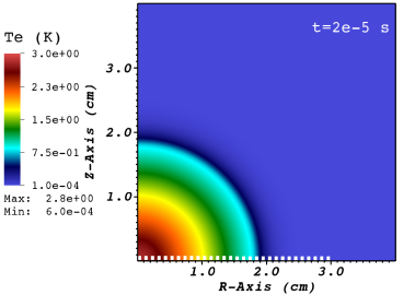
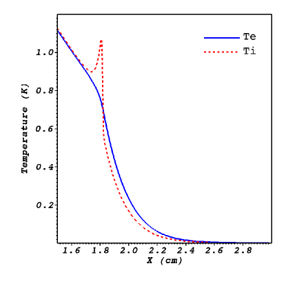
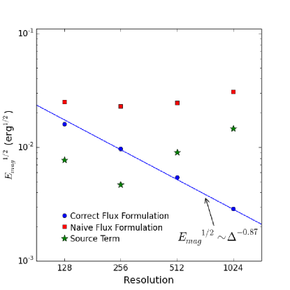
Figure 2.— Two-dimensional simulation of a spherical shock in a 2-temperature Hydrogen plasma. The images refer to the final timestep, at $t=2\times 10^{-5}$ s, and to the highest resolution simulation. Top left: Electron temperature distribution. Top right: Electron and ion temperatures along the shock-crossing line shown at the bottom of the figure in the top left panel. Bottom left: $B_{\phi}$ due to numerical noise. Bottom right: Total magnetic energy as a function of simulation resolution.

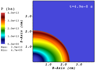
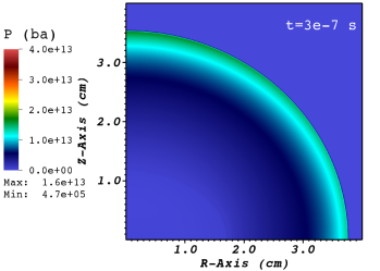
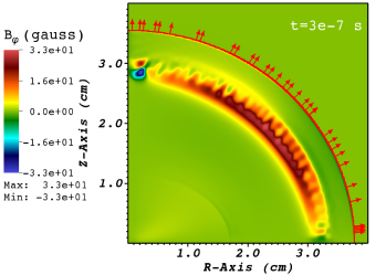
Figure 3.— Ellipsoidal shock. Top Left: Initial pressure distribution; Top Right: Final pressure distribution; Bottom Left: Final magnetic field distribution. The solid red line displays the location of the shock, while the red arrows display the direction of the shock normal; Bottom Right: Difference between final magnetic field distributions computed using the correct and incorrect Biermann flux.

6.2. The Simulations

The simulations presented below represent idealized situations simplified for the sake of verifying the code, and for illustrating the numerical and physical principles under discussion. In particular, the conductivity $\kappa_{e}$, electron-ion equilibration timescale $\tau_{ei}$, and the resistivity $\eta$ are all treated as constants. FLASH does have the capability to use Spitzer-type functions of the thermal state for these parameters, but this would complicate the results unnecessarily without adding any real value to these verification tests.

In what follows, we assume fully-ionized Hydrogen – $A=1$, $Z=1$, adiabatic index $\gamma=5/3$, $c_{v,e}=\frac{3}{2}k_{B}N_{A}$, where $N_{A}$ is Avogadro’s number and $k_{B}$ is Boltzmann’s constant. Simulations are conducted in cylindrical coordinates, assuming azimuthal symmetry, and are therefore 2-dimensional. In addition, we impose a reflection boundary on the $R$-axis (where $R$ is perpendicular distance from axis of rotational symmetry, which is to say, $R$ is the cylindrical radius) so that the domain represents a hemisphere of a solution with reflection symmetry about that axis. In every case, the domain is 4 cm radius cylinder that extends 4 cm in the $z$ direction from the $R$ axis. The boundary conditions at $R=4$ cm and at $z=4$ cm are outflow.

All of the verification tests that we present are variations on the theme of a Sedov-esque explosion: an analytic self-similar Sedov solution is (1) modified to prevent temperatures from diverging at the center by setting all variables constant inside some chosen radius; (2) smoothed with a Gaussian near the shock, to ease instabilities that can otherwise appear near the shock; (3) where required, distorted to an ellipsoidal profile capable of producing real Biermann effect fields; and (4) scaled to velocities and pressures estimated to produce usable simulation times given the resolutions and domain size in play. Values of shock ellipticity, $\kappa_{e}$ and $\eta$ are then chosen to produce reasonable thermal and magnetic precursor region sizes, and reasonable field generation rates, and values of $\tau_{ei}$ are chosen to be harmless. In every case, we run an initial model for a time without the Biermann effect, so as to allow transients in the 2-temperature hydrodynamic variables to subside. Then we restart the calculation with Biermann field generation turned on.

Magnetic fields are always azimuthal in these verification tests – since the gradients of $T_{e}$ and $P_{e}$ are always in the $R-z$ plane the Biermann effect only generates non-zero field along the azimuthal direction.

6.2.1 Null Test: A Spherical Shock

It is not a simple matter to construct a non-trivial analytic verification solution of a plasma generating magnetic field through the Biermann effect. A trivial solution, on the other hand, may be straightforwardly constructed by imposing symmetry requirements that align the gradients $\nabla P_{e}$ and $\nabla T_{e}$, thus guaranteeing zero field generation. We use a spherical Sedov-like explosion as an example of such a test. This is in fact the test that revealed the Biermann catastrophe in the first place (Fatenejad et al., 2013).

We assume an initial shock radius of 1.15 cm, in an ambient medium with $\rho=1$ g cm^-3 and $P$ set to a negligible value. We choose an initial velocity scale inside the shock that leads to a shock velocity that is on average about $3.2\times 10^{4}$ cm s^-1 during the course of the simulation. Other physical parameters are $\kappa_{e}=1.0\times 10^{12}$ erg K ^-1 cm^-1 s^-1 and $\tau_{ei}=2\times 10^{-14}$ s. The initial solution is advanced for $10^{-5}$ s with no field generation, then re-started and run for another $10^{-5}$ s with field generation turned on. We repeated this experiment with the correct Biermann flux term of Eq. (40), with the naive flux of Eq. (41), and with the time-split source term of Eq. (15), so as to compare the performance of the three algorithms.

The results of this study are displayed in Figure 2. The top-left panel is a colormap view of the electron temperature $T_{e}$. The dashed shock-crossing line across the bottom of this figure is the location of the data displayed in the top-right panel, which shows electron and ion temperatures. The shock is visible as the peak in $T_{i}$. The thermal precursor is clearly visible, as is the continuous behavior of $T_{e}$, which changes slope at the shock in accordance with standard plasma shock theory (Zel’dovich, Y.B. and Raizer, Y.P. 2002, Chapter VII, §12). The ion temperature also rises in the precursor region in consequence of the electron-ion equilibration term.

The lower-left panel of Figure 2 shows the magnetic field strength generated by the correct treatment of Eq. (40). There is spurious non-zero field due to numerical noise that is clearly being generated. However, the lower-right panel shows that this field is converging to zero with increasing resolution. This figure displays the square-root of the total magnetic energy in the domain. Since the analytic solution for the magnetic field strength is zero everywhere, this quantity functions as an un-normalized $L^{2}$-norm of the difference between the analytic and numerical solutions. The blue circles show the convergence with resolution of the correct formulation. This convergence behavior is in contrast to the behavior of the other two algorithms, which fail altogether to converge.

6.2.2 Verification With An Ellipsoidal Shock

Next we exhibit simulations designed to produce non-zero values of the magnetic field strength. We start an ellipsoidal shock surface, obtained by distorting the spherical Sedov solution. The initial configuration has a semi-major axis (aligned with the $R$-axis) of 2 cm, and a semi-minor axis (aligned with the $z$-axis) of 1.667 cm. The ambient medium is uniform with $\rho=1$ g cm^-3 and $P$ set to a negligible value. We choose a velocity scale that leads to shock velocities of the about $6\times 10^{6}$  cm s^-1. The higher shock speed is chosen to produce somewhat intense magnetic field strengths. To keep the thermal precursor resolved, we increase the conductivity to $\kappa_{e}=1.0\times 10^{13}$ erg K^-1 cm ^-1 s^-1. We also set $\tau_{ei}=10^{-14}$ s. The initial solution is advanced for $4.86\times 10^{-8}$ s with no field generation, then re-started and advanced to a simulation time $t=3\times 10^{-7}$ s with field generation turned on.

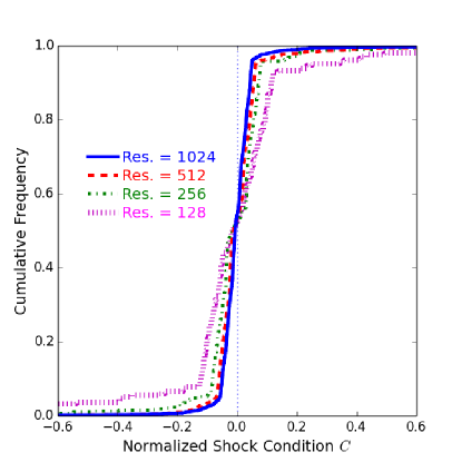
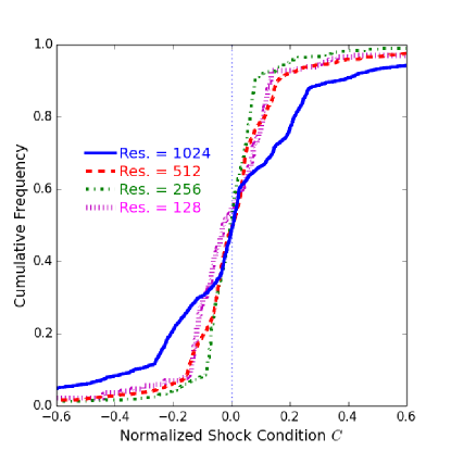
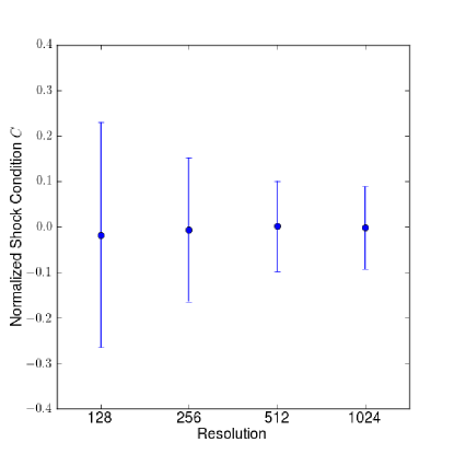
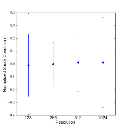
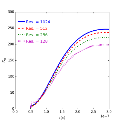
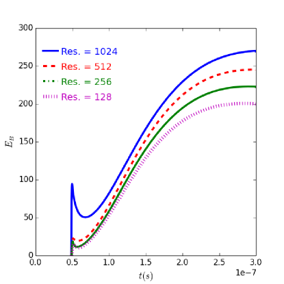
Figure 4.— Left Panels: Correct Biermann flux term. Right Panels: “Naive” Biermann flux term. Top Panels: Cumulative distribution of the normalized magnetic shock condition $C$, defined by Eq. (73), evaluated at points along the shock surface, for four different resolutions, illustrating convergence to the correct jump condition. Middle Panels: sample standard deviations of $C$, as a function of resolution. Bottom Panels: Total magnetic energy as a function of simulation time for the four resolutions studied.

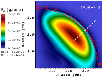
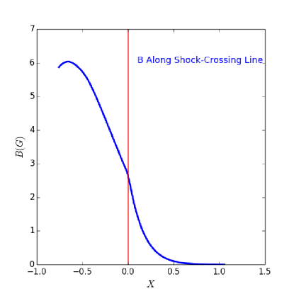
Figure 5.— Left Panel: Magnetic field distribution due to passage of shock, in the presence of finite resistivity. The simulation differs from the one shown in Figure 3 only by the presence of non-zero resistivity. The solid red line shows the location of the shock, while the vectors represent the unit normal to the shock. The magnetic precursor can be clearly seen ahead of the shock surface. The white dashed shock-crossing line illustrates the location of the data displayed in the right panel. Right Panel: Magnetic field strength magnitude along the white dashed shock-crossing line shown in the left panel. The position of the shock is shown by the vertical solid red line. The predicted exponential decay of the precursor is evident.

The advance of the shock during the period when magnetic field is generated is illustrated by the two pressure colormap plots in the top panels of Figure 3. The lower-left panel of Figure 3 shows the magnetic field intensity generated according to the correct flux of Eq. (40), ranging into the tens of Gauss. The solid red line in the figure shows the shock location, while the red arrows display the shock unit normal vector. The lower-right panel displays the difference between the correct and the naive flux formulations, which is substantial at the outgoing shock surface.

We do not have an analytical solution for the magnetic field distribution to compare to the output of these simulations. We do, however, have the relation between shock quantities expressed by Eq. (32), which determines the jump condition for $\mathbf{B}$. By locating points adjoining the shock, and computing the local shock velocity at those points, we can then verify that Eq. (32) in fact obtains, to some accuracy limited by the numerical approximation. This is in principle a non-trivial verification, since the code does not know about the jump condition Eq. (32) as such – it only knows the fluxes expressed by Eq. (40), which were inferred from the jump condition. Recovery of the jump condition thus constitutes a verification that the code correctly models the theory.

To perform this verification, we first locate cells adjoining the shock by the method described in Appendix A, which yields a 1-cell wide shock surface by fitting the mass, momentum, and energy Rankine-Hugoniot conditions to the neighboring data, using a speed-of-sound weighted inner-product on the state space, and treating the shock speed $D$ as a free fit parameter. The shocked cells are the ones that fit the R-H conditions with small fit residuals ($R^{2}<0.01$), together with some other natural auxiliary consistency conditions described in the Appendix. The fitted shock speed is then used in the verification of Eq. (32).

In the absence of normal component field $B_{n}$, Eq. (32) becomes

$$(D-u_{d})B_{d}-(D-u_{u})B_{u}$$

$$+\frac{ck_{B}}{e}\left(n_{z}\frac{\partial T_{e}}{\partial R}-n_{R}\frac{\partial T_{e}}{\partial z}\right)\left[\ln P_{e,d}-\ln P_{e,u}\right]\equiv$$

$$a_{d}-a_{u}+b_{d}-b_{u}=0,$$ (68)

where we’ve defined “Advection” terms $a_{u,d}$ and “Biermann” terms $b_{u,d}$ by

$$a_{d} \equiv (D-u_{d})B_{d}$$ (69)

$$a_{u} \equiv (D-u_{u})B_{u}$$ (70)

$$b_{d} \equiv \frac{ck_{B}}{e}\left(n_{z}\frac{\partial T_{e}}{\partial R}-n_{R}\frac{\partial T_{e}}{\partial z}\right)\ln P_{d}$$ (71)

$$b_{u} \equiv \frac{ck_{B}}{e}\left(n_{z}\frac{\partial T_{e}}{\partial R}-n_{R}\frac{\partial T_{e}}{\partial z}\right)\ln P_{u}.$$ (72)

The sum of terms in Eq. (68) is required to be zero. In a discretized numerical PDE integration, this really means that the terms must cancel up to some truncation or rounding precision, which is expressed relative to the largest of the magnitudes in play. We therefore define the “shock condition parameter” $C$ by

$$C\equiv\frac{a_{d}-a_{u}+b_{d}-b_{u}}{\mbox{max}(|a_{d}|,|a_{u}|,|b_{d}|,|b_{u}|)}.$$ (73)

We calculate the value of $C$ at cells along the shock front, at each of our four resolution levels, for both the correct flux and the “naive” flux implementations of the Biermann effect. We display cumulative distributions of $C$ in the top panels of Figure 4. It is evident from these figures that the distribution of $C$ is in fact centered near zero for both flux implementations. The width of the distributions behave very differently, however. In the case of the correct Biermann flux implementation, the distributions get narrower with each refinement of resolution, providing some evidence of convergence with resolution to the expected result. In the case of the naive flux implementation, there is no such evidence of convergence. The same observations can be made of the plots in the middle panels of Figure 4, which summarize the means and sample standard deviations of the $C$-distributions, as a function of resolution. The convergence of the correct flux implementation, and the convergence failure of the naive implementation, are clear in these figures.

The bottom panels of Figure 4 show the evolution of total magnetic energy in the domain as a function of time, for the different resolutions and for the two flux implementations. The correct flux implementation appears to be converging (although not in any strong sense converged) by this measure, even at late time, whereas any evidence of convergence in magnetic field energy is simply lacking for the naive flux implementation.

6.2.3 The Resistive Magnetic Precursor

In this set of simulations, we maintain the simulation parameters described in §6.2.2, but also turn on the resistivity $\eta$ to a finite positive value, $\eta=7.8\times 10^{5}$ s ^-1, chosen in conjunction with the other parameters to yield an easily-discernible exponentially-decaying resistive precursor described by Eq. (52). We repeat the simulation strategy of §6.2.2, letting the simulation advance to $t=4.86\times 10^{-8}$ s with no field generation, then re-starting it and advancing to a simulation time $t=3\times 10^{-7}$ s with field generation (using the correct flux formulation) turned on. This advance time is adequate for the establishment of the expected precursor structure, as we demonstrate below.

The left panel of Figure 5 shows a colormap of the distribution of magnetic field strength across the domain. The shock location is shown by the solid red line, and the superposed vectors indicate the shock-normal direction. The magnetic field is evidently smoothed out by the resistivity, as can be seen by a direct comparison with the bottom-left panel of Figure 3. The precursor is already evident in this figure, as the substantial amount of magnetic field that has “leaked” ahead of the shock.

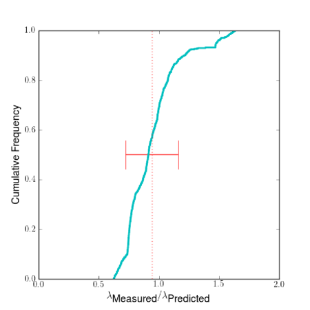
Figure 6.— Cumulative distribution of the measured magnetic precursor decay length, normalized to the predicted length, at 849 points along the shock surface. The mean is shown by the dotted line, while the standard deviation is illustrated by the errorbar.

The diagonal white dashed shock-crossing in the left panel of Figure  5 illustrates the line along which data was extracted to produce the right panel of Figure 5. This figure shows the magnetic field values plotted along that line. The vertical solid red line at $X=0$ marks the location of the shock. The exponential decay of the field is easily visible in this figure.

At each shock location, the value of $\eta$ can be combined with the local shock velocity to calculate $\lambda_{\mbox{Predicted}}$, the expected decay length of the precursor, according to Eq. (53). At the same time, the actual decay length $\lambda_{\mbox{Measured}}$ can be measured directly by comparing the field strength at two suitably-selected distances along the local shock normal. We have performed both calculations at each shock location, and compared them. The results are displayed in Figure 6, where we plot the cumulative distribution of $\lambda_{\mbox{Measured}}/\lambda_{\mbox{Predicted}}$. The distribution appears to be consistent with a mean value of 1, as expected, with some scatter. The scatter is not surprising, since the expression in Eq. (53) for $\lambda_{\mbox{Predicted}}$ is an approximation, assuming, as it does, propagation of magnetic field from a planar shock. Since the shock is, of course, not planar, the value of the Biermann generation rate changes appreciably across the shock over distances not hugely different from $\lambda_{\mbox{Predicted}}$ itself. Under the circumstances, then, the level of agreement between observation and prediction is satisfactory.

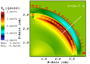
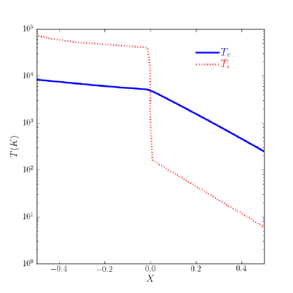
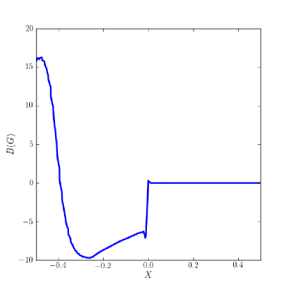
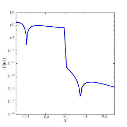
Figure 7.— Ellipsoidal shock, with 10$\times$ greater thermal conductivity. Top Left: Final magnetic field distribution. The solid red line shows the shock location, while the arrows show the direction of the shock normal. The white dashed shock-crossing line illustrates the location of the data displayed in the remaining panels; Top Right: Electron and ion temperatures along the white dashed shock-crossing line in the previous panel. The shock location and thermal precursor are evident; Bottom Left: $B$ along the shock-crossing line; Bottom Right: Semilog plot of $|B|$ along shock-crossing line.

6.2.4 The Thermal Magnetic Precursor

In our final simulation, we explore the properties of the thermal magnetic precursor by returning to a non-resistive simulation, similar to the ones discussed in §6.2.2, and differing from them only in that $\kappa_{e}$ is ten times larger: $\kappa_{e}=1.0\times 10^{14}$ erg K^-1 cm ^-1 s^-1. This broadens the thermal precursor zone to about 0.2 cm, making it easier to discern.

The results at the final time step are illustrated in Figure 7. The top-left panel shows the distribution of magnetic field in the domain. The solid red line in the figure shows the location of the shock, while the arrows show the direction of the shock normal. In the top-right panel we see the electron and ion temperatures along the shock-crossing line shown in the previous panel. The shock location coincides with the sharp drop in $T_{i}$, while the thermal conduction precursor zone, which has an exponential structure for the constant conductivity model used here, may be clearly seen in the upstream behavior of $T_{e}$.

The magnetic field structure along the shock-crossing line is shown in the bottom-left panel of the figure. The precursor is difficult to see in this plot, so the bottom-right panel shows $|B|$ on a semi-log plot. The magnetic precursor structure is seen in this figure. It clearly has a much lower field intensity than the fields generated by the Biermann effect at the shock. We emphasize again, however, that in part this is due to the highly simplified constant-conductivity model adopted for this work. A true Spitzer-type conductivity, with a $T_{e}^{5/2}$ dependence, would create much sharper gradients at the upstream termination of the precursor zone, potentially generating more intense fields – relative to those generated at the shock – than those shown here.

7. Summary and Discussion

To summarize our findings: Using the kinetic theory of plasma shocks, we have given a description of the Biermann effect within ion viscous shocks. Using this description, we have shown that the convergence failures in the presence of shocks of MHD codes implementing the Biermann effect is not traceable either to a mathematical mis-specification of the Biermann term – which is well-defined despite appearances – or to a failure of the Biermann MHD source term to correctly approximate the expected physics. The failure is instead due to naive discretization, a condition that we have shown is curable by exploiting the continuity of the electron temperature $T_{e}$.

We have described a convergent algorithm that incorporates the Biermann effect within shocks in numerical MHD, and implemented it in the FLASH code. We have developed and used verification tests to demonstrate formal convergence using a null solution from spherical shock, and to verify predictions for physical conditions near a shock using an ellipsoidal shock. Comparisons of the new algorithm, which provides a correct and accurate treatment of the Biermann effect within shocks, with the previous, naive one exhibit clearly desirable physical and numerical properties present in the new algorithm that were previously wanting.

We have noticed, described, and simulated two previously unrecognized physical effects: a resistive magnetic precursor that leads the shock in the presence of non-zero resistivity, and that is analogous to the well-known thermal precursor caused by the presence of finite electron thermal conduction; and a thermal magnetic precursor, produced by plasma motions in the electron thermal conduction precursor. We have estimated the expected magnitude of both effects in conditions encountered in laboratory experiments at laser facilities, and shown that the characteristic length of the two effects can be made macroscopic. In particular, the resistive magnetic precursor is physically measurable in an experimental setup that measures both the position of the shock front and a time-series of the intensity of the magnetic field at some location initially ahead of the shock. Such an experiment would have to somehow ensure that the upstream fluid remains unheated by shock-generated radiation and by laser absorption, so as to keep the value of the resistivity high enough to sustain a macroscopically-scaled precursor length. The thermal magnetic precursor may be more challenging to observe, as it is intrinsically weaker than the resistive precursor (relative to the field intensity generated at the shock). Further studies with Spitzer-type electron thermal conductivity are needed to determine whether sharp gradients at the upstream termination of the electron thermal precursor can give rise to sufficiently intense magnetic field strengths to be experimentally measurable.

We emphasize again that the requirement for convergence in $\mathbf{B}$ of the new Biermann effect algorithm is that the electron thermal precursor of the shock should be resolved, while the requirement for convergence in magnetic energy of the new algorithm is that the resistive precursor should be resolved. Of these two requirements, the first is more essential, because neglect of the contribution of the Biermann effect to the flux of magnetic energy is frequently a valid approximation. Demanding resolution of the electron thermal precursor is not a trivial requirement in realistic simulations. It certainly mandates some kind of Adaptive Mesh Refinement (AMR) strategy to resolve the region near the shock. But irrespective of AMR-related efficiencies, merely resolving that length scale can constrain the code to taking very short time steps due to the Courant-Friedrichs-Lewy (CFL) stability condition, unless an implicit advancement scheme is implemented for MHD. This issue is the subject of current study, but it lies beyond the scope of the present paper.

With the discussion of the modification due to the Biermann effect of the Rankine-Hugoniot jump condition on $B$ – Eq. (32) and text thereabout – it now seems worth returning to the question of vorticity $\bm{\omega}$, and the beguiling Equation (5) that suggests its proportionality to $\mathbf{B}$. Recall that much hangs on the jump conditions – if the jump in $\bm{\omega}$ maintains the same proportionality to the jump in $\mathbf{B}$ as do their respective evolution equations, then, subject to some cavils about boundary conditions, $\mathbf{B}$ is simply $\bm{\omega}$, at least until resistivity and/or viscosity manifest themselves, and in effect, unmagnetized gasdynamics contains within it the magnetic degrees of freedom of MHD, encoded in derivatives of the velocity field.

It can be seen more clearly now why this implausible assertion is in fact false. In the first place, $\mathbf{B}$ and $\bm{\omega}$ are rather different types of quantities from the point of view of kinetic theory, in that $\mathbf{B}$ is perfectly well-defined at kinetic scales – such as inside an ion viscous shock sheath – whereas $\bm{\omega}$ cannot even be defined consistently in regions where the fluid picture breaks down. The jump condition on $\mathbf{B}$ is a straightforward consequence of the induction equation, and is essentially kinematic in origin, as are the other Rankine-Hugoniot conditions. The jump condition on vorticity, on the other hand, cannot be inferred from the dynamical PDE equations alone, but depends in an essential manner on the equation of state (Kevlahan, 1997). It would be possible, in principle, to infer a “flux” of $\bm{\omega}$ from Eq. (4), and to construct a “jump condition” using that flux in the Rankine-Hugoniot conditions, Eq. (37). That jump condition would disagree with the one obtained in (Kevlahan, 1997), as it is manifestly independent of the EOS. The EOS dependence of the jump condition on vorticity implies that even if there exists an EOS according to which the jump condition on $\bm{\omega}$ preserves the required proportionality to the Biermann-laden jump in $\mathbf{B}$, that proportionality would certainly not be preserved for any other EOS.

In general, then, the passage of a shock certainly spoils Eq. (5). This should be no surprise, as the manipulations of the hydrodynamic equations of motion required to arrive at Eq. (4) constitute precisely the sorts of prestidigitation with vector derivatives that break down at fluid discontinuities (see p. 216 of LeVeque, 2002, for example). While Eq. (4) may be derived from the momentum equation on either side of the shock, the connection between $\mathbf{B}$ and $\bm{\omega}$ is certain to be lost at the shock itself, well before resistive and viscous effects can assert themselves. We conclude that the vorticity connection is not a useful tool for studying magnetogeneration by the Biermann effect in the presence of shocks.

In concluding, it is worth pointing out again that since shocks are not the only weak-solution discontinuities that arise in multi-material MHD simulations, they are not the only locations where potential convergence failures are corrected by the new algorithm. In particular, contact discontinuities, material discontinuities, and ionization fronts all present potential problems for the naive Biermann algorithm, since they all represent locations where $P_{e}$ changes discontinuously (despite the continuity of total pressure $P$ at such locations), and are therefore all sites where the Biermann effect can be expected to generate magnetic field. They all represent physical situations in which the new algorithm provides a correct treatment of the Biermann effect.

Appendix A Shock Detection

We describe here our shock detection algorithm, which we used in the verification of the Biermann effect at shocks. This algorithm has some benefits over shock-detection algorithms such as the ones described in Balsara & Spicer (1999); Miniati et al. (2000); Ryu et al. (2003), in that it furnishes an estimate of the shock speed directly from a single time slice of spatial data, weights the mass, momentum, and energy components of the Rankine-Hugoniot relations equally, yields a single-cell-wide shock interface, verifies that local characteristics converge on the shock surface, and does not impose arbitrary thresholds on physical quantities such as compression ratios or Mach numbers.

We start with a mesh of cells containing fluid values (for present purposes it is immaterial whether these are cell averages or point values). The algorithm seeks a set of “shocked” cells satisfying the following criteria:

• The Shocked Surface Is One Cell Wide: Each shocked cell is the location of a maximum of $|\nabla P|$ in the direction of $\nabla P$, where $P$ is the total fluid pressure;

• Fluid Quantities Change Correctly: The neighborhood of each shocked cell exhibits compression, acceleration, and heating in the direction of $\nabla P$;

• Rankine-Hugoniot Conditions Obtain: The full Rankine-Hugoniot conditions on mass, momentum, and energy hold between the fluid upstream and downstream of each shocked cell, where “upstream” means in the direction $\mathbf{n}\equiv-\nabla P/|\nabla P|$;

• Characteristics Converge On The Shock Surface: The characteristic convergence criterion holds at each shocked cell: the shock is supersonic upstream, and subsonic downstream.

The result is an efficient and reliable algorithm that among other things yields an accurate estimate of the shock speed, which is essential to our verification work on the Biermann effect. Note that we neglect the induction equation in the shock detection algorithm, and operate using only the material pressure – not the total pressure, which includes the magnetic pressure. For weakly magnetized plasmas, such as the ones we consider in this paper, this creates no difficulty in identifying the correct shock surface. Some generalization would be required for significantly magnetized plasmas, particularly to the third and fourth conditions above.

We now describe in somewhat greater detail the algorithm outlined above.

A.1. The Shocked Surface Is One Cell Wide

The first condition above is tantamount to insisting that the shocked cell be sited at a position where the gradient of $P$ is steepest. In general, volume-based hydrodynamic advance schemes spread shocks over several cells. If we were not to impose this condition, we would obtain a thickened shell of shocked cells, which would complicate the criterion (specified below) for classifying neighboring cells as adjoining the shock upstream or downstream.

The condition is very easy to enforce: in the immediate neighborhood of the cell being tested for “shockedness”, we check the adjoining cells closest to the direction of the normal vector $\mathbf{n}$ and its mirror image $-\mathbf{n}$. This is done by forming the vector of integers $\Delta\bm{i}\equiv\mbox{NINT}[\mathbf{n}/\mbox{max}(n_{1},n_{2},n_{3})]$ (where the NINT function ascribes the nearest integer to each component of its real vector argument) and adding it to the cell discrete index vector $\bm{i}$, to reach the cells at $\bm{i}\pm\Delta\bm{i}$. If a stencil-based estimate of $|\nabla P|$ is greater in the candidate cell than in the two so-chosen adjoining cells, then the condition is passed successfully.

A.2. Fluid Quantities Change Correctly

An easy sanity check for “shockedness” of a cell is that cells downstream should unfailingly be (a) compressed, (b) accelerated (in the $+\mathbf{n}$ -direction), and (c) heated, with respect to cells upstream.

We introduce a shock-width parameter $h$, such that the shock-adjoining cells “upstream” and “downstream” of the shocked cell are respectively located at $\pm h\times\Delta\times\mathbf{n}$ relative to the cell under study, where $\Delta$ is the length of a cell side. For FLASH with the HLL Riemann solver (Toro, 2009) and 2nd-order reconstruction, an appropriate value of $h$ is 1.5. We then simply verify that the fluid variables $\rho$, $\mathbf{u}$, and $e_{T}$ (the total thermal energy) satisfy the conditions $\left[\rho\right]^{d}_{u}>0$, $\left[\mathbf{u}\cdot\mathbf{n}\right]^{d}_{u}>0$, and $\left[e_{T}\right]^{d}_{u}>0$.

A.3. Rankine-Hugoniot Conditions Obtain

The Rankine-Hugoniot (R-H) conditions, which express flux conservation in the frame of the shock, have the form

$$D\times(\bm{\Phi}_{d}-\bm{\Phi}_{u})=\bm{F}(\bm{\Phi}_{d})-\bm{F}(\bm{\Phi}_{u}).$$ (A1)

Here, $\bm{\Phi}$ is the state vector of conserved field quantities, $\bm{\Phi}^{T}\equiv[\rho,\rho\mathbf{u}\cdot\mathbf{n},\rho{\cal E}]$, that is, the mass, normal momentum, and energy densities. $\bm{F}$ denotes the vector of fluxes corresponding to $\bm{\Phi}$. The subscripts “d” and “u” denote “downstream” and “upstream” states, respectively (Toro, 2009).

We fit R-H conditions to the upstream/downstream data defined using the shock-width parameter $h$ above. In this fit, the shock speed $D$ is a free parameter to be adjusted to minimize a fit residual. Given a positive-definite inner product $\left[\Phi_{1},\Phi_{2}\right]$ on the vector state space in Eq. (A1), we may define the normalized residual $R^{2}$ as

$$R^{2}\equiv\frac{\left[\left(D\Delta\bm{\Phi}-\Delta\bm{F}\right),\left(D\Delta\bm{\Phi}-\Delta\bm{F}\right)\right]}{\left[\Delta\bm{F},\Delta\bm{F}\right]},$$ (A2)

where $\Delta\bm{\Phi}\equiv\bm{\Phi}_{d}-\bm{\Phi}_{u}$ and $\Delta\bm{F}\equiv\bm{F}(\bm{\Phi}_{d})-\bm{F}(\bm{\Phi}_{u})$. We may then easily minimize $R^{2}$ with respect to $D$, obtaining

$$D_{Min} = \frac{\left[\Delta\bm{\Phi},\Delta\bm{F}\right]}{\left[\Delta\bm{\Phi},\Delta\bm{\Phi}\right]}$$ (A3)

$$R^{2}_{Min} = 1-\frac{\left[\Delta\bm{F},\Delta\bm{\Phi}\right]^{2}}{\left[\Delta\bm{F},\Delta\bm{F}\right]\left[\Delta\bm{\Phi},\Delta\bm{\Phi}\right]}.$$ (A4)

Given these definitions, we consider that the R-H conditions are satisfied if $R^{2}_{Min}$ is less than some small threshold value.

It remains to define the inner product $[\cdot,\cdot]$ used in these expressions. It is obvious that the naive unweighted sum-of-squares of the components of vectors such as $\Delta\bm{\Phi}$ is not an acceptable inner product, as it is dimensionally senseless. We require at a minimum a positive-definite metric that brings all vector components to the same physical dimensions, so we don’t wind up adding mass densities to energy densities, and so on. An additional desirable requirement is that all three components of Eq. (A1) should contribute similar magnitudes to Eqs. (A3) and (A4), so that they are all weighted equally in the fit.

A simple metric that accomplishes these requirements may be build using the local sound speed $c_{s}$ of the candidate shocked cell:

$$\left[\bm{\Phi}_{1},\bm{\Phi}_{2}\right]\equiv{\bm{\Phi}_{1}}^{T}\bm{M}\bm{\Phi}_{2},$$ (A5)

where

$$\bm{M}\equiv\left[\begin{array}[]{lll}1&0&0\\ 0&{c_{s}}^{-2}&0\\ 0&0&{c_{s}}^{-4}\\ \end{array}\right].$$ (A6)

This choice produces compatible dimensions and comparable magnitudes, because in and downstream of the shock we have $c_{s}\sim(k_{B}T/m_{i})^{1/2}\sim D$, so that in the frame of the shock, the mass flux is $\rho D\sim\rho c_{s}$, the momentum flux has magnitude $P\sim\rho{c_{s}}^{2}$, and the energy flux has magnitude $\rho D^{3}\sim\rho{c_{s}}^{3}$.

We adopt this metric in computing Eqs. (A3) and (A4). We find that a threshold of $R^{2}_{Min}<0.01$ is adequate for identifying cells satisfying the R-H conditions with few false-positives and false-negatives, in the simulations exhibited in this paper.

A.4. Characteristics Converge On The Shock Surface

Our final criterion is easily stated and checked: shocks are supersonic upstream, and subsonic downstream, so that characteristics from the family implicated in the shock converge on the shock (see Courant & Friedrichs, 1948, pp. 141-146). This is an essential stability criterion for the solution. Using the shock speed $D_{Min}$ calculated while fitting the R-H conditions to the data, this condition is simply

$$\mathbf{u}_{d}\cdot\mathbf{n}+c_{s,d}>D_{Min}>\mathbf{u}_{u}\cdot\mathbf{n}+c_{s,u},$$ (A7)

where $c_{s,d}$ and $c_{s,u}$ are the downstream and upstream sound speeds, respectively, as determined with respect to the shock width $h$ defined above.

References

- Amendt et al. (2009) Amendt, P., Milovich, J., Wilks, S., Li, C., Petrasso, R., & Séguin, F. 2009, Plasma Physics and Controlled Fusion, 51, 124048
- Balsara & Spicer (1999) Balsara, D. S., & Spicer, D. S. 1999, Journal of Computational Physics, 149, 270
- Biermann (1950) Biermann, L. 1950, Zeitschrift Naturforschung Teil A, 5, 65
- Bryan et al. (2014) Bryan, G. L. et al. 2014, ApJS, 211, 19
- Cen & Ostriker (1994) Cen, R., & Ostriker, J. P. 1994, ApJ, 429, 4
- Courant & Friedrichs (1948) Courant, R., & Friedrichs, K. 1948, Supersonic flow and shock waves, Pure and applied mathematics (Interscience Publishers)
- Davies & Widrow (2000) Davies, G., & Widrow, L. M. 2000, The Astrophysical Journal, 540, 755
- Drake (2006) Drake, R. 2006, High-Energy-Density Physics: Fundamentals, Inertial Fusion, and Experimental Astrophysics, High pressure shock compression of condensed matter (Springer)
- Dubey et al. (2009) Dubey, A., Antypas, K., Ganapathy, M. K., Reid, L. B., Riley, K., Sheeler, D., Siegel, A., & Weide, K. 2009, Parallel Computing, 35, 512
- Fatenejad et al. (2013) Fatenejad, M. et al. 2013, High Energy Density Physics, 9, 172
- Fryxell et al. (2010) Fryxell, B. et al. 2010, High Energy Density Physics, 6, 162
- Fryxell et al. (2000) Fryxell, B. et al. 2000, ApJS, 131, 273
- Gnedin et al. (2000) Gnedin, N. Y., Ferrara, A., & Zweibel, E. G. 2000, The Astrophysical Journal, 539, 505
- Gregori et al. (2012) Gregori, G. et al. 2012, Nature, 481, 480
- Gurnett & Bhattacharjee (2005) Gurnett, D., & Bhattacharjee, A. 2005, Introduction to Plasma Physics: With Space and Laboratory Applications (Cambridge University Press)
- Huba (2007) Huba, J. 2007, 2007 Plasma Formulary - Handbook of Data and Tables for Plasma Physics and Engineering (Wexford College Press)
- Jaffrin & Probstein (1964) Jaffrin, M., & Probstein, R. 1964, Physics of Fluids, 7, 1658
- Kevlahan (1997) Kevlahan, N.-R. 1997, Journal of Fluid Mechanics, 341, 371
- Kronberg (1994) Kronberg, P. P. 1994, Reports on Progress in Physics, 57, 325
- Kulsrud et al. (1997) Kulsrud, R. M., Cen, R., Ostriker, J. P., & Ryu, D. 1997, The Astrophysical Journal, 480, 481
- Kulsrud & Zweibel (2008) Kulsrud, R. M., & Zweibel, E. G. 2008, Reports on Progress in Physics, 71, 046901
- Lee (2013) Lee, D. 2013, Journal of Computational Physics, 243, 269
- LeVeque (2002) LeVeque, R. 2002, Finite Volume Methods for Hyperbolic Problems, Cambridge Texts in Applied Mathematics (Cambridge University Press)
- Markevitch et al. (2003) Markevitch, M. et al. 2003, ApJ, 586, L19
- Meinecke et al. (2014) Meinecke, J. et al. 2014, Nature Physics, 10, 520
- Mihalas & Weibel-Mihalas (1999) Mihalas, D., & Weibel-Mihalas, B. 1999, Foundations of Radiation Hydrodynamics, Dover Books on Physics (Dover)
- Miniati et al. (2000) Miniati, F., Ryu, D., Kang, H., Jones, T. W., Cen, R., & Ostriker, J. P. 2000, ApJ, 542, 608
- Russell et al. (2012) Russell, H. R. et al. 2012, MNRAS, 423, 236
- Ryu et al. (2003) Ryu, D., Kang, H., Hallman, E., & Jones, T. 2003, The Astrophysical Journal, 593, 599
- Sanders et al. (2013) Sanders, J. S., Fabian, A. C., Churazov, E., Schekochihin, A. A., Simionescu, A., Walker, S. A., & Werner, N. 2013, Science, 341, 1365
- Shafranov (1957) Shafranov, V. D. 1957, Soviet Physics JETP, 5, 1183
- Smith et al. (2013) Smith, B., O’Shea, B. W., Voit, G. M., Ventimiglia, D., & Skillman, S. W. 2013, ApJ, 778, 152
- Spitzer (1962) Spitzer, L. 1962, Physics of Fully Ionized Gases … Second Revised Edition, [Interscience Tracts on Physics and Astronomy. no. 3.] (New York, London)
- Srinivasan & Tang (2013) Srinivasan, B., & Tang, X.-Z. 2013, Physics of Plasmas (1994-present), 20, 056307
- Subramanian et al. (1994) Subramanian, K., Narasimha, D., & Chitre, S. M. 1994, MNRAS, 271, L15
- Toro (2009) Toro, E. 2009, Riemann Solvers and Numerical Methods for Fluid Dynamics: A Practical Introduction (Springer)
- Tzeferacos et al. (2014) Tzeferacos, P. et al. 2014, High Energy Density Physics, accepted, DOI http://dx.doi.org/10.1016/j.hedp.2014.11.003
- Tzeferacos et al. (2012) ——. 2012, High Energy Density Physics, 8, 322
- Widrow (2002) Widrow, L. M. 2002, Reviews of Modern Physics, 74, 775, astro-ph/0207240
- Widrow et al. (2012) Widrow, L. M., Ryu, D., Schleicher, D. R. G., Subramanian, K., Tsagas, C. G., & Treumann, R. A. 2012, Space Sci. Rev., 166, 37, 1109.4052
- Xu et al. (2010) Xu, H., Li, H., Collins, D. C., Li, S., & Norman, M. L. 2010, The Astrophysical Journal, 725, 2152
- Xu et al. (2011) ——. 2011, The Astrophysical Journal, 739, 77
- Xu et al. (2008) Xu, H., O’Shea, B. W., Collins, D. C., Norman, M. L., Li, H., & Li, S. 2008, The Astrophysical Journal Letters, 688, L57
- Zel’dovich, Y.B. and Raizer, Y.P. (2002) Zel’dovich, Y.B. and Raizer, Y.P. 2002, Physics of shock waves and high-temperature hydrodynamic phenomena (Dover Pubns)
- ZuHone et al. (2013) ZuHone, J. A., Markevitch, M., Ruszkowski, M., & Lee, D. 2013, ApJ, 762, 69