Infinite densities for Lévy walks

Abstract

Motion of particles in many systems exhibits a mixture between periods of random diffusive like events and ballistic like motion. In many cases, such systems exhibit strong anomalous diffusion, where low order moments $\langle|x(t)|^{q}\rangle$ with $q$ below a critical value $q_{c}$ exhibit diffusive scaling while for $q>q_{c}$ a ballistic scaling emerges. The mixed dynamics constitutes a theoretical challenge since it does not fall into a unique category of motion, e.g., the known diffusion equations and central limit theorems fail to describe both aspects. In this paper we resolve this problem by resorting to the concept of infinite density. Using the widely applicable Lévy walk model, we find a general expression for the corresponding non-normalized density which is fully determined by the particles velocity distribution, the anomalous diffusion exponent $\alpha$ and the diffusion coefficient $K_{\alpha}$. We explain how infinite densities play a central role in the description of dynamics of a large class of physical processes and discuss how they can be evaluated from experimental or numerical data.

I Introduction

The trajectory of a particle embedded in a complex or even some seemingly simple structures may exhibit simultaneous modes of motion r_arkady_pik ; Strong . An example is deterministic transport of a tracer particle in an infinite horizon ordered Lorentz billiard, a set of fixed circular hard scatterers arranged in a square lattice Bou85 ; Zacharel ; Bouchaud ; Artuso ; Armstead ; Sanders ; Courbage . A tracer moving freely among a set of scatterers and bouncing elastically once encountering one of them, exhibits intermittent behavior with long flights where the particle moves ballistically, separated by collision events which induce a diffusive like motion. A similar behavior of the tracing particle can be induced by the flow acting in the phase space of chaotic Hamiltonian systems 2dHam1 ; 2dHam2 . The key to our discussion are power law distributed waiting times between collision events, induced by the geometry of the scatterers Bouchaud ; Levitz ; BarkaiLL ; Wiersma . A condition for such non-Drude like dynamics is that the radii of scatterers is smaller than half the lattice spacing and that the tracer is a point like particle, hence the tracer has an infinite horizon Bouchaud ; Sanders . Also consider the very different type of motion of polymeric particles in living cells, where sub-diffusive motion is separated by long power law distributed flights which induce super-diffusion Naama . Such systems are difficult to characterize since they exhibit at least two modes of motion. A common tool in the analysis of such data is the spectrum of exponents $q\nu(q)$ Strong . One measures the $q$-th moment of the motion, for particles starting on a common origin

$$\langle|x(t)|^{q}\rangle\sim t^{q\nu(q)}$$ (1)

with $q>0$. Here, for sake of simplicity we consider the one dimensional case and avoid other possible time dependencies like a logarithmic increase of moments with time. Scale invariant transport implies that $\nu(q)$ is a constant independent of $q$, for example, for Brownian motion $\nu(q)=1/2$. In many fields of science one finds that $\nu(q)$ is a non-linear function of $q$, the term strong anomalous diffusion is often used in this context Strong . Surprisingly, in many cases the continuous spectrum $q\nu(q)$ exhibits a bi-linear scaling (see details below). Examples for this piecewise linear behavior of $q\nu(q)$ include nonlinear dynamical systems Strong ; Artuso ; Armstead ; Sanders ; Courbage , stochastic models with quenched and annealed disorder, in particular, the Lévy walk Andersen ; GL ; Zabu1 ; r_vezzani ; Burioni ; Bernabo and sand pile models Sandpile . Recent experiments on the active transport of polymers in the cell Naama , theoretical investigation of the momentum KesslerPRL and the spatial DechantPRL spreading of cold atoms in optical lattices and flows in porous media Anna further confirmed the generality of strong anomalous diffusion of the bi-linear type. An example is a diffusive scaling $q\nu(q)=q/2$ below a certain value of $q_{c}>0$ and a ballistic scaling $q\nu(q)=q-q_{c}/2$ otherwise. This is an example of a motion which is neither purely diffusive nor ballistic.

While the mechanisms leading to strong anomalous diffusion could be vast, even the stochastic treatment of such systems is not well understood. For example, diffusion equations, either normal or fractional Review , stochastic frameworks like fractional Brownian motion or generalized Langevin equations Goy and the Gauss-Lévy central limit theorem Bouchaud ; levy fail to describe this phenomena. We recently investigated the Lévy walk process Shles ; KBS ; Klafter ; ZK ; Cristadoro , a well known stochastic model of many natural behaviors which exhibits bi-linear strong anomalous diffusion. Examining four special cases we found that a non-normalizable density, with a diverging area underneath it, describes these processes gang4 . This unusual infinite density, describes the ballistic aspects of strong anomalous diffusion. Here we find a general formula for the infinite density which, as we show below, is complementary to the Gauss and Lévy distributions. The latter are the mathematical basis of many diffusive phenomena, and here we promote the idea that the infinite density concept is a rather general tool statistically characterizing the ballistic trait of the motion. We show how these unnormalized distributions emerge from a basic model with wide applications, thus, possibly this overlooked measure may become an important tool.

In mathematics the concept of a non-normalized infinite density was thoroughly investigated Thaler1 ; Aaronson ; Thaler while in physics this idea has gained interest only recently (see below). Conservation of matter implies that the number of particles in the system is fixed, thus naturally one may normalize the probability density describing a packet of non-interacting diffusing particles $P(x,t)$ to unity $\int_{-\infty}^{\infty}P(x,t){\rm d}x=1$. Hence dynamical and equilibrium properties of most physical systems are described by densities which are normalized, for example, a Boltzmann-Gibbs state in thermal equilibrium, or solutions of Boltzmann or Fokker-Planck equations with normalization conserving boundary conditions (no absorbing boundaries). However, in some cases a closer distinction must be made, namely a distinction based on the observable of interest. Probably the most common averaged observables are the moments $\langle|x|^{q}\rangle$ of a process $x(t)$, so in this example the observable is $|x(t)|^{q}$ and we will distinguish between high order moments $q>q_{c}$ and low order ones. In our case we treat a system with mixed dynamics, and show that the low order moments are described by the standard machinery of non-equilibrium statistical physics (fractional diffusion equations and Lévy central limit theorem) but the high order moments, which represent the ballistic elements of the process, are described by an infinite density. In this sense the infinite density is complementary to the central limit theorem gang4 . We find a general formula for this infinite density relating it to the velocity distribution of the particles, the anomalous diffusion exponent $\alpha$ and the diffusion constant $K_{\alpha}$. Our work shows how the unnormalized state emerges from the norm conserving dynamics of the Lévy walk. Previous work KesslerPRL ; KorabelPesin ; Miya01 ; Akimotoprl ; KorabelINF ; KorabelNum ; LutzNature ; Holz on applications of the infinite density in physics, dealt with bounded systems which attain an equilibrium. For example the momentum distribution of cold atoms where the Gibbs-measure is finite the infinite density describes the large rare fluctuations of the kinetic energy KesslerPRL ; Holz . Or intermittent maps with unstable fixed points, e.g., the Pomeau-Manneville transformation on the unit interval KorabelPesin ; Akimotoprl . Here we consider systems that are not in equilibrium, and the dynamics is unbounded, showing that the potential applications of infinite densities are vast.

II Lévy walk model

In the Lévy walk process the trajectory of the particle $x(t)$ consists of epochs of ballistic travel separated by a set of collisions which alter its velocity Bouchaud ; Review ; Shles ; Klafter ; ZK . At time $t=0$ the particle is on the origin. Its initial velocity $-\infty<v_{0}<\infty$ is random and drawn from a probability density function (PDF) $F(v)$, whose moments are all non-diverging LWbasic . The particle travels with a constant speed for a random duration $\tau_{1}>0$ whose PDF is $\psi(\tau)$. The particle’s displacement in this first sojourn time is $v_{0}\tau_{1}$. At time $t_{1}=\tau_{1}$ we draw a new velocity $v_{1}$ and a waiting time $\tau_{2}$ from the corresponding PDFs $F(v)$ and $\psi(\tau)$. The second displacement is $v_{1}\tau_{2}$. This process is renewed. The waiting times $\{\tau_{i}\}$ ($i=1,2,\cdots$) and the velocities $\{v_{j}\}$ ($j=0,1,\cdots$) are mutually independent identically distributed random variables. The points on the time axis $t_{N}=\sum_{i=1}^{N}\tau_{i}$ are the collision times, when the particle switches its velocity. The position of the particle at time $t$ is

$$x(t)=\sum_{j=1}^{N}v_{j-1}\tau_{j}+v_{N}\tau_{b}\>.$$ (2)

Here $N$ is the random number of collisions or renewals in the time interval $(0,t)$. The time interval $\tau_{b}=t-t_{N}$ is called the backward recurrence time GL . The last term in Eq. (2) describes the motion between the last collision event and the measurement time $t$

$$t=\sum_{j=1}^{N}\tau_{j}+\tau_{b}\>.$$ (3)

A model where $N$ is fixed and $t$ is random, namely, a process stopped after $N$ collisions (so $\tau_{b}=0$) is the classical problem of summation of independent identically distributed random variables for which the Lévy-Gauss central limit theorem applies levy .

As already mentioned, we assume that $F(v)=F(-v)$ hence from symmetry the density of particles $P(x,t)$ is also symmetric since all particles start on the origin. We also assume that the even moments of $F(v)$ are finite, hence the tail of $F(v)$ decays faster than any power law. The PDF of waiting times is given in the long time limit by

$$\psi(\tau)\sim{A\over|\Gamma(-\alpha)|}\tau^{-1-\alpha}\>,$$ (4)

where $A>0$ and

$$1<\alpha<2\>.$$ (5)

As discussed briefly in the summary, our main finding, that a non-normalized infinite density describes the density of particles $P(x,t)$, is found also for $\alpha\geq 2$, but for simplicity of presentation we consider only a limited interval for $\alpha$. The case $1<\alpha<2$ corresponds to enhanced diffusion $\langle x^{2}\rangle\propto t^{3-\alpha}$ which is faster than normal diffusion but slower than ballistic Klafter . The regime $\alpha<1$, is called the ballistic phase of the motion since then $\langle x^{2}\rangle\propto t^{2}$. For that case and for a general class of the velocity PDF, $F(v)$, the PDF $P(x,t)$ is given by a formula in Rebenshtok ; Rebenshtok1 . The case $\alpha>2$ corresponds to normal diffusion in the mean square displacement sense $\langle x^{2}\rangle\propto t$.

A convenient tool is the Laplace transform of the waiting times PDF denoted

$$\hat{\psi}(u)=\int_{0}^{\infty}\exp(-u\tau)\psi(\tau){\rm d}\tau\>.$$ (6)

For a power law distributed waiting time under investigation, i.e., $1<\alpha<2$, and for small $u$ the following expansion holds Review ; ZK ; GL ; Carry

$$\hat{\psi}(u)=1-\langle\tau\rangle u+Au^{\alpha}+\cdots$$ (7)

where $\langle\tau\rangle=\int_{0}^{\infty}\tau\psi(\tau){\rm d}\tau$ is the averaged waiting time.

III Some background on the Lévy walk

The position of the particle is rewritten as

$$x=\sum_{i=1}^{N}\chi_{i}+\chi^{*}$$ (8)

where $\chi_{i}=v_{i-1}\tau_{i}$ are the flight lengths and $\chi^{*}=v_{N}\tau_{b}$. Since the velocity distribution is narrow and symmetric, the PDF of flight lengths $q(\chi)$ is also symmetric $q(\chi)=q(-\chi)$. Since the durations of the flights are power law distributed we have

$$q(\chi)\propto|\chi|^{-(1+\alpha)}$$ (9)

for large $|\chi|$. In the regime $0<\alpha<2$ the variance of jump length is infinite hence the Gaussian central limit theorem does not apply. In the regime $1<\alpha<2$ the average waiting time $\langle\tau\rangle$ is finite. Neglecting fluctuations, the number of flights is $N=t/\langle\tau\rangle$ when $t$ is long. Hence in this over-simplified picture we are dealing with a problem of a sum of $N$ independent identically distributed random variables with a common PDF $q(\chi)$ with a diverging variance. In this picture the last jump $\chi^{*}$ is negligible. Thus, one may argue that $x$ is described by Lévy’s generalized central limit theorem. This means that the PDF of $x$ is expected to be a symmetric Lévy stable law Kotulski (see details below). However, such a treatment ignores the correlations between flight durations and flight lengths and the fluctuations of $N$. In fact the finite speed of the particles implies that jumps much larger than the typical velocity times the measurement time $t$ are impossible. Thus, the mean square displacement and higher order moments always increase slower than ballistic, for example $\langle x^{2}\rangle<\mbox{const}\ t^{2}$. In contrast, a sum of independent identically distributed random variables with an infinite variance, often called a Lévy flight, yields a diverging mean square displacement $\langle x^{2}\rangle=\infty$. For that reason Lévy walks, which take into consideration the finite velocity, are considered more physical if compared with Lévy flights Strong ; Klafter . Since both the Gauss and the Lévy central limit theorems break down in the description of moments of Lévy walks, more specifically in the tails of the PDF of $x$, it is natural to ask if there exists a mathematical replacement for these widely applied theorems.

A more serious treatment of the Lévy walk is given in terms of the Montroll-Weiss equation. Let $P(x,t)$ be the PDF of the position of particles at time $t$ for particles starting at the origin. From the mentioned symmetry of the process $P(x,t)=P(-x,t)$, $P(x,t)|_{t=0}=\delta(x)$ so clearly all odd moments of $P(x,t)$ are zero. We define the Fourier-Laplace transform

$$P(k,u)=\int_{-\infty}^{\infty}{\rm d}x\int_{0}^{\infty}{\rm d}t\exp(ikx-ut)P(x,t)\>.$$ (10)

The Montroll-Weiss equation gives the relation between the distributions of the model parameters namely velocities and waiting times with $P(k,u)$ KBS ; ZK ; Carry

$$P(k,u)=\left\langle{1-\hat{\psi}(u-ikv)\over u-ikv}\right\rangle{1\over 1-\left\langle\hat{\psi}\left(u-ikv\right)\right\rangle}\>.$$ (11)

Here the averages are with respect to the velocity distribution $\langle...\rangle=\int_{-\infty}^{\infty}{\rm d}v\cdots F(v)$. The derivation of this classical result is provided in an Appendix. Note that in the original work of Montroll and Weiss a decoupled random walk was considered and the origin of Eq. (11) can be traced to the work of Scher and Lax Lax and that of Shlesinger, West and Klafter Shles (see also KBS ; ZK ; Carry ; pathways ; Kutner ; Marcin ). Examples Klafter ; Bouchaud ; Review for physical processes described by the Lévy walk are certain non-linear dynamical systems Artuso ; Shles ; Strong ; Solomon , polymer dynamics Ott , blinking quantum dots Jung ; Margprl ; Marg ; Hoog , cold atoms diffusing in optical lattices Sagi ; KesBarPRL , intermittent search strategies Benichou , dynamics of perturbations in many body Hamiltonian systems Zabu ; Figueiredo ; Spohn , and particle dynamics in plasmas Zimbardo .

In what follows we naively expect that one can reconstruct the normalized density of particles in the long time limit from the exact expressions for the moments of the process. Specifically, we obtain the exact expression for the long time limit of the integer moments of the Lévy walk process $\langle x^{2n}(t)\rangle$ with $n=1,2,..$, where the case $n=0$ is trivial since $\langle x^{0}\rangle=\int_{-\infty}^{\infty}P(x,t){\rm d}x=1$, and then we use the moments to consruct a series equivalent to the Fourier transform of the density

$$\langle\exp(ikx)\rangle=\int_{-\infty}^{\infty}e^{ikx}P(x,t){\rm d}x=1+\sum_{n=1}^{\infty}{\langle(ikx)^{2n}\rangle\over(2n)!}.$$ (12)

Luckily, we can evaluate analytically the sum for the model under consideration. Then we perform the inverse Fourier transform of the such obtained function. One then naively expects to get the long time limit of the density $P(x,t)$ since we use the long time limit of the moments. It turns out that this procedure yields a density which is not normalizable (for reasons which will become clear later). However, while the solution is not normalizable, it still describes the density of particles $P(x,t)$ in ways which will hopefully become more transparent to the reader by the end of the manuscript.

IV The Moments

To obtain the long time behavior of spatial moments $\langle x^{2n}(t)\rangle$ we first find the Laplace transforms $\langle x^{2n}(u)\rangle$. Here, as mentioned, odd moments are zero due to the assumed symmetry $F(v)=F(-v)$. For that aim we use the well known expansion

$$P(k,u)=\int_{-\infty}^{\infty}e^{ikx}P(x,u){\rm d}x=\int_{-\infty}^{\infty}\left[1+\sum_{n=1}^{\infty}{(ikx)^{2n}\over(2n)!}\right]P(x,u){\rm d}x={1\over u}+\sum_{n=1}^{\infty}{(ik)^{2n}\langle x^{2n}(u)\rangle\over(2n)!}\>.$$ (13)

Expanding the numerator and denominator of the Montroll-Weiss equation, Eq. (11) using the expansion Eq. (7), to the leading order in the small parameter $u^{\alpha-1}$, while keeping the ratio $k/u$ fixed, we get

$$P(k,u)\sim{1-\tilde{A}u^{\alpha-1}\langle\left(1-{ikv\over u}\right)^{\alpha-1}\rangle\over u\left[1-\tilde{A}u^{\alpha-1}\langle\left(1-{ikv\over u}\right)^{\alpha}\rangle\right]}\>$$ (14)

with $\tilde{A}=A/\langle\tau\rangle$. As is well known, such small $u$ expansions correspond to the long time limit Review ; GL . Further expanding the denominator to find the first non-trivial term we obtain

$$P(k,u)\sim{1\over u}\left\{1-\tilde{A}u^{\alpha-1}\left[\left\langle\left(1-{ikv\over u}\right)^{\alpha-1}\right\rangle-\left\langle\left(1-{ikv\over u}\right)^{\alpha}\right\rangle\right]+\cdots\right\}\>.$$ (15)

The leading $(1/u)$ term is obviously the normalization condition $P(k,u)|_{k=0}=1/u$. In this expansion we included terms of the order $u^{\alpha-1}$, while higher order terms, which are found from further expansion of the denominator in Eq. (14), but also non-universal terms which stem from the expansion of $\hat{\psi}(u)$, Eq. (7), to orders greater than $u^{\alpha}$, are neglected. We Taylor expand Eq. (15) in $k/u$, using the series expansion

$$\left(1-\epsilon\right)^{\alpha-1}-\left(1-\epsilon\right)^{\alpha}=-\sum_{m=1}^{\infty}{(-\alpha)_{m}\epsilon^{m}\over\alpha(m-1)!}\>,$$ (16)

where $(a)_{m}=\Gamma(a+m)/\Gamma(a)=a(a+1)\cdots(a+m-1)$ is the Pochhammer symbol. Averaging over velocities we find

$$P(k,u)\sim{1\over u}-\tilde{A}\sum_{n=1}^{\infty}{(2n)(-\alpha)_{2n}(-1)^{n}\over(2n)!(-\alpha)}u^{\alpha-2-2n}\langle v^{2n}\rangle k^{2n}\>$$ (17)

with $\langle v^{2n}\rangle=\int_{-\infty}^{\infty}v^{2n}F(v){\rm d}v$. Comparing with Eq. (13) yields in the small $u$ limit

$$\langle x^{2n}(u)\rangle\sim{\tilde{A}\over\alpha}(-\alpha)_{2n}(2n)\langle v^{2n}\rangle u^{\alpha-2-2n}$$ (18)

which is valid for $1<\alpha<2$ and $n=1,2,\cdots$. Using the Laplace pair $u^{\alpha-2-2n}\longleftrightarrow t^{2n+1-\alpha}/\Gamma(2n+2-\alpha)$ we find the long time limit of the even spatial moments

$$\langle x^{2n}(t)\rangle\sim B{2n\over(2n-\alpha)(2n+1-\alpha)}\langle v^{2n}\rangle t^{2n+1-\alpha}\>,$$ (19)

with $B=A/[|\Gamma(1-\alpha)|\langle\tau\rangle]$. As well known, the process exhibits super-diffusion $\langle x^{2}\rangle\propto t^{3-\alpha}$. We now use the asymptotic result for $\langle x^{2n}(t)\rangle$ to find the infinite density of the Lévy walk process.

V The infinite density, $1<\alpha<2$

The density of particles $P(x,t)$ and its Fourier transform $P(k,t)$ are defined according to

$$P(k,t)=\int_{-\infty}^{\infty}P(x,t)e^{ikx}{\rm d}x,\ \ \ \ P(x,t)={1\over 2\pi}\int_{-\infty}^{\infty}P(k,t)e^{-ikx}{\rm d}k\>.$$ (20)

We Taylor expand $P(k,t)$ as in Eq. (12), yielding

$$P(k,t)=1+\sum_{n=1}^{\infty}{(ik)^{2n}\langle x^{2n}(t)\rangle\over(2n)!}\>.$$ (21)

Clearly, we have $P(k,t)|_{k=0}=1$ which is the normalization condition, namely, for any finite $t$ the density of particles $P(x,t)$ is normalized to unity. We next insert the exact long time expressions for the moments, Eq. (19), in the series Eq. (21), using $\langle v^{2n}\rangle=\int_{-\infty}^{\infty}v^{2n}F(v){\rm d}v$ to define

$$P_{A}(k,t)\equiv 1+{B\over t^{\alpha-1}}\sum_{n=1}^{\infty}\int_{-\infty}^{\infty}{\rm d}vF(v){2n(ikvt)^{2n}\over(2n)!(2n-\alpha)(2n+1-\alpha)}\>.$$ (22)

Here, the subscript $A$ denotes an asymptotic expression in the sense that we have used the long time limit of the spatial moments. It is convenient to define

$$\tilde{G}_{\alpha}(y)=\sum_{n=1}^{\infty}{(-1)^{n}y^{2n}\over(2n-1)!(2n-\alpha)(2n+1-\alpha)}$$ (23)

hence

$$P_{A}(k,t)=1+{B\over t^{\alpha-1}}\int_{-\infty}^{\infty}{\rm d}vF(v)\tilde{G}_{\alpha}(kvt)\>.$$ (24)

It is easy to validate the following identity

$$\tilde{G}_{\alpha}(y)=\alpha\tilde{B}_{\alpha}(y)-(\alpha-1)\tilde{B}_{\alpha-1}(y)\>,$$ (25)

where

$$\tilde{B}_{\alpha}(y)=\sum_{n=1}^{\infty}{(-1)^{n}y^{2n}\over(2n)!(2n-\alpha)}\>.$$ (26)

With the expansion, $\cos(y)=\sum_{n=0}^{\infty}(-1)^{n}y^{2n}/(2n)!$, it is also easy to see that

$$\tilde{B}_{\alpha}(y)=\int_{0}^{1}{\cos(\omega y)-1\over\omega^{1+\alpha}}{\rm d}\omega\>.$$ (27)

Using Mathematica this function is expressed in terms of the generalized hypergeometric function

$$\tilde{B}_{\alpha}(y)=\left\{1-{}_{1}F_{2}\left[-{\alpha\over 2};{1\over 2},{2-\alpha\over 2};-\left({y\over 2}\right)^{2}\right]\right\}/\alpha\>.$$ (28)

For $y>>1$ we find $\tilde{B}_{\alpha}(y)\propto y^{\alpha}$, thus the non-analytical behavior of $\hat{\psi}(u)$ for small argument $u$, appears in $\tilde{B}_{\alpha}(y)$ when $y$ is large.

For the inverse Fourier transform we obtain

$$P_{A}(x,t)={1\over 2\pi}\int_{-\infty}^{\infty}e^{-ikx}P_{A}(k,t){\rm d}k\>.$$ (29)

For that aim we investigate

$$B_{\alpha}(x,vt)\equiv{1\over 2\pi}\int_{-\infty}^{\infty}{\rm d}ke^{-ikx}\tilde{B}_{\alpha}(kvt)\>.$$ (30)

Using Eq. (27) we have

$$B_{\alpha}(x,vt)={1\over 2\pi}\int_{-\infty}^{\infty}e^{-ikx}{\rm d}k\int_{0}^{1}{\cos(\omega kvt)-1\over\omega^{1+\alpha}}{\rm d}\omega\>.$$ (31)

The Fourier pair of $\cos(ky)$ is $[\delta(x-y)+\delta(x+y)]/2$, hence for $x\neq 0$

$$B_{\alpha}(x,vt)=\left\{\begin{array}[]{c c}{1\over 2}{(|v|t)^{\alpha}\over|x|^{1+\alpha}},&|x|<|v|t\\ 0\ \quad\quad\>\>,&\;|x|>|v|t\>.\end{array}\right.$$ (32)

Note that this function is not integrable. Mathematically the integral formula of Fourier transform Eq. (29) is valid for Lebesgue integrable functions (called $L^{1}$) while we are dealing with a distribution. We insert Eq. (24) in Eq. (29) using the definition Eq. (25), i.e.,

$$P_{A}(x,t)=\int_{-\infty}^{\infty}{\rm d}k{e^{-ikx}\over 2\pi}\left\{1+{B\over t^{\alpha-1}}\int_{-\infty}^{\infty}{\rm d}vF(v)\left[\alpha\tilde{B}_{\alpha}\left(kvt\right)-\left(\alpha-1\right)\tilde{B}_{\alpha-1}\left(kvt\right)\right]\right\}.$$ (33)

With the inverse Fourier formula Eq. (31) the $k$-integration yields

$$P_{A}(x,t)=\delta(x)+{B\over t^{\alpha-1}}\int_{-\infty}^{\infty}{\rm d}vF(v)\left[\alpha B_{\alpha}\left(x,vt\right)-\left(\alpha-1\right)B_{\alpha-1}\left(x,vt\right)\right].$$ (34)

The $\delta(\cdots)$ term is clearly arising from the normalization condition, namely the $1$ in Eq. (33). Hence using Eq. (32), and the symmetries $F(v)=F(-v)$ and $B_{\alpha}(x,vt)=B_{\alpha}(x,-vt)$ we find

$$P_{A}(x,t)={B\over t^{\alpha}}\int_{|x|/t}^{\infty}{\rm d}vF(v)\left[\alpha{|v|^{\alpha}\over|x/t|^{1+\alpha}}-\left(\alpha-1\right){|v|^{\alpha-1}\over|x/t|^{\alpha}}\right]\>,$$ (35)

for $x\neq 0$. If we take $t$ to be large though finite, the function $P_{A}(x,t)$ is not normalizable, since for small non-zero $|x|$ we get $P_{A}(x,t)\propto|x|^{-(1+\alpha)}$ and thus the spatial integral over $P_{A}(x,t)$ diverges. Since the number of particles is conserved in the underlying process, $P(x,t)$ is normalized to unity. One may therefore conclude that the non-normalized state $P_{A}(x,t)$ does not describe the density of particles and hence does not describe physical reality. This oversimplified point of view turns out to be wrong as we proceed to show in the next section. We now define the infinite density.

On right hand side of Eq. (35), $x/t$ enters as a scaling variable, which we denote as

$$\overline{v}={\int_{0}^{t}v(t){\rm d}t\over t}={x\over t}\>.$$ (36)

Clearly $\overline{v}$ is the time average of the velocity and as usual we consider asymptotic long times. The scaled variable $\overline{v}$ has a non-trivial density, and it describes the ballistic scaling of the process $x\propto t$. As we discuss below, there is not a unique scaling in the model, and the underlying process follows also a Lévy scaling $x\propto t^{1/\alpha}$, which is a typical scaling for anomalous diffusion. These two types of scalings are in turn related to the bi-scaling of the moments, found in many systems (strong anomalous diffusion). For now we define the infinite density

$${\cal I}\left(\overline{v}\right)=t^{\alpha}P_{A}(x,t)$$ (37)

In view of Eq. (35) we find our main formula

$${\cal I}(\overline{v})=B\left[{\alpha{\cal F}_{\alpha}\left(|\overline{v}|\right)\over|\overline{v}|^{1+\alpha}}-{\left(\alpha-1\right){\cal F}_{\alpha-1}\left(|\overline{v}|\right)\over|\overline{v}|^{\alpha}}\right]\>,$$ (38)

where

$${\cal F}_{\alpha}(\overline{v})=\int_{|\overline{v}|}^{\infty}{\rm d}v\,v^{\alpha}F(v)\>.$$ (39)

We will soon relate the infinite density ${\cal I}(\overline{v})$, with the normalized Lévy walk probability density $P(x,t)$ while the definition Eq. (37) relates ${\cal I}(\overline{v})$ with $P_{A}(x,t)$.

Remark: In our previous publication gang4 we called ${\cal I}(\overline{v})$ an infinite covariant density since the transformation of both space $x\to cx$ and time $t\to ct$ leaves ${\cal I}(\overline{v})/c^{\alpha}$ unchanged. In mathematics infinite invariant densities usually reflect solutions which are invariant under time shift only (steady states), e.g., for maps with an unstable fixed point. To avoid jargon we will call ${\cal I}(\overline{v})$ an infinite density meaning a non-normalized density.

V.1 Relation between ${\cal I}(\overline{v})$ and the anomalous diffusion coefficient $K_{\alpha}$

In the limit $\overline{v}\to 0$, Eqs. (38,39) give

$${\cal I}\left(\overline{v}\right)\sim{B\alpha\langle|v|^{\alpha}\rangle\over 2}{1\over|\overline{v}|^{1+\alpha}}\>.$$ (40)

This small $\overline{v}$ behavior implies that the integral over ${\cal I}(\overline{v})$ diverges, hence the name infinite density. One may rewrite Eq. (40) in terms of the anomalous diffusion constant $K_{\alpha}$ using

$${B\alpha\langle|v|^{\alpha}\rangle\over 2}=K_{\alpha}c_{\alpha}$$ (41)

with

$$K_{\alpha}={A\over\langle\tau\rangle}\langle|v|^{\alpha}\rangle\left|\cos{\pi\alpha\over 2}\right|$$ (42)

and $c_{\alpha}=\Gamma(1+\alpha)\sin\left({\pi\alpha\over 2}\right)/\pi$. The constant $K_{\alpha}$ can be understood as a generalization of the standard diffusion constant in the framework of the fractional Fokker-Planck equation, $\partial P(x,t)/\partial t=K_{\alpha}\bigtriangledown^{\alpha}P(x,t)$ Review (note that this equation addresses the central Lévy-like part of the PDF, $P_{\rm cen}(x,t)$, only, see Sec. “The Lévy scaling regime” for a more detailed discussion). Briefly, it describes the width of the density field $P(x,t)$, so it is a measurable quantity.

Further on, we find

$${\cal I}\left(\overline{v}\right)\sim{c_{\alpha}K_{\alpha}\over|\overline{v}|^{1+\alpha}}\>.$$ (43)

This relation provides the connection between the diffusive properties of the system and the infinite density. In principle one may record in the laboratory the spreading of the particles, then estimate the exponent $\alpha$ and $K_{\alpha}$ by observing the center part of the packet, and afterward predict the small $\overline{v}$ behavior of the infinite density. The relation given by Eq. (43) is general in the sense that it does not depend on the particular form of $F(v)$.

V.2 Asymptotic behavior of ${\cal I}(\overline{v})$

In the opposite limit of large $\overline{v}$ we find

$${\cal I}\left(\overline{v}\right)\sim B{1-Q\left(\overline{v}\right)\over|\overline{v}|}$$ (44)

where $Q(\overline{v})=\int_{-\infty}^{\overline{v}}F(v){\rm d}v$ is the cumulative velocity distribution obeying, $1-Q(\overline{v})\to 0$, as $\overline{v}\to\infty$. To find this result we first integrate by parts Eq. (39)

$${\cal F}_{\alpha}\left(\overline{v}\right)=\overline{v}^{\alpha}\left[1-Q(\overline{v})\right]+\alpha\int_{\overline{v}}^{\infty}v^{\alpha-1}\left[1-Q(v)\right]{\rm d}v$$ (45)

where we used $F(v)={\rm d}Q(v)/{\rm d}v$, $\lim_{v\to\infty}v^{\alpha}[1-Q(v)]=0$ and $\overline{v}>0$. In the limit of large $\overline{v}$ we may omit the second term on the right hand side of Eq. (45) if it is much smaller than the first. In that case the following condition must hold

$$\lim_{\overline{v}\to\infty}{\alpha\int_{\overline{v}}^{\infty}v^{\alpha-1}[1-Q(v)]{\rm d}v\over\overline{v}^{\alpha}[1-Q(\overline{v})]}=0\>.$$ (46)

With L’Hospital’s rule we obtain the condition

$$\lim_{\overline{v}\to\infty}{1-Q(\overline{v})\over\overline{v}F(\overline{v})}=0\>.$$ (47)

Hence, if $1-Q(\overline{v})$ approaches zero faster than a power law for large $\overline{v}$ the condition is met and

$${\cal F}_{\alpha}\left(\overline{v}\right)\sim\overline{v}^{\alpha}\left[1-Q(\overline{v})\right]\>.$$ (48)

For example, it is easy to check this equation if $1-Q(v)=c\exp(-v)$ for a certain $v>v_{0}$ and $\overline{v}>v_{0}$. The equation is not valid for a power law behavior $1-Q(v)\sim v^{-(1+\nu)}$ with $\nu>0$, which is hardly surprising since we assume all along that moments of $F(v)$ are either zero or finite, hence power law velocity distributions are ruled out from the start. We then insert Eq. (48) in Eq. (38) to get Eq. (44). Contrary to the small $\overline{v}$ behavior of the infinite density, the large $\overline{v}$ behavior is directly related to the velocity PDF, $F(v)$.

In hindsight the asymptotic behavior Eq. (44) can be rationalized using a simple argument: The large $2$n-th order moments $\langle x^{2n}(t)\rangle$ are expected to depend only on the rare fluctuations, namely on the large $\overline{v}$ limit of ${\cal I}(\overline{v})$. With the definition of the infinite density we have $P_{A}(x,t)\sim{\cal I}(x/t)/t^{\alpha}$. We assume for now that we may replace $P_{A}(x,t)$ with the density $P(x,t)$ and get $P(x,t)\sim{\cal I}(x/t)/t^{\alpha}$ (see reasoning for this below). In this case the moments are

$$\begin{array}[]{c}\langle x^{2n}(t)\rangle=\\ \\ \int_{-\infty}^{\infty}P(x,t)x^{2n}{\rm d}x\sim\\ \\ \int_{-\infty}^{\infty}{{\cal I}\left({x\over t}\right)\over t^{\alpha}}x^{2n}{\rm d}x=\\ \\ t^{2n+1-\alpha}\int_{-\infty}^{\infty}{\cal I}\left(\overline{v}\right)\overline{v}^{2n}{\rm d}\overline{v}\>,\end{array}$$ (49)

for $2n\geq 2$. For $n=0$ the integral yields infinity as mentioned since ${\cal I}(\overline{v})$ is not normalizable. Inserting the asymptotic approximation Eq. (44) we find by use of an integration by parts

$$\begin{array}[]{c}\langle x^{2n}(t)\rangle\sim\\ \\ t^{2n+1-\alpha}2B\int_{0}^{\infty}{1-Q(\overline{v})\over\overline{v}}\overline{v}^{2n}{\rm d}\overline{v}=\\ \\ B{1\over 2n}\langle v^{2n}\rangle t^{2n+1-\alpha}.\end{array}$$ (50)

This is indeed the exact result Eq. (19) in the limit $2n\gg\alpha$. Hence, the large $\overline{v}$ behavior of the ${\cal I}(\overline{v})$, Eq. (44), yields the expected results for the high order moments of the spatial displacement. We will soon justify the replacement $t^{\alpha}P_{A}(x,t)$ with $t^{\alpha}P(x,t)$ which led us to the correct result but first we turn to a few examples for the infinite density.

V.3 Examples

(i) For a two state model

$$F(v)=\left[\delta(v-v_{0})+\delta(v+v_{0})\right]/2$$ (51)

we find using Eqs. (38,39)

$${\cal I}\left(\overline{v}\right)=\left\{\begin{array}[]{ c c}{B\over 2}\left[{\alpha(v_{0})^{\alpha}\over|\overline{v}|^{1+\alpha}}-{(\alpha-1)(v_{0})^{\alpha-1}\over|\overline{v}|^{\alpha}}\right]&|\overline{v}|<v_{0}\\ &\\ 0&|\overline{v}|>v_{0}.\end{array}\right.$$ (52)

The particle cannot travel faster than $v_{0}$ hence the infinite density is cutoff beyond $v_{0}$ and similarly $P(x,t)=0$ beyond $v_{0}t$.

(ii) For an exponential velocity PDF $F(v)=\exp(-|v|)/2$

$${\cal I}(\overline{v})={B\over 2}\left[{\alpha\Gamma\left(1+\alpha,|\overline{v}|\right)\over|\overline{v}|^{1+\alpha}}-{\left(\alpha-1\right)\Gamma\left(\alpha,|\overline{v}|\right)\over|\overline{v}|^{\alpha}}\right]\>,$$ (53)

and $\Gamma(a,y)=\int_{y}^{\infty}\exp(-t)t^{a-1}{\rm d}t$ is the incomplete Gamma function.

(iii) For a Gaussian model $F(v)=\exp[-v^{2}/2]/\sqrt{2\pi}$

$${\cal I}(\overline{v})={B\over 2\sqrt{\pi}}\left[{\alpha\sqrt{2}^{\alpha}\Gamma\left({1+\alpha\over 2},{\overline{v}^{2}\over 2}\right)\over|\overline{v}|^{1+\alpha}}-{\left(\alpha-1\right)\sqrt{2}^{\alpha-1}\Gamma\left({\alpha\over 2},{\overline{v}^{2}\over 2}\right)\over|\overline{v}|^{\alpha}}\right]\>.$$ (54)

(iv) While for a uniform model $F(v)=1/2$ for $-1<v<1$ and otherwise $F(v)=0$ we obtain

$${\cal I}\left(\overline{v}\right)={B\over 2}\left[{\alpha\over 1+\alpha}{\left(1-|\overline{v}|^{1+\alpha}\right)\over|\overline{v}|^{1+\alpha}}-{\alpha-1\over\alpha}{\left(1-|\overline{v}|^{\alpha}\right)\over|\overline{v}|^{\alpha}}\right]$$ (55)

for $|\overline{v}|<1$. Similarly to the two state model, the infinite density ${\cal I}(\overline{v})$ for the uniform model is zero for $|\overline{v}|>1$, since the particle cannot travel with a velocity greater than unity (using the correct units). In Fig. 1-3 infinite densities are plotted for several values of $\alpha$ and for different models.

VI Relation between the density $P(x,t)$ and the infinite density

We now verify that the infinite density yields the moments $\langle x^{2n}(t)\rangle$ with $n=1,2,...$. Using

$$\langle x^{2n}(t)\rangle\sim t^{2n+1-\alpha}\int_{-\infty}^{\infty}\overline{v}^{2n}{\cal I}\left(\overline{v}\right){\rm d}\overline{v}$$ (56)

and Eq. (38)

$$\begin{array}[]{c}\langle x^{2n}(t)\rangle\sim 2Bt^{2n+1-\alpha}\int_{0}^{\infty}\overline{v}^{2n}\left[{\alpha{\cal F}_{\alpha}\left(\overline{v}\right)\over\overline{v}^{1+\alpha}}-{\left(\alpha-1\right){\cal F}_{\alpha-1}\left(\overline{v}\right)\over\overline{v}^{\alpha}}\right]{\rm d}\overline{v}=\\ \\ 2Bt^{2n+1-\alpha}\int_{0}^{\infty}\left[\alpha{\cal F}_{\alpha}\left(\overline{v}\right){{\rm d}\over{\rm d}\overline{v}}{\overline{v}^{2n-\alpha}\over 2n-\alpha}-\left(\alpha-1\right){\cal F}_{\alpha-1}\left(\overline{v}\right){{\rm d}\over{\rm d}\overline{v}}{\overline{v}^{2n-\alpha+1}\over 2n-\alpha+1}\right]{\rm d}\overline{v}\>.\end{array}$$ (57)

Integrating by parts and using Eq. (39) we find the moments, Eq. (19). Of-course this is the expected result since we have constructed the infinite density with the long time behavior of the even moments.

We can, in principle, calculate the moments also from the normalized density because by definition

$$\langle x^{2n}(t)\rangle=\int_{-\infty}^{\infty}x^{2n}P(x,t){\rm d}x\>.$$ (58)

The moments in Eq. (56) and Eq. (58) are identical in the long time limit, indicating that the infinite density and the density $P(x,t)$ are related. Rewriting Eq. (56) with the change of variables $x=\overline{v}t$

$$\langle x^{2n}(t)\rangle\sim t^{-\alpha}\int_{-\infty}^{\infty}x^{2n}{\cal I}\left({x\over t}\right){\rm d}x$$ (59)

we conclude from comparison to Eq. (58) that

$${\cal I}\left({x\over t}\right)\sim{t^{\alpha}P(x,t)}$$ (60)

for $x\neq 0$. Thus, we can use the density $P(x,t)$, obtained from a finite time experiment or simulation, to estimate with it the infinite density. In the limit $t\to\infty$ the normalized density multiplied by $t^{\alpha}$ and plotted versus $x/t$ yields the infinite density. Hence, the infinite density is not only a mathematical construction with which we may attain moments, rather it contains also information on the positions of particles in space and hence presents physical reality in the sense that it is experimentally measurable. We now demonstrate this important observation with finite time simulations.

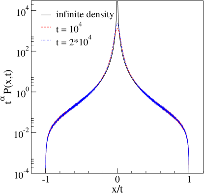
Figure 1: (color online) $t^{\alpha}P(x,t)$ obtained from numerical simulations for the model with uniform velocity distribution, $v\in[-1,1]$. In the long time limit simulations converge to the infinite density Eq. (55). We used function $\psi(\tau)=\alpha\tau^{-(1+\alpha)}$ for $\tau>1$ as the waiting time PDF. The parameters are $\alpha=3/2$, $A=\alpha|\Gamma(-\alpha)|$, and $\langle\tau\rangle=1$. Two histograms for $t=10^{4}$ and $2\times 10^{4}$ were sampled over $N=10^{10}$ realizations.

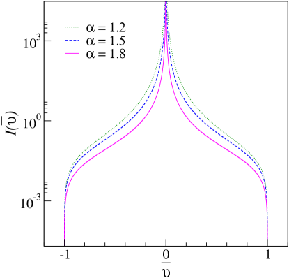
Figure 2: (color online) Infinite densities for the model with uniform velocity distribution, $v\in[-1,1]$, Eq. (55) in the main text. $A=\alpha|\Gamma(-\alpha)|$ and $\langle\tau\rangle=1$.

VI.1 Graphical Examples

In Fig. 1 we plot $t^{\alpha}P(x,t)$ obtained from finite time simulations of the Lévy walk, versus $x/t$. According to the theory, in the limit $t\to\infty$ this plot will approach the infinite density, Eq. (38). Such a behavior is indeed confirmed with the simulations in the figure. This implies that with a finite time simulation or experiment, which measures the density of particles, we can estimate the infinite density. In the figure we see that data collapse (for finite time) is performing better for large $x/t$, and convergence for small values of $x/t$ is slow. Indeed, for $x=0$ the density is well described by the Lévy central limit theorem, as we soon explain.

In the right panel in Fig. 3 we demonstrate numerically the relation between the small $\overline{v}$ behavior of ${\cal I}(\overline{v})$ and the anomalous diffusion coefficient $K_{\alpha}$, Eq. (42). Plotting ${\cal I}(\overline{v})/c_{\alpha}K_{\alpha}$ versus $\overline{v}$ we see that in the limit of small $\overline{v}$, various models collapse on one master curve. So with the knowledge of $K_{\alpha}$ and $\alpha$, which as explained in the next section can be determined from data, we can predict the small $\overline{v}$ behavior of the infinite density. As mentioned before, the large $\overline{v}$ behavior of the infinite density, Eq. (44), is sensitive to the shape of the velocity CDF $Q(v)$, hence for large $\overline{v}$ the corresponding curves in the figure depart. This sensitive tool in real experiments may unravel important statistical information on the process.

Practically, though dealing with long time limit solutions, Eq. (60) implies one should analyze the results for the shortest valid measurement times possible to maximize the probability of the region of interest. Thus measurement time must be long, so that asymptotic limit is reached, but not too long such that we can sample the tails of the PDF (similar to many other problems in physics, for example large deviation theory). The estimation of this time scale depends not only on the details of the model, but also on the number of particles undergoing the super-diffusive process, and the detailed problem of estimation of infinite densities from finite amount of data, is left for future work.

In contrast, the center part of the density, discussed in the next section, is described by the generalized central limit theorem, thus it is universal, but does not yield information on $F(v)$. Thus, infinite densities might become important tools in unraveling the origin of anomalous diffusion, a topic which attracted considerable theoretical attention, e.g., PCCP ; Garini ; Soko and ref. therein.

In simulations we reached a high degree of accuracy with extensive simulations and resolved the probabilities of the events at the PDF tails that are six order of magnitudes smaller than of those contributing to the PDF maximum, see the right panel of Fig. 1. The PDFs have been sampled with $N=10^{10}$ realizations. The corresponding simulations were performed on two GPU clusters (each consisting of six $\rm{TESLA~{}K20XM}$ cards) and took $380$ hours. The main reason that we choose such a large number of particles, is to illustrate the theory with maximal possible (at the moment) precision. Single particle experiments in a single cell Naama are conducted with much smaller number of particles, and for that reason it would be interesting to simulate the process for smaller numbers of particles and shorter times, to see if how accurately one may estimate the infinite density. However, in other experiments, like laser cooling of cold atoms Sagi , the number of particles is vast so these limitations are absent.

Remark: Upon inspection of Fig. 3, we realize that the probabilities of the events contributing to the PDF tails are six order of magnitude smaller than those contributing to the plotted PDF maximum. This six order of magnitude difference is related to the choice of scale in the figure, since the infinite density diverges on the origin. For example in the left panel we cut off the divergence on the origin. In reality, experiments are performed for finite times. Hence the infinite density is slowly approached, but never actually reached, in the vicinity of the origin (see Fig. 1). Put differently, we need to sample rare fluctuations, and here sophisticated sampling algorithms could be useful sampling1 ; sampling2 ; sampling3 .

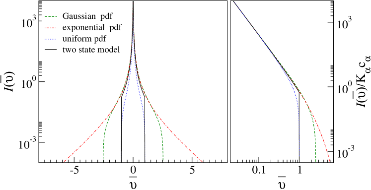
Figure 3: (color online) Infinite densities for different models, see section “Examples” in the main text. The parameters are the same as in Fig. 1. The right panel shows universal behavior of the infinite density in the small $\overline{v}$ limit according to Eq. (43). When the infinite density is rescaled with the anomalous diffusion constant $K_{\alpha}$ times the constant $c_{\alpha}$ these non-normalized densities fall on a master curve. Hence once we record $K_{\alpha}$ and $\alpha$ we can predict the small $\overline{v}$ behavior of ${\cal I}(\overline{v})$. Here $\alpha=3/2$ and $K_{3/2}=(\sqrt{2\pi}/3)\langle|v|^{3/2}\rangle$ and $\langle|v|^{3/2}\rangle=1,2/5,\sqrt{\pi}/4,2^{3/4}/\sqrt{\pi}$ for the two state, uniform, exponential and Gaussian models respectively. Notice the log-log scale on the right panel.

VII The Lévy scaling regime

The key step in our derivation of ${\cal I}\left(\overline{v}\right)$ was an expansion of the Montroll-Weiss equation, Eq. (11), in the small $k,u$ limit while the ratio of $k/u$ is kept fixed. This led to a scaling of the type $x\propto t$. As we showed, such an expansion leads to a non-normalized density ${\cal I}(\overline{v})$, as opposed to the normalization dictated by Eq. (11).

To complete the the large order moments scheme we now consider the expansion of the Montroll-Weiss equation assuming that that $k^{\alpha}/u$ is fixed and $u$ is small, i.e., we consider the long time limit and inspect the PDF around the origin. Such an assumption means that we are looking for a solution with a scaling $x\propto t^{1/\alpha}$. This scaling describes the center part of the PDF $P(x,t)$ only and does address the PDF’s tails. It yields a normalized solution but at a price of a divergent second and all higher moments. Thus, if we wish to calculate the second moment $\langle x^{2}\rangle$, we need to estimate the tails of the $P(x,t)$ and use the infinite density, i.e. perform the fixed $k/u$ expansion. In contrast, if we want to estimate the normalization, or the low order moments $\langle|x|^{q}\rangle$ with $q<\alpha$, we need an estimation of the center part of the PDF, and hence and expansion with $k^{\alpha}/u$ fixed. Such low order moments cannot be estimated with the infinite density because

$$\langle|x|^{q}\rangle=2\int_{0}^{\infty}P(x,t)x^{q}{\rm d}x\neq 2\int_{0}^{\infty}x^{q}t^{-\alpha}{\cal I}\left({x\over t}\right){\rm d}x=\infty$$ (61)

for $0<q<\alpha$, due to the singular behavior of the infinite density at the origin.

To illustrate the above consideration, we take Eq. (14) and expand it assuming that $|u|\ll|kv|\ll 1$ and $k$ is small,

$$P_{\rm cen}(k,u)\sim\frac{1-A_{\tau}\left\langle(-ikv)^{\alpha-1}\left[1-(\alpha-1)\frac{u}{ikv}\right]\right\rangle}{u-A_{\tau}\left\langle(-ikv)^{\alpha}\left[1-\alpha\frac{u}{ikv}\right]\right\rangle}\sim\frac{1}{u-A_{\tau}\left\langle(-ikv)^{\alpha}\right\rangle}.$$ (62)

The subscript “${\rm cen}$” indicates we aim at the center part of $P(x,t)$. The term $\left\langle(-ikv)^{\alpha}\right\rangle$ can further be simplified by recalling the symmetry of $F(v)$,

$$\begin{array}[]{rl}\left\langle(-ikv)^{\alpha}\right\rangle&=|k|^{\alpha}\left\langle|v|^{\alpha}e^{-\frac{i\pi\alpha}{2}\text{ sign}(kv)}\right\rangle\\ \\ &=|k|^{\alpha}\left\langle|v|^{\alpha}\right\rangle\cos{\left(\frac{\pi\alpha}{2}\right)}.\end{array}$$ (63)

By inserting it into Eq. (62) we find

$$P_{\rm cen}(k,u)\sim\frac{1}{u+K_{\alpha}|k|^{\alpha}},$$ (64)

where $K_{\alpha}$ is the anomalous diffusion coefficient, proportional to the moment $\langle|v|^{\alpha}\rangle$ of the PDF $F(v)$, Eq. (42). Thus, here the dynamics is not sensitive to the full shape of the velocity distribution but only to a particular $\alpha$-th moment.

The solution Eq. (64) is well known Bouchaud ; GL ; Review ; ZK ; Carry ; its inverse Laplace transform is

$$P_{{\rm cen}}(k,t)\sim\exp\left(-K_{\alpha}t|k|^{\alpha}\right)\>.$$ (65)

As is well known, the Fourier transform of the symmetrical Lévy density $L_{\alpha}(y)$ is $\exp(-|k|^{\alpha})$, which serves as our working definition of this stable density. Hence by definition, the inverse Fourier transform of Eq. (65) yields a symmetric Lévy stable PDF Bouchaud ; Review ; levy

$$P_{\rm cen}(x,t)\sim{1\over(K_{\alpha}t)^{1/\alpha}}L_{\alpha}\left[{x\over(K_{\alpha}t)^{1/\alpha}}\right]\>.$$ (66)

The Lévy density is normalized, its second moment diverges since for large $x$ the solution has a fat tail $L_{\alpha}(x)\propto|x|^{-(1+\alpha)}$. When $\alpha\to 2$ we approach the Gaussian limit.

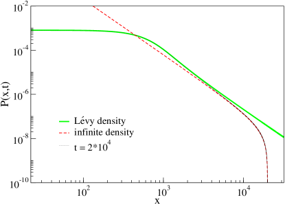
Figure 4: (color online) PDF $P(x,t)$ for the model with uniform velocity distribution, $v\in[-1,1]$, see Fig. 1, plotted together with Lévy distribution and rescaled infinite density. The parameters are the same as in Fig. 1.

One cannot say that either of the two Montroll-Weiss expansions presented so far is the correct expansion, without specifying the observable of interest and the domain in $x$ where one wishes to estimate the density. Thus, if we wish to calculate the second moment $\langle x^{2}\rangle$ from an estimation of the density of particles, we need the infinite density (i.e. the fixed $k/u$ expansion) estimating the tails of the $P(x,t)$. In contrast, if we want to estimate the normalization, or the low order moments $\langle|x|^{q}\rangle$ with $q<\alpha$, we need an estimation of the center part of the packet, Eq. (66).

VIII Infinite and Lévy densities are complementary

As shown in Fig. 4, for long, though finite times the center/tail region of $P(x,t)$ is well approximated by the Lévy/infinite density respectively. We define a crossover position $x_{c}(t)>0$ below/above which the Lévy/infinite densities are valid approximations. The maximum of $P(x,t)$ is clearly on the origin (neglecting possible finite time delta peaks found, for example, for the two state velocity model, since these do not contribute in the $t\to\infty$ limit to the moments of the process). Hence, any estimation for the density for $x\neq 0$ and long times must be smaller than the value of the density on the origin. On the origin

$$P(x,t)|_{x=0}\sim{L_{\alpha}(0)\over(K_{\alpha}t)^{1/\alpha}}\>,$$ (67)

with $L_{\alpha}(0)=\int_{-\infty}^{\infty}\exp(-|k|^{\alpha}){\rm d}k/2\pi=\Gamma(1+\alpha^{-1})/\pi$. Using $P(x,t)\sim{\cal I}(x/t)/t^{\alpha}$ we define $x_{c}$ via the condition

$${{\cal I}\left({x_{c}\over t}\right)\over t^{\alpha}}={L_{\alpha}\left(0\right)\over\left(K_{\alpha}t\right)^{1/\alpha}}\>.$$ (68)

Since the transition to the Lévy regime is found for the small argument behavior of the infinite density we use Eq. (43), ${\cal I}(x_{c}/t)\sim c_{\alpha}K_{\alpha}/|x_{c}/t|^{1+\alpha}$ and after some simple algebra we find

$$x_{c}(t)=\left[{c_{\alpha}\over L_{\alpha}(0)}\right]^{{1\over 1+\alpha}}\left(K_{\alpha}t\right)^{1/\alpha}\>.$$ (69)

Though only a rough estimation for the transition, the important point is to notice that $x_{c}(t)\propto t^{1/\alpha}$. When data for $P(x,t)$ is presented versus the scaled variable $x/t$ (the variable $\overline{v}$) we have a crossover velocity $x_{c}(t)/t\sim t^{(1/\alpha)-1}$ which goes to zero as $t\to\infty$ since $\alpha>1$. Thus, the infinite density becomes a better approximation of $t^{\alpha}P(x,t)$ versus $x/t$ as time is increased, see Fig. 1.

Based on this picture let us calculate the $q$-th moment with $q>\alpha$, being a real number. We divide the spatial integration into two parts and find

$$\langle|x|^{q}\rangle\simeq\underbrace{2\int_{0}^{x_{c}(t)}{L_{\alpha}\left[{x\over\left(K_{\alpha}t\right)^{1/\alpha}}\right]\over\left(K_{\alpha}t\right)^{1/\alpha}}x^{q}{\rm d}x}_{\text{ \mbox{inner L\'{e}vy region}}}+\underbrace{2\int_{x_{c}(t)}^{\infty}{{\cal I}\left({x\over t}\right)\over t^{\alpha}}x^{q}{\rm d}x}_{\text{ outer tail, infinite density region}}\>.$$ (70)

Changing variables according to $y=x/(K_{\alpha}t)^{1/\alpha}$ in the first integral on the right hand side, and to $\overline{v}=x/t$ for the second integral we have

$$\langle|x|^{q}\rangle\simeq 2(K_{\alpha}t)^{q/\alpha}\int_{0}^{x_{c}(t)/(K_{\alpha}t)^{1/\alpha}}L_{\alpha}(y)y^{q}{\rm d}y+2t^{q+1-\alpha}\int_{x_{c}(t)/t}^{\infty}{\cal I}\left(\overline{v}\right)\overline{v}^{q}{\rm d}\overline{v}\>.$$ (71)

In the long time limit, the lower limit of the second integral $x_{c}(t)/t\to 0$ while the upper limit of the first integral is a constant. For $q>\alpha$ the second integral is by far larger than the first, hence we may neglect the inner region

$$\langle|x|^{q}\rangle\sim 2t^{q+1-\alpha}\int_{0}^{\infty}{\cal I}\left(\overline{v}\right)\overline{v}^{q}{\rm d}\overline{v}.$$ (72)

The $\overline{v}^{q}$ in the integrand “cures” the non-integrable infinite density, i.e., the non-integrability arising from the small $\overline{v}$ divergence of ${\cal I}(\overline{v})$, in the sense that the integral is finite when $q>\alpha$. When $q=2n$ in Eq. (72) with a positive integer $n$ we retrive Eqs. (19,59).

In the opposite limit $q<\alpha$ we find the opposite trend, namely now the inner region of the density $P(x,t)$ is important in the estimation of the moments $\langle|x|^{q}\rangle$. To see this we first note that in the intermediate region of $x$, the Lévy and infinite densities are equivalent. The intermediate region are values of $x$ where the density $P(x,t)$ is well approximated by the power law tail of the Lévy density, before the cutoff due the finite velocity, and after the small $x$ region where the Lévy density did not yet settle into a power law behavior. Indeed, there is a relation between the infinite density and the Lévy density since they must match in the intermediate region. Using the known large $y$ behavior $L_{\alpha}(y)\sim c_{\alpha}y^{-(1+\alpha)}$ we obtain

$$t^{\alpha}P_{{\rm cen}}(x,t)\sim c_{\alpha}K_{\alpha}|x/t|^{-(1+\alpha)}\>.$$ (73)

This is exactly the same as the small $\overline{v}=x/t$ behavior of the infinite density, Eq. (43), hence, the two solutions match as they should.

To obtain $\langle|x|^{q}\rangle$ with $q<\alpha$ we define a velocity crossover $v_{c}$ which is of the order of the typical velocity of the problem (a velocity scale of $F(v)$). For $|x|/t<v_{c}$ the density $P(x,t)$ is well approximated by a Lévy density (since in the intermediate region the latter and the infinite density match), while beyond $v_{c}$ we have the infinite density description

$$\langle|x|^{q}\rangle\simeq 2\int_{0}^{v_{c}t}{L_{\alpha}\left[{x\over\left(K_{\alpha}t\right)^{1/\alpha}}\right]\over\left(K_{\alpha}t\right)^{1/\alpha}}x^{q}{\rm d}x+2\int_{v_{c}t}^{\infty}{{\cal I}\left({x\over t}\right)\over t^{\alpha}}x^{q}{\rm d}x\>.$$ (74)

Now when $t\to\infty$ and $q<\alpha$ the contribution from the second integral is negligible and the upper limit of the first integral is taken to infinity, hence, after a change of variables $y=x/(K_{\alpha}t)^{1/\alpha}$, and using the symmetry $L_{\alpha}(y)=L_{\alpha}(-y)$

$$\langle|x|^{q}\rangle\sim\left(K_{\alpha}t\right)^{q\over\alpha}\int_{-\infty}^{\infty}L_{\alpha}(y)|y|^{q}{\rm d}y\>.$$ (75)

We see that moments integrable with respect to the infinite density, i.e. $q>\alpha$ are obtained from the non-normalizable measure. While for an observable which is non-integrable with respect to the infinite density, i.e. $|x|^{q}$ and $q<\alpha$, the Lévy density yields the average and is used in the calculation.

Further mathematical analysis of this behavior is required. An observable like $f(x)=1/(1+\sqrt{|x|})$ is non integrable with respect to the infinite density. The average of $f(x)$ with respect to the Lévy density is finite. Hence the average $\langle f(x)\rangle$ is computed with an integration over the Lévy density. On the other hand consider an observable like $g(x)=|x|^{\alpha+\epsilon}\theta(1-|x|)$ where $\theta(\cdots)$ is the step function and $\epsilon>0$. Now $g(x)$ is integrable with respect to the infinite density but also integrable with respect to the Lévy density. So how do we obtain its average? Do we use the infinite density or the Lévy density? Since $P(x,t)$ is well approximated by the Lévy density in the regions where the function $g(x)$ is not zero, i.e. for $|x|<1$ the Lévy density should be used in the calculation. This example shows that not all averages of observables integrable with respect to the infinite density are obtained from the non-normalized density. One can also construct an observable which is not integrable with respect to the Lévy density neither with respect to the infinite density; e.g., a function that behaves like $h(x)\sim x^{2}$ for large $x$ and $h(x)\sim 1$ for $x\to 0$. A trivial example is $h(x)=1+x^{2}$ since the average of this function is given by both the Lévy density to compute $\langle 1\rangle=1$ and $\langle x^{2}\rangle>>1$ which is found from the infinite density. Hopefully future rigorous work will present a full classification of observables and rules for their calculation. Another approach it to obtain a uniform approximation for $P(x,t)$ based on the Lévy and infinite densities. This approximation which works for all $x$ will be presented elsewhere and it can serve as a tool for calculation of different classes of observables.

VIII.1 Strong Anomalous Diffusion

From Eqs. (72, 75) we find

$$\langle|x|^{q}\rangle\sim\left\{\begin{array}[]{l l}M_{q}^{<}\ t^{q/\alpha},&q<\alpha,\\ &\\ M_{q}^{>}\ t^{q+1-\alpha},&q>\alpha,\end{array}\right.$$ (76)

with amplitudes

$$M_{q}^{<}={\left(K_{\alpha}\right)^{q\over\alpha}\Gamma\left(1-{q\over\alpha}\right)\over\Gamma\left(1-q\right)\cos\left(\pi q/2\right)}$$ (77)

and

$$M_{q}^{>}={2K_{\alpha}c_{\alpha}q\langle|v|^{q}\rangle\over\alpha\left(q-\alpha\right)\left(q-\alpha+1\right)\langle|v|^{\alpha}\rangle}\>.$$ (78)

The amplitudes $M_{q}^{<}$ and $M_{q}^{>}$ diverge as $q\to\alpha$ from above or below, and in that sense the system exhibits a dynamical phase transition. This behavior is shown in Fig. 5 where finite time simulations show a clear peak of the moments amplitudes in the vicinity of $q=\alpha$. The system exhibits strong anomalous diffusion with a bi-linear spectrum of exponents, i.e., $q\nu(q)$ in Eq. (1) is bi-linear. Such a behavior is demonstrated in Fig. 6, where $q\nu(q)$ versus $q$ is plotted using finite time simulations, which indicate that convergence to asymptotic results is within reach Zabu1 . As mentioned in the introduction, this piecewise linear behavior of $q\nu(q)$, is a widely observed behavior.

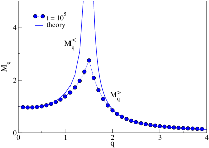
Figure 5: (color online) Moment amplitudes for the uniform model exhibit a critical behavior on $q=\alpha$, in the infinite long time limit these moments diverge as $q\to\alpha$ $(\alpha=3/2$ in this example). Lines correspond to Eqs. (77, 78) in the main text. Dots are the results of sampling with $N=10^{9}$ realizations. Dashed line was obtained by combining together the Lévy distribution and infinite density (see Fig. 4) and gluing them together at the point $x=15000$ remark1 . Parameters are the same as in Fig. 1 with $t=10^{5}$.

IX Discussion

The Lévy walk model exhibits enhanced diffusion where $\langle x^{2}\rangle\propto t^{3-\alpha}$ when $1<\alpha<2$. Such a behavior is faster than diffusive and slower than ballistic. Unlike Gaussian processes with zero mean, the variance $\langle x^{2}\rangle$ is not a sufficient characterization of the motion. Mono scaling solutions $P(x,t)\sim t^{-\xi}g(x/t^{\xi})$, which assume that the density of particles in the long time limit has a single characteristic scale, fail to describe the dual nature of the dynamics which contains both Lévy motion and ballistic elements in it. The density of particles at its center part is described by the symmetric Lévy distribution. If the Lévy central limit theorem is literally taken, it predicts a divergence of the mean square displacement at finite times, i.e., the variance of the stable PDF $L_{\alpha}(x)$ is infinite when $0<\alpha<2$. The tails of the Lévy walk model exhibit ballistic scaling, indeed as well known, the density is cutoff by ballistic flights. In this work we have found the mathematical description of the ballistic elements of the transport. An uncommon physical tool, a non-normalizable density describes the packet of particles. The bi-linear scaling of the moments, i.e., strong anomalous diffusion, means that we have two complementary scaling solutions for the problem. The first describes the center part of the packet and is the well known Lévy stable density with the scaling $x\propto t^{1/\alpha}$. The second scaling solution describes ballistic scaling $x\propto t$ and is given by our rather general formula for the infinite density Eq. (38). The equation exhibits a certain universality in the sense that it does not depend on the full shape of the waiting times PDF. It relates the non-normalized density with three measurable quantities: the velocity distribution of the particles, the anomalous diffusion exponent $\alpha$ and the anomalous diffusion coefficient $K_{\alpha}$.

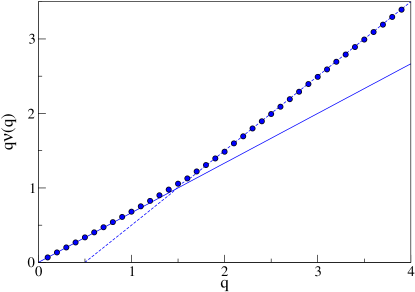
Figure 6: (color online) The spectrum of exponents $q\nu(q)$ versus $q$ exhibits piecewise linear behavior. The finite time simulations (dots, parameters as in Fig. 5), for the uniform model, perfectly agree with theory (lines): for $q<\alpha$ $q\nu(q)=q/\alpha$ otherwise $q\nu(q)=q+1-\alpha$ (see Eq. 76). Here $\alpha=3/2$.

In this paper we have focused on a model with two scalings, namely ballistic $x\propto t$ and Lévy $x\propto t^{1/\alpha}$ motions. In real systems we may have a mixture of other modes of motion. For example, Gal and Weihs Naama measured the spectrum of exponents $q\nu(q)$ and found for large $q$ a linear behavior $q\nu(q)\sim cq$ and $c\simeq 0.8-0.6$ so this motion is slower than ballistic but faster than diffusive. This is probably related to the active transport of the measured polymer embedded in the live cell, namely to the input of energy into the cell. In this direction, one should consider more general models. For example variation of the Lévy walks where waiting times are power law distributed but jump’s lengths scale non-linearly with waiting times, i.e. $x=\sum_{i=0}^{N}v_{i}(\tau_{i})^{\beta}+v_{N}(\tau_{b})^{\beta}$ with $\beta>0,\beta\neq 1$. Work on other regime of parameters is also in progress. We recently investigated the regime $\alpha>2$, where the Gaussian central limit theorem holds, and found that the infinite density concept remains in tact. Thus even a normal process, in the sense that the center part of $P(x,t)$ is described by the Gaussian central limit theorem, its rare fluctuations are related to a non-normalizable measure. It is left for future rigorous work to see if infinite densities describe non-linear dynamical systems, at least those where power law distributions of waiting times between collision events, are known to describe the dynamics Dettman ; Balint .

Our results seem widely applicable. We know that bi-scaling of the spectrum of exponents is a common feature of different systems and strong anomalous diffusion is a well documented phenomena. The Lévy walk dynamics is ubiquitous and has been recorded in many systems. Hence we are convinced that the infinite density concept has a general validity, ranging from dynamics in the cell, motion of tracer particles in non-linear flows, spatial diffusion of cold atoms to name a few. The question of estimation of infinite density from not too large ensembles of particles and finite time experiments is left for future work.

In solid state physics, transport is in many cases characterized as either ballistic or diffusive. The system falls into one of these categories depending on the ratio of the size of the system and mean free path. Here a completely different picture emerges. Depending on the observable, i.e. the order of the moment, the same system exhibits either diffusive or ballistic transport. Observables integrable with respect to the infinite density are ballistic, while observables integrable with respect to the Lévy density exhibit super diffusion. So in these systems the question of what is measured becomes crucial, and one cannot say that the process/system itself falls into a unique category of motion. At-least in our model, bi-scaling means that we have two sets of tools to master, the infinite density being the relatively newer concept which might need more clarifications in future work Large and become a valuable approach in other problems of statistical physics.

X Appendix: $P(k,u)$ for the Lévy walk

In this Appendix we derive the Montroll-Weiss equation (11) relating the Fourier-Laplace transform of $P(x,t)$ with the velocity and waiting time PDFs, $F(v)$ and $\psi(\tau)$ respectively. We denote the position of the particle $x_{N}(t)$ (instead of $x(t)$ used in the text), where $N$ is the random number of collisions and rewrite Eq. (2)

$$x_{N}(t)=\sum_{j=1}^{N}v_{j-1}\tau_{j}+v_{N}\tau_{b}\>.$$ (79)

The standard approach to the problem is an iterative approach, namely to relate the probability density of finding the particle at $x$ after $j$ collision events, with the density conditioned on $j+1$ collisions, e.g. Carry . Using the renewal assumption one gets convolution integrals, and that leads to Eq. (11). We will use a slightly different method, to avoid a complete repeat of previous derivations, our approach is inspired by the renewal theory in GL .

The PDF of the position of the particles, all starting on the origin $x=0$, at time $t$ is

$$P(x,t)=\sum_{N=0}^{\infty}{\langle\Theta(t-t_{N})\Theta(t_{N+1}-t)\delta[x-x_{N}(t)]\rangle}\>,$$ (80)

where $\delta(\cdots)$ is the Dirac delta function. Here $t_{N}$ denotes the time of the $N$-th collision event $t_{N}=\sum_{i=1}^{N}\tau_{i}$. The multiplication of the two step functions in Eq. (80), i.e., the $\Theta(t-t_{N})\Theta(t_{N+1}-t)$ term, gives the condition $t_{N}<t<t_{N+1}$, for the measurement time $t$. The summation over $N$ in Eq. (80) is a sum over all possible number of collision events. Transforming $P(x,t)$ into the Fourier-Laplace domain, using Eq. (10), we obtain

$$P(k,u)=\sum_{N=0}^{\infty}{\left\langle\int_{t_{N}}^{t_{N+1}}{\text{exp}({ikx_{N}(t)-ut}){\rm d}t}\right\rangle}\>.$$ (81)

The averages here are with respect to the velocity and the waiting time distributions. Inserting Eq. (79) in Eq. (81) we perform the time integral on the right hand side of Eq. (81) using $t_{N+1}-t_{N}=\tau_{N+1}$ and $\tau_{b}=t-t_{N}$

$$\begin{array}[]{rl}P(k,u)&=\sum_{N=0}^{\infty}{\left\langle\frac{1-\text{exp}[{(ikv_{N}-u)\tau_{N+1}}]}{u-ikv_{N}}{\prod_{j=1}^{N}\text{exp}[{(ikv_{j-1}-u)\tau_{j}}]}\right\rangle}\\ \\ &=\left\langle\frac{1-\text{exp}[{(ikv_{0}-u)\tau_{1}}]}{u-ikv_{0}}\right\rangle+\sum_{N=1}^{\infty}{\left\langle\frac{1-\text{exp}[{(ikv_{N}-u)\tau_{N+1}}]}{u-ikv_{N}}\prod_{j=1}^{N}\text{exp}[{(ikv_{j-1}-u)\tau_{j}}]\right\rangle}\>.\end{array}$$ (82)

Here we separated the case of zero collisions $N=0$ from $N\geq 1$. Because the velocities and waiting times are mutually independent, each separately being independent identically distributed random variables, we can perform the averaging. With the Laplace transform Eq. (6), $\hat{\psi}(u)=\left\langle e^{-u\tau}\right\rangle$, we use

$$\langle\Pi_{j=1}^{N}\exp[(ikv_{j-1}-u)\tau_{j}]\rangle=\langle\hat{\psi}(u-ikv)\rangle^{N}\>,$$ (83)

where the remaining averaging on the right hand side is with respect to the velocity PDF only $\langle\cdots\rangle=\int_{-\infty}^{\infty}{\rm d}v\cdots F(v)$. Hence from Eq. (82) we find

$$P(k,u)=\left\langle\frac{1-\text{exp}[{(ikv-u)\tau}]}{u-ikv}\right\rangle\sum_{N=0}^{\infty}{\left\langle\text{exp}[{(ikv-u)\tau}]\right\rangle^{N}}=\left\langle\frac{1-\hat{\psi}(u-ikv)}{u-ikv}\right\rangle\sum_{N=0}^{\infty}{\left\langle\hat{\psi}(u-ikv)\right\rangle^{N}}\>.$$ (84)

This geometric series sum is convergent and yields the known Montroll-Weiss equation, Eq. (11).

References

- (1) A. Pikovsky, Phys. Rev. A 43, 3146 (1991).
- (2) P. Castiglione, A. Mazzino, P. Muratore-Ginanneschi, and A. Vulpiani, Physica D 134, 75 (1999).
- (3) J. P. Bouchaud and P. Le Doussal, J. Stat. Phys. 41, 225 (1985).
- (4) A. Zacherl, T. Geisel, J. Nierwetberg, and G. Radons, Phys. Lett. A 114, 317 (1986).
- (5) J. P. Bouchaud and A. Georges, Phys. Rep. 195, 127 (1990).
- (6) R. Artuso and G. Cristadoro, Phys. Rev. Lett. 90, 244101 (2003).
- (7) D. N. Armstead, B. R. Hunt, and E. Ott, Phys. Rev. E. 67, 021110 (2003).
- (8) D. P. Sanders and H. Larralde, Phys. Rev. E, 73, 026205 (2006). Here the authors demonstrate that even for a model of finite horizon, high order moments behave ballistically. This is due to a non-trivial correlation between collision events, hence the infinite horizon condition is not a a necessary condition for our discussion.
- (9) M. Courbage, M. Edelman, S. M. Saberi Fathi, and G. M. Zaslavsky, Phys. Rev. E. 77, 036203 (2008).
- (10) T. Geisel, A. Zacherl, and G. Radons, Phys. Rev. Lett. 59, 2503 (1987).
- (11) J. Klafter and G. Zumofen, Phys. Rev. E 49, 4873 (1994).
- (12) P. Levitz, Europhys. Lett. 39, 593 (1997).
- (13) E. Barkai, V. Fleurov, and J. Klafter Phys. Rev. E 61 164 (2000).
- (14) P. Barthelemy, J. Bertolotti, and D. S. Wiersma, Nature 453, 495 (2008).
- (15) N. Gal and D. Weihs, Phys. Rev. E 81, 020903(R) (2010).
- (16) K. H. Andersen, P. Castiglione, A. Mazzino, and A. Vulpiani, Eur. Phys. J. B 18, 447 (2000).
- (17) C. Godreche and J. M. Luck, J. Stat. Phys. 104, 489 (2001).
- (18) M. Schmiedeberg, V. Yu. Zaburdaev, and H. Stark, J. Stat. Mech.: Theory and Exp. (2009) P12020; deviations from biscaling are visible (Fig. 4, therein), possibly originating from finite time effects.
- (19) R. Burioni, L. Caniparoli and A. Vezzani, Phys. Rev. E 81, 060101 (2011).
- (20) R. Burioni, G. Gradenigo, A. Sarracino, A. Vezzani, and A. Vulpiani, J. Stat. Mech.: Theory and Exp., P09022(2013).
- (21) P. Bernabo, R. Burioni, S. Lepri, and A. Vezzani arXiv:1404.5878 [cond-mat.stat-mech] (2014)
- (22) B. A. Carreras, V. E. Lynch, D. E. Newman, and G. M. Zaslavsky, Phys. Rev. E 60, 4770 (1999).
- (23) D.A. Kessler and E. Barkai, Phys. Rev. Lett. 105, 120602 (2010).
- (24) A. Dechant and E. Lutz, Phys. Rev. Lett. 108, 230601 (2012).
- (25) P. de Anna, T. Le Borgne, M. Dentz, A. M. Tartakovsky, D. Bolster, and P. Davy, Phys. Rev. Lett. 110, 184502 (2013).
- (26) R. Metzler and J. Klafter, Phys. Rep. 339, 1 (2000).
- (27) P. Siegle, I. Goychuk, and P. Hänggi, Phys. Rev. Lett. 105, 100602 (2010); P. Siegle, I. Goychuk, and P. Hänggi, EPL 93, 20002 (2011). Linear generalized Langevin equations with colored Gaussian noise exhibit Gaussian non-Markovian anomalous diffusion; it is still left to be shown if external non-linear fields may induce strong anomalous diffusion.
- (28) P. Lévy, Théorie de l’addition des variables aléatoires (Gauthiers-Villars, Paris, 1937).
- (29) M. F. Shlesinger, B. J. West, and J. Klafter, Phys. Rev. Lett. 58, 1100 (1987).
- (30) J. Klafter, A. Blumen, and M. F. Shlesinger, Phys. Rev. A 35, 3081 (1987).
- (31) J. Klafter, M. F. Shlesinger, and G. Zumofen, Phys. Today 49 (2), 33 (1996).
- (32) G. Zumofen and J. Klafter, Phys. Rev. E 47, 851 (1993).
- (33) G. Cristadoro, T. Gilbert, M, Lenci, and D. P. Sanders arXiv:1407.0227 [cond-mat.stat-mech]
- (34) A. Rebenshtok, S. Denisov, P. Hänggi, and E. Barkai Phys. Rev. Lett. 112, 110601 (2014).
- (35) M. Thaler, Israel J. Math. 46, 67 (1983).
- (36) J. Aaronson, An Introduction to Infinite Ergodic Theory (Am. Math.l Soc., Providence, 1997).
- (37) M. Thaler and R. Zweimüller, Probability theory and related fields 135, 15 (2006).
- (38) N. Korabel and E. Barkai, Phys. Rev. Lett. 102, 050601 (2009).
- (39) T. Akimoto and T. Miyaguchi, Phys. Rev. E. 82, 030102(R) (2010).
- (40) T. Akimoto, Phys. Rev. Lett. 108, 164101 (2012). Here, the infinite density is considered for a reduced map and in this sense the system is finite.
- (41) The Lévy walk in its original schematization was equipped with a constant velocity of the motion, , i.e., Shles . Here we consider a generalization of the original model, so-called ’random walks with random velocities’, where the velocity of the ballistic epochs is a random variable itself, see E. Barkai and J. Klafter, in Chaos, Kinetics and Non- linear Dynamics in Fluids and Plasmas, ed. by S. Benkadda and G. M. Zaslavsky, Lect. Not. in Phys., v. 511, pp. 373-393 (Springer Berlin Heidelberg, 1998). Note that we use PDFs that are symmetric and their moments are finite. Thus we remain in the domain of Levy walks, see also V. Zaburdaev, M. Schmiedeberg, and H. Stark, Phys. Rev. E 78, 011119 (2008).
- (42) N. Korabel and E. Barkai, Phys. Rev. Lett. 108, 060604 (2012).
- (43) N. Korabel, and E. Barkai J. of Stat. Mech.: Theory and Exp. P08010 (2013).
- (44) E. Lutz and F. Renzoni, Nature Physics 9, 615 (2013).
- (45) P. C. Holz, A. Dechant, and E. Lutz, arXiv:1310.3425 [cond-mat.stat-mech] (2013).
- (46) A. Rebenshtok, E. Barkai, Phys. Rev. Lett. 99, 210601 (2007).
- (47) A. Rebenshtok, E. Barkai, J. Stat. Phys. 133, 565 (2008).
- (48) E. Barkai and J. Klafter, in Proceedings of a workshop held in Carry-Le-Rouet, June 1997, S. Benkadda and G. M. Zaslavsky Editors Springer (Berlin).
- (49) M. Kotulski, J. Stat. Phys. 81, 777 (1995).
- (50) H. Scher, and M. Lax, Phys. Rev. B 7, 4491 (1973).
- (51) E. Barkai, Chem. Phys. 284, 13 (2002).
- (52) R. Kutner, Chem. Phys. 284, 481 (2002).
- (53) M. Magdziarz, W. Szczotka, P. Zebrowski, J. Stat. Phys. 147, 74 (2012).
- (54) T. H. Solomon, E. R. Weeks, and H. L. Swinney, Phys. Rev. Lett. 71, 3975 (1993).
- (55) A. Ott, J. P. Bouchaud, D. Langevin, and W. Urbach, Phys. Rev. Lett. 65, 2201 (1990).
- (56) Y. Jung, E. Barkai, and R. Silbey, Chem. Phys. 284, 181 (2002).
- (57) G. Margolin and E. Barkai, Phys. Rev. Lett. 94, 080601 (2005).
- (58) G. Margolin, V. Protasenko, M. Kuno, and E. Barkai, J. Phys. Chem. B 110, 19053 (2006).
- (59) F. D. Stefani, J. P. Hoogenboom, and E. Barkai, Physics Today 62 (2), 34 (2009).
- (60) Y. Sagi, M. Brook, I. Almog, and N. Davidson, Phys. Rev. Lett. 108, 093002 (2012).
- (61) D. A. Kessler and E. Barkai, Phys. Rev. Lett. 108, 230602 (2012).
- (62) O. Benichou, C. Loverdo, M. Moreau, and R. Voituriez, Rev. Mod. Phys. 83 81 (2011).
- (63) V. Zaburdaev, S. Denisov, and P. Hänggi, Phys. Rev. Lett. 109, 069903 (2012); V. Zaburdaev, S. Denisov, and P. Hänggi, Phys. Rev. Lett. 110, 170604 (2013).
- (64) A. Figueiredo, T. M. Rocha, M. A. Amato, Z. T. Jr. Oliveira, and R. Matsushita Phys. Rev. E 89, 022106 (2014).
- (65) C. D. Mendl and H. Spohn, Phys. Rev. E 90, 012147 (2014); S. G. Das, A. Dhar, K. Saito, C. B. Mendl, and H. Spohn, Phys. Rev. E 90, 012124 (2014).
- (66) G. Zimbardo, S. Perri, P. Pommois, and P. Veltri, Adv. Space Res. 49, 1633 (2012); G. Zimbardo and S. Perri, Astrophys. J. 778, 35 (2013).
- (67) S. Burov, J. H. Jeon, R. Metzler, and E. Barkai Phys. Chem. Chem. Phys., 13, 1800 (2011).
- (68) E. Barkai, Y. Garini, and R. Metzler, Phys. Today 65(8), 29 (2012).
- (69) F. Thiel, F. Flegel, and I. M. Sokolov, Phys. Rev. Lett. 111, 010601 (2013).
- (70) J. A. Bucklew, Introduction to Rare Event Simulations (Springer Series in Statistics, Springer, NY, 2004).
- (71) J. Tailleur and J. Kurchan, Nature Phys. 3, 203 (2007).
- (72) J. C. Leitão, J. M. Viana Parente Lopes, and E. G. Altmann, Phys. Rev. Lett. 110, 220601 (2013).
- (73) In Fig. 4 and hence the position where the two solutions overlap is roughly while in Fig. 5 hence this point is shifted towards .
- (74) C. P. Dettmann, arXiv:1402.7010v1 (2014)
- (75) P. Balint, N. Chernov, and D. Dolgopyat (preprint) http://www2.math.umd.edu/ dolgop/CuspCLT-3.pdf
- (76) Large deviation theory deals with remote tails of distribution functions, for example with the classical problem of summation of independent random variable with a common PDF. In this example large deviations theory contains the Gaussian central limit theorem and extends it to the regime of large fluctuations Hugo . It is still left to be seen if large deviations theories can be used to obtain infinite densities for the Lévy walk problem.
- (77) H. Touchete, Phys. Rep. 478, 1 (2009).