Analytic approach to the edge state of the Kane-Mele Model

Abstract

We investigate the edge state of a two-dimensional topological insulator based on the Kane-Mele model. Using complex wave numbers of the Bloch wave function, we derive an analytical expression for the edge state localized near the edge of a semi-infinite honeycomb lattice with a straight edge. For the comparison of the edge type effects, two types of the edges are considered in this calculation; one is a zigzag edge and the other is an armchair edge. The complex wave numbers and the boundary condition give the analytic equations for the energies and the wave functions of the edge states. The numerical solutions of the equations reveal the intriguing spatial behaviors of the edge state. We define an edge-state width for analyzing the spatial variation of the edge-state wave function. Our results show that the edge-state width can be easily controlled by a couple of parameters such as the spin-orbit coupling and the sublattice potential. The parameter dependences of the edge-state width show substantial differences depending on the edge types. These demonstrate that, even if the edge states are protected by the topological property of the bulk, their detailed properties are still discriminated by their edges. This edge dependence can be crucial in manufacturing small-sized devices since the length scale of the edge state is highly subject to the edges.

I Introduction

Since the Hall coefficient of the integer quantum Hall effect (IQHE) was known to be described with the topological index,Thouless et al. (1982) the topological quantum state has become one of the main branches in condensed matter physics. Due to the different topological nature of this state, there should exist a gapless mode at the boundary or at the interface even if the bulk state is energetically gapped. There have been lots of efforts to find the similar topological states without a magnetic field. Murakami, Nagaosa, and Zhang found that spin-orbit coupling (SOC) can play the role of the magnetic field in IQHE, and dubbed it as a quantum spin Hall effect (QSHE).Murakami et al. (2003) Kane and Mele suggested a specific model Hamiltonian which shows QSHE.Kane and Mele (2005a, b) Soon after that, Bernevig et al.Bernevig et al. (2006); Bernevig and Zhang (2006) showed that QSHE can be realized in two-dimensional HgTe/CdTe quantum well, and it was confirmed by experiments.König et al. (2007, 2008) The system showing QSHE is also dubbed as a topological insulator (TI) after these works were extended to three-dimensional (3D) materials.Moore and Balents (2007); Fu et al. (2007) The 3D TIs are also confirmed by angle resolved photoemission spectroscopy (ARPES) experiments in Bi_xSb_1-x,Hsieh et al. (2008) Bi₂Se₃,Xia et al. (2009) and Bi₂Te₃.Chen et al. (2009); Hsieh et al. (2009) Consistent results are also yielded by the scanning tunneling microscope (STM) measurements with Bi_1-xSb_xRoushan et al. (2009) and Bi₂Te₃.Alpichshev et al. (2010)

A series of the successes in the TI now open a new route to the novel phases such as Weyl semi-metal and Majorana fermion state.Wan et al. (2011) The interests in this area are also extended to the application-related science such as quantum computing science and spintronics due to the topologically protected surface state and its spin chirality from the time-reversal symmetry.

Despite the success of the ARPES and the STM experiments, the transport experiments of the TI are not so successful to show the metallic surface state. Current TIs are mostly naturally doped or have imperfections in the bulk. This generates residual bulk carriers which prevent the surface current from being detected separately. One of the efforts to reduce the residual carriers is to decrease the thickness of the sample. However, the thickness-dependent experiments show a gap opening when the film is thin enough to cause the overlap between the wave functions on the two opposite surfaces.Zhang et al. (2010) To prevent the overlap of the edge states, we need to control the spatial variation of the edge state in the bulk. Especially, this spatial dependence of the edge-state wave function can be crucial when we consider a small system as in the device manufacturing with TIs.

In this paper, we develop an analytic approach to the Kane-Mele model for the microscopic understanding of the surface state of the TI. Especially, we focus on the spatial profiles of the edge state in the bulk region. First, in Sec. II, we extend the analytic approach for the edge-state wave function developed by König et al. König et al. (2008) and Wang et al. Wang et al. (2009) to the Kane-Mele model. The effect of the edge type is also investigated by considering two typical types of the edge in the honeycomb lattice; an armchair (AC) edge and a zigzag (ZZ) edge. Therefore, we derive two sets of self-consistent equations for the two edges, respectively. In Sec. III, we solve the self-consistent equations numerically, but we also derive an analytical expression for the special case such as $k=\pi$ for the ZZ edge or the case without the sublattice potential, $\lambda_{v}=0$. These results show significant distictions between the systems with the different edges. In this section, we focus on the effect of the internal and the external parameters on the energy dispersion of the edge state, and how the effects are different depending on the edge. The profiles of the edge-state wave function will be discussed in Sec. IV. The spatial properties of the edge state will be discussed by defining the width of the edge state which shows the length scale of the wave function decaying into the bulk. The parameter-dependent edge-state width will be discussed further for the controlling of the edge-state gap in a finite sized system in Sec. V. Finally, we will summarize the results in Sec. VI.

II Self-consistent equation for Kane-Mele model in semi-infinite lattice

In this section we will derive the self-consistent equations for the edge state of Kane-Mele (KM) model in the semi-infinite lattice. First, we construct the Harper’s equationHarper (1955) which describes the wave function in real space in the direction normal to the edge. We consider complex momenta of the Bloch wave function in the direction normal to the edge, since the translational symmetry is broken in that direction. The complex momentum gives the decaying wave function of the edge state. Next, the Harper’s equation yields the effective Hamiltonian for the edge state by using the decaying wave function. Finally, we consider boundary conditions of the edge state, deriving a complete set of equations for the edge-state energy dispersion and the decaying factors of the edge state.

We start from the Kane-Mele modelKane and Mele (2005a, b) which is the tight-binding model with a spin-orbit interaction in a honeycomb lattice.

$$H = -t\sum_{\langle i,j\rangle\sigma}c_{i\sigma}^{\dagger}c_{j\sigma}+i\lambda_{SO}\!\!\!\!\sum_{\langle\langle i,j\rangle\rangle\alpha,\beta}\nu_{ij}\sigma_{\alpha\beta}^{z}c_{i\alpha}^{\dagger}c_{j\beta}$$ (1)

$$+\lambda_{v}\sum_{i\sigma}\zeta_{i}c_{i\sigma}^{\dagger}c_{i\sigma}.$$

Here, the lattice index $i$ and $j$ are the site indices of the honeycomb lattice. $\lambda_{SO}$ is a spin-orbit coupling strength through the next-nearest-neighbor hopping and $\nu_{ij}=\pm 1$ is determined by $\nu_{ij}=\frac{2}{\sqrt{3}}(\mathbf{d}_{1}\times\mathbf{d}_{2})$ where $\mathbf{d}_{1,2}$ are the adjecent two vectors denoting the two nearest-neighbor bonds connecting the next-nearest-neighbor sites. $\sigma^{z}$ is the $z$ component of Pauli matrix, and $\lambda_{v}$ is the sub-lattice potential with $\zeta_{i}=\pm 1$. In the momentum space, the Hamiltonian can be written as

$$H=4\lambda_{SO}\sin q_{x}(\cos q_{x}-\cos q_{y})\Gamma^{15}-\lambda_{v}\Gamma^{2}$$

$$-t\left(2\cos q_{x}+\cos q_{y}\right)\Gamma^{1}-t\sin q_{y}\Gamma^{12}$$ (2)

where $q_{x}=\frac{k_{x}}{2}$, and $q_{y}=\frac{\sqrt{3}}{2}k_{y}$. Here, $\Gamma^{ab}$ and $\Gamma^{a}$ are Dirac matrices shown in Table 1. The energy spectrum can be acquired by diagonalizing the Hamiltonian (2).

$$E_{{\bf q}\sigma}^{2}=\left\{4\lambda_{SO}\sin q_{x}\left(\cos q_{x}-\cos q_{y}\right)-\sigma\lambda_{v}\right\}^{2}$$

$$+t^{2}\left\{1+4\cos^{2}q_{x}+4\cos q_{x}\cos q_{y}\right\}$$ (3)

which gives the bulk energy gap $|3\sqrt{3}\lambda_{SO}\pm\lambda_{v}|$ at $K$ and $K^{\prime}$ in the Brillouin zone of the honeycomb lattice. The $\pm$ sign in the gap depends on the position $K$, $K^{\prime}$ and electron spin. Although both $\lambda_{SO}$ and $\lambda_{v}$ can generate a bulk gap separately, they give topologically different characters to the gap; The $\lambda_{SO}$ gives a topologically non-trivial gap and the $\lambda_{v}$ does a trivial gap. Therefore, when we consider the two parameters at the same time, they compete with each other, and the system can be gapless with a proper ratio of the parameters. Actually, the system has a transition between the topologically trivial state to the non-trivial state when $\lambda_{v}=3\sqrt{3}\lambda_{SO}$. If the system becomes the topologically non-trivial state, it has a gapless edge state on its edge. To investigate the edge state, we need to set an edge in the system. In this work, we will consider two typical edges of a honeycomb lattice; ZZ and AC edges.

$\Gamma^{1}$	$\Gamma^{2}$	$\Gamma^{3}$	$\Gamma^{4}$	$\Gamma^{5}$
$\tau^{x}\otimes I$	$\tau^{z}\otimes I$	$\tau^{y}\otimes\sigma^{x}$	$\tau^{y}\otimes\sigma^{y}$	$\tau^{y}\otimes\sigma^{z}$
$\Gamma^{ab}=\left[\Gamma^{a},\Gamma^{b}\right]/(2i)$

Table 1: Dirac matrices where $\tau$ and $\sigma$ are the Pauli matrices represented in the sublattice space and the spin space, respectively. The operator $\otimes$ is the Kronecker matrix product.

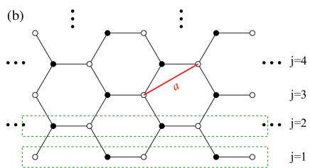
Figure 1: The semi-infinite honeycomb lattice of a lattice constant $a$ with an AC edge. Here, $j$ is a real-space row index in $y$-direction perpendicular to the edge.

II.1 Semi-infinite lattice with an armchair edge

II.1.1 Harper’s equation

As shown in Figure 1, we first consider a semi-infinite lattice which covers the upper-half region ($y>0$) in two-dimensional space and has an AC edge along $x$-axis. In this case, the Hamiltonian (1) can be written in the momentum $k$ in $x$-direction and in the real space lattice index $j$ in $y$-direction. Then the Hamiltonian can be written as

$$H = \sum_{qj}\left(\Psi_{qj}^{\dagger}\hat{M}_{AC}\Psi_{qj}+\Psi_{qj+1}^{\dagger}\hat{T}_{AC}\Psi_{qj}+\Psi_{qj}^{\dagger}\hat{T}_{AC}^{\dagger}\Psi_{qj+1}\right.$$ (4)

$$\left.+\Psi_{qj+2}^{\dagger}\hat{T}^{\prime}_{AC}\Psi_{qj}+\Psi_{qj}^{\dagger}\hat{T}^{\prime\dagger}_{AC}\Psi_{qj+2}\right)$$

where

$$\hat{M}_{AC} = -\lambda_{v}\Gamma^{2}-t\Gamma^{1},$$ (5)

$$\hat{T}_{AC} = 2i\lambda_{SO}\cos q~{}\Gamma^{15}-t\cos q~{}\Gamma^{1}-t\sin q~{}\Gamma^{12},$$ (6)

$$\hat{T}^{\prime}_{AC} = -i\lambda_{SO}\Gamma^{15},$$ (7)

and $q$ is defined as $q=\frac{\sqrt{3}}{2}k$. Now, we can construct the Harper’s equation for the two-dimensional wave function $\Psi_{qj}$ in the following forms,

$$E_{q}\Psi_{qj} = \hat{M}_{AC}\Psi_{qj}+\hat{T}_{AC}\Psi_{qj-1}+\hat{T}_{AC}^{\dagger}\Psi_{qj+1}$$ (8)

$$+\hat{T}^{\prime}_{AC}\Psi_{qj-2}+\hat{T}_{AC}^{\prime\dagger}\Psi_{qj+2},$$

where $E_{q}$ is the energy eigenvalue of the Hamiltonian (4) for the momentum $q$.

II.1.2 Effective Hamiltonian for the edge state

Now, we allow a complex momentum $i\kappa$ for the Bloch wave function in $y$-direction,König et al. (2008); Wang et al. (2009) which can provide a solution to the system with a boundary. The complex momentum eventually makes the wave function decay as it gets into the bulk. Therefore, we can simplify the $j$ dependence of the wave function by using the complex momentum $\kappa$ as the following form

$$\Psi_{qj}=e^{-\kappa(j-1)}\Psi_{q}.$$ (9)

Here, the complex momentum $\kappa$ means the decaying factor of the wave function and it is generally a complex number whose real part is positive for the current boundary condition. The effective Hamiltonian for the edge state can be written with the decaying wave function as

$$E_{q}\Psi_{q}=\hat{H}_{AC}\Psi_{q},$$ (10)

where

$$\hat{H}_{AC}=\hat{M}_{AC}+e^{\kappa}\hat{T}_{AC}+e^{-\kappa}\hat{T}_{AC}^{\dagger}+e^{2\kappa}\hat{T}^{\prime}_{AC}+e^{-2\kappa}\hat{T}_{AC}^{\prime\dagger}.$$ (11)

The explicit matrix form of the effective Hamiltonian for spin $\sigma$ is

$$\hat{H}_{AC}^{\mbox{\scriptsize edge}}=\left[\begin{array}[]{cc}4i\sigma\lambda_{SO}\sinh\kappa\left(\cosh\kappa-\cos q\right)-\sigma\lambda_{v}&-t\left(1+2e^{-iq}\cosh\kappa\right)\\ -t\left(1+2e^{iq}\cosh\kappa\right)&-4i\sigma\lambda_{SO}\sinh\kappa\left(\cosh\kappa-\cos q\right)+\sigma\lambda_{v}\end{array}\right].$$ (12)

From this Hamiltonian, we can get the following eigenvalue equation,

$$E_{q}^{2}=\left\{4i\lambda_{SO}\sinh\kappa\left(\cosh\kappa-\cos q\right)-\sigma\lambda_{v}\right\}^{2}+t^{2}\left\{1+4\cos q\cosh\kappa+4\cosh^{2}\kappa\right\}.$$ (13)

For a given momentum $q$ and energy $E_{q}$, this eigenvalue equation always yields four solutions for the decaying factor, $\kappa$. Thus, with this equation only, we cannot determine the energy dispersion of the edge state, that is, the $q$-dependence of $E_{q}$. For the complete set of equations, we should also consider boundary conditions for the edge-state energy dispersion, which we will derive in the following section.

II.1.3 Boundary condition of the edge state

Let $\kappa_{\nu}$ is the $\nu$-th solution of the eigenvalue equation (13) for a given $q$ and a given energy $E_{q}$. Then the eigenvector for the value of $q$, the energy $E_{q}$, and its solution $\kappa_{\nu}$ can be written as

$$\Phi_{\nu\sigma}^{AC}(q)=\left[\begin{array}[]{c}t\left(1+2e^{iq}\cosh\kappa_{\nu}\right)\\ 4i\sigma\lambda\sinh\kappa_{\nu}\!\left(\cosh\kappa_{\nu}\!-\!\cos q\right)\!-\!\lambda_{v}\!-\!E_{q}\end{array}\right].$$ (14)

Here, $\nu(=1,\cdots,4)$ is an index of the solutions. The general solution, satisfying $\lim_{j\rightarrow\infty}\Psi_{q}=0$, can be written as a linear combination of the eigenvectors.

$$\Psi_{q\sigma}(j)=\sum_{\nu}a_{q\nu}e^{-\kappa_{\nu}(j-1)}\Phi_{\nu\sigma}^{AC}(q),$$ (15)

where $a_{q\nu}$s are arbitrary constants and should be determined by the boundary condition of the system. Now the boundary condition requires $\Psi_{k}(j\leq 0)=0$. From the Harper equation (8), it can be shown that the boundary condition requires the following condition,

$$\Psi_{q}(j=0)=\Psi_{q}(j=-1)=0,$$ (16)

since the Haper’s equation (8) contains the coupling between $\Psi_{k}(j)$ and $\Psi_{k}(j+2)$.

$$\left[\begin{array}[]{cccc}\Phi_{q1\sigma}^{AC}&\Phi_{q2\sigma}^{AC}&\Phi_{q3\sigma}^{AC}&\Phi_{q4\sigma}^{AC}\\ e^{-\kappa_{1}}\Phi_{q1\sigma}^{AC}&e^{-\kappa_{2}}\Phi_{q2\sigma}^{AC}&e^{-\kappa_{3}}\Phi_{q3\sigma}^{AC}&e^{-\kappa_{4}}\Phi_{q4\sigma}^{AC}\end{array}\right]\left[\begin{array}[]{c}a_{q1}\\ a_{q2}\\ a_{q3}\\ a_{q4}\end{array}\right]=0$$ (17)

To have a non-trivial solution for $a_{q\nu}$ we should have

$$\left|\begin{array}[]{cccc}\Phi_{q1\sigma}^{AC}&\Phi_{q2\sigma}^{AC}&\Phi_{q3\sigma}^{AC}&\Phi_{q4\sigma}^{AC}\\ e^{-\kappa_{1}}\Phi_{q1\sigma}^{AC}&e^{-\kappa_{2}}\Phi_{q2\sigma}^{AC}&e^{-\kappa_{3}}\Phi_{q3\sigma}^{AC}&e^{-\kappa_{4}}\Phi_{q4\sigma}^{AC}\end{array}\right|=0.$$ (18)

The eigenvalue equation (13) and the boundary condition (18) provide a complete set of equations for the edge-state energy dispersion and the decaying factors of the edge state. The solutions from the coupled equations can be obtained numerically by an iterative method described in Sec. III and the obtained solutions are presented and analyzed in Secs. III and IV.

Figure 2: The semi-infinite honeycomb lattice of a lattice constant $a$ with a ZZ edge. Here, $j$ is a real-space row index in $y$ direction perpendicular to the edge.

II.2 Semi-infinite lattice with a zigzag boundary

For the zigzag boundary, we already derived the equations for the energy and the wave function in our previous workDoh and Jeon (2013). In this section, we will just summarize the derivation with the new notations in this paper. Based on the semi-infinite lattice as shown in Figure 2 the Hamiltonian with the momentum $k$ in $x$-direction and real space index $j$ in $y$-direction can be written as

$$H=\sum_{qj}\left(\Psi_{qj}^{\dagger}\hat{M}_{ZZ}\Psi_{qj}+\Psi_{qj+1}^{\dagger}\hat{T}_{ZZ}\Psi_{qj}+\Psi_{qj}^{\dagger}\hat{T}_{ZZ}^{\dagger}\Psi_{qj+1}\right)$$ (19)

where

$$\hat{M}_{ZZ} = 2\lambda_{SO}\sin 2q~{}\Gamma^{15}-2t\cos q~{}\Gamma^{1}-\lambda_{v}\Gamma^{2},$$ (20)

$$\hat{T}_{ZZ} = -2\lambda_{SO}\sin q~{}\Gamma^{15}-t(\Gamma^{1}-i\Gamma^{12}).$$ (21)

Here, $q$ is defined as $q=\frac{k}{2}$ in the parallel direction to the edge. Like the previous section, the Harper’s equation is

$$E_{q}\Psi_{qj}=\hat{M}_{ZZ}\Psi_{qj}+\hat{T}_{ZZ}\Psi_{qj-1}+\hat{T}_{ZZ}^{\dagger}\Psi_{qj+1}.$$ (22)

With the same decaying form of the wave function in (9), the effective Hamiltonian can be written as

$$\hat{H}_{ZZ}=\hat{M}_{ZZ}+e^{\kappa}\hat{T}_{ZZ}+e^{-\kappa}\hat{T}_{ZZ}^{\dagger}.$$ (23)

The explicit form of the Hamiltonian for the electron with spin $\sigma$ is

$$\hat{H}_{ZZ}=\left[\begin{array}[]{cc}4\sigma\lambda_{SO}\sin q\left(\cos q-\cosh\kappa\right)-\sigma\lambda_{v}&-t\left(2\cos q+\cosh\kappa-\sinh\kappa\right)\\ -t\left(2\cos q+\cosh\kappa+\sinh\kappa\right)&-4\sigma\lambda_{SO}\sin q\left(\cos q-\cosh\kappa\right)+\sigma\lambda_{v}\end{array}\right].$$ (24)

From this Hamiltonian, we can get the following eigenvalue equation,

$$E_{q}^{2}=\left\{4\lambda_{SO}\sin q\left(\cos q-\cosh\kappa\right)-\sigma\lambda_{v}\right\}^{2}+t^{2}\left\{4\cos^{2}q+4\cos q\cosh\kappa+1\right\},$$ (25)

which gives two values of $\kappa$ for given $q$ and $E_{q}$. Now, we can write down the following $\nu$-th eigenvector corresponding to the solution $\kappa_{\nu}$,

$$\Phi_{\nu\sigma}^{ZZ}=\left[\begin{array}[]{c}t\left(2\cos q\!+\cosh\kappa_{\nu}+\sinh\kappa_{\nu}\right)\\ 4\sigma\lambda_{SO}\sin q\!\left(\cos q\!-\!\cosh\kappa_{\nu}\right)\!-\!\lambda_{v}\!-\!E_{q}\end{array}\right].$$ (26)

From the Harper’s equation of the ZZ edge (22), it can be shown that the boundary condition can be satisfied by

$$\Psi_{k}(j=0)=0.$$ (27)

This means that the two eigenvectors, $\Phi_{1\sigma}^{ZZ}$ and $\Phi_{2\sigma}^{ZZ}$ should be linearly dependent. Therefore, if we define a $2\times 2$ matrix composed of the two vectors, its determinant should be zero

$$\left|\begin{array}[]{cc}\Phi_{q1\sigma}&\Phi_{q2\sigma}\end{array}\right|=0.$$ (28)

Again we express this boundary condition in terms of the eigenvectors (26) which are also functions of $q$, $E_{q}$, and the decaying factors $\kappa$s. The solution of the two coupled equations for ZZ edge, (25) and (28), will be presented in the following two sections along with those of the AC edge.

Figure 3: The edge-state energy dispersion of the ZZ edge for different parameters of the SOC and the sub-lattice potential. The gray shadowed regions are the bulk energy spectra. The red line is for the spin-up electron, and the blue line for the spin-down electron. The topmost graph is the dispersion of the edge state and the energy spectra of the bulk state without any sublattice potential and the lower two are those with a sublattice potential of $\lambda_{v}=0.1t$ for spin-up and spin-down electrons, respectively.

III Energy spectrum

In this section, we solve the coupled equations, (25) and (28) for the edge-state energy of the ZZ edge, and (13) and (18) for that of the AC edge. The overall results in this section generally agree with the previous numerical results.Kane and Mele (2005a); Ezawa and Nagaosa (2013) Nevertheless, since we deal with a semi-infinite lattice, our results are free of any numerical errors which may come from the small size of the system.

For a given $q$, we solve the coupled equations iteratively by the following steps. First, from the initial value of the energy, we solve the equation of $\kappa$s, (25) for the ZZ edge and (13) for the AC edge. From the solutions, we write down the eigenvectors (26) and (14). Finally, as shown in (28) and (18), we construct the $2\times 2$ matrix ($4\times 4$ matrix) with the two (four) eigenvectors from (26) for the ZZ boundary (from (14) for the AC boundary), and extract the new energy value from its determinant condition. Now the new energy is plugged in the first step and these steps are repeated until the energy is converged.

Figure 3 shows the energy dispersion of the edge state for the ZZ boundary. The bulk energy gap occurs at $k=\frac{2\pi}{3}$ and $\frac{4\pi}{3}$ which correspond to the $K$ and $K^{\prime}$ points of the two-dimensional Brillouin zone of the honeycomb lattice. The dispersion of the edge state crosses the gap and connects the valence band maximum at $K$ and the conduction band minimum at $K^{\prime}$, and vice versa for the opposite spin. Without the sub-lattice potential, the spin-up and spin down dispersions cross at $k=\pi$ and the center of the bulk energy gap. If we expand the self consistent equations (25), (26), and (28) for small $k-\pi$ and $\lambda_{v}=0$, then we get the following expression for the energy near $k=\pi$.

$$E_{k}^{ZZ}\simeq v_{F}^{ZZ}(k-\pi)$$ (29)

where $v_{F}^{ZZ}$ is the Fermi velocity of the half-filled system with $\lambda_{v}=0$.

$$v_{F}^{ZZ}=\pm\frac{6\lambda_{SO}t}{\sqrt{t^{2}+16\lambda_{SO}^{2}}}$$ (30)

Here, the Fermi velocity is linearly proportional to the SOC for small SOC, and its derivation is shown in Appendix A.

For the finite sub-lattice potential, the bulk energy spectrum is asymmetric around $k=\pi$. Especially, one of the bulk gaps at $K$ and $K^{\prime}$ get narrower, and the other gets wider. Therefore, the edge dispersion connecting two band edge at $K$ and $K^{\prime}$, moves vertically. The energy shift at $k=\pi$ are proportional to $\lambda_{v}$ as derived in our previous workDoh and Jeon (2013)

$$E_{\pi}^{ZZ}=\frac{\lambda_{v}t}{\sqrt{t^{2}+16\lambda_{SO}^{2}}}.$$ (31)

One of the energy gaps is finally closed when $3\sqrt{3}\lambda_{SO}=\lambda_{v}$. The further increase of the sub-lattice potential, $\lambda_{v}$, however, will reopen the bulk energy gap accompanied by the edge-state energy-gap opening.

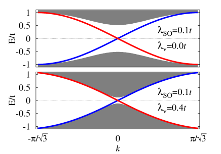
Figure 4: The edge-state energy dispersion of the AC edge for the SOC strength of $\lambda_{SO}=0.1t$. The upper graph shows the energy dispersion without any sublattice potential, and the lower one, with the sublattice potential of $\lambda_{v}=0.4t$. The gray filled regions are the bulk energy spectra. The red and blue solid lines are the edge-state dispersion relations for the spin-up and spin-down electrons, respectively.

Figure 4 shows the edge-state energy dispersion on the AC edge. Without the sub-lattice potential, the edge-state energy dispersion can be expressed as

$$E_{k}^{AC}=t\sin\frac{\sqrt{3}}{2}k,$$ (32)

which is derived in Appendix B. Interestingly, the edge state dispersion is not affected by the SOC on the AC boundary. The SOC modifies only the bulk energy spectrum by changing the bulk energy gap. If we consider the sub-lattice potential, the gap is suppressed due to the competition with the SOC. Increasing the sub-lattice potential makes the gap smaller until the gap is closed at $\lambda_{v}=3\sqrt{3}\lambda_{SO}$, as in the case of the ZZ edge. Unlike the SOC, introducing the sub-lattice potential does not only change the bulk energy spectrum, but also changes the edge-state dispersion. Nevertheless, the modification is quite small and restricted only in the large $k$ region. For small $k$, on the other hand, the edge-state dispersion is still intact despite the parameter change. As seen in Figure 4, the edge-state dispersion with a finite sublattice potential shows only a very small deviation near $k=\pm\frac{\pi}{\sqrt{3}}$.

IV The width of the edge state

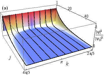
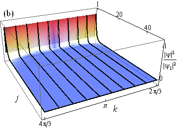
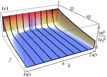
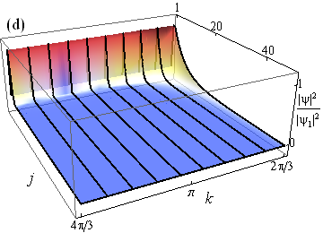
Figure 5: The wave function profile of the edge state of the ZZ edge as a function of the momentum $k$ in $x$-direction (along the edge) and the position $j$ in $y$-direction (perpendicular to the edge). Here, the values of SOC and the sublattice potential are (a) $\lambda_{SO}=0.05t$ and $\lambda_{v}=0$, (b) $\lambda_{SO}=0.15t$ and $\lambda_{v}=0$, (c) $\lambda_{SO}=0.05t$ and $\lambda_{v}=0.2t$, and (d) $\lambda_{SO}=0.15t$ and $\lambda_{v}=0.6t$.

In this section, we investigate spatial behaviors of the edge-state wave function. The edge state appears only when we introduce an edge, and its wave function is expected to be confined at a finite region near the edge. The decaying factor, $\kappa$, in Eq. (9) shows that the wave function decays exponentially as it smears into the inside of the bulk. Figures 5 and 6 show the square of the wave-function amplitude of the spin-up edge state in (15) as a function of the momentum in $x$-direction along the edge and the real space index $j$ in $y$-direction perpendicular to the edge for the ZZ edge and the AC edge, respectively. In both cases, the edge-state wave functions are rather strongly localized near $k=\pi$ for the ZZ edge and $k=0$ for the AC edge. These states gradually evolve to delocalized states as the momentum moves away from the values mentioned above until their energy dispersions submerge to the bulk energy spectra at $k=\frac{2}{3}\pi$ and $\frac{4}{3}\pi$ for the ZZ edge and $k=\pm\frac{\pi}{\sqrt{3}}$ for the AC edge.

For the localization properties of the edge-state wave function, we can define a characteristic length scale from the decaying factor

$$\xi=1/[{\mbox{Re}}~{}\kappa].$$ (33)

This can be denoted as the spatial width of the edge state. The decaying factors are determined by solving the coupled equations (25) and (28) for the ZZ edge, and (13) and (18) for the AC edge. Each edge-state wave function has two decaying factors for the ZZ edge and four decaying factors for the AC edge. Although the physical length scale is actually determined by the smallest decaying factor which gives the longest length scale, we also consider the larger ones since they are useful in analyzing the dependence of the width on the external parameters like the bifurcation behavior as mentioned in our earlier work.Doh and Jeon (2013)

Figure 5 shows the wave function of the edge state near the ZZ edge as a function of the momentum $k$ in $x$-direction and the position $j$ in $y$-direction. The detailed analysis for the ZZ edge was studied in our previous work,Doh and Jeon (2013) where the edge-state width has two length scales on the ZZ edge. The two widths are the same and almost constant near $k=\pi$ as the momentum varies. The widths do not change significantly until the momentum difference from $\pi$ exceeds a certain value which is a function of $\lambda_{SO}$. Right after the momentum exceeds the value, the two widths split into different values. One of them decreases and the other monotonically increases and diverges when the edge-state energy merges into the bulk energy. The splitting of the widths forms a bifurcation behavior.

The spatial wave function profiles of the edge state with the AC edge are shown in Figure 6. The edge state is delocalized when the momentum reaches $k=\frac{\pi}{\sqrt{3}}$ where the energy of the edge state merges into that of the bulk. The largest one of the four edge-state widths monotonically increases as the momentum increases up to $k=\frac{\pi}{\sqrt{3}}$ without any bifurcation behavior or a constant-value region unlike the case of the ZZ edge.

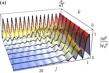
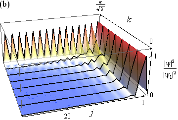
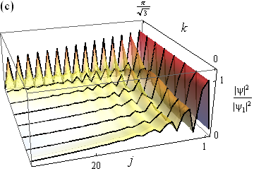
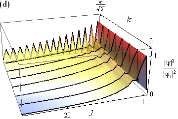
Figure 6: The wave function profile of the edge state with the AC edge as a function of the momentum $k$ in $x$-direction (along the edge) and the position $j$ in $y$-direction (perpendicular to the edge). Here, the values of the SOC and the sublattice potential are (a) $\lambda_{SO}=0.05t$ and $\lambda_{v}=0$, (b) $\lambda_{SO}=0.15t$ and $\lambda_{v}=0$, (c) $\lambda_{SO}=0.05t$ and $\lambda_{v}=0.2t$, and (d) $\lambda_{SO}=0.15t$ and $\lambda_{v}=0.6t$.

The difference between the ZZ edge and the AC edge can be more predominent when we change the strength of SOC. The SOC dependence of the width for the ZZ edge at the momentum $k=\pi$ can be expressed in a simple formCano-Cortés et al. (2013); Doh and Jeon (2013)

$$\xi_{\pi}=a\left[\mbox{arcsinh}\frac{t}{4\lambda_{SO}}\right]^{-1}.$$ (34)

This expression is still valid with the sublattice potential, which only changes the imaginary part of the complex decaying factor.Doh and Jeon (2013) This shows the localized edge state on the ZZ edge actually gets delocalized as the SOC strength increases. On the other hand, increase of the SOC strength enhances localization of the edge state on the AC edge. It is clear when we compare Figures 6 (a) and (b), where the wave function is more squeezed to the edge with the larger SOC strength. According to the numerical results of a nano-ribbon honeycomb lattice, the edge-state width of the AC edge is inversely proportional to the bulk energy gap.Ezawa and Nagaosa (2013) Since the gap is roughly proportional to the SOC strength for the small SOC, the edge-state width of the AC edge decreases as the SOC increases. This is summarized in Figure 7, which shows that the edge-state width of the AC edge monotonically decreases as SOC, $\lambda_{SO}$, increases, while that of the ZZ edge increases.

The broadening of the edge state on the ZZ edge due to the increase of SOC seems counter-intuitive in the sense that SOC develops topologically nontrivial gap in the bulk. Considering the band structure of the Kane-Mele model, however, SOC does not only intensify the topological nature of the system, but also modifies the whole band structure. Without the SOC and the sublattice potential, the honeycomb lattice is semi-metallic with Dirac cones and shows a non-dispersive localized edge state on the ZZ edge like graphene.Fujita et al. (1996); Nakada et al. (1996) In the strong limit of SOC, we can ignore the nearest-neighbor hopping and the sublattice potential term. This makes the system topologically trivial and asymptotically metallic. Therefore, the increase of SOC in the Kane-Mele model does not always intensify the TI state. This explains why the metallic edge state finally delocalizes in the large limit of SOC.

Unlike the SOC, increasing the sublattice potential always drives the system to a topologically trivial insulating state. The transition between the topologically non-trivial to the trivial state should encounter a metallic state due to the topological discontinuity. The edge-state widths also represent this transition. As seen in Figure 7, the edge-state widths on both of the two edges increase as the sublattice potential increases, and finally diverge when the system becomes metallic at $\lambda_{v}=3\sqrt{3}\lambda_{SO}$. Unlike the monotonic increase of the edge-state width of the AC edge, however, that of the ZZ edge shows a transition behavior from a SOC-insensitive state to a SOC-sensitive state as the sublattice potential varies. This originates from the bifurcation of the edge-state width on the ZZ edge. The bifurcation points are denoted as a dotted line in Figure 7.

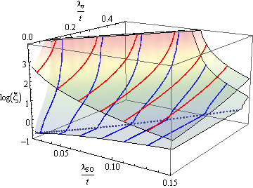
Figure 7: The widths of the edge states at $E=0$ as a function of the SOC and the sub-lattice potential. The upper surface with red lines is for the AC edge, and the lower one with blue lines for the ZZ edge. The blue dotted line denotes the bifurcation points of the widths of the ZZ edge state.

V Edge-state gap for finite system

Although our research is conducted in a semi-infinite lattice, the results is more important in a small system whose size is comparable to the edge-state width. Figure 7 shows that the edge-state width is smaller on the ZZ edge than on the AC edge in nearly entire range of the parameters. If we consider a finite width ribbon of the honeycomb lattice, the metallic edge state of the two dimensional TI system with a finite width is more favorable with the ZZ edge where the edge-state width is small and rather robust to perturbations such as the sublattice potential.

A ribbon with the AC edge can be useful when we try to control the edge-state gap with the sublattice potential. For example, if the honeycomb lattice has a buckled structure having the two sublattices on different planes like silicene, the sublattice potential can be controlled by an external electric field. Since the edge-state width of the AC edge is rather sensitive to the sublattice potential, one can open a band gap at the edge state with a large external electric field.

VI Summary

We derive analytic equations for the edge state of the Kane-Mele model in the semi-infinite honeycomb lattice with a ZZ edge and with an AC edge, respectively. The analytic equations are solved iteratively for the energy and the wave function of the edge state. Our results have no size effects which is inevitable in the numerical calculation of a finite width ribbon. From the analytic form of the wave function of the edge state, we define an edge-state width which is a spatial decaying length of the edge-state wave function perpendicular to the edge. The calculated results of the edge-state width show peculiar behaviors and dependencies on the SOC, the sublattice potential, and the edge types. The localized edge state on the ZZ edge is rather insensitive to the sublattice potential. This gives robust nature of the metallic edge state in a finite sized system. On the other hand, the edge state of the AC edge is easily controllable with the external parameters. Therefore, the edge-state gap of the AC edge can be turned on with the sublattice potential in a finite sized system. Although the edge state of the TI is protected by the topology regardless of the edge type, our results show that the detailed dependence on the edge type can be crucial in small-device manufacturing.

Appendix A Fermi velocity of the edge state on the ZZ edge near $k=\pi$ without sublattice potential.

In this appendix, we derive the Fermi velocity of the edge state on the ZZ edge at $k=\pi$ by expanding the coupled equations (25) and (28) near $k=\pi$. If we ignore the sub-lattice potential $\lambda_{v}$ for the edge state on the ZZ edge, the eigenvalue equation (25) can be simplified as

$$\mathcal{E}^{2}=\left(\cos q-\cosh\kappa\right)^{2}+t^{\prime 2}\left(4\cos^{2}q+4\cos q\cosh\kappa+1\right)$$ (35)

where $q=k/2$,

$$\mathcal{E} \equiv \frac{E}{4\lambda_{SO}\sin q},~{}~{}~{}\mbox{and}$$ (36)

$$t^{\prime} \equiv \frac{t}{4\lambda_{SO}\sin q}.$$ (37)

This is the second order equation of $\cosh\kappa$. The two solutions for $\cosh\kappa$ are

$$\cosh\kappa = \left(1-2t^{\prime 2}\right)\cos q$$ (38)

$$\pm i\sqrt{t^{\prime 2}-4t^{\prime 2}\left(t^{\prime 2}-2\right)\cos^{2}q-\mathcal{E}^{2}},$$

which are complex conjugates of each other. Therefore, the boundary condition (28) can be written as

$${\mbox{Im}}\left[\left(3\cos q-\mathcal{E}\right)\cosh\kappa+\left(\cos q-\mathcal{E}\right)\sinh\kappa\right]$$

$$={\mbox{Im}}\left[\sinh\kappa\cosh\kappa^{\ast}\right]$$

where ${\mbox{Im}}[z]$ is the imaginary part of $z$. Here $\kappa$ is generally a complex number,

$$\kappa=\alpha+i\beta,$$ (39)

where $\alpha$ and $\beta$ are real numbers. From the solution for $\cosh\kappa$, (38), the real numbers, $\alpha$ and $\beta$ satisfy

$$\cosh\alpha\cos\beta = \left(1-2t^{\prime 2}\right)\cos q,$$ (40)

$$\sinh\alpha\sin\beta = t^{\prime}\sqrt{1-4\left(t^{\prime 2}-2\right)\cos^{2}q-\left(\frac{\mathcal{E}}{t^{\prime}}\right)^{2}}.$$ (41)

The boundary condition is rewritten in terms of $\alpha$ and $\beta$ like

$$\left(3\cos q-\mathcal{E}\right)\sinh\alpha+\left(\cos q-\mathcal{E}\right)\cosh\alpha=\cos\beta.$$ (42)

Now we expand $k$ near $\pi$, by replacing $q$ by $\frac{\pi}{2}+\delta q$. If we expand $\delta q$ up to the first order, we get the followings

$$\sinh\alpha \simeq t^{\prime},$$ (43)

$$\cosh\alpha \simeq \sqrt{t^{\prime 2}+1},\mbox{ and}$$ (44)

$$\cos\beta \simeq \frac{2t^{\prime 2}-1}{\sqrt{t^{\prime 2}+1}}\delta q.$$ (45)

After inserting these into (42), we get

$$\mathcal{E} = \frac{(3\sinh\alpha+\cosh\alpha)\cos q-\cos\beta}{\sinh\alpha+\cosh\alpha}$$ (46)

$$\simeq -3\frac{t^{\prime}}{\sqrt{t^{\prime 2}+1}}\delta q.$$

Since $\delta q=\frac{k-\pi}{2}$, the energy dispersion of up-spin near $k=\pi$ on the edge is

$$E\simeq-v_{F}(k-\pi)$$ (47)

where $v_{F}$ is the Fermi velocity at $k=\pi$ with the following form

$$v_{F}=\frac{6\lambda_{SO}t}{\sqrt{t^{2}+16\lambda_{SO}^{2}}}.$$ (48)

Appendix B Energy dispersion of the edge state on AC edge without sublattice potential.

In this appendix, we will find the edge-state energy dispersion on the AC edge by showing that our trial solution for the dispersion satisfies Eq. (13) and (28). Our trial solution for the energy dispersion is $E_{k}=\pm t\sin\frac{\sqrt{3}}{2}k$ which is the envelope function of the bulk energy spectrum for $\lambda_{SO}=0$. If we use this function for the dispersion, the eigenvalue equation (13) is reduced to

$$4\sigma\lambda_{SO}\sinh\kappa\left(\cosh\kappa-\cos q\right)=\pm t\left(\cos q+2\cosh\kappa\right)$$ (49)

where $q=\frac{\sqrt{3}}{2}k$, and $\sigma$ is $\pm 1$ depending on the spin. If we choose the positive sign in front of the nearest-neighbor hopping $t$ in the eigenvalue equation (49), the edge-state wave function for the spin-up electron has negative $\kappa$ and is not confined near the edge. One the other hand, if we choose the negative sign for the dispersion of the spin-up electron as $E_{q}=-t\sin q$, $\kappa$ is positive and the eigenvector is

$$\Phi_{\nu} = \left[\begin{array}[]{c}t\left(1+2e^{iq}\cosh\kappa_{\nu}\right)\\ it\left(\cos q+2\cosh\kappa_{\nu}\right)+t\sin q\end{array}\right]$$ (52)

$$= t\left(e^{-iq}+2\cosh\kappa_{\nu}\right)\left[\begin{array}[]{c}e^{iq}\\ i\end{array}\right].$$ (55)

With this eigenvector, the boundary condition (18) can be reduced to

$$\left|\begin{array}[]{cccc}e^{iq}&e^{iq}&e^{iq}&e^{iq}\\ i&i&i&i\\ e^{-\kappa_{1}}e^{iq}&e^{-\kappa_{2}}e^{iq}&e^{-\kappa_{3}}e^{iq}&e^{-\kappa_{4}}e^{iq}\\ ie^{-\kappa_{1}}&ie^{-\kappa_{2}}&ie^{-\kappa_{3}}&ie^{-\kappa_{4}}\end{array}\right|=0,$$ (56)

which is satisfied trivially because the first and the second rows are linearly dependent. Therefore, the energy dispersion of the edge state of the spin-up electron is, in fact, $E_{q}=-t\sin q$.

References

- Thouless et al. (1982) D. J. Thouless, M. Kohmoto, M. P. Nightingale, and M. den Nijs, Phys. Rev. Lett. 49, 405 (1982).
- Murakami et al. (2003) S. Murakami, N. Nagaosa, and S.-C. Zhang, Science 301, 1348 (2003).
- Kane and Mele (2005a) C. L. Kane and E. J. Mele, Phys. Rev. Lett. 95, 226801 (2005a).
- Kane and Mele (2005b) C. L. Kane and E. J. Mele, Phys. Rev. Lett. 95, 146802 (2005b).
- Bernevig et al. (2006) B. A. Bernevig, T. L. Hughes, and S.-C. Zhang, Science 314, 1757 (2006).
- Bernevig and Zhang (2006) B. A. Bernevig and S.-C. Zhang, Phys. Rev. Lett. 96, 106802 (2006).
- König et al. (2007) M. König, S. Wiedmann, C. Brüne, A. Roth, H. Buhmann, L. W. Molenkamp, X.-L. Qi, and S.-C. Zhang, Science 318, 766 (2007).
- König et al. (2008) M. König, H. Buhmann, L. W. Molenkamp, T. Hughes, C.-X. Liu, X.-L. Qi, and S.-C. Zhang, J. Phys. Soc. Jpn. 77, 031007 (2008).
- Moore and Balents (2007) J. E. Moore and L. Balents, Phys. Rev. B 75, 121306 (2007).
- Fu et al. (2007) L. Fu, C. L. Kane, and E. J. Mele, Phys. Rev. Lett. 98, 106803 (2007).
- Hsieh et al. (2008) D. Hsieh, D. Qian, L. Wray, Y. Xia, Y. S. Hor, R. J. Cava, and M. Z. Hasan, Nature 452, 970 (2008).
- Xia et al. (2009) Y. Xia, D. Qian, D. Hsieh, L. Wray, A. Pal, H. Lin, A. Bansil, D. Grauer, Y. S. Hor, R. J. Cava, and M. Z. Hasan, Nat. Phys. 5, 398 (2009).
- Chen et al. (2009) Y. L. Chen, J. G. Analytis, J.-H. Chu, Z. K. Liu, S.-K. Mo, X. L. Qi, H. J. Zhang, D. H. Lu, X. Dai, Z. Fang, S. C. Zhang, I. R. Fisher, Z. Hussain, and Z.-X. Shen, Science 325, 178 (2009).
- Hsieh et al. (2009) D. Hsieh, Y. Xia, D. Qian, L. Wray, J. H. Dil, F. Meier, J. Osterwalder, L. Patthey, J. G. Checkelsky, N. P. Ong, A. V. Fedorov, H. Lin, A. Bansil, D. Grauer, Y. S. Hor, R. J. Cava, and M. Z. Hasan, Nature 460, 1101 (2009).
- Roushan et al. (2009) P. Roushan, J. Seo, C. V. Parker, Y. S. Hor, D. Hsieh, D. Qian, A. Richardella, M. Z. Hasan, R. J. Cava, and A. Yazdani, Nature 460, 1106 (2009).
- Alpichshev et al. (2010) Z. Alpichshev, J. G. Analytis, J.-H. Chu, I. R. Fisher, Y. L. Chen, Z. X. Shen, A. Fang, and A. Kapitulnik, Phys. Rev. Lett. 104, 016401 (2010).
- Wan et al. (2011) X. Wan, A. M. Turner, A. Vishwanath, and S. Y. Savrasov, Phys. Rev. B 83, 205101 (2011).
- Zhang et al. (2010) Y. Zhang, K. He, C.-Z. Chang, C.-L. Song, L.-L. Wang, X. Chen, J.-F. Jia, Z. Fang, X. Dai, W.-Y. Shan, S.-Q. Shen, Q. Niu, X.-L. Qi, S.-C. Zhang, X.-C. Ma, and Q.-K. Xue, Nat. Phys. 6, 584 (2010).
- Wang et al. (2009) Z. Wang, N. Hao, and P. Zhang, Phys. Rev. B 80, 115420 (2009).
- Harper (1955) P. G. Harper, Proc. Phys. Soc. Lond. A 68, 874 (1955).
- Doh and Jeon (2013) H. Doh and G. S. Jeon, Phys. Rev. B 88, 245115 (2013).
- Ezawa and Nagaosa (2013) M. Ezawa and N. Nagaosa, Phys. Rev. B 88, 121401 (2013).
- Cano-Cortés et al. (2013) L. Cano-Cortés, C. Ortix, and J. van den Brink, Phys. Rev. Lett. 111, 146801 (2013).
- Fujita et al. (1996) M. Fujita, K. Wakabayashi, K. Nakada, and K. Kusakabe, J. Phys. Soc. Jpn. 65, 1920 (1996).
- Nakada et al. (1996) K. Nakada, M. Fujita, G. Dresselhaus, and M. S. Dresselhaus, Phys. Rev. B 54, 17954 (1996).