The estimation of neutrino flux produced by $\mathbf{pep}$ reactions in the Sun

Abstract

The experimental result of the solar neutrino flux at one AU produced by the $p+p+e\rightarrow d+\nu_{e}$ reaction (pep) was announced for the first time in 2012 by the Borexino collaboration. This neutrino flux was significantly greater than the flux predicted by Bahcall and May, who used two body approaches for calculation of this reaction. We have used the three-body model for the proton-proton-electron system in the continuous spectrum of energy to determine the rate of the pep reaction and have estimated the neutrino flux. Our result of the neutrino flux is 25-40% more than the Bachall et al. value and depends on the shape of nucleon-nucleon ($NN$) potential. Moreover, the calculated flux lies within the confidence interval of the experimental data in the case of pure attractive potentials as well as potential having repulsion at small distances between nucleons.

(Some figures may appear in color only in the online journal)

1 Introduction

The measurement of the neutrino flux from the Sun gives possibility to solve several important problems. A careful study of the solar neutrino flux penetrating the Earth gives possibility to understand many characteristics of the neutrino including the effect of the neutrino oscillation, estimation of mixing angle and neutrino mass. The neutrino flux along with its spectral properties give us useful insight to nuclear reactions which otherwise cannot be observed under terrestrial conditions. The main reaction called $pp$ reaction going in the interior of the Sun and determining the luminosity is

$$p+p\rightarrow d+e^{+}+\nu_{e}.$$ (1)

Furthermore, as underlined by John N. Bahcall in his series of papers and book [1, 2, 3, 4, 5, 6], solar neutrinos bring the signals from processes in the core of star,and allow one to make comparison of the data with solar structure models. Unfortunately it is impossible to directly measure the neutrino flux from this reaction in the laboratory. The reaction

$$p+p+e^{-}\rightarrow d+\nu_{e},$$ (2)

which is called $pep$ reaction stimulates interest because an emitted neutrino is monoenergetic even though $pep$ plays no essential role in hydrogen burning in the Sun. The energy of neutrino from this reaction is $E_{\nu}=1.44$ MeV. The parameters of the Standard Solar Model can be estimated from measurement of the neutrino flux coming from the pep reaction.

Bahcall and May [7] used the two-body approach for considering the three-body $pep$ reaction [8]. In the abstract of Ref. [9] the authors presented some qualitative estimation of the three-body effect for $pep$ reaction and came to the conclusion that the previous conventional estimation of the $pep$ solar neutrino flux could have been underestimated. Therefore the solution of the three-body equation without applying two-body approximation was required.

The purpose of this work is to treat the the initial state of the reaction (2) as a purely three-body state. It is well known fact that low energy nucleon-nucleon data is insensitive to the form of $NN$ potential in the two body case. However, the three-body system is sensitive to the type of the potential. The idea behind this work is to check the sensitivity of neutrino flux to a used $NN$ potential, within different Standard Solar Models, and most important to extend our previous results [10] by using a realistic $NN$ potential. It took more than fifty years, after the existence of solar neutrino problem, for the announcement of the first experimental observation of process (2) [11]. Further a three-body description of the initial state in process (2) with different types of $NN$ potential was not available in literature. These were the main motivation for presenting our current calculation.

In Sec. 2 we briefly introduce our weak Hamiltonian and the two types of nucleon-nucleon potentials. We determine the probability and the astrophysical $S_{pep}$ factor of the reaction (2) in Section 3. The reaction rate and calculation of solar neutrino flux is presented in Section 4. We finally conclude and summarize our calculation in Section 5.

In this paper, we applied the same notation for the quantities as in our previous article [10].

2 Inputs

Electron capture by the nuclei with emitting electron neutrino is considered by the application of the effective Hamiltonian (nonrelativistic) describing weak interaction presented in Ref. [12]. Taking into account the smallness of the neutrino energy in the reaction $pep\rightarrow d+\nu_{e}$ as well as the ansatz that the transition satisfies the Gamow-Teller selection rule we reduce the weak transition operator to the form:

$$H_{w}=\tau^{(+)}G_{A}\sum\limits_{i=1}^{2}\tau_{i}^{(-)}\mathbf{\sigma\cdot\sigma_{i}}\delta{\mathbf{(r-r_{i})}},$$ (3)

where $\mathbf{\sigma}$ and $\mathbf{\sigma_{i}}$ are spin operators for the lepton and ith nucleon; $\mathbf{r}$ and $\mathbf{r_{i}}$ are the space coordinates of the lepton and an ith nucleon; $\tau^{(+)},\,\,\tau^{(-)}_{i}$ are the isobaric-spin operators transforming a lepton electron state into a lepton neutrino state and ith nucleon proton state into an ith nucleon neutron state, respectively. We used axial vector coupling constant $G_{A}$ equaling to $G_{A}/(\hbar c)^{3}=-1.454\times 10^{-11}\,\rm{GeV}^{-2}$ [13].

In our previous calculation [10] we used the simplest potentials (Gauss and Yukawa types) which are pure attractive in nature. In this work we apply one more simplest exponential potential and in addition a realistic $NN$ potential (Malfliet-Tjon potential [14]) having repulsion at small distance to check sensitivity of the flux from the reaction (2) to the shape of potential.

The fitted parameters to these potentials listed below determine correctly the low energy $NN$ scattering data and binding energy of the deuteron.

The parameters of the exponential potential

$$V^{N}(r)=-V_{0}\exp\bigl{(}-r/R_{N}\bigr{)}$$ (4)

describing the low energy $NN$ data at the singlet ($s$) and triplet ($t$) states are

$$V_{0}^{s}={\rm 98.10\;MeV,\;}\,\,\,\,R_{N}^{s}={\rm 0.744\;fm};$$

$$V_{0}^{t}={\rm 184.08\;MeV,\;\;}R_{N}^{t}={\rm 0.683fm}.$$

These parameters define the following scattering lengths and effective ranges

$${}^{s}a_{pp} = -7.874\,\,{\rm{fm}},\,\,\,\,^{s}r_{pp}=2.804\,\,{\rm{fm}},$$

$${}^{t}a_{np} = \,\,\,\,\,5.403\,\,{\rm{fm}},\,\,\,\,^{t}r_{np}=1.716\,\,{\rm{fm}}.$$ (5)

The M-T potential is

$$V^{N}(r)=\frac{V_{A}}{r/R_{A}}\exp\bigl{(}-r/R_{A}\bigr{)}+\frac{V_{R}}{r/R_{R}}\exp\bigl{(}-r/R_{R}\bigr{)}.$$ (6)

Fitting of $NN$ low energy data gives the following parameters of the M-T potentials:

$$V_{A}=-{\rm 898.75\;MeV,\;}R_{A}={\rm 0.617\;fm},$$

$$V_{R}={\rm 4319.85\;MeV,\;\;}R_{R}={\rm 0.325\,fm},$$

for the singlet state and

$$V_{A}={-\rm 945.50\;MeV,\;}R_{A}^{t}={\rm 0.645\;fm},$$

$$V_{R}={\rm 4476.845\;MeV,\;\;}R_{R}^{t}={\rm 0.322\;fm},$$

for the triplet state. Here we omitted indexes $s$ and $t$ to simplify entries. These parameters determine the scattering lengths and effective ranges:

$${}^{s}a_{pp} = -7.88\,\,{\rm{fm}},\,\,\,\,^{s}r_{pp}=2.69\,\,{\rm{fm}},$$

$${}^{t}a_{np} = \,\,\,\,\,5.52\,\,{\rm{fm}},\,\,\,\,^{t}r_{np}=1.89\,\,{\rm{fm}}.$$ (7)

The indexes $s$ and $t$ mean the singlet and triplet state, respectively.

To find the neutrino flux some Standard Solar Model (SSM) must be used. The results of Bahcall et al. [4] showed that the sensitivity of the flux of neutrino from the $pp$ and $pep$ reactions to the type of SSM was very weak. In previous calculation we used the parameters of the BS2005(OP) model presented on website [15]. For the case of the exponential potential we use additionally BP2000 Solar Standard Model [15] to check sensitivity of the flux to the type of SSM.

3 The probability of the $\mathbf{pep\to d+\nu}$ reaction

It should be noted that Bahcall and May [7] used the adiabatic approximation for the wave function of the $pep$ system. In this approach the $pep$ wave function was presented by the product of the wave function of electron moving relative to the center of mass of the two protons and the wave function of the relative motion of two protons. Unfortunately, such a description is not adequate even in the region where the distance from the center of mass of the protons to electron far exceeds the size of nucleon-nucleon system due to the nature of the Coulombic force [16]. Moreover, we cannot use the such factorized wave function at the region of the small distances between the particles where it is necessary to know the wave function with a sufficient accuracy to perform a precise calculation of the transition matrix element of the process $pep\to d\nu_{e}$.

In our paper [10] we showed the use of hyperspherical harmonics method [17, 18] to directly solve the 3-body Schrödinger equation for $pep$ system. Deduction of one-dimensional coupled radial equations can be found in our article [10]. Due to the smallness energy of the colliding particles we restrict ourselves by consideration of the radial equation assuming that all quantum numbers are zero. Therefore we solve the following radial equation:

$$\frac{d^{2}U(\rho)}{d\rho^{2}}+\frac{1}{\rho}\frac{dU}{d\rho}-\Bigl{(}{\cal{V}}(\rho)+\frac{4}{\rho^{2}}-\kappa^{2}\Bigr{)}U(\rho)=0,$$ (8)

where $\kappa^{2}=2\mu_{23}E/\hbar^{2}>0$ ($E$ is the total energy of the colliding particles in the $pep$ system);

$${\cal{V}}(\rho)\,\,\,\, = {\cal{V}}^{N}(\rho)+{\cal{V}}^{C}(\rho),$$ (9)

$${\cal{V}}^{C}(\rho) = \frac{32\mu_{23}}{3\pi\hbar^{2}}\frac{(a_{1}+a_{2}+a_{3})}{\rho}\equiv\frac{2\eta_{3}\kappa}{\rho}.$$ (10)

Here $\eta_{3}$ is the 3-body Coulomb parameter (analogue of the Sommerfeld parameter) which is defined as

$$\eta_{3} = \frac{16\mu_{23}}{3\pi\hbar^{2}\kappa}(a_{1}+a_{2}+a_{3}),$$ (11)

$$a_{1} = \sqrt{\frac{m_{2}m_{3}}{\mu_{23}(m_{2}+m_{3})}}e^{2}\equiv e^{2},$$ (12)

$$a_{2} = -\sqrt{\frac{m_{1}m_{3}}{\mu_{23}(m_{1}+m_{3})}}e^{2}\simeq-\sqrt{\frac{2m_{1}}{m_{3}}}e^{2},$$ (13)

$$a_{3} = -\sqrt{\frac{m_{1}m_{2}}{\mu_{23}(m_{1}+m_{2})}}e^{2}\simeq-\sqrt{\frac{2m_{1}}{m_{2}}}e^{2}.$$ (14)

${\cal{V}}^{N}$ and ${\cal{V}}^{C}(\rho)$ are the reduced nuclear and Columbic potentials resulting due to integration by applying the hyperspherical function of zero value of the hypermoment. These potential can be easier calculated analytically for the considered potentials.

To find numerically a solution of Eq. (8) we use the following boundary condition at the point $\rho_{0}$ closed to the origin:

$$U(\rho_{0})=J_{2}(\kappa_{0}\rho_{0}),\,\,\,\,U^{\prime}(\rho_{0})=\kappa_{0}J_{2}^{\prime}(\kappa_{0}\rho_{0}),$$ (15)

in the case ${\cal{V}}^{N}(\rho_{0})<0$ (pure attractive potential) or

$$U(\rho_{0})=I_{2}(\kappa_{0}\rho_{0}),\,\,\,\,U^{\prime}(\rho_{0})=\kappa_{0}I_{2}^{\prime}(\kappa_{0}\rho_{0}),$$ (16)

in the case ${\cal{V}}^{N}(\rho_{0})>0$ ($NN$ potential is repulsive near the origin). Here $\kappa_{0}=\sqrt{\kappa^{2}+\mid{\cal{V}}^{N}(\rho_{0})\mid}$ $(\kappa_{0}=\sqrt{{\cal{V}}^{N}(\rho_{0})-\kappa^{2}}$ if ${\cal{V}}^{N}(\rho_{0})>0$), $J_{2}(x)$ is the Bessel function and $I_{2}(x)$ is the modified Bessel function. Such boundary condition follows from behavior of the radial function near origin. It is clear to see that $U(\rho)\sim\rho^{2}$ if $\rho\to 0$ for any type of $NN$ potential without hard core.

The asymptotic of the radial function $U(\rho)$ at large distance ($\rho\rightarrow\infty$) is:

$$U(\rho)\longrightarrow e^{i\delta_{3}}\cos\delta_{3}\bigl{(}F_{00}(\kappa\rho)-\tan\delta_{3}G_{00}(\kappa\rho)\bigr{)},$$ (17)

where $\delta_{3}$ is the 3-body nuclear scattering phase shift modified by the Coulomb interactions. At the considered low energy range the phase $\delta_{3}\sim 0$ and according to Ref. [17] the 3-body Coulombic phase shift is given by

$$\delta_{3C}=\arg\left[\Gamma(5/2+i\eta_{3})\right],$$ (18)

and $F_{00}(\kappa\rho)$ and $G_{00}(\kappa\rho)$ are the 3-body regular and irregular Coulomb wave functions [17]. A reader can find the representations of these functions in our paper [10].

Eq. (8) was solved using the boundary conditions (15) or (16) depending on the behavior of the $NN$ potential near origin. Equating the logarithmic derivative of the numerical solution at distance where the nuclear potential is negligible to the logarithmic derivative of the asymptotic solution [Eq. (17)] we find the 3-body phase shift $\delta_{3}$. The result for $U(\rho)$ obtained with the Gauss potential was shown in Figure 1 of Ref. [10]. We got the same results with the Yukawa and exponential potentials. The limit of $U(\rho)/(\kappa\rho)^{2}$ goes to nonzero value. However, near the origin, the behavior of the curve describing solution with the M-T potential differs from the solution applying simple potentials. In this case the limit of $U(\kappa\rho)/(\kappa\rho)^{2}$ approaches to the value close to zero due to the repulsive term in the M-T potential which becomes very large at small distance. However, the behavior of radial function is almost the same at large distance like for the simplest potentials having only attraction term. At sufficiently large distances, the ratio of the unnormalized solution of the equation of Eq.(8) to the asymptotic function given by Eq. (17) becomes constant for all considered cases. It allowed us to get the normalized wave function [10]. The matching distance depends on the type of potential and lies at a distance $\sim$35 fm for the case of the simple $NN$ potentials and in the case of M-T potential matching distance is $\sim$50 fm owing to its repulsive part of interaction. It should be noted that the wave function of $pp$ system can be replaced by its asymptotics already from a distance of $\sim$5 fm. For this reason, the rate of the $pp$ reaction is insensitive to the choice of potential. At the same time in the calculation of the $pep$ reaction the wave function of $pep$ system can be replaced by its asymptotics from a distance of only $\sim$35-50 fm, but for the distance less than 35 fm we must use the exact 3-body wave function. The 3-body wave function must be calculated with sufficient accuracy at range $0<\rho<35$ fm because the deuteron wave function decays exponentially to zero around 35 fm. Interested readers can study dependence of the $pep$ 3-body wave function on the hyperradius in Figure 1 of our paper [10].

Applying the weak Hamiltonian (Eq. (3)) the matrix element for the $pep\to d\nu$ transition can be written as

$$H_{if} = G_{A}<\varphi_{\nu}\mid{\mathbf{\sigma}}\tau^{(+)}\mid\varphi_{e}>\times$$ (19)

$$\sum\limits_{i=1}^{2}<\Psi_{d}\Psi_{\nu}\mid{\mathbf{\sigma}}_{i}\tau_{i}^{(-)}\mid\Psi_{pep}>,$$

where $\varphi_{\nu}$ and $\varphi_{e}$ refer the spin functions of neutrino and electron, respectively; the wave function of the deuteron is denoted by $\Psi_{d}$, and $\Psi_{pep}$ is the $pep$ wave function. We take the neutrino wave function $\Psi_{\nu}$ as a plane wave which can be replaced by unity owing to cutoff of the integration interval in the calculation of the matrix element (Eq. (19)). Due to the zero-range weak interaction of electron with proton the electron coordinate in the wave function $\Psi_{pep}$ is taken at the point where either of the protons is located.

The probability $P_{3}$ of reaction per unit time was calculated using the first-order perturbation theory in the weak interaction. We define the probability $P_{3}$ as

$$P_{3}=\frac{2\pi}{\hbar}\overline{\mid H_{w}\mid^{2}}\rho(E_{\nu}),$$ (20)

where the density of neutrino states is

$$\rho(E_{\nu})=\frac{E_{\nu}^{2}}{2\pi^{2}\hbar^{3}c^{3}}.$$ (21)

Here $E_{\nu}=$1.44 MeV is the neutrino energy and $c$ is light speed.

Finally, we get the equation for the probability $P_{3}$ of the $pep\to d\nu$ reaction in form:

$$P_{3}=\frac{3E_{\nu}^{2}G_{A}^{2}}{\pi\hbar^{4}c^{3}}\mid\int\Psi^{*}_{d}({\mathbf{x}})\Psi_{pep}({\mathbf{x,y_{0}}})d^{3}x\mid^{2},$$ (22)

where ${\mathbf{y_{0}}}$ is a Jacobi coordinate of the electron at the point where it contacts with one of the protons.

The overlap integral of Eq. (22) can be reduced to the one dimensional integral:

$$\int\Psi_{d}^{*}({\mathbf{x}})\Psi_{pep}({\mathbf{x,y_{0}}})d^{3}x=\frac{16\sqrt{\pi}}{\kappa^{2}}\int\limits_{0}^{\infty}x^{-1}\chi_{d}(x)U(x)dx.$$ (23)

Here the function $U(\rho)$ is taken at the point $\rho=\sqrt{x^{2}+y_{0}^{2}}\simeq x$ ($x\gg y_{0}$) and the radial wave function $\chi_{d}(x)$ of the deuteron is normalized to unity. Figure 1 shows the results of the dependence of the integrand of the matrix element (23) calculated with the exponential and M-T potentials. We see that the integrands depend on whether the $NN$ potential has repulsion at small distances or whether it is a purely attractive potential.

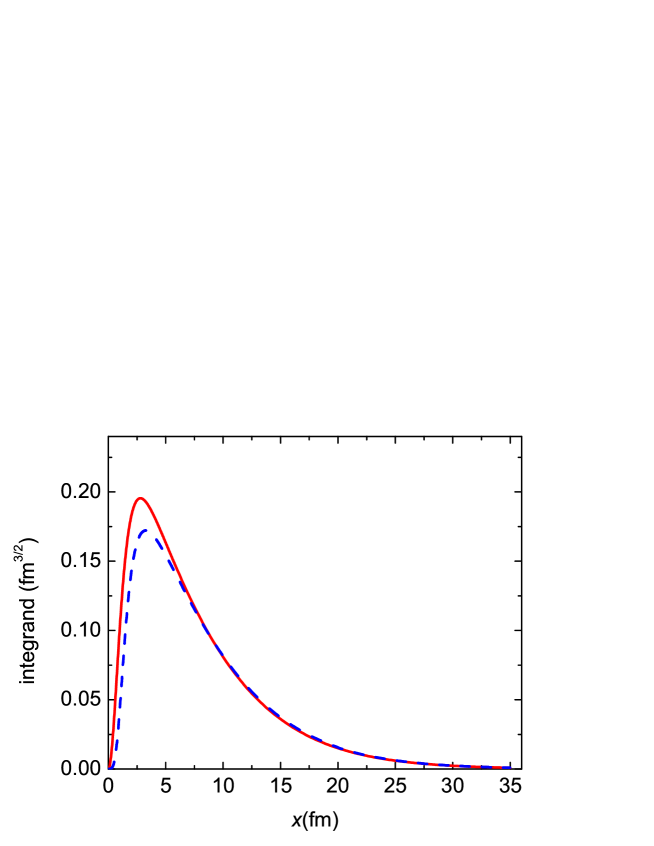
Figure 1: The dependence of the integrand in Eq. (23) on the distance calculated with the exponential (solid line) and M-T potentials (dashed line) at $E_{pep}$=8 keV.

In nuclear astrophysics the rate of the binary reaction is calculated using the astrophysical $S$ factor [19]. The cross section of such reactions is related to the astrophysical $S$ factor as

$$\sigma(E)=\frac{S(E)}{E}e^{-2\pi\eta},$$ (24)

where $\eta=Z_{1}Z_{2}e^{2}/(\hbar v)$ is the Sommerfeld parameter, $Z_{1}e$ and $Z_{2}e$ are charges of colliding nucleus with the relative velocity $v$. The factor $\exp(-2\pi\eta)$ is proportional to the probability of the penetration of a charged particle through the Coulomb barrier. In the $pep$ reaction we can adopt a similar parameter because the 3-body $pep$ radial wave function $U(\rho)$ encloses the factor $\exp(-\pi\eta_{3}/2)\mid\Gamma(5/2+i\eta_{3})\mid$ owing to the Coulomb interaction between colliding particles. Therefore we can identify the Coulombic factor in the probability $P_{3}$ and define the astrophysical $S_{pep}$ factor for the $pep$ reaction as

$$P_{3}(E) = G_{0}(E)S_{pep}(E),$$ (25)

$$G_{0}(E) = \frac{2\pi e^{-2\pi\eta_{3}}(\frac{1}{4}+\eta_{3}^{2})(\frac{9}{4}+\eta_{3}^{2})}{1+e^{-2\pi\eta_{3}}}.$$ (26)

For range of energy close to zero, our results show that $S_{pep}(E)$ varies almost linearly with energy $E$. Its limit is not zero when the energy goes to zero. Also we note that $G_{0}(E)$ is dimensionless therefore the $S_{pep}(E)$ dimension coincides with the unit of $P_{3}(E)$ according to our definition of this quantity. Due to linear property of $S_{pep}(E)$ at low energies we can expand it into a series and restrict ourselves to first three terms, so we write

$$S_{pep}(E)=S_{0}+S_{1}E+S_{2}E^{2},$$ (27)

The calculated results for the value of the coefficients are following:
the exponential potentials

$$S_{0} = 2.49\times 10^{10}\rm{fm^{6}/s},$$

$$S_{1} = 3.35\times 10^{10}\rm{fm^{6}/(MeV\,s)},$$

$$S_{2} = 2.21\times 10^{10}\rm{fm^{6}/(MeV^{2}\,s)};$$ (28)

and the M-T potentials

$$S_{0} = 2.11\times 10^{10}\rm{fm^{6}/s},$$

$$S_{1} = 3.70\times 10^{10}\rm{fm^{6}/(MeV\,s)},$$

$$S_{2} = 1.76\times 10^{10}\rm{fm^{6}/(MeV^{2}\,s)}.$$ (29)

The coefficients $S_{0}$, $S_{1}$ and $S_{2}$ for the Gauss and the Yukawa potential are given in Ref. [10]. We note the difference between values of the coefficients $S_{0}$ for considered simple potentials (Gauss, Yukawa, exponential) can reach $\sim$3-6%, while the difference for the coefficient $S_{0}$ calculated with M-T potentials reaches $\sim$15% with respect to the simplest potentials. The difference for the coefficients $S_{1}$ and $S_{2}$ goes to much larger values. Fortunately the contribution of $S_{1}$ and $S_{2}$ to the flux of neutrino is much less as compared to $S_{0}$. We would also like to mention that the analogue astrophysical $S$ factor for two particle reaction (1) does not depend on the type of $NN$ potential in contrast to the three particle astrophysical $S$ factor defined by Eq. (26).

4 Rate and flux of the solar neutrinos

We define the rate constant of the $pep$ reaction [10] by following equation

$${\cal{K}}_{pep}=<P_{3}>=\int\limits_{0}^{\infty}\int\limits_{0}^{\infty}\int\limits_{0}^{\infty}\varphi(v_{e})\varphi(v_{p_{1}})\varphi(v_{p_{2}})P_{3}(E)dv_{e}dv_{p_{1}}dv_{p_{2}}.$$ (30)

After averaging over the Maxwell-Boltzmann distributions $\varphi(v_{i})$ describing the random motion of protons and electrons in the core plasma of the Sun we get the simple formula for the rate constant expressed though the 3-body astrophysical $S_{pep}$ factor:

$${\cal{K}}_{pep}=\frac{1}{(kT)^{3}}\int\limits_{0}^{\infty}G_{0}(E)S_{pep}(E)e^{-E/kT}E^{2}dE,$$ (31)

where $k$ is the Boltzmann constant and $T$ is temperature in the core of the Sun. The maximum of the integrand is reached at the energy

$$E_{max}=\Bigl{(}\frac{1}{2}kT\sqrt{E_{G}}\Bigr{)}^{2/3}.$$ (32)

Here $E_{G}$ is the Gamow energy for $pep$ reaction [10].

The rate of reaction related to the rate constant is

$${\cal{R}}_{pep}={\cal{K}}_{pep}n_{p}^{2}n_{e},$$ (33)

where $n_{e}$ and $n_{p}$ are the density of the reactants (protons and electrons).

In our calculation of the $pp$ and $pep$ reaction rates we applied the BS2005(OP) SSM [6] for both type of $NN$ potentials. The $pp$ and $pep$ reaction rates do not depend much on the type of the solar model (for details we refer to [5]). Additionally we used BP2000 SSM for calculation of the rate with the exponential potentials to check sensitivity of the results to the SSMs.

In Figure 2 we present the dependence of the rate of the $pep$ and $pp$ reactions on the solar interior calculated by the exponential and M-T potentials. The rate of $pp$ reaction differs within 2.4% for all type of used potentials, including the potential used in Ref. [10]. Therefore in the figure the rate of $pp$ reaction is shown only for the exponential potential. There is a small difference of the rate of $pep$ reaction calculated by applying the simplest attractive potentials. However, in the case of M-T potential it differs within $\sim$10-15% from the rates calculated with the simplest potentials.

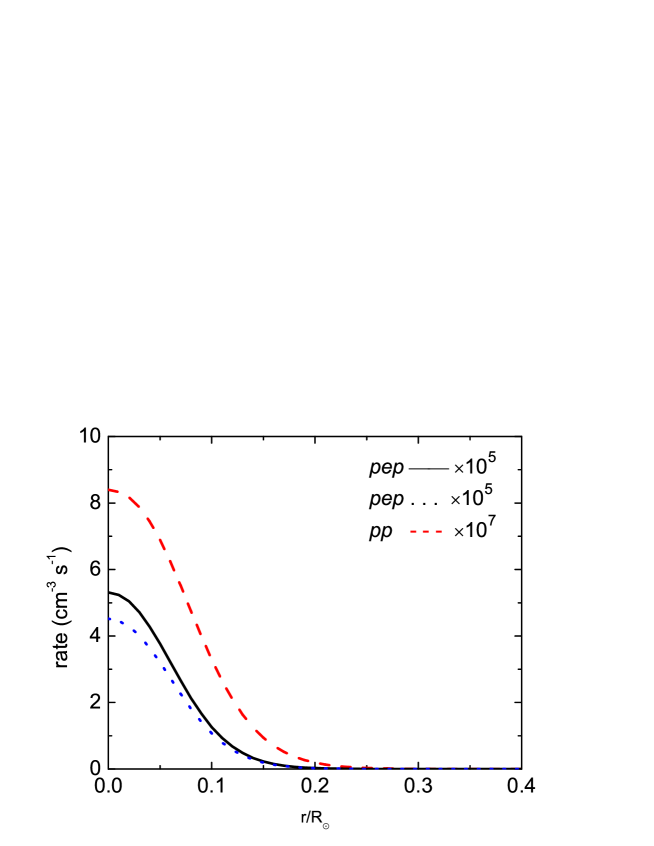
Figure 2: The $pep$ (solid line for exponential potential and dotted line for M-T potential) and $pp$ (dashed line for exponential potential) rates vs. the solar interior. The results of the $pp$ rate is almost same for the exponential and M-T potentials. BS2005 (OP) SSM is applied.

Finally we present, in Table 1, the results of calculation of the fluxes of neutrinos at a distance of one astronomical unit (AU).

Table 1: Predicted fluxes $\Phi_{pp}$ and $\Phi_{pep}$ (without survival probability), in units of $10^{10}\,(pp),10^{8}\,(pep)\,\,\rm{cm^{-2}s^{-1}}$.

Standard Solar	$\Phi_{pp}$	$\Phi_{pep}$	$\Phi_{pp}/\Phi_{pep}$	References
Model
BS2005(OP)	6.20	2.04	304	using Gauss potential [10]
	6.05	1.99	304	using Yukawa potential [10]
	6.13	2.14	287	using exponential potential
				(current work)
	6.16	1.82	338	using M-T potential (current work)
BP2000	6.02	2.10	288	using exponential potential
				(current work)
BP04(Yale)	5.94	1.40	424	[4]
BP04(Garching)	5.94	1.41	421	[4]
BS04	5.94	1.40	424	[4]
BS05(14N)	5.99	1.42	421	[4]
BS05(OP)	5.99	1.42	421	[4]
BS05(AGS,OP)	6.06	1.45	418	[4]
BS05(AGS,OPAL)	6.05	1.45	417	[4]

One notes that whereas our results of calculated flux of neutrino for $pp$ reaction are close to the Bahcall et al. results but differences exist for the calculated results of the $pep$ reactions.

If we take into account the Borexino collaboration measured neutrino flux ($\Phi_{pep}=(1.6\pm 0.3)\times 10^{8}\,{\rm{cm}}^{-2}{\rm{s}}^{-1}$) and the survival probability of the electron neutrino ($P=0.62\pm 0.17$ at 1.44 MeV) suggested by this group [11] we find that the neutrino flux at 1 AU should be equal to $\Phi_{pep}=(1.33\pm 0.36)\times 10^{8}\,\,{\rm{cm}}^{-2}{\rm{s}}^{-1}$ for the exponential potential, and $\Phi_{pep}=(1.13\pm 0.31)\times 10^{8}\,\,{\rm{cm}}^{-2}{\rm{s}}^{-1}$ for the M-T potential if the BS2005(OP) Standard Solar Model is used. Applying BP2000 Standard Solar model leads to the flux equal to $\Phi_{pep}=(1.30\pm 0.36)\times 10^{8}\,\,{\rm{cm}}^{-2}{\rm{s}}^{-1}$ in the case of the exponential potential.

We see that our calculated neutrino fluxes from the $pep$ reaction lie within the confidence interval of the experimental data for all considered simplest potentials including the exponential potential even if we multiply the calculated fluxes by the survival probability ($P=0.62\pm 0.17$) suggested by Borexio group. The flux calculated by using M-T potential lies at the lower limit of the confidence interval. If we multiply the fluxes of neutrino from $pep$ reaction calculated by Bahcall et al. to the value of survival probability all their results lie out of the confidence interval of the Borexino data.

Averaging the Bahcall et al. fluxes from $pp$ reaction presented in Table 1 give us the value equal to $\Phi_{pp}=5.99\times 10^{10}\,{\rm{cm}}^{-2}{\rm{s}}^{-1}$ and with standard deviation equal to $0.05\times 10^{10}\,{\rm{cm}}^{-2}{\rm{s}}^{-1}$. Comparing the fitted low-energy parameters for the simplest potentials, we see that the difference between effective range parameters may be 2%-7%, at the same time the neutrino fluxes from the $pp$ reaction have a 3.5% maximal difference from the average value of Bahcall result (in the case of the Gauss potential, BS2005 (OP) SSM). This means the fluxes from $pp$ reaction is insensitive to the type of $NN$ potential and to SSM. However, the difference between the fluxes of neutrinos from $pep$ reaction calculated by the simplest potentials and the potential having repulsion at small distances (M-T potential) may reach $\sim 15\%$. Consequently our results from $pep$ reaction is expected to show dependence on the type of used $NN$ potential. Also we must note that the difference between our results and Bahcall et al. results for $pep$ process can reach up to 25% to 40%, and indicates strong dependence on the selection of the initial 3-body state of the $pep$ system.

5 Conclusion

The process $pep\to d+\nu_{e}$ has been considered for the first time within the framework of the 3-body description of the initial state employing the nucleon-nucleon potential having repulsion at small distances. The rate and the flux of neutrino from $pp$ and $pep$ reactions has been calculated for specific conditions in the center of the Sun. The theoretical results are in satisfactory agreement with the reported measured data by the Borexino group, but different by (25-40)% from previous calculations made by Bahcall et al. For a better comparison between theory and measurement it is necessary to reduce uncertainty in oscillation parameters of oscillation of neutrinos and to make a new calculation using other realistic nucleon-nucleon potentials having repulsive core.

References

References

- [1] J. N. Bahcall, Neutrino Astrophysics, (Cambridge University Press, Cambridge) 1989.
- [2] J. N. Bahcall, Nucl. Phys. Proc. Suppl. 118, 77 (2003).
- [3] J. N. Bahcall, and M. H. Pinsonneault, Phys. Rev. Lett. 92, 121301 (2004).
- [4] J. N. Bahcall, A. M. Serenelli, and S. Basu, ApJ 621, L85 (2005); arXiv:astro-ph/0412440.
- [5] J. N. Bahcall, A. M. Serenelli, and S. Basu, ApJ Suppl. 165, 400 (2006).
- [6] http://www.sns.ias.edu/jnb/
- [7] J. N. Bahcall and R. M. May, ApJ 155, 501 (1969).
- [8] V. B. Belyaev, S. V. Levin, S. L. Yakovlev, J. Phys. B37, 1369 (2004).
- [9] Y. E. Kim, A. L. Zubarev, http://adsabs.harvard.edu/abs/1996APS..MAY.C1003K.
- [10] B. F. Irgaziev, V. B. Belyaev,and Jameel-Un Nabi, Phys. Rev. C, 035804 (2013).
- [11] G. Bellini et al. (Borexino Collaboration), Phys. Rev. Lett. 108, 051302 (2012).
- [12] H. Primakoff, Rev. Mod. Phys. 31, 802 (1959).
- [13] B. Povh, K. Rith, C. Scholz, F. Zetsche, Particles and Nuclei: An Introduction to the Physical Concepts, 6th ed. (Springer-Verlag, Berlin, Heidelberg, 2008).
- [14] R. A. Malfliet, J. A. Tjon, Nucl. Phys. A127, 161 (1969).
- [15] http://www.sns.ias.edu/jnb/SNdata/Export/BS2005/ bs05op.dat.
- [16] E. O. Alt and A. M. Mukhamedzhanov, Phys. Rev. A 47, 2004 (1993).
- [17] R. I. Djibuti and K. V. Shitikova, Metod hipersfericheskih funktsiy v atomnoy i yadernoy fizike (Method of hyperspherical functions in atomic and nuclear physics), (Energoatomizdat,Moscow, 1993),in Russian.
- [18] M.Fabre de la Ripelle, The hyperspherical expansion method, in: Models and Methods in Few-Body Physics (Lect. Notes Phys., Vol. 273) (L. S. Ferreira, A. C. Fonseca, and L. Streit, eds.), Springer, Berlin (1987), p. 283.
- [19] C. Angulo et al., Nucl. Phys. A 656, 3 (1999).