Integral manifolds of the reduced system
in the problem of inertial motion
of a rigid body about a fixed point

Let $A$, $B$ and $C$ $(A<B<C)$ be the principal moments of inertia of a rigid body having a fixed point. We consider the ellipsoid ${E}^{2}$ defined in $\mathbb{R}^{3}$ by the equation $Ax^{2}+By^{2}+Cz^{2}=1$ with the following metric on its surface

$$d\Sigma=\sqrt{hABC}\left(A^{2}x^{2}+B^{2}y^{2}+C^{2}z^{2}\right)^{-\frac{1}{2}}d\sigma.$$

Here $h>0$ is a constant, $d\sigma$ is the metric on ${E}^{2}$ induced by the scalar product of $\mathbb{R}^{3}$. The reduced system [1] of the problem of the motion of a rigid body with a fixed point without external forces is equivalent to the Hamiltonian system on $T^{*}{E}^{2}$ with the Hamilton function

$${H=\frac{A^{2}x^{2}+B^{2}y^{2}+C^{2}z^{2}}{2ABC}(p_{x}^{2}+p_{y}^{2}+p_{z}^{2})}.$$ (1)

The projections to ${E}^{2}$ of the integral curves of this system with constant energy $H=h$ are, according to the Maupertuis principle, geodesics of the metric $d\Sigma$. Thus, instead of saying ‘‘the basic integral curve of the Hamiltonian vector field $X_{H}$’’ we use the term ‘‘geodesic’’.

Proposition 1.

Any integral manifold $J_{h}=\{H=h\}$ in $T^{*}{E}^{2}$ is diffeomorphic to $T_{1}^{*}S^{2}$, i.e., to the bundle of the unit cotangent vectors to the sphere.

Proof.

Let $D$ be the diffeomorphism of ${E}^{2}$ onto $S^{2}=\{\xi^{2}+\eta^{2}+\zeta^{2}=1\}$ such that $D(x,y,z)=(\sqrt{A}x,\sqrt{B}y,\sqrt{C}z)$. The corresponding diffeomorphism of the cotangent bundles $T^{*}D:T^{*}S^{2}\to T^{*}{E}^{2}$ has the form $x=\xi/\sqrt{A}$, $y=\eta/\sqrt{B}$, $z=\zeta/\sqrt{C}$, $p_{x}=\sqrt{A}p_{\xi}$, $p_{y}=\sqrt{B}p_{\eta}$, $p_{z}=\sqrt{C}p_{\zeta}$. In $\mathbb{R}^{6}$, the manifold ${M^{3}=}(T^{*}D)^{-1}(J_{h})\subset T^{*}S^{2}$ is given by the equations

$$\begin{array}[]{c}\displaystyle{\frac{A^{2}x^{2}+B^{2}y^{2}+C^{2}z^{2}}{2h}(Ap_{\xi}^{2}+Bp_{\eta}^{2}+p_{\zeta}^{2})}=1,\quad\xi^{2}+\eta^{2}+\zeta^{2}=1,\quad\xi p_{\xi}+\eta p_{\eta}+\zeta p_{\zeta}=0.\end{array}$$

In turn, $T_{1}^{*}S^{2}$ is given by the equations

$$\begin{array}[]{c}p_{\xi}^{2}+p_{\eta}^{2}+p_{\zeta}^{2}=1,\quad\xi^{2}+\eta^{2}+\zeta^{2}=1,\quad\xi p_{\xi}+\eta p_{\eta}+\zeta p_{\zeta}=0.\end{array}$$

Let us define $\vartheta:M^{3}\to T_{1}^{*}S^{2}$ by putting $\vartheta(\xi,\eta,\zeta,p_{\xi},p_{\eta},p_{\zeta})=(\xi,\eta,\zeta,p_{\xi}/\delta,p_{\eta}/\delta,p_{\zeta}/\delta)$, where $\delta^{2}=p_{\xi}^{2}+p_{\eta}^{2}+p_{\zeta}^{2}$. The map $\vartheta$ is bijective and $\mathop{\rm rang}\nolimits\vartheta=3$ at each point of $M^{3}$. Therefore $\vartheta$ is a diffeomorphism. The composition $\alpha=\vartheta\circ T^{*}D^{-1}$ takes $J_{h}$ to $T_{1}^{*}S$. This proves the statement. ∎

Let us point out one more property of manifolds $J_{h}$. Let $Q$ be the closed ball in $\mathbb{R}^{3}$ of radius $\pi$ with the center at the coordinates origin. Declare the diametrically opposite points of the ball boundary equivalent and denote by $P$ the quotient space of the topological space $Q$ with respect to this equivalence. For each $\nu\in P$, we denote by $v_{\nu}\in SO(3)$ the element for which $\nu$ is the defining vector (see [1]). Let $\omega_{0}\in T_{1}^{*}S^{2}$ have the coordinates $\xi=1$, $\eta=\zeta=0$, $p_{\eta}=1$, $p_{\xi}=p_{\zeta}=0$. The map $\beta:P\to J_{h}$ defined as $\beta(\nu)=(v_{\nu}\circ\alpha)^{-1}(\omega_{0})$ is a homeomorphism. We use the map $\beta$ for a geometric interpretation.

Let $\lambda$, $\mu$ be the elliptic coordinates on ${E}^{2}$

$$x^{2}=a\frac{(a-\lambda)(a-\mu)}{(a-b)(a-c)},\quad y^{2}=b\frac{(\lambda-b)(b-\mu)}{(a-b)(b-c)},\quad z^{2}=c\frac{(\lambda-c)(\mu-c)}{(a-c)(b-c)},$$

where $a=1/A$, $b=1/B$, $c=1/C$. The elliptic coordinates change in the regions $a\geqslant\lambda\geqslant b\geqslant\mu\geqslant c$. Denote $F(t)=(a-t)(b-t)(c-t)/t$. The Hamilton function (1) takes the form

$${H=2\frac{\lambda\mu}{\lambda-\mu}|F(\lambda)p_{\lambda}^{2}-F(\mu)p_{\mu}^{2}|.}$$

Let us introduce on ${E}^{2}$ the Liouville coordinates by the formulas

$$u=\int\limits_{b}^{\lambda}\frac{dt}{\sqrt{F(t)}},\qquad v=\int\limits_{c}^{\mu}\frac{dt}{\sqrt{-F(t)}}.$$

For them, the regions are

$$0\leqslant u\leqslant m=\int\limits_{b}^{a}\frac{dt}{\sqrt{F(t)}},\qquad 0\leqslant v\leqslant n=\int\limits_{c}^{b}\frac{dt}{\sqrt{-F(t)}}.$$

In Fig. 1, we show parametric curves of $u$ and $v$ on the ellipsoid. In the coordinates $(u,v)$,

$$H=2[V(v)-U(u))]^{-1}(p_{u}^{2}+p_{v}^{2}),$$

where $U(u)=1/\lambda(u)$, $V(v)=1/\mu(v)$. Note that $dU/du=-\lambda^{-2}\sqrt{F(\lambda)}$, i.e., $dU/du=0$ at $u=0$, $u=m$ and $dU/du<0$ at $0<u<m$. Similarly, $dV/dv=0$ at $v=0$, $v=n$ and $dV/dv<0$ at $0<v<n$.

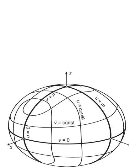
Figure 1: Coordinates on the ellipsoid.

In the domain where $u$ and $v$ are local coordinates the restriction of the initial system to the manifold $J_{h}$ admits the integrals

$$p_{u}^{2}+hU(u)=h\kappa,\qquad p_{v}^{2}-hV(v)=-h\kappa.$$ (2)

Denote by $J_{h,\kappa}$ the subset of $J_{h}$ defined by equations (2). The admissible values of $\kappa$ are $A\leqslant\kappa\leqslant C$. Let us find out the topological type of the integral manifolds $J_{h,\kappa}$ in the following cases: 1) $A\leqslant\kappa<B$; 2) $B<\kappa\leqslant C$; 3) $\kappa=B$.

Let $\mathfrak{W}={E}^{2}\setminus\{u=0\}$ and $\mathfrak{S}={E}^{2}\setminus\{v=n\}$ be the regions on the ellipsoid surface. In them, we introduce the local coordinates $\mathfrak{W}=\{(w,\varphi\,{\rm mod}\,4n)\}$, $\mathfrak{S}=\{(s,\theta\,{\rm mod}\,4m)\}$ similar to cylindrical ones putting

$$\begin{array}[]{cc}w=\begin{cases}u&\text{при $x\leqslant 0$;}\\ 2m-u&\text{при $x\geqslant 0$,}\\ \end{cases}&s=\begin{cases}v&\text{при $z\leqslant 0$;}\\ -v&\text{при $z\geqslant 0$,}\\ \end{cases}\end{array}$$

$$\begin{array}[]{cc}\varphi=\begin{cases}v&\text{при $y\geqslant 0,z\geqslant 0$;}\\ 2n-v&\text{при $y\leqslant 0,z\geqslant 0$;}\\ 2n+v&\text{при $y\leqslant 0,z\leqslant 0$;}\\ 4n-v&\text{при $y\geqslant 0,z\leqslant 0$,}\\ \end{cases}&\theta=\begin{cases}u&\text{при $x\geqslant 0,y\geqslant 0$;}\\ 2m-u&\text{при $x\leqslant 0,y\geqslant 0$;}\\ 2m+u&\text{при $x\leqslant 0,y\leqslant 0$;}\\ 4m-u&\text{при $x\geqslant 0,y\leqslant 0$.}\\ \end{cases}\end{array}$$

It is easily shown that these coordinates are compatible with the smooth structure of the ellipsoid.

Let us consider the cases 1 – 3.

If $A\leqslant\kappa<B$, then the motion takes place in the region $\mathfrak{W}$ and the equations admit the first integrals

$$H_{w}=p_{w}^{2}+hW(w)=h\kappa,\qquad H_{\varphi}=p_{\varphi}^{2}-h\Phi(\varphi)=-h\kappa,$$ (3)

where $W(w)=U(u(w))$, $\Phi(\varphi)=V(v(\varphi))$. The qualitative picture of the functions $W$ and $\Phi$ is shown in Fig. 2. In Fig. 3, we show the phase portraits of one-dimensional systems corresponding to the Hamilton functions $H_{w}$ and $H_{\varphi}$. Each manifold $J_{h,\kappa}$ is the product of level lines of the functions $H_{w}$ and $H_{\varphi}$ defined by (3). Thus, $J_{h,A}$ is two non-intersecting circles (they correspond to the cross section of the ellipsoid by the plane $x=0$ with two different directions of motion). If $A<\kappa<B$, then $J_{h,\kappa}$ consists of two two-dimensional tori each of which concentrically envelopes one of the circles out of $J_{h,A}$.

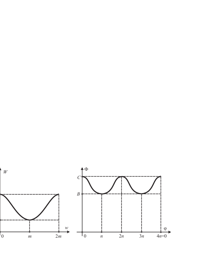
Figure 2: The functions $W$ and $\Phi$.

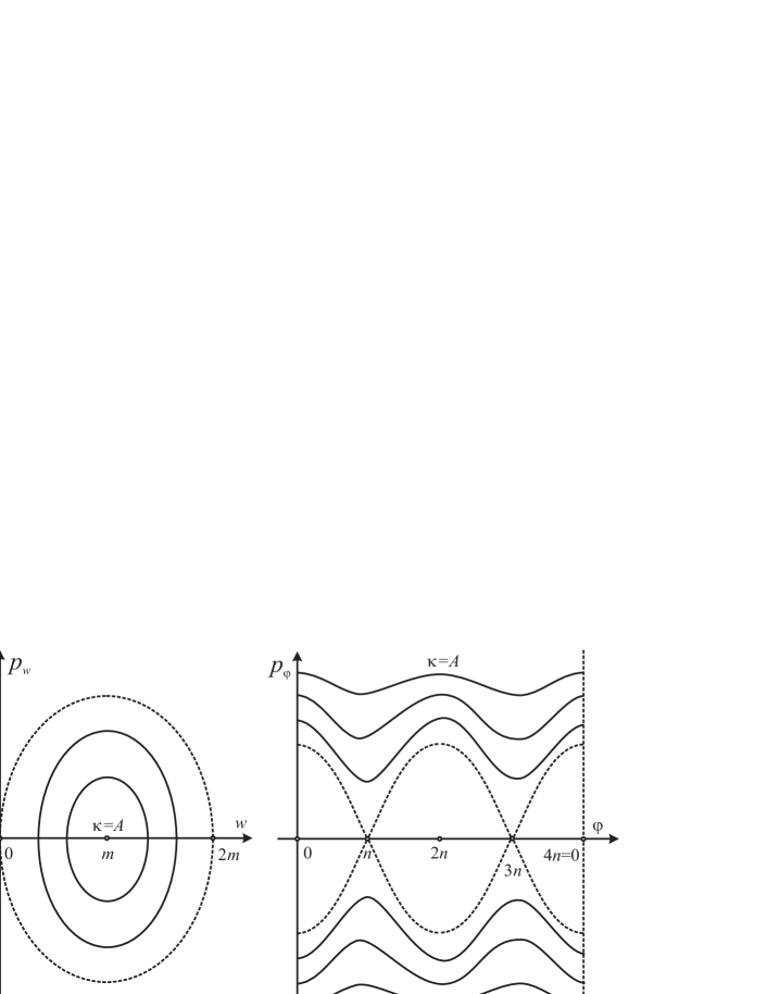
Figure 3: The portraits of one-dimensional systems.

In the case $B<\kappa\leqslant C$ the motion takes place in the region $\mathfrak{S}$. In $T^{*}\mathfrak{S}\cap J_{h}$ the integrals are defined

$$H_{s}=p_{s}^{2}-hS(s)=-h\kappa,\qquad H_{\theta}=p_{\theta}^{2}+h\Theta(\theta)=h\kappa,$$

where $S(s)=V(v(s))$, $\Theta(\theta)=U(u(\theta))$; the system splits into two one-dimensional ones. The manifold $J_{h,C}$ consists of two non-intersecting circles and $J_{h,\kappa}$ for $B<\kappa<C$ consists of two two-dimensional tori each of which concentrically envelopes one of the circles out of $J_{h,C}$.

In Fig. 4, where the diametrically opposite points of the ball boundary are identified, we show the sets corresponding to the manifolds $J_{h,A}$ and $J_{h,C}$ under the homeomorphism $\beta:P\to J_{h}$. The union of the circles 1 and 2 is the set $\beta^{-1}(J_{h,C})$. The set $\beta^{-1}(J_{h,A})$ consists of the circles 3 and 4.

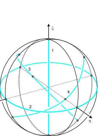
Figure 4: The integral circles.

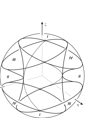
Figure 5: The tori regions.

Now let us consider the case $\kappa=B$. We denote by $K_{1}$, $K_{2}$, $K_{3}$, and $K_{4}$ the umbilical points $(u=0,v=n)$ on the ellipsoid surface lying respectively in the regions $\{x>0,z>0\}$, $\{x<0,z>0\}$, $\{x<0,z<0\}$, and $\{x>0,z<0\}$.

Proposition 2.

The cross section of the ellipsoid by the plane $y=0$ is a closed geodesic of the metric $d\Sigma$. All geodesics starting from an umbilical point at $t=0$ meet simultaneously at the opposite umbilical point.

Proof.

Let us use the coordinates $(w,\varphi)$. Introducing the ‘‘reduced time’’ $\tau$ by the formula $d\tau=[\Phi(\varphi)-W(w)]^{-1}dt$ and using equations (3) with $\kappa=B$, we get the equations of geodesics in the form

$${\frac{dw}{d\tau}=\pm\sqrt{h(B-W(w))},\qquad\frac{d\varphi}{d\tau}=\pm\sqrt{h(\Phi(\varphi)-B)}.}$$ (4)

Denote

$${F(w,w_{0})=\int\limits_{w_{0}}^{w}\frac{dw}{\sqrt{h(B-W(w)})}},\quad\displaystyle{G(\varphi,\varphi_{0})=\int\limits_{\varphi_{0}}^{\varphi}\frac{d\varphi}{\sqrt{h(\Phi(\varphi)-B)}}}.$$

Let $w=f(\tau,w_{0})$ and $\varphi=g(\tau,w_{0})$ be the inverse for the dependencies $\tau=F(w,w_{0})$ and $\tau=G(\varphi,\varphi_{0})$ respectively. Equations (4) admit the solutions

$$\begin{array}[]{ll}\bigl{(}w\equiv 0,\varphi=g(\pm\tau,\varphi_{0})\bigr{)},&\bigl{(}w\equiv 2m,\varphi=g(\pm\tau,\varphi_{0})\bigr{)},\\ \bigl{(}w=f(\pm\tau,w_{0}),\varphi\equiv n\bigr{)},&\bigl{(}w=f(\pm\tau,w_{0}),\varphi\equiv 3n\bigr{)}.\end{array}$$

This proves the first statement.

Consider an arbitrary trajectory of equations (4) starting at a point $\{w_{0},\varphi_{0}\}$ not belonging to the cross section $y=0$. Let, for definition, this point lie in the first octant, i.e., $m<w_{0}<2m$, $0<\varphi_{0}<n$. The initial velocity may have four directions according to the choice of the signs in (4). Suppose, for example, that $\left.dw/d\tau\right|_{\tau=0}>0$, $\left.d\varphi/d\tau\right|_{\tau=0}>0$. Then (see Fig. 3) as $\tau\to+\infty$, the coordinates $w$ and $\varphi$ monotonously increase and $w\to 2m$, $\varphi\to n({\rm mod}\,4n)$. As $\tau\to-\infty$ we have monotonous decreasing $w\to 0$ and $\varphi\to-n({\rm mod}\,4n)$.

Therefore the chosen trajectory of (4) asymptotically approaches $K_{1}$ as $\tau\to+\infty$ and $K_{3}$ as $\tau\to-\infty$. Another possible cases of the inial directions are considered analogously.

So, since the geodesics starting at an umbilical point can correspond only to the value $\kappa=B$, each such geodesic meets the cross section $y=0$ for the first time at the opposite umbilical point.

Let $\gamma_{1}(t)$ and $\gamma_{2}(t)$ be two geodesics such that $\gamma_{1}(0)=\gamma_{2}(0)=K_{3}$. Suppose that some time value $t=t_{0}>0$ corresponds to the value $\tau=0$ of the ‘‘reduced time’’. Let $\gamma_{1}(t_{0})=(w_{1},\varphi_{1})$, $\gamma_{2}(t_{0})=(w_{2},\varphi_{2})$. Then the dependency of $\gamma_{1}$ on the ‘‘reduced time’’ is $w=f(\tau,w_{1})$, $\varphi=g(\tau,\varphi_{1})$, and the equations of $\gamma_{2}$ are $w=f(\tau,w_{2})$, $\varphi=g(\tau,\varphi_{2})$. Denote by $t_{1}$ and $t_{2}$ the minimal positive values of $t$ for which $\gamma_{1}(t_{1})=\gamma_{2}(t_{2})=K_{1}$. Then

$$t_{1}=\int\limits_{-\infty}^{+\infty}[\Phi(g(\tau,\varphi_{1}))-W(f(\tau,\varphi_{1}))]d\tau,$$ (5)

$$t_{2}=\int\limits_{-\infty}^{+\infty}[\Phi(g(\tau,\varphi_{2}))-W(f(\tau,\varphi_{2}))]d\tau.$$ (6)

The integrals in (5) and (6) converge since the metric $d\Sigma$ does not have singularities.

Let us show that $t_{1}=t_{2}$. For this purpose we use the obvious relations

$$f(\tau,w_{1})=f(\tau-F(w_{1},w_{2}),w_{2}),\qquad g(\tau,w_{1})=g(\tau-G(w_{1},w_{2}),w_{2})$$ (7)

and the following almost obvious statement. Suppose that for a function $\psi(\tau)$ $(-\infty<\tau<+\infty)$ there exists such a point $\tau_{0}$ that $\chi(\tau)=\psi(\tau+\tau_{0})$ is an even function. If the integral

$$\int\limits_{-\infty}^{+\infty}[\psi(\tau)-\psi(\tau+k)]d\tau,$$

with some constant $k$ converges, then it equals zero. Using (7), we transform (5) as follows

$$t_{1}=\int\limits_{-\infty}^{+\infty}[\Phi(g(\tau,\varphi_{2}))-W(f(\tau+G(\varphi_{2},\varphi_{1}))-F(w_{2},w_{1}),w_{2})]d\tau.$$

Then we subtract the equality (6):

$$t_{1}-t_{2}=\int\limits_{-\infty}^{+\infty}[W(f(\tau,w_{2}))-W(f(\tau+k,w_{2}))]d\tau.$$

Here

$$k=G(\varphi_{2},\varphi_{1})-F(w_{2},w_{1})$$

does not depend on $\tau$.

It is easy to check that $W(f(\tau,w_{2}))$ as a function of $\tau$ satisfies the condition of the just formulated statement. For this, it is sufficient to choose $\tau_{0}$ in such a way that $f(\tau_{0},w_{2})=m$. Consequently, $t_{1}=t_{2}$. The proposition is proved. ∎

Let us now describe the type of the set $J_{h,B}$. The curves $O_{i}=J_{h}\cap T_{K}^{*}{E}^{2}$ $(i=1,2,3,4)$ are topological circles. According to Proposition 2, all trajectories starting at $O_{1}$ simultaneously cross $O_{3}$ and simultaneously return to $O_{1}$. Therefore this family of trajectories fills a closed flow tube, i.e., they fill a two-dimensional torus $T_{1}$ in $J_{h}$. In the same way the family of geodesics crossing $K_{2}$ and $K_{4}$ fills a two-dimensional torus $T_{2}$ in $J_{h}$. The tori $T_{1}$ and $T_{2}$ intersect by two circles corresponding to the cross section of the ellipsoid by the plane $y=0$ with two deffirent directions of motion.

In Fig. 5, we show how the set $\beta^{-1}(J_{h,B})$ is embedded in $P$ (the diametrically opposite points of the ball boundary are identified). The regions $I-IV$ are filled with the one-parameter families of the integral tori enveloping concentrically the circles 1 – 4 respectively (see Fig. 4).

References

[1]Kharlamov M.P. Reduction in mechanical systems with symmetry // Mekh. Tverd. Tela. – 1976. – N 8. – P. 4–18. arXiv:1401.4393.