CERN-PH-TH/2014-119

Magnetization of fluid phonons

and large-scale curvature perturbations

Massimo Giovannini

Department of Physics, Theory Division, CERN, 1211 Geneva 23, Switzerland
INFN, Section of Milan-Bicocca, 20126 Milan, Italy

Abstract

The quasinormal mode of a gravitating and magnetized fluid in a spatially flat, isotropic and homogeneous cosmological background is derived in the presence of the fluid sources of anisotropic stress and of the entropic fluctuations of the plasma. The obtained gauge-invariant description involves a system of two coupled differential equations whose physical content is analyzed in all the most relevant situations. The Cauchy problem of large-scale curvature perturbations during the radiation dominated stage of expansion can be neatly formulated and its general solution is shown to depend on five initial data assigned when the relevant physical wavelengths are larger than the particle horizon. The consequences of this approach are explored.

1 Formulation of the problem and basic results

The presumed existence of large-scale magnetic fields prior to matter-radiation equality (see e.g. [1, 2]) affects the evolution of all the scalar inhomogeneities of the plasma. The discussion of this physical system is feasible but algebraically cumbersome. Part of the technical complication stems from the scalar nature of the problem involving, on equal footing, the curvature perturbations, the diverse sources of anisotropic stress and the entropic fluctuations of the medium. In this investigation we ought to propose a simpler but effective framework for solving the evolution and normalization of the magnetized curvature perturbations. This strategy shall also be applied to the generalized analysis of the Cauchy problem for large-scale curvature perturbations.

In a conformally flat and homogeneous background geometry the fluctuations of a gravitating, irrotational and relativistic fluid admit a normal mode that has been originally obtained and scrutinized by Lukash [3] (see also [4]) even prior to the actual formulation of the conventional inflationary paradigm and in the context of the pioneering analyses of the relativistic theory of large-scale inhomogeneities [5, 6]. If the gravitating fluid contains arbitrary sources of anisotropic stress and of entropy perturbations the system admits a quasinormal mode that reduces to the Lukash variable in the absence of all the supplementary contributions. The magnetized quasinormal mode turns out to be coupled to the evolution of the anisotropic stress. The two resulting equations form a self-contained system that shall be derived and solved hereunder in various physical situations.

In anticipation of the actual derivation, the evolution equation of the quasinormal mode can be written, in a globally neutral plasma, as:

$${\mathcal{R}}^{\prime\prime}+2\frac{z_{t}^{\prime}}{z_{t}}{\mathcal{R}}^{\prime}-c_{\mathrm{st}}^{2}\nabla^{2}{\mathcal{R}}={\mathcal{S}}_{{\mathcal{R}}}[z_{t},\,c_{\mathrm{st}}^{2};\delta_{s}\rho_{B},\,\delta_{s}\rho_{E},\,\Pi_{t},\,\delta p_{\mathrm{nad}}],$$ (1.1)

where ${\mathcal{S}}_{{\mathcal{R}}}[.\,.\,.]$ denotes the functional of the two homogeneous background fields $z_{t}(\tau)$ and $c_{\mathrm{t}}^{2}(\tau)$

$$z_{t}=\frac{a^{2}\sqrt{p_{t}+\rho_{t}}}{{\mathcal{H}}c_{\mathrm{st}}},\qquad c_{\mathrm{st}}^{2}=\frac{p_{t}^{\prime}}{\rho_{t}^{\prime}},$$ (1.2)

and of three inhomogeneous background fields, namely: (i) the total anisotropic stress $\Pi_{t}$; (ii) the electromagnetic energy density (denoted respectively by $\delta\rho_{B}$ and $\delta\rho_{E}$); (iii) the non-adiabatic fluctuation of the total pressure (i.e. $\delta p_{\mathrm{and}}$).

The limit ${\mathcal{S}}_{{\mathcal{R}}}[.\,.\,.]\to 0$ in Eq. (1.1) reproduces exactly the equation obeyed by the Lukash variable ${\mathcal{R}}$ (or $z_{t}\,{\mathcal{R}}$ as defined in [3, 4]). This variable coincides, in fact, with the curvature perturbation on comoving orthogonal hypersurfaces and it is invariant under infinitesimal coordinate transformations as required in the context of the Bardeen formalism [7]. In the absence of magnetic fields, subsequent analyses [8, 9] followed the same logic of [3] but in the case of scalar field matter. All the normal modes identified in [3, 4, 8, 9] are related to the (rescaled) curvature perturbations on comoving orthogonal hypersurfaces [10, 11].

(i) The first of the three inhomogeneous contributions appearing in Eq. (1.1) and mentioned after Eq. (1.2) is the total anisotropic stress which is given as the sum of all the anisotropic stresses of the system, namely the fluid and the electromagnetic parts:

$$\Pi_{t}(\vec{x},\tau)=\Pi_{f}(\vec{x},\tau)+\Pi_{B}(\vec{x},\tau)+\Pi_{E}(\vec{x},\tau).$$ (1.3)

(ii) The second inhomogeneous contribution is given by the electromagnetic inhomogeneities

$$\delta_{s}\rho_{B}(\vec{x},\tau)=\frac{B^{2}(\vec{x},\tau)}{4\pi a^{4}},\qquad\delta_{s}\rho_{E}(\vec{x},\tau)=\frac{E^{2}(\vec{x},\tau)}{4\pi a^{4}},$$ (1.4)

$$\nabla^{2}\Pi_{B}(\vec{x},\tau)=\partial_{i}\partial_{j}\Pi^{ij}_{(B)}(\vec{x},\tau),\qquad\nabla^{2}\Pi_{E}(\vec{x},\tau)=\partial_{i}\partial_{j}\Pi^{ij}_{(E)}(\vec{x},\tau).$$ (1.5)

For practical reasons it is convenient to introduce $\sigma_{E}$ and $\sigma_{B}$, namely the dimensionless counterpart of $\Pi_{E}$ and $\Pi_{B}$:

$$\Pi_{B}(\vec{x},\tau)=(p_{\gamma}+\rho_{\gamma})\sigma_{B}(\vec{x},\tau),\qquad\Pi_{E}(\vec{x},\tau)=(p_{\gamma}+\rho_{\gamma})\sigma_{E}(\vec{x},\tau),$$ (1.6)

where $p_{\gamma}$ and $\rho_{\gamma}$ are the pressures and energy density of the photon background.

(iii) Finally the third inhomogeneous contribution the source term appearing in Eq. (1.1) is the non-adiabatic pressure fluctuation $\delta p_{\mathrm{nad}}$ (see e.g. [15, 16]) that can be written as:

$$\delta p_{\mathrm{nad}}(\vec{x},\tau)=\sum_{\mathrm{ij}}\frac{\partial p_{\mathrm{t}}}{\partial\varsigma_{\mathrm{ij}}}\delta\varsigma_{\mathrm{ij}}(\vec{x},\tau)=\frac{1}{6{\mathcal{H}}\rho_{\mathrm{t}}^{\prime}}\sum_{\mathrm{ij}}\rho_{\mathrm{i}}^{\prime}\rho_{\mathrm{j}}^{\prime}(c_{\mathrm{si}}^{2}-c_{\mathrm{sj}}^{2}){\mathcal{S}}_{\mathrm{ij}}(\vec{x},\tau),\qquad{\mathcal{S}}_{\mathrm{ij}}(\vec{x},\tau)=\frac{\delta\varsigma_{\mathrm{ij}}(\vec{x},\tau)}{\varsigma_{\mathrm{ij}}},$$ (1.7)

where the indices i and j are not tensor indices but denote two generic species of the pre-equality plasma. Furthermore, in Eq. (1.7), $c_{\mathrm{si}}^{2}$ and $c_{\mathrm{sj}}^{2}$ are the sound speeds of two (generic) species of the plasma; $\delta\varsigma_{\mathrm{ij}}(\vec{x},\tau)$ is the fluctuation of the specific entropy computed for a given pair of species and ${\mathcal{S}}_{\mathrm{ij}}(\vec{x},\tau)$, as indicated, is the relative fluctuation of $\varsigma_{\mathrm{ij}}$. With the precisions of Eqs. (1.3), (1.4)–(1.6) and (1.7) the general form of ${\mathcal{S}}_{{\mathcal{R}}}(\vec{x},\tau)$ can be expressed as

$${\mathcal{S}}_{{\mathcal{R}}}(\vec{x},\tau)=\Sigma_{\mathcal{R}}^{\prime}+2\frac{z_{t}^{\prime}}{z_{t}}\Sigma_{\mathcal{R}}+\frac{3a^{4}}{z_{t}^{2}}\Pi_{t},$$ (1.8)

where the auxiliary quantity $\Sigma_{\mathcal{R}}(\vec{x},\tau)$ is given by:

$$\Sigma_{{\mathcal{R}}}(\vec{x},\tau)=-\frac{{\mathcal{H}}}{p_{t}+\rho_{t}}\delta p_{\mathrm{nad}}+\frac{{\mathcal{H}}}{p_{t}+\rho_{t}}\biggl{[}\biggl{(}c_{\mathrm{st}}^{2}-\frac{1}{3}\biggr{)}(\delta_{s}\rho_{E}+\delta_{s}\rho_{B})+\Pi_{t}\biggr{]}.$$ (1.9)

The result of Eq. (1.1) must be complemented by an equation for the anisotropic stress that only couples to the quasinormal mode. Consider, in this respect, the standard $\Lambda$CDM paradigm (where $\Lambda$ qualifies the dark energy component and CDM stands for the cold dark matter contribution). In this case the anisotropic stress of the fluid comes only from the neutrino sector. Defining therefore $\Pi_{f}=(p_{\nu}+\rho_{\nu})\sigma_{\nu}$ in Eq. (1.9) the evolution equation of $\sigma_{\nu}$ becomes

$$\sigma_{\nu}^{\prime\prime\prime}+\frac{8}{5}{\mathcal{H}}^{2}R_{\nu}\Omega_{R}\sigma_{\nu}^{\prime}-\frac{6}{7}\nabla^{2}\sigma_{\nu}^{\prime}-\frac{32a^{4}{\mathcal{H}}}{5c_{\mathrm{st}}^{2}z_{t}^{2}}\Pi_{t}=\frac{4z_{t}^{2}}{15\overline{M}_{\mathrm{P}}^{2}}\biggl{[}\biggl{(}\frac{{\mathcal{H}}}{a^{2}}\biggr{)}^{\prime}({\mathcal{R}}^{\prime}-\Sigma_{{\mathcal{R}}})+c_{\mathrm{st}}^{2}\biggl{(}\frac{{\mathcal{H}}}{a^{2}}\biggr{)}\nabla^{2}{\mathcal{R}}\biggr{]}$$ (1.10)

where $\Omega_{R}=\rho_{R}/\rho_{t}$ is the critical fraction of radiation; $R_{\nu}$ and $R_{\gamma}$ count the fraction of neutrinos and photons in the radiation plasma. Once $\delta_{s}\rho_{B}$ and $\Pi_{B}$ are given, Eqs. (1.1) and (1.10) form a closed and gauge-invariant system of equations that can be solved under various approximations.

The system of Eqs. (1.1) and (1.10) bears some analogy with the inhomogeneous evolution of two minimally coupled scalar fields in a conformally flat and homogeneous background: as in our case the dynamics is described in terms of two quasinormal mode that are promoted to the status of exact canonical variables when one of the two fields is absent (see, e.g. [12, 13, 14] and discussions therein). Here the situation is similar but also rather different insofar as Eqs. (1.1) and (1.10) are, respectively, second and third order partial differential equations. The present approach simplifies and improves former analytical and numerical discussions. For instance it was pointed out in [17] that large-scale magnetic fields affect the scalar modes of the plasma, modify the initial conditions of the Einstein-Boltzmann hierarchy and ultimately change the temperature and polarization anisotropies. The results of [17] motivate the actual determination of the magnetized temperature and polarization anisotropies [18]. After Refs. [17, 18] different groups pursued similar analyses (see [19] and [20] for an incomplete list of references). The present construction may also some relevance for neighbouring problems where the fluctuations of the anisotropic stress play a physical role [21].

This paper is organized as follows. In section 2 the synchronous gauge derivation will be presented. In section 3 the main results are derived along the perspective of the longitudinal gauge. The overall symmetries of the system are examined in section 4. Various analytic solutions are discussed in section 5. In section 6 the formalism is applied to the analysis of the Cauchy problem for large-scale curvature perturbations. The concluding remarks are collected in section 7.

2 Synchronous gauge derivation

We shall consider a spatially flat Friedmann-Robertson-Walker background in the conformal time parametrization; as already mentioned in section 1, the total energy density and pressure of the plasma shall be denoted by $\rho_{t}$ and $p_{t}$. With these conventions the evolution equations of the homogeneous background are:

$${\mathcal{H}}^{2}=\frac{8\pi G}{3}a^{2}\rho_{t},$$ (2.1)

$${\mathcal{H}}^{2}-{\mathcal{H}}^{\prime}=4\pi Ga^{2}(p_{t}+\rho_{t}),$$ (2.2)

$$\rho_{t}^{\prime}+3{\mathcal{H}}(\rho_{t}+p_{t})=0,$$ (2.3)

where ${\mathcal{H}}=a^{\prime}/a$; the Planck mass is defined as $8\pi G=1/\overline{M}_{\mathrm{P}}^{2}$. In the synchronous gauge the metric fluctuations are related to the anisotropic stress and to the curvature perturbations by the following relevant pair of equations [17, 18]:

$${\mathcal{R}}^{\prime}=\Sigma_{R}-\frac{a^{2}k^{2}\xi}{4\pi G{\mathcal{H}}z_{t}^{2}}+\frac{a^{2}(h+6\xi)^{\prime}}{8\pi Gz_{t}^{2}},$$ (2.4)

$$(h+6\xi)^{\prime\prime}+2{\mathcal{H}}(h+6\xi)^{\prime}-2k^{2}\xi=24\pi Ga^{2}\Pi_{t},$$ (2.5)

where $\Pi_{t}$ is the total anisotropic stress (already introduced in Eq. (1.3)) that will now be explicitly rewritten as

$$\Pi_{t}=\biggl{[}(p_{\nu}+\rho_{\nu})\sigma_{\nu}+(p_{\gamma}+\rho_{\gamma})\sigma_{B}\biggr{]}.$$ (2.6)

In Eq. (2.6) the only source of fluid anisotropic stress has been identified with the neutrinos that will be taken to be massless as in the vanilla $\Lambda$CDM paradigm (see e.g. [22, 23] and discussions therein).

2.1 Evolution of the quasinormal mode

Moving $\Sigma_{{\mathcal{R}}}$ at the left hand side of Eq. (2.4) and taking the first time derivative of both sides of the obtained equation, the following result can easily be derived:

$$({\mathcal{R}}^{\prime}-\Sigma_{{\mathcal{R}}})^{\prime}+2\frac{z_{t}^{\prime}}{z_{t}}({\mathcal{R}}^{\prime}-\Sigma_{{\mathcal{R}}})=\frac{3a^{4}\Pi_{t}}{z_{t}^{2}}-\frac{k^{2}a^{2}\xi}{4\pi Gz_{t}^{2}}-\frac{a^{2}k^{2}\xi^{\prime}}{4\pi G{\mathcal{H}}z_{t}^{2}}+\frac{a^{2}k^{2}{\mathcal{H}}^{\prime}\xi}{4\pi G{\mathcal{H}}^{2}z_{t}^{2}}.$$ (2.7)

In Eq. (2.7) the expressions containing $(h+6\xi)^{\prime\prime}$ and $(h+6\xi)^{\prime}$ (arising as a result of the explicit derivation of both sides of Eq. (2.4)) have been eliminated by using Eq. (2.5) in combination with Eq. (2.4). Recalling then the synchronous gauge expression for the curvature perturbations on comoving orthogonal hypersurfaces, i.e.

$${\mathcal{R}}=\xi+\frac{{\mathcal{H}}\,\xi^{\prime}}{{\mathcal{H}}^{2}-{\mathcal{H}}^{\prime}},$$ (2.8)

Eq. (2.7) can be expressed, after some algebraic manipulations, as:

$$({\mathcal{R}}^{\prime}-\Sigma_{{\mathcal{R}}})^{\prime}+2\frac{z_{t}^{\prime}}{z_{t}}({\mathcal{R}}^{\prime}-\Sigma_{{\mathcal{R}}})+c_{\mathrm{st}}^{2}k^{2}{\mathcal{R}}=\frac{3a^{4}}{z_{t}^{2}}\Pi_{t},$$ (2.9)

which is nothing but the result anticipated in Eqs. (1.1) (see also Eqs. (1.8)–(1.9)) and now explicitly derived in Fourier space.

2.2 Evolution of the anisotropic stress

The equation for $\sigma_{\nu}$ can be written, in the synchronous gauge, as

$$\sigma_{\nu}^{\prime}=\frac{4}{15}\theta_{\nu}-\frac{3}{10}k{\mathcal{F}}_{\nu\,3}-\frac{2}{15}(h+6\xi)^{\prime},$$ (2.10)

where, following the standard conventions (see e.g. [17, 18]), $\theta_{\nu}$ and $\delta_{\nu}$ are, respectively, the divergence of the three-velocity of the neutrinos and the corresponding density contrast all computed in the synchronous gauge; ${\mathcal{F}}_{\nu\,3}$ is the octupole of the neutrino phase-space distribution. After taking the first time derivative of both sides of Eq. (2.10), the equations of the lower multipoles:

$$\delta_{\nu}^{\prime}=-\frac{4}{3}\theta_{\nu}+\frac{2}{3}h^{\prime},$$ (2.11)

$$\theta_{\nu}^{\prime}=\frac{k^{2}}{4}\delta_{\nu}-k^{2}\sigma_{\nu},$$ (2.12)

$${\mathcal{F}}_{\nu\ell}^{\prime}=\frac{k}{2\ell+1}[\ell{\mathcal{F}}_{\nu(\ell-1)}-(\ell+1){\mathcal{F}}_{\nu(\ell+1)}],\qquad\ell\geq 3,$$ (2.13)

can be used in the obtained result. We shall now assume that ${\mathcal{F}}_{\nu\ell}=0$ for all $\ell\geq 3$, i.e. ${\mathcal{F}}_{\nu\,3}=0$ but, according to Eq. (2.13), ${\mathcal{F}}_{\nu 3}^{\prime}\neq 0$. Recalling that ${\mathcal{F}}_{\nu 2}=2\sigma_{\nu}$ and using Eqs. (2.12) and (2.13), the first derivative of both sides of Eq. (2.10) implies:

$$\sigma^{\prime\prime}=\frac{k^{2}}{15}\delta_{\nu}-\frac{11}{21}k^{2}\sigma_{\nu}-\frac{2}{15}(h+6\xi)^{\prime\prime}.$$ (2.14)

We can take a further time derivative of both sides of Eq. (2.14) and insert Eq. (2.11) into the obtained expression. Equation (2.10) is subsequently used to get rid of $\theta_{\nu}$. The overall result of this procedure leads to the following intermediate equation:

$$\sigma_{\nu}^{\prime\prime\prime}+\frac{6}{7}k^{2}\sigma_{\nu}^{\prime}+\frac{4}{15}k^{2}\,\xi^{\prime}+\frac{2}{15}(h+6\xi)^{\prime\prime\prime}=0.$$ (2.15)

In Eq. (2.15) the term $(h+6\xi)^{\prime\prime\prime}$ is eliminated through the relation obtainable from the derivative of both sides of Eq. (2.5). Similarly the term $(h+6\xi)^{\prime\prime}$ can be replaced by using, again, Eq. (2.5) in its current form. We can finally trade the remaining term (i.e. $(h+6\xi)^{\prime}$ ) for ${\mathcal{R}}$ and its derivative by inverting Eq. (2.4), i.e.

$$(h+6\xi)^{\prime}=\frac{8\pi Gz_{t}^{2}}{a^{2}}({\mathcal{R}}^{\prime}-\Sigma_{{\mathcal{R}}})+\frac{2k^{2}\xi}{{\mathcal{H}}}.$$ (2.16)

The final equation we are looking for is thus given by:

$$\sigma_{\nu}^{\prime\prime\prime}+\frac{8}{5}{\mathcal{H}}^{2}R_{\nu}\Omega_{R}\sigma_{\nu}^{\prime}+\frac{6}{7}k^{2}\sigma_{\nu}^{\prime}-\frac{32}{5}{\mathcal{H}}^{3}R_{\nu}\Omega_{R}\biggl{(}\sigma_{\nu}+\frac{R_{\gamma}}{R_{\nu}}\sigma_{B}\biggr{)}$$

$$=\frac{8}{15c_{\mathrm{st}}^{2}}\biggl{(}{\mathcal{H}}-\frac{{\mathcal{H}}^{\prime}}{{\mathcal{H}}}\biggr{)}\biggl{(}\frac{{\mathcal{H}}^{\prime}}{{\mathcal{H}}}-2{\mathcal{H}}\biggr{)}({\mathcal{R}}^{\prime}-\Sigma_{{\mathcal{R}}})+\frac{8}{15}\biggl{(}\frac{{\mathcal{H}}^{\prime}}{{\mathcal{H}}}-{\mathcal{H}}\biggr{)}\,k^{2}{\mathcal{R}},$$ (2.17)

where $\Omega_{R}=\rho_{R}/\rho_{t}$ is the critical fraction of radiation; as anticipated $R_{\nu}$ and $R_{\gamma}$ count the fraction of neutrinos and photons in the radiation plasma.

Equation (2.17) can be formally written in different ways using the relations holding among the homogeneous background fields. In particular, from the definition of $z_{t}$ the following simple identity can be easily derived thanks to Eqs. (2.1) and (2.2):

$$\biggl{(}{\mathcal{H}}-\frac{{\mathcal{H}}^{\prime}}{{\mathcal{H}}}\biggr{)}=\frac{4\pi Gc_{\mathrm{st}}^{2}{\mathcal{H}}}{a^{2}}z_{t}^{2}.$$ (2.18)

Inserting Eq. (2.18) into Eq. (2.17) we obtain the wanted form of the equation which is the Fourier space version of the one already mentioned in Eq. (1.10)

$$\sigma_{\nu}^{\prime\prime\prime}+\frac{8}{5}{\mathcal{H}}^{2}R_{\nu}\Omega_{R}\sigma_{\nu}^{\prime}+\frac{6}{7}k^{2}\sigma_{\nu}^{\prime}-\frac{32}{5}{\mathcal{H}}^{3}R_{\nu}\Omega_{R}\biggl{(}\sigma_{\nu}+\frac{R_{\gamma}}{R_{\nu}}\sigma_{B}\biggr{)}$$

$$=\frac{32\pi G}{15}z_{t}^{2}\biggl{[}\biggl{(}\frac{{\mathcal{H}}}{a^{2}}\biggr{)}^{\prime}({\mathcal{R}}^{\prime}-\Sigma_{{\mathcal{R}}})-\frac{k^{2}c_{\mathrm{st}}^{2}{\mathcal{H}}}{a^{2}}{\mathcal{R}}\biggr{]},$$ (2.19)

recall, in fact, that within the notations established after Eq. (2.3) $8\pi G=1/\overline{M}_{\mathrm{P}}^{2}$.

Equations (2.9) and (2.17) have three relevant properties: they are exact to linear order, they are explicitly invariant under infinitesimal coordinate transformations and they are decoupled from all the remaining equations (even if coupled between them). To appreciate the importance of the three aforementioned properties it is useful to mention that one can easily obtain equations that are neither gauge-invariant nor exact to linear order. An example is, for instance, the following equation

$$\sigma_{\nu}^{\prime\prime}+2{\mathcal{H}}\sigma_{\nu}^{\prime}+\frac{4}{15}k^{2}\xi+\frac{8}{5}{\mathcal{H}}^{2}\Omega_{R}R_{\nu}\biggl{[}\sigma_{\nu}+\frac{R_{\gamma}}{R_{\nu}}\sigma_{B}\biggr{]}\simeq 0.$$ (2.20)

First, in Eq. (2.20) $\sigma_{\nu}$ is gauge-invariant but $\xi$ is not: then the whole equation does change for infinitesimal coordinate transformations. Second, Eq. (2.20) is derived by postulating that $\theta_{\nu}\ll\sigma_{\nu}^{\prime}$; the latter requirement is not satisfied by the standard adiabatic solution and it is therefore questionable. Equation (2.20) and other similar equations are not appropriate for the present approach which rests on the validity of Eqs. (2.9) and (2.17).

We finally remark that the potential ambiguities arising in the synchronous gauge [26] (see also [27]) play no role in the present derivation since we are just using the synchronous coordinate to compute a set of equations that are, ultimately, gauge-invariant. Furthermore, as already remarked in the past [17, 18] the synchronous gauge (together with the uniform cirvature gauge [12, 13]) is more suitable for the description of the modes with potentially relevant anisotropic stresses.

3 Longitudinal gauge derivation

Since Eqs. (2.9) and (2.17) are ultimately gauge-invariant they can be obtained in any other gauge. Let us consider, for simplicity, the conformally Newtonian gauge. While the longitudinal analysis is presented as a useful cross-check, the synchronous description is probably the most suitable, as already stressed at the end of the previous section.

3.1 Evolution of the quasinormal mode

Let us start by recalling that the relation between the curvature perturbations on comoving orthogonal hypersurfaces and the longitudinal degrees of freedom of the metric [7] is given by (see e.g. [17, 18] and also [12, 13, 14] for slightly different notations):

$${\mathcal{R}}=-\psi-\frac{{\mathcal{H}}({\mathcal{H}}\phi+\psi^{\prime})}{{\mathcal{H}}^{2}-{\mathcal{H}}^{\prime}},$$ (3.1)

$${\mathcal{R}}^{\prime}=\Sigma_{{\mathcal{R}}}+\frac{a^{2}k^{2}\psi}{4\pi G{\mathcal{H}}z_{t}^{2}}.$$ (3.2)

We follow here a procedure that is similar to the one already discussed in section 2. Thus, the equation for the quasinormal mode is obtained by deriving both sides of Eq. (3.2) and by using, in the obtained expression, Eqs. (3.1) and (3.2). The result of this manipulation is

$${\mathcal{R}}^{\prime\prime}+2\frac{z_{t}^{\prime}}{z_{t}}{\mathcal{R}}^{\prime}=\Sigma_{{\mathcal{R}}}^{\prime}+2\frac{z_{t}^{\prime}}{z_{t}}\Sigma_{{\mathcal{R}}}-\frac{a^{2}k^{2}({\mathcal{H}}^{2}-{\mathcal{H}}^{\prime})}{4\pi G{\mathcal{H}}z_{t}^{2}}{\mathcal{R}}+\frac{k^{2}a^{2}{\mathcal{H}}}{4\pi G{\mathcal{H}}z_{t}^{2}}(\psi-\phi).$$ (3.3)

In the longitudinal gauge the total anisotropic stress accounts for the mismatch between the two longitudinal fluctuations of the metric. In Fourier space we have

$$k^{2}(\phi-\psi)=-12\pi Ga^{2}[(p_{\nu}+\rho_{\nu})\sigma_{\nu}+(p_{\gamma}+\rho_{\gamma})\sigma_{B}].$$ (3.4)

Inserting Eq. (3.4) into Eq. (3.3) the obtained result coincides, as expected, with Eq. (2.9).

3.2 Evolution of the anisotropic stress

Assuming, as in section 2, that the whole anisotropic stress of the fluid comes from the neutrino sector, the lowest multipoles of the neutrino hierarchy read, in the longitudinal gauge,

$$\overline{\delta}_{\nu}^{\prime}=-\frac{4}{3}\overline{\theta}_{\nu}+4\psi^{\prime},$$ (3.5)

$$\overline{\theta}_{\nu}^{\prime}=\frac{k^{2}}{4}\overline{\delta}_{\nu}-k^{2}\sigma_{\nu}+k^{2}\phi,$$ (3.6)

$$\sigma_{\nu}^{\prime}=\frac{4}{15}\overline{\theta}_{\nu}-\frac{3}{10}k{\mathcal{F}}_{\nu 3}.$$ (3.7)

In Eqs. (3.5), (3.6) and (3.7) the overline has been used to stress that the corresponding quantities (unlike the ones of the previous section) are evaluated in the longitudinal gauge; $\sigma_{\nu}$ and ${\mathcal{F}}_{\nu\,3}$ do not have a the overline since they are both invariant under infinitesimal coordinate transformations; the higher multipoles (i.e. $\ell\geq 3$) are also gauge-invariant and obey the same equation already reported in section 2 (see, in particular, Eq. (2.13)).

Following the same procedure already outlined in the synchronous coordinate system, we take the conformal time derivative of both sides of Eq. (3.7); we thus obtain the analog of Eq. (2.14):

$$\sigma_{\nu}^{\prime\prime}=\frac{k^{2}}{15}\overline{\delta}_{\nu}+\frac{4}{15}k^{2}\phi-\frac{11}{21}k^{2}\sigma_{\nu},$$ (3.8)

where the neutrino hierarchy has been truncated, for illustration, to the octupole (notice, however, that ${\mathcal{F}}_{\nu\,3}^{\prime}\neq 0$). From Eq. (3.8) it also follows that:

$$\sigma_{\nu}^{\prime\prime\prime}+\frac{6}{7}k^{2}\sigma_{\nu}^{\prime}=\frac{4k^{2}}{15}(\phi-\psi)^{\prime}+\frac{8}{15}k^{2}\psi^{\prime}.$$ (3.9)

In Eq. (3.9) the term $k^{2}(\phi-\psi)^{\prime}$ can be replaced by taking the derivative of both sides of Eq. (3.4); the other term appearing at the right hand side of Eq. (3.9) is instead replaced by taking the derivative of Eq. (3.2) and by inserting, in the obtained expression, the decoupled equation for ${\mathcal{R}}$, i.e. Eq. (2.9). The result in terms of $k^{2}\psi^{\prime}$ becomes:

$$k^{2}\psi^{\prime} = \frac{1}{c_{\mathrm{st}}^{2}}\biggl{(}{\mathcal{H}}-\frac{{\mathcal{H}}^{\prime}}{{\mathcal{H}}}\biggl{)}(\frac{{\mathcal{H}}^{\prime}}{{\mathcal{H}}}-2{\mathcal{H}})({\mathcal{R}}^{\prime}-\Sigma_{{\mathcal{R}}})$$ (3.10)

$$+ 6{\mathcal{H}}^{3}\Omega_{R}R_{\nu}\biggl{(}\sigma_{\nu}+\frac{R_{\gamma}}{R_{\nu}}\sigma_{B}\biggr{)}-\biggl{(}{\mathcal{H}}-\frac{{\mathcal{H}}^{\prime}}{{\mathcal{H}}}\biggr{)}k^{2}{\mathcal{R}}.$$

Inserting Eq. (3.10) inside Eq. (3.9) and eliminating $k^{2}(\phi-\psi)^{\prime}$ with the derivative of Eq. (3.4) we obtain the equation already reported in Eqs. (2.17) and coinciding, after some algebra, with the result mentioned in Eq. (1.10) if the background relations discussed in Eq. (2.19) are used.

We conclude this section by recalling that another practical gauge where the derivation can be swiftly performed is the uniform curvature gauge [12, 13, 14] (see also [18] second paper). For reasons of space we shall not pursue this discussion here even if the general procedure will follow the general lines already discussed in the longitudinal and in the synchronous gauges.

4 Symmetries of the coupled system

The gauge-dependent derivations presented in sections 2 and 3 led to the gauge-invariant result anticipated in Eqs. (1.1) and (1.10). The same conclusion could be reached through a formalism that is explicitly gauge-invariant at every step. The second issue addressed hereunder involves the possibility of replacing ${\mathcal{R}}$ with different gauge-invariant variables related to it via the Hamiltonian constraint. It will be argued that this strategy is inconvenient. Towards the end of the section we shall focus on the dynamical symmetries of the gauge-invariant system and suggest possible generalizations.

4.1 Gauge-invariant derivations

The essentials of a fully gauge-invariant derivation are immediate in the light of the results of section 3. It suffices to recall, in fact, that in the general situation (and in Fourier space), the scalar fluctuations of the four-dimensional metric are parametrized by four different functions:

$$\delta_{s}g_{00}(k,\tau) = 2a^{2}(\tau)\,\phi(k,\tau),\qquad\delta_{s}g_{0i}(k,\tau)=ia^{2}k_{i}\,\beta(k,\tau),$$

$$\delta_{s}g_{ij}(k,\tau) = 2a^{2}(\tau)\,[\psi(k,\tau),\delta_{ij}+k_{i}\,k_{j}\,\alpha(k,\tau)],$$ (4.1)

where, as already mentioned, $\delta_{s}$ denotes the scalar mode of the corresponding perturbed entry. For infinitesimal coordinate shifts $\tau\to\widetilde{\tau}=\tau+\epsilon_{0}$ and ${x}^{i}\to\widetilde{x}^{i}=x^{i}+\partial^{i}\epsilon$ the functions $\phi(k,\tau)$, $\beta(k,\tau)$, $\psi(k,\tau)$ and $\alpha(k,\tau)$ introduced in Eq. (4.1) transform as:

$$\phi\to\widetilde{\phi}=\phi-{\mathcal{H}}\,\epsilon_{0}-\epsilon_{0}^{\prime},\qquad\psi\to\widetilde{\psi}=\psi+{\mathcal{H}}\,\epsilon_{0},$$ (4.2)

$$\beta\to\widetilde{\beta}=\beta+\epsilon_{0}-\epsilon^{\prime},\qquad\alpha\to\widetilde{\alpha}=\alpha-\epsilon.$$ (4.3)

Equations (2.9) and (2.19) (or, which is the same, Eqs. (1.1) and (1.10)) are derivable in a formalism that is gauge-invariant at every step by appealing to the properties of the two Bardeen potentials [7] which are constructed from the fluctuations of Eq. (4.1) and are given by:

$$\Phi=\phi+{\mathcal{H}}(\beta-\alpha^{\prime})+(\beta-\alpha^{\prime})^{\prime},\qquad\Psi=\psi-{\mathcal{H}}(\beta-\alpha^{\prime}).$$ (4.4)

In the longitudinal gauge $\Psi\equiv\psi$ and $\Phi\equiv\phi$. This means that the equations obeyed by the Bardeen potentials have, by definition, the same form of the equations written in the longitudinal gauge. Therefore the wanted gauge-invariant derivation will be exactly the one already presented in the case of the conformally Newtonian gauge (see section 3) with the proviso that $\phi\to\Phi$ and $\psi\to\Psi$.

4.2 Different gauge-invariant variables

The second point we ought to discuss in the present section has to do with the possibility of finding other gauge-invariant variables that could play effectively the role of ${\mathcal{R}}$. In terms of $\Phi$ and $\Psi$ and in real space the Hamiltonian constraint reads

$$\nabla^{2}\Psi-3{\mathcal{H}}({\mathcal{H}}\Phi+\Psi^{\prime})=4\pi Ga^{2}(\delta_{s}\rho_{t}+\delta_{s}\rho_{B}+\delta_{s}\rho_{E}),$$ (4.5)

where we restored, for the sake of generality, the presence of the electric variables. Let us now recall that the curvature perturbations on comoving orthogonal hypersurfaces (i.e. ${\mathcal{R}}$) and the total density contrast on uniform curvature hypersurfaces (conventionally denoted by $\zeta$) are simply related as

$$\zeta={\mathcal{R}}+\frac{\nabla^{2}\Psi}{12\pi Ga^{2}(p_{t}+\rho_{t})}.$$ (4.6)

Equation (4.6) can be derived from Eq. (4.5) by recalling the gauge-invariant expression of ${\mathcal{R}}$ and $\zeta$ (see e. g. [23])

$${\mathcal{R}}=-\Psi-\frac{{\mathcal{H}}({\mathcal{H}}\Phi+\Psi^{\prime})}{{\mathcal{H}}^{2}-{\mathcal{H}}^{\prime}},\qquad\zeta=-\Psi-{\cal H}\frac{\delta_{s}\rho_{t}+\delta_{s}\rho_{B}+\delta_{s}\rho_{E}}{\rho_{\mathrm{t}}^{\prime}}.$$ (4.7)

where, as in Eq. (4.5), $\delta_{s}\rho_{t}$ denotes the gauge-invariant fluctuation of the total energy density. It can be shown, by direct calculation, that the exact equation obeyed by $\zeta$ is much more involved than the one obeyed by ${\mathcal{R}}$ even if the two equations coincide in the $k\to 0$ limit. The equation for $\zeta$ can still be written in a decoupled form but it contains also terms proportional to $1/[k^{2}+{\mathcal{H}}^{2}u(\tau)]$ where $u(\tau)$ generically represents a time dependent function parametrizing the dominant contribution in the $k\to 0$ limit. This aspect can be appreciated by noticing that:

$${\mathcal{R}}^{\prime}=\Sigma_{{\mathcal{R}}}-\frac{a^{2}\nabla^{2}\Psi}{4\pi G{\mathcal{H}}z_{t}^{2}}.$$ (4.8)

If we now use Eq. (4.6) to eliminate $\nabla^{2}\Psi$, we shall have that $\zeta$ is fully determined by ${\mathcal{R}}$, ${\mathcal{R}}^{\prime}$ and $\Sigma_{{\mathcal{R}}}$ according to the relation

$$\zeta={\mathcal{R}}+\frac{\Sigma_{\mathcal{R}}-{\mathcal{R}}^{\prime}}{3{\mathcal{H}}c_{\mathrm{st}}^{2}}.$$ (4.9)

Equation (4.9) quantifies the difference between $\zeta$ and ${\mathcal{R}}$. This difference depends on $\Sigma_{{\mathcal{R}}}$ and ${\mathcal{R}}^{\prime}$. It also suggests that $\zeta$ and ${\mathcal{R}}$ are not fully equivalent when $\Sigma_{{\mathcal{R}}}\neq 0$. If we ought to avoid approximations the best strategy is to compute ${\mathcal{R}}$ by solving Eq. (1.1); derive then ${\mathcal{R}}^{\prime}$ and finally obtain $\zeta$ from Eq. (4.9).

In summary we can say that there exist other variables that are equivalent to ${\mathcal{R}}$ in the large-scale limit. However the use of these variables is inconvenient since they obey more cumbersome equations. The best strategy is to compute ${\mathcal{R}}$ and then derive all the other gauge-invariant variables.

4.3 Symmetries and generalizations of the gauge-invariant system

Having discussed all the technical aspects of the derivation of our system of equations we shall now discuss tits dynamical symmetries. Let us therefore consider the case of the vanilla $\Lambda$CDM paradigm and write Eqs. (1.1) and (1.10) as:

$${\mathcal{R}}^{\prime\prime}+2\frac{z_{t}^{\prime}}{z_{t}}{\mathcal{R}}^{\prime}+k^{2}c_{\mathrm{st}}^{2}{\mathcal{R}}=\Sigma_{\mathcal{R}}^{\prime}+2\frac{z_{t}^{\prime}}{z_{t}}\Sigma_{\mathcal{R}}+\frac{4c_{\mathrm{st}}^{2}}{(1+w_{t})}R_{\nu}{\mathcal{H}}^{2}\Omega_{R}\biggl{(}\sigma_{\nu}+\frac{R_{\gamma}}{R_{\nu}}\sigma_{B}\biggr{)},$$ (4.10)

$$\sigma_{\nu}^{\prime\prime\prime}+\frac{8}{5}{\mathcal{H}}^{2}R_{\nu}\Omega_{R}\sigma_{\nu}^{\prime}+\frac{6}{7}k^{2}\sigma_{\nu}^{\prime}-\frac{32}{5}{\mathcal{H}}^{3}R_{\nu}\Omega_{R}\biggl{(}\sigma_{\nu}+\frac{R_{\gamma}}{R_{\nu}}\sigma_{B}\biggr{)}$$

$$=\frac{8}{15c_{\mathrm{st}}^{2}}\biggl{(}{\mathcal{H}}-\frac{{\mathcal{H}}^{\prime}}{{\mathcal{H}}}\biggr{)}\biggl{(}\frac{{\mathcal{H}}^{\prime}}{{\mathcal{H}}}-2{\mathcal{H}}\biggr{)}({\mathcal{R}}^{\prime}-\Sigma_{{\mathcal{R}}})+\frac{8}{15}\biggl{(}\frac{{\mathcal{H}}^{\prime}}{{\mathcal{H}}}-{\mathcal{H}}\biggr{)}\,k^{2}{\mathcal{R}};$$ (4.11)

Note that Eq. (4.11) coincides with Eq. (2.17) which has been rewritten here for convenience. For $k\to 0$ Eqs. (4.10) and (4.11) are left unchanged if

$$\Sigma_{{\mathcal{R}}}(k,\tau) \to \widetilde{\Sigma}_{{\mathcal{R}}}(k,\tau)=\Sigma_{{\mathcal{R}}}(k,\tau)+\frac{\partial{\mathcal{A}}_{1}}{\partial\tau},$$ (4.12)

$${\mathcal{R}}(k,\tau) \to \widetilde{{\mathcal{R}}}(k,\tau)={\mathcal{R}}(k,\tau)+{\mathcal{A}}_{1}(k,\tau).$$ (4.13)

In the $\Lambda$CDM case it is also easy to obtain the explicit equation for the total anisotropic stress by defining the shifted variable $\sigma_{t}$ and by recalling that $\sigma_{B}^{\prime}=0$ whenever the evolution of the magnetic field is frozen-in. Let us then present a general expression for the evolution of $\sigma_{t}$ recalling that, in our case, $\Pi_{t}=(p_{t}+\rho_{t})\sigma_{t}=(p_{\nu}+\rho_{\nu})\sigma_{\nu}+(p_{\gamma}+\rho_{\gamma})\sigma_{B}$. The equation for $\sigma_{t}$ becomes, in Fourier space,

$$\sigma_{t}^{\prime\prime\prime}+{\mathcal{M}}({\mathcal{H}},c_{\mathrm{st}}^{2})\sigma_{t}^{\prime\prime}+{\mathcal{N}}({\mathcal{H}},c_{\mathrm{st}}^{2},k)\sigma_{t}^{\prime}+{\mathcal{Q}}({\mathcal{H}},c_{\mathrm{st}}^{2},k)\sigma_{t}={\mathcal{P}}({\mathcal{H}},c_{\mathrm{st}}^{2},k)$$ (4.14)

where

$${\mathcal{M}}({\mathcal{H}},c_{\mathrm{st}}^{2}) = 3{\mathcal{H}}(1-3c_{\mathrm{t}}^{2}),$$

$${\mathcal{N}}({\mathcal{H}},c_{\mathrm{st}}^{2},k) = \frac{8}{5}{\mathcal{H}}^{2}R_{\nu}\Omega_{R}+3(1-3c_{\mathrm{st}}^{2})({\mathcal{H}}^{\prime}+{\mathcal{H}}^{2})+\frac{6}{7}k^{2},$$

$${\mathcal{Q}}({\mathcal{H}},c_{\mathrm{st}}^{2},k) = \frac{8}{5}{\mathcal{H}}^{3}R_{\nu}\Omega_{R}(1-3c_{\mathrm{st}}^{2})$$

$$+ 3{\mathcal{H}}(1-3c_{\mathrm{st}}^{2})\biggl{(}3{\mathcal{H}}^{\prime}+{\mathcal{H}}^{2}+\frac{{\mathcal{H}}^{\prime\prime}}{{\mathcal{H}}}\biggr{)}-\frac{96}{5}{\mathcal{H}}^{3}c_{\mathrm{st}}^{2},$$

$${\mathcal{P}}({\mathcal{H}},c_{\mathrm{st}}^{2},k) = \frac{4z_{t}^{2}\,c_{\mathrm{st}}^{2}}{5\overline{M}_{\mathrm{P}}^{2}}R_{\nu}\biggl{[}\biggl{(}\frac{{\mathcal{H}}}{a^{2}}\biggr{)}^{\prime}({\mathcal{R}}^{\prime}-\Sigma_{{\mathcal{R}}})-k^{2}c_{\mathrm{st}}^{2}\biggl{(}\frac{{\mathcal{H}}}{a^{2}}\biggr{)}\biggr{]}.$$ (4.15)

In the case of an exact radiation background we have that $3c_{\mathrm{st}}^{2}\to 1$ and

$${\mathcal{M}}({\mathcal{H}},c_{\mathrm{st}}^{2}) \to 0,$$

$${\mathcal{N}}({\mathcal{H}},c_{\mathrm{st}}^{2},k) \to \frac{8}{5}{\mathcal{H}}^{2}R_{\nu}\Omega_{R}+\frac{6}{7}k^{2},$$

$${\mathcal{Q}}({\mathcal{H}},c_{\mathrm{st}}^{2},k) \to -\frac{32}{5}{\mathcal{H}}^{3},$$

$${\mathcal{P}}({\mathcal{H}},c_{\mathrm{st}}^{2},k) \to \frac{4z_{t}^{2}}{15\overline{M}_{\mathrm{P}}^{2}}R_{\nu}\biggl{[}\biggl{(}\frac{{\mathcal{H}}}{a^{2}}\biggr{)}^{\prime}({\mathcal{R}}^{\prime}-\Sigma_{{\mathcal{R}}})-k^{2}c_{\mathrm{st}}^{2}\biggl{(}\frac{{\mathcal{H}}}{a^{2}}\biggr{)}\biggr{]}.$$ (4.16)

Further generalizations of our set of equations are possible but we shall not indulge in these details. We shall now focus on the physical properties of the analytical and numerical solutions of the system.

5 Analytic solutions

5.1 Preliminaries

Deep in the radiation-dominated epoch and for typical wavelengths larger than the Hubble radius (i.e. $k\tau\ll 1$) the total anisotropic stress should obey the conditions

$$\sigma_{t}(k,\tau)\ll 1,\qquad\sigma_{t}^{\prime}(k,\tau)\ll 1,\qquad\sigma_{t}^{\prime\prime}(k,\tau)\ll 1.$$ (5.1)

The conditions of Eq. (5.1) can be guessed from the known properties of the standard adiabatic solution [24] (see also [22, 23]). In the vanilla $\Lambda$CDM paradigm the dimensionless anisotropic stress is $\sigma_{t}=R_{\nu}\sigma_{\nu}$. Recalling the symmetries of Eqs. (4.12)–(4.13), in the magnetized $\Lambda$CDM paradigm (sometimes dubbed m$\Lambda$CDM) $\sigma_{t}=R_{\nu}\sigma_{\nu}+R_{\gamma}\sigma_{B}$.

The initial conditions for ${\mathcal{R}}(k,\tau)$ during the radiation-dominated phase can be bootstrapped from the inflationary solution:

$${\mathcal{R}}(k,\tau)\simeq{\mathcal{R}}_{*}(k)+\frac{1+\eta+\epsilon}{(3-\epsilon)}\biggl{(}\frac{z_{*}}{z_{t}}\biggr{)}^{2}\biggl{(}\frac{H_{*}a_{*}}{Ha}\biggr{)}{\mathcal{R}}_{*},$$ (5.2)

where the star denotes the time at which the given wavelength crossed the Hubble radius during inflation; in Eq. (5.2) $\epsilon=-\dot{H}/H^{2}$ and $\eta=\ddot{\varphi}/(H\dot{\varphi})$ are the two standard slow-roll parameters that we take to be constant, for simplicity. Assuming a sudden reheating approximation taking place at a typical conformal time-scale $\tau_{r}$ the solution for the evolution of the curvature perturbations with wavelength larger than the Hubble radius can be written, after some simple algebra:

$${\mathcal{R}}(k,\tau)={\mathcal{R}}_{*}(k)+\biggl{(}\frac{a_{r}}{a}\biggr{)}\frac{(1+\eta+\epsilon)(3+\eta+\epsilon)}{(3-\epsilon)}{\mathcal{R}}_{*}(k)\biggl{(}\frac{a_{*}\,H_{*}}{a_{r}\,H_{r}}\biggr{)}^{3}$$ (5.3)

To higher order in $k\tau$ the decaying mode practically does not affect the solution since it is strongly suppressed and the full solution can be parametrized as ${\mathcal{R}}(k,\tau)={\mathcal{R}}_{*}j_{0}(c_{\mathrm{st}}\,y)$ where $c_{\mathrm{st}}\simeq 1/\sqrt{3}$ is the sound speed during the radiation-dominated phase and $j_{0}(c_{\mathrm{st}}\,y)$ is the spherical Bessel function of zeroth order.

Equations (5.2) and (5.3) can be directly used as initial conditions of the subsequent evolution but they can also be simplified by just positing the constancy of ${\mathcal{R}}$ at large-scales. Again this is typical of the standard adiabatic solution incorporated in the $\Lambda$CDM paradigm but the general situation could be different. During the subsequent radiation epoch $c_{\mathrm{st}}=1/\sqrt{3}$, and the canonical form of Eqs. (4.10)–(4.14) can be directly written in terms $y=k\tau$:

$$\frac{d^{2}{\mathcal{R}}}{dy^{2}}+\frac{2}{y}\frac{d{\mathcal{R}}}{dy}+\frac{{\mathcal{R}}}{3}=\frac{1}{y}\biggl{(}\frac{d\sigma_{t}}{dy}+\frac{2}{y}\sigma_{t}\biggr{)},$$ (5.4)

$$\frac{d^{3}\sigma_{t}}{dy^{3}}+\biggl{(}\frac{6}{7}+\frac{8R_{\nu}}{5y^{2}}\biggr{)}\frac{d\sigma_{t}}{dy}-16\frac{R_{\nu}}{y^{3}}\sigma_{t}+\frac{16R_{\nu}}{5y^{2}}\biggl{(}3\frac{d{\mathcal{R}}}{dy}+\frac{y{\mathcal{R}}}{3}\biggr{)}=0.$$ (5.5)

The variable $y$ during the radiation epoch obeys the exact chain of equalities $y=k/{\mathcal{H}}=k/(aH)$ since, during radiation, ${\mathcal{H}}=1/\tau$. This means that $y$ can be viewed as the ratio between the particle horizon and the physical wavelength of the fluctuation. Equations (5.4)–(5.5) imply that the system depends on a single scaling variable.

5.2 Solutions in the radiation epoch

We look preliminarily for an approximate solution of Eqs. (5.4) and (5.5) in the limit $y<1$ and with the initial conditions of Eq. (5.1):

$$\sigma_{t}(y)={\mathcal{A}}y^{\gamma}+{\mathcal{O}}(y^{2+\gamma}),\qquad\gamma>0,$$

$${\mathcal{R}}(y)={\mathcal{R}}_{*}+{\mathcal{B}}y^{\delta}+{\mathcal{O}}(y^{2+\delta}),\qquad\delta>0.$$ (5.6)

Equations (5.4) and (5.5) imply that the parameters of Eq. (5.6) must obey the following relation:

$${\mathcal{A}}=\frac{18{\mathcal{B}}+{\mathcal{R}}_{*}}{12},\qquad\delta=\gamma=2.$$ (5.7)

The gauge-invariant solution of Eqs. (5.6)–(5.7) can be translated in any specific coordinate system and, in particular, in the conformally Newtonian gauge:

$$\frac{d{\mathcal{R}}}{dy}=\frac{\sigma_{t}}{y}+\frac{y\psi}{6},\qquad{\mathcal{R}}=-\psi-\frac{\phi}{2}.$$ (5.8)

Eq. (5.7) implies ${\mathcal{A}}=(\psi-\phi)/6$ where $\psi$ and $\phi$ are both constant to leading order: this is the standard result valid in the longitudinal gauge (see, e.g. [24, 25] and also [17, 18]). The same strategy can be used in the synchronous coordinate system. The full gauge-invariant solution for the magnetized adiabatic mode can be written explicitly as [17, 18]:

$${\mathcal{R}}(y) = {\mathcal{R}}_{*}+{\mathcal{B}}y^{2}+{\mathcal{O}}(y^{4}),$$

$$\sigma_{\nu}(y) = -\frac{R_{\gamma}}{R_{\nu}}\sigma_{B}+\frac{18{\mathcal{B}}+{\mathcal{R}}_{*}}{12}y^{2}+{\mathcal{O}}(y^{4}).$$ (5.9)

In the limit $\sigma_{B}\to 0$, the solution of Eq. (5.9) reproduces the standard adiabatic mode.

From the previous solution we can also derive the solution for $\zeta$; in fact Eq. (4.9) implies

$$\zeta(y)={\mathcal{R}}(y)+\sigma_{t}(y)-y\frac{d{\mathcal{R}}}{dy}\equiv{\mathcal{R}}_{*}+\frac{1}{2}\biggl{(}{\mathcal{B}}+\frac{{\mathcal{R}}_{*}}{6}\biggr{)}y^{2}+{\mathcal{O}}(y^{4}),$$ (5.10)

where the second equality follows after inserting the solution of Eq. (5.9) into the first relation of Eq. (5.10). If we take now the difference between $\zeta$ and ${\mathcal{R}}$ we correctly obtain the Hamiltonian constraint stipulating that

$$\zeta-{\mathcal{R}}=\frac{1}{2}\biggl{(}\frac{{\mathcal{R}}_{*}}{6}-{\mathcal{B}}\biggr{)}y^{2}\equiv-\frac{\psi_{*}}{6}y^{2}.$$ (5.11)

Since ${\mathcal{R}}(y)$ and $\sigma_{\nu}(y)$ are both gauge-invariant the explicit values of ${\mathcal{A}}$ and ${\mathcal{B}}$ are also gauge-invariant and can be determined in any gauge by demanding that the Hamiltonian and the momentum constraints are satisfied. Skipping the technical details the results of this analysis are:

$${\mathcal{A}}({\mathcal{R}}_{*},\,\Omega_{B},\,\sigma_{B}) = -\frac{2R_{\nu}{\mathcal{R}}_{*}}{3(15+4R_{\nu})}-\frac{R_{\gamma}\,R_{\nu}\,(R_{\nu}\Omega_{B}-4\sigma_{B})}{2R_{\nu}(15+4R_{\nu})},$$ (5.12)

$${\mathcal{B}}({\mathcal{R}}_{*},\,\Omega_{B},\,\sigma_{B}) = -\frac{(5+4R_{\nu}){\mathcal{R}}_{*}}{6(15+4R_{\nu})}-\frac{R_{\gamma}(R_{\nu}\Omega_{B}-4\sigma_{B})}{3(15+4R_{\nu})}.$$ (5.13)

The initial conditions during radiation can be fixed by demanding that the only source of anisotropic stress is provided by the magnetic fields. In this case the equation to integrate is simply given by:

$$\frac{d^{2}{\mathcal{R}}}{dy^{2}}+\frac{2}{y}\frac{dR}{dy}+c_{\mathrm{st}}^{2}{\mathcal{R}}=\frac{2R_{\gamma}\sigma_{B}}{y^{2}}.$$ (5.14)

Defining $q(y)=y{\mathcal{R}}(y)$ we get the following equation

$$\frac{d^{2}q}{dy^{2}}+c_{\mathrm{st}}^{2}q=\frac{2R_{\gamma}\sigma_{B}}{y},$$ (5.15)

whose general solution can be written as:

$$q(y)=C_{1}\cos{(c_{\mathrm{st}}y)}+C_{2}\sin{(c_{\mathrm{st}}y)}+\frac{2R_{\gamma}\sigma_{B}}{c_{\mathrm{st}}}\int_{y_{i}}^{y}\,\frac{\sin{[c_{\mathrm{st}}(y-\xi)]}}{\xi}\,d\xi.$$ (5.16)

In terms of ${\mathcal{R}}(y)$ the solution of Eq. (5.16) with the large-scale boundary conditions provided by the adiabatic mode can be written as

$${\mathcal{R}}(y) = {\mathcal{R}}_{*}\frac{\sin{(c_{\mathrm{st}}y)}}{c_{\mathrm{st}}y}$$ (5.17)

$$+ 2R_{\gamma}\sigma_{B}\biggl{[}\biggl{(}\mathrm{Ci}(c_{\mathrm{st}}y)-\mathrm{Ci}(c_{\mathrm{st}}y_{i})\biggr{)}\frac{\sin{(c_{\mathrm{st}}y)}}{c_{\mathrm{st}}y}$$

$$+ \biggl{(}\mathrm{Si}(c_{\mathrm{st}}y_{i})-\mathrm{Si}(c_{\mathrm{st}}y)\biggr{)}\frac{\cos{(c_{\mathrm{st}}y)}}{c_{\mathrm{st}}y}\biggr{]},$$

where

$$\mathrm{Ci}(z)=-\int_{z}^{\infty}\frac{\cos{t}}{t}\,dt,\qquad\mathrm{Si}(z)=\int_{0}^{z}\frac{\sin{t}}{t}\,dt.$$ (5.18)

The previous expression can be expanded in powers of $y$ and $y_{i}$ with the result that:

$${\mathcal{R}}(y)={\mathcal{R}}_{*}+2R_{\gamma}\sigma_{B}[\ln{(y/y_{i})}-1]+2R_{\gamma}\sigma_{B}y_{i}/y+{\mathcal{O}}(y^{2})+{\mathcal{O}}(y^{2}y_{i})+{\mathcal{O}}(y_{i}^{2})$$ (5.19)

where we recall that $y\geq y_{i}$. As we shall see in section 6 the purely magnetic initial conditions can be studied from the more general perspective of a consistent formulation of the Cauchy problem for the coupled evolution of the quasinormal mode and of the total anisotropic stress.

5.3 Matter-radiation transition

The equations for the curvature perturbations and for the shifted anisotropic stress can be written in the $\alpha$ paramerization where $\alpha=a/a_{eq}$ is the normalized scale factor. The exact solution of Friedmann equations (2.1)–(2.3) across the transition implies that $\alpha=(\tau/\tau_{1})^{2}+2(\tau/\tau_{1})$; $\tau_{1}=(\sqrt{2}+1)\tau_{eq}$ and $\tau_{eq}$ denotes the time of matter-radiation equality. In the $\alpha$ parametrization we have:

$$\tau_{1}\Sigma_{\mathcal{R}}(\alpha)=\frac{8\sqrt{\alpha+1}}{\alpha(3\alpha+4)}\biggl{[}\sigma_{t}-\frac{3\alpha\Omega_{B}R_{\gamma}}{4(3\alpha+4)}\biggr{]},$$

$$z_{t}^{2}(\alpha)=\frac{3}{4}\,\overline{M}_{P}^{2}\,a_{eq}^{2}\,\frac{\alpha^{2}(3\alpha+4)^{2}}{\alpha+1}.$$ (5.20)

The evolution equation of the quasinormal mode can be written as:

$$\frac{\partial^{2}{\mathcal{R}}}{\partial\alpha^{2}}+{\mathcal{Q}}_{1}(\alpha)\frac{\partial{\mathcal{R}}}{\partial\alpha}+{\mathcal{Q}}_{2}(\alpha)\kappa^{2}{\mathcal{R}}=\biggl{[}{\mathcal{Q}}_{3}(\alpha)\sigma_{t}+{\mathcal{Q}}_{4}(\alpha)\frac{\partial\sigma_{t}}{\partial\alpha}\biggr{]}-{\mathcal{Q}}_{5}(\alpha)R_{\gamma}\Omega_{B},$$ (5.21)

where the five background dependent functions of Eq. (5.21) are:

$${\mathcal{Q}}_{1}(\alpha) = \frac{21\alpha^{2}+36\alpha+16}{2\alpha(3\alpha+4)(\alpha+1)},\qquad{\mathcal{Q}}_{2}(\alpha)=\frac{1}{3(3\alpha+4)(\alpha+1)},$$

$${\mathcal{Q}}_{3}(\alpha) = \frac{2(9\alpha^{2}+24\alpha+16)}{\alpha^{2}(\alpha+1)(3\alpha+4)^{2}},\qquad{\mathcal{Q}}_{4}(\alpha)=\frac{4}{\alpha(3\alpha+4)},$$

$${\mathcal{Q}}_{5}(\alpha) = \frac{3}{2\alpha(\alpha+1)(3\alpha+4)}.$$ (5.22)

In the notations of Eq. (5.21), the equation obeyed by the shifted anisotropic stress is:

$$\frac{\partial^{3}\sigma_{t}}{\partial\alpha^{3}}+{\mathcal{U}}_{1}(\alpha)\frac{\partial^{2}\sigma_{t}}{\partial\alpha^{2}}+\biggl{[}{\mathcal{U}}_{2}(\alpha)+\kappa^{2}{\mathcal{U}}_{3}(\alpha)\biggr{]}\frac{\partial\sigma_{t}}{\partial\alpha}-{\mathcal{U}}_{4}(\alpha)\sigma_{t}=-\kappa^{2}{\mathcal{U}}_{5}(\alpha){\mathcal{R}}$$

$$-R_{\nu}{\mathcal{U}}_{6}(\alpha)\frac{\partial{\mathcal{R}}}{\partial\alpha}-{\mathcal{U}}_{7}(\alpha)R_{\nu}R_{\gamma}\Omega_{B},$$ (5.23)

where the background dependent functions are now defined as:

$${\mathcal{U}}_{1}(\alpha)=\frac{3}{2(\alpha+1)},\qquad{\mathcal{U}}_{2}(\alpha)=\frac{8}{5\alpha^{2}(\alpha+1)},$$

$${\mathcal{U}}_{3}(\alpha)=\frac{3}{14(\alpha+1)},\qquad{\mathcal{U}}_{4}(\alpha)=\frac{2(15\alpha^{2}+54\alpha+40)}{5\alpha^{3}(\alpha+1)^{2}},$$

$${\mathcal{U}}_{5}(\alpha)=\frac{(3\alpha+4)}{15\alpha(\alpha+1)^{2}},\qquad{\mathcal{U}}_{6}(\alpha)=\frac{(3\alpha+4)^{2}(5\alpha+6)}{10\alpha^{2}(\alpha+1)^{2}},$$

$${\mathcal{U}}_{7}(\alpha)=\frac{3(5\alpha+6)}{10\alpha^{2}(\alpha+1)^{2}}.$$ (5.24)

In the limit $\alpha\to 0$, the functions ${\mathcal{Q}}_{i}(\alpha)$ (with $i$ going from $1$ to $5$) and ${\mathcal{U}}_{j}(\alpha)$ (with $j$ going from $1$ to $7$) can be expanded and the resulting system of equations becomes:

$$\frac{\partial^{2}{\mathcal{R}}}{\partial\alpha^{2}}+\frac{2}{\alpha}\frac{\partial{\mathcal{R}}}{\partial\alpha}+\frac{\kappa^{2}}{12}{\mathcal{R}}=\biggl{[}\frac{2}{\alpha}\sigma_{t}+\frac{\partial\sigma_{t}}{\partial\alpha}\biggr{]}-\frac{3}{8\alpha}R_{\gamma}\Omega_{B},$$

$$\frac{\partial^{3}\sigma_{t}}{\partial\alpha^{3}}+\frac{3}{2}\frac{\partial^{2}\sigma_{t}}{\partial\alpha^{2}}+\biggl{[}\frac{8}{5\alpha^{2}}+\frac{3\kappa^{2}}{14}\biggr{]}\frac{\partial\sigma_{t}}{\partial\alpha}-\frac{16}{\alpha^{3}}R_{\nu}\sigma_{t}=-\frac{4\kappa^{2}}{15}R_{\nu}{\mathcal{R}}-\frac{48}{5\alpha^{2}}R_{\nu}\frac{\partial{\mathcal{R}}}{\partial\alpha}-\frac{9}{5\alpha^{2}}R_{\nu}R_{\gamma}\Omega_{B}.$$

It is clear that these equations coincide with the ones previously derived since $\kappa=k\tau_{1}$ and $\alpha\simeq 2\,\tau/\tau_{1}$. Note that the important terms containing $\Omega_{B}$ are suppressed: if we pass to the variable $\kappa\alpha=2y$ the terms containing $\Omega_{B}$ turn out to be suppressed as $\Omega_{M}/\Omega_{R}=\alpha$ (where as usual $\Omega_{M}=\rho_{M}/\rho_{t}$) in the limit $\alpha\to 0$.

6 Setting the large-scale initial conditions

6.1 Generalities

So far no attempt has been made to formulate the Cauchy problem of large-scale inhomogeneities solely on the basis of the system discussed in the present paper. To proceed along this direction, it is convenient to change the variable appearing in Eqs. (5.4) and (5.5) from $y$ to $x=\ln{y}$; with this change of variables the equations become:

$$\frac{d^{3}\sigma_{\mathrm{t}}}{dx^{3}}-3\frac{d^{2}\sigma_{\mathrm{t}}}{dx^{2}}+\biggl{(}\frac{8}{5}R_{\nu}+2+\frac{6}{7}e^{2x}\biggr{)}\frac{d\sigma_{\mathrm{t}}}{dx}=16R_{\nu}\sigma_{\mathrm{t}}-\frac{48R_{\nu}}{5}\biggl{(}\frac{d{\mathcal{R}}}{dx}+\frac{{\mathcal{R}}}{9}e^{2x}\biggr{)},$$ (6.1)

$$\frac{d^{2}{\mathcal{R}}}{dx^{2}}+\frac{d{\mathcal{R}}}{dx}+c_{\mathrm{st}}^{2}\,e^{2x}{\mathcal{R}}=\biggl{(}\frac{d\sigma_{\mathrm{t}}}{dx}+2\sigma_{\mathrm{t}}\biggr{)}.$$ (6.2)

Five initial conditions define the space of the Cauchy data of Eqs. (6.1)–(6.2): three initial data are related to Eq. (6.1) and two initial data must be specified in connection with Eq. (6.2). We shall use the following shorthand notation:

$$\sigma_{\mathrm{t}}(x_{i}),\qquad\sigma_{\mathrm{t}}^{\prime}(x_{i})=\frac{d\sigma_{\mathrm{t}}}{dx}\biggl{|}_{x=x_{i}},\qquad\sigma_{\mathrm{t}}^{\prime\prime}(x_{i})=\frac{d^{2}\sigma_{\mathrm{t}}}{dx^{2}}\biggl{|}_{x=x_{i}},$$ (6.3)

for the total anisotropic stress and its first two derivatives and

$${\mathcal{R}}(x_{i}),\qquad{\mathcal{R}}^{\prime}(x_{i})=\frac{d{\mathcal{R}}}{dx}\biggl{|}_{x=x_{i}},$$ (6.4)

for the curvature perturbations and its first derivative.

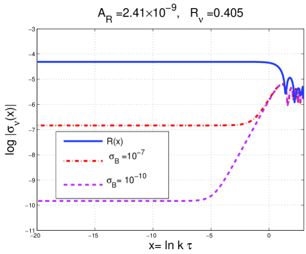
Figure 1: The standard adiabatic initial conditions of Eq. (6.5) are illustrated.

The initial data of Eqs. (6.3) and (6.4) are assigned when all the relevant wavelengths are larger than the Hubble radius during the radiation epoch. We define $x_{i}$ as the initial value of $x=\ln{k\tau}$. Notice that $x_{i}$ will typically be larger than one (in absolute value) and negative. This is because $k\tau=k/{\mathcal{H}}\ll 1$ for all the wavelengths larger than the Hubble radius. The large-scale power spectra of curvature are customarily assigned at a typical pivot scale $k_{\mathrm{p}}=0.002\,\mathrm{Mpc}^{-1}$ (see e.g. [28, 29]). The fiducial values of the cosmological parameters determined, for instance, by the WMAP collaboration [29] (see also [28]) imply $\tau_{eq}\simeq{\mathcal{O}}(120)\,\mathrm{Mpc}$ for the equality time already discussed at the end of section 5. Thus the maximal value of $x$ at equality be of the order of $\ln{(k_{\mathrm{p}}\,\tau_{\mathrm{eq}})}\sim-1.4$. The initial value of $x$ is much smaller. For instance, if $\tau$ coincides with the time of neutrino decoupling we will have that $k_{\mathrm{p}}\tau_{i}$ can easily be ${\mathcal{O}}(10^{-9})$ so that $x_{i}=\ln{k\tau_{i}}={\mathcal{O}}(-20)$. In the numerical examples discussed hereunder we shall always consider a fiducial interval of $x$ ranging from $-20$ to $3$. When $x$ is in the interval $-1.4<x<3$ the radiation phase is already replaced by the matter dominated epoch. Even of the physical range of $x$ goes from $-20$ to $-1.4$ we shall extend this range to positive values of $x$ and artificially assume a slightly longer duration of the radiation phase. This is done just to account graphically for the oscillating regime. The quantitative error due to the matter-radiation transition is immaterial for the present considerations but can become important if we ought to assess the magnetized observables of the Cosmic Microwave Background (see e.g. [17, 18]).

6.2 The conventional adiabatic paradigm

As already discussed in section 5 in the standard $\Lambda$CDM case the total anisotropic stress coincides with the neutrino component and in the language of Eqs. (6.3) and (6.4) the adiabatic initial conditions demand:

$${\mathcal{R}}(x_{i})={\mathcal{R}}_{*},\qquad{\mathcal{R}}^{\prime}(x_{i})=0,\qquad\sigma_{\mathrm{t}}(x_{i})=\sigma_{\mathrm{t}}^{\prime}(x_{i})=\sigma_{\mathrm{t}}^{\prime\prime}(x_{i})=0.$$ (6.5)

The request that a given function equals zero at $x=x_{i}$ means, in physical terms, that its value is ${\mathcal{O}}(e^{2x_{i}})$ for $x_{i}\ll 1$. The numerical integrations must not depend on the initial conditions being fixed in terms of (approximate) analytic solution. For this reason we shall rather use Eq. (6.5) (and its descendants) and verify that the numerical result is indeed consistent with the analytic estimate.

It is customary, in similar applications, to select an exactly scale-invariant spectral amplitude with ${\mathcal{R}}_{*}=1$; in this case all the results will be effectively given in units of ${\mathcal{R}}_{*}$. We prefer to set a quantitatively realistic normalization by relating the value of ${\mathcal{R}}_{*}$ to the spectral amplitude as:

$${\mathcal{R}}_{*}=4.9\times 10^{-5}\biggl{(}\frac{{\mathcal{A}}_{{\mathcal{R}}}}{2.41\times 10^{-9}}\biggr{)}^{1/2},$$ (6.6)

where the fiducial value of ${\mathcal{A}}_{{\mathcal{R}}}$ is compatible with the WMAP releases [28] and it coincides, in particular, with WMAP 9-years data [29]. According to Eq. (6.6) the corresponding inflationary curvature scale will be given by:

$$\frac{H}{M_{P}}=\frac{\sqrt{\pi r_{T}{\mathcal{A}}_{{\mathcal{R}}}}}{4}=9.72\times 10^{-6}\biggl{(}\frac{r_{T}}{0.2}\biggr{)}^{1/2}\,\biggl{(}\frac{{\mathcal{A}}_{{\mathcal{R}}}}{2.41\times 10^{-9}}\biggr{)}^{1/2},$$ (6.7)

where the fiducial value of the tensor to scalar ratio $r_{T}$ has been estimated though the BICEP2 data [30]. Scaling violations of the initial spectrum can be included but shall not be considered here.

In Fig. 1 the result of the numerical integration is illustrated when the adiabatic initial conditions are set according to Eq. (6.5). In all the graphs of this section we shall report on the vertical axis the common logarithm (i.e. to base $10$) of the corresponding quantity; on the horizontal axis we shall instead use the natural logarithm of $k\tau$, as implied by the definition of the variable $x$. In the left panel of Fig. 1 the dashed and dot-dashed lines correspond to different values of the magnetic anisotropic stress, as mentioned in the legend. Always in the left panel of Fig. 1 we illustrate, with the full line, the common logarithm of the curvature perturbation ${\mathcal{R}}(x)$. The total anisotropic stress in the absence of the magnetic contribution is reported in the right panel of Fig. 1. The dashed line is the analytical slope obtained in Eq. (5.6) and (5.7).

As expected, according to Fig. 1, the curvature perturbations are always in the linear regime at early times since they are practically constant for typical wavelengths larger than the Hubble radius. This is a peculiar property of the adiabatic mode (both with and without magnetic contribution). The results of Fig. 1 confirm that the adiabatic initial data are indeed equivalent, in the present context, to the initial conditions of Eq. (6.5).

Figure 2: Some early departures from the linear approximation are illustrated in the case when the second derivative of the anisotropic stress does not vanish.

6.3 Early departures from the linear approximation

The constancy of the curvature perturbations for wavelengths larger than the Hubble radius is not a generic property of Eqs. (6.1) and (6.2). It is therefore reasonable to perturb slightly the initial data of Eq. (6.5) by allowing, for instance, arbitrary derivatives of the total anisotropic stress at $x_{i}$.

A possible numerical answer to the question of the previous paragraph is illustrated in Fig. 2 within the same notations of Fig. 1. In Fig. 2 the initial conditions of Eq. (6.5) have been generalized by allowing for a small second derivative of the total anisotropic stress while both $\sigma_{t}(x_{i})$ and $\sigma_{t}^{\prime}(x_{i})$ are set to zero. In the left panel we illustrate the total anisotropic stress while in the right panel the curvature perturbations are reported. In both panels of Fig. 2 the full, dashed and dot-dashed lines correspond to three progressively smaller valued of $\sigma_{\mathrm{t}}^{\prime\prime}(x_{i})$. Taking at face value the result of Fig. 2, if $\sigma_{\mathrm{t}}^{\prime\prime}(x_{i})=10^{-10}$ then ${\mathcal{R}}(x)={\mathcal{O}}(1)$ for $x\sim-7.5$ i.e. for modes that are larger than the Hubble radius during radiation. Depending on the largeness of $\sigma_{\mathrm{t}}^{\prime\prime}(x_{i})$ the linear approximation can be violated for progressively earlier times (see, e.g. the full line in the right panel of Fig. 2). Without indulging into details, we mention that various explicit examples similar to the one of Fig. 2 can be devised. The numerical evidence can be summarized by saying that, depending on the initial conditions of the total anisotropic stress, the curvature perturbations can suddenly grow.

Specific examples confirm the conclusions of Fig. 2 but different examples infirm them. For instance the results of Fig. 3 are, apparently, in sharp contrast with the ones of Fig. 2. In Fig. 3, initially, ${\mathcal{R}}(x_{i})={\mathcal{R}}^{\prime}(x_{i})=0$ while $\sigma_{\mathrm{t}}(x_{i})\neq 0$. The full and dashed lines in Fig. 3 correspond to different initial values of $\sigma_{\mathrm{t}}(x_{i})$ which are given, for comparison with Figs. 1 and 2, in units of ${\mathcal{R}}_{*}$.

By looking at the left and right panels of Fig. 3 we clearly see that both ${\mathcal{R}}$ and $\sigma_{\mathrm{t}}$ are bounded and do not diverge. This is in contrast with what happens in the example of Eq. (2) where the initial conditions are dominated, as in Figure 3, by the anisotropic stress. The examples of Fig. 3 have been constructed by using some of the analytic results that we are going to present in the remaining part of this section. In particular they hold provided ${\mathcal{R}}^{\prime}(x_{i})$ and $\sigma_{t}(x_{i})$ depend on a fixed combination of $\sigma_{t}^{\prime}(x_{i})$ and $\sigma_{t}^{\prime\prime}(x_{i})$. For the moment the apparent disagreement between Figs. 2 and 3 can be taken as suggestive of the limitations of a purely numerical analysis.

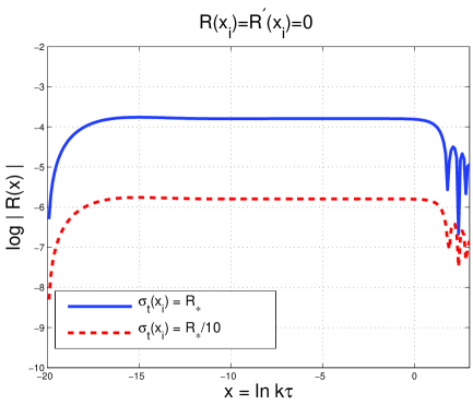
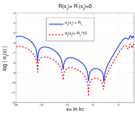
Figure 3: Illustrative examples where the initial conditions are dominated by the total anisotropic stress without leading to an early departure from the linear regime as suggested by Fig. 2.

6.4 The space of the initial Cauchy data

To solve the problem posed by Figs. 1, 2 and 3 it is interesting to derive more general criteria able to provide sufficient conditions for the avoidance of the sharp growth of the curvature perturbations when the Cauchy data are dominated by the anisotropic stress. The first step along this direction is to express Eqs. (6.1) and (6.2) in terms of an appropriately shifted variable defined as $w=(x-x_{i})$. The initial conditions at $x=x_{i}$ can then be translated into Cauchy data for $w=0$. In terms of $w$ Eqs. (6.1) and (6.2) can the be expressed as:

$$\frac{d^{3}\sigma_{\mathrm{t}}}{dw^{3}}-3\frac{d^{2}\sigma_{\mathrm{t}}}{dw^{2}}+\biggl{(}\frac{8}{5}R_{\nu}+2+\frac{6}{7}e^{2(w+x_{i})}\biggr{)}\frac{d\sigma_{\mathrm{t}}}{dw} = 16R_{\nu}\sigma_{\mathrm{t}}-\frac{48R_{\nu}}{5}\biggl{(}\frac{d{\mathcal{R}}}{dw}+\frac{{\mathcal{R}}}{9}e^{2(w+x_{i})}\biggr{)}$$ (6.8)

$$\frac{d^{2}{\mathcal{R}}}{dw^{2}}+\frac{d{\mathcal{R}}}{dw}+c_{\mathrm{st}}^{2}\,e^{2(w+x_{i})}{\mathcal{R}} = \biggl{(}\frac{d\sigma_{\mathrm{t}}}{dw}+2\sigma_{\mathrm{t}}\biggr{)}.$$ (6.9)

Taking now the Laplace transform of both sides of Eq. (6.1) we obtain the following difference equation:

$$g(s)s(s+1)-(s+2)f(s)-(1+s){\mathcal{R}}(0)+\sigma_{\mathrm{t}}(0)-{\mathcal{R}}^{\prime}(0)+c_{\mathrm{st}}^{2}e^{2x_{i}}g(s-2)=0,$$ (6.10)

where $g(s)$ and $f(s)$ are, respectively, the Laplace transforms of ${\mathcal{R}}(w)$ and of $\sigma_{\mathrm{t}}(w)$. Taking then the Laplace transform of both sides of Eq. (6.9), the following equation is obtained:

$$[8R_{\nu}(s-10)+5s(s-1)(s-2)]\,f(s)+48R_{\nu}\,s\,g(s)-48R_{\nu}{\mathcal{R}}(0)$$

$$-[10+8R_{\nu}+5s(s-3)]\sigma_{\mathrm{t}}(0)-5(s-3)\sigma_{\mathrm{t}}^{\prime}(0)-5\sigma_{\mathrm{t}}^{\prime\prime}(0)+$$

$$10e^{2x_{i}}\biggl{\{}\frac{3}{7}[(s-2)f(s-2)-\sigma_{\mathrm{t}}(0)]+\frac{8}{15}R_{\nu}g(s-2)\biggr{\}}=0.$$ (6.11)

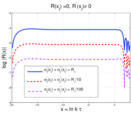
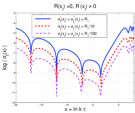
Figure 4: Examples of Cauchy data dominated by the anisotropic stress where initially ${\mathcal{R}}(x_{i})\neq{\mathcal{R}}^{\prime}(x_{i})$. The initial conditions are fixed in compliance with Eqs. (6.25).

Equations (6.10) and (6.11) form a system of difference equations that can be solved iteratively by neglecting, in the first approximation, the terms containing $\exp{(2x_{i})}$. As already mentioned earlier on in this section, $x_{i}=\ln{(k\tau_{i})}$ is relatively large and negative for the physical set of initial conditions. Typically $x_{i}\simeq{\mathcal{O}}(-20)$. Equation (6.10) can thus be written as:

$$g(s)s(s+1)-(s+2)f(s)=(1+s){\mathcal{R}}(0)-\sigma_{\mathrm{t}}(0)+{\mathcal{R}}^{\prime}(0),$$ (6.12)

while, under the same approximation, Eq. (6.11) becomes:

$$48R_{\nu}\,s\,g(s) + [8R_{\nu}(s-10)+5s(s-1)(s-2)]f(s)=48R_{\nu}{\mathcal{R}}(0)$$ (6.13)

$$+ [10+8R_{\nu}+5s(s-3)]\sigma_{\mathrm{t}}(0)+5(s-3)\sigma_{\mathrm{t}}^{\prime}(0)+5\sigma_{\mathrm{t}}^{\prime\prime}(0).$$

The explicit solution of Eqs. (6.12) and (6.13) is

$$g(s) = a_{1}(s){\mathcal{R}}(0)+a_{2}(s){\mathcal{R}}^{\prime}(0)+a_{3}(s)\sigma_{\mathrm{t}}(0)+a_{4}(s)\sigma_{\mathrm{t}}^{\prime}(0)+a_{5}(s)\sigma_{\mathrm{t}}^{\prime\prime}(0),$$ (6.14)

$$f(s) = b_{1}(s)\sigma_{\mathrm{t}}(0)+b_{2}(s)\sigma_{\mathrm{t}}^{\prime}(0)+b_{3}(s)\sigma_{\mathrm{t}}^{\prime\prime}(0)+b_{4}(s){\mathcal{R}}^{\prime}(0).$$ (6.15)

The functions $a_{j}(s)$ (with $j=1,\,2,\,3,\,4,\,5$) multiplying the initial conditions in Eqs. (6.14) are given by:

$$a_{1}(s)=\frac{1}{s},\qquad a_{2}(s)=\frac{4[8R_{\nu}\,(s-10)+5s(s-1)(s-2)]}{5\,s\,(s-1)\,(s-2)[(2s+1)^{2}+\beta^{2}]},$$

$$a_{3}(s)=\frac{4[96R_{\nu}+10(s-1)(s-2)]}{5\,s\,(s-1)\,(s-2)[(2s+1)^{2}+\beta^{2}]},$$

$$a_{4}(s)=\frac{4(s+2)(s-3)}{s(s-1)(s-2)[(2s+1)^{2}+\beta^{2}]},$$

$$a_{5}(s)=\frac{4(s+2)}{s(s-1)(s-2)[(2s+1)^{2}+\beta^{2}]},$$ (6.16)

where we introduced the auxiliary quantity $\beta(R_{\nu})=\sqrt{32R_{\nu}/5-1}$; With the same notations the functions $b_{i}(s)$ (with $i=1,\,2,\,3,\,4$) appearing in Eq. (6.15) are instead given by:

$$b_{1}(s)=\frac{4[5(s+1)(s-1)(s-2)+8R_{\nu}(s+7)]}{5(s-1)(s-2)[(2s+1)^{2}+\beta^{2}]},$$

$$b_{2}(s)=\frac{4(s+1)(s-3)}{(s-1)(s-2)[(2s+1)^{2}+\beta^{2}]},$$

$$b_{3}(s)=\frac{4(s+1)}{(s-1)(s-2)[(2s+1)^{2}+\beta^{2}]},$$

$$b_{4}(s)=-\frac{192\,R_{\nu}}{5(s-1)(s-2)[(2s+1)^{2}+\beta^{2}]}.$$ (6.17)

We can finally take the inverse transform of Eqs. (6.14) and (6.15) and go back either to the $w$ variable or to the $x$ variable. Except $a_{1}(s)$ (whose antitransform is constant in $w$-space), the structure of the poles of Eqs. (6.16) and (6.17) implies that each of the $a_{j}(s)$ and $b_{i}(s)$ leads, generally speaking, to three qualitatively different contributions:

• two exponential contributions increasing, respectively, as $e^{2w}$ and as $e^{w}$: these are the most dangerous terms that may take the curvature perturbations far from the linear regime at early time;

• a constant contribution possibly depending on $R_{\nu}$;

• an exponentially suppressed contribution going as $e^{-w/2}$; this contribution is modulated by linear combinations oscillating factors going proportional to $\cos{(\beta w/2)}$ and to $\sin{(\beta w/2)}$.

For instance the anti-transform of $a_{2}(s)$ can be written, in $w$-space as:

$${\mathcal{L}}^{-1}[a_{2}(s)] = -\frac{128R_{\nu}}{5(25+\beta^{2})}e^{2w}+\frac{288R_{\nu}}{5(9+\beta^{2})}e^{w}-\frac{32R_{\nu}}{1+\beta^{2}}+e^{-w/2}j(w,\beta),$$

$$j(w,\beta) = \frac{768\left(\beta^{2}-39\right)R_{\nu}}{5\beta\left(\beta^{2}+1\right)\left(\beta^{2}+9\right)\left(\beta^{2}+25\right)}\,\cos{(\beta w/2})$$

$$+ 2\biggl{[}\frac{1}{\beta}-\frac{32\left(\beta^{4}+166\beta^{2}-315\right)R_{\nu}}{5\beta\left(\beta^{2}+1\right)\left(\beta^{2}+9\right)\left(\beta^{2}+25\right)}\biggr{]}\sin{(\beta w/2)}.$$

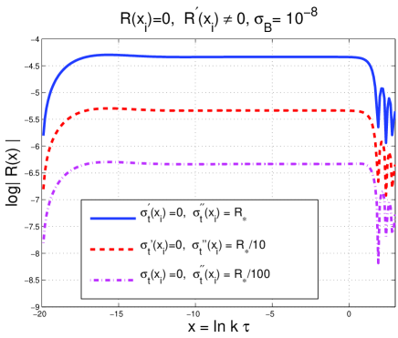
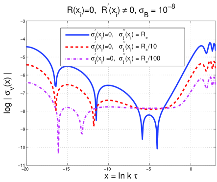
Figure 5: Illustrative examples of asymmetric initial conditions where $\sigma_{\mathrm{t}}(x_{i})\neq 0$ and $\sigma_{\mathrm{t}}^{\prime}(x_{i})\neq\sigma_{\mathrm{t}}^{\prime\prime}(x_{i})$. As in Fig. 4 the Cauchy data are fixed according to Eqs. (6.25).

Being exponentially suppressed, the oscillating contribution is immaterial for our discussion. Consequently the inverse Laplace transform of Eqs. (6.14) and (6.15) gives, in the $x$-parametrization:

$${\mathcal{R}}(x) = {\mathcal{R}}_{*}+\biggl{[}-\frac{16R_{\nu}}{15+4R_{\nu}}e^{2(x-x_{i})}+\frac{36R_{\nu}}{5+4R_{\nu}}e^{(x-x_{i})}\biggr{]}{\mathcal{R}}^{\prime}(x_{i})$$ (6.18)

$$+ \biggl{[}\frac{24R_{\nu}}{15+4R_{\nu}}e^{2(x-x_{i})}-\frac{48R_{\nu}}{5+4R_{\nu}}e^{(x-x_{i})}\biggr{]}\sigma_{\mathrm{t}}(x_{i})$$

$$+ \biggl{[}-\frac{5}{15+4R_{\nu}}e^{2(x-x_{i})}+\frac{15}{5+4R_{\nu}}e^{(x-x_{i})}\biggr{]}\sigma_{\mathrm{t}}^{\prime}(x_{i})$$

$$+ \biggl{[}\frac{5}{15+4R_{\nu}}e^{2(x-x_{i})}-\frac{15}{2(5+4R_{\nu})}e^{(x-x_{i})}\biggr{]}\sigma_{\mathrm{t}}^{\prime\prime}(x_{i})+{\mathcal{O}}\biggl{(}e^{-(x-x_{i})/2}\biggr{)},$$

$$\sigma_{\mathrm{t}}(x) = \biggl{[}\frac{36R_{\nu}}{15+4R_{\nu}}e^{2(x-x_{i})}-\frac{32R_{\nu}}{5+4R_{\nu}}e^{(x-x_{i})}\biggr{]}\sigma_{\mathrm{t}}(x_{i})$$ (6.19)

$$+ \biggl{[}-\frac{15}{2(15+4R_{\nu})}e^{2(x-x_{i})}+\frac{10}{5+4R_{\nu}}e^{(x-x_{i})}\biggr{]}\sigma_{\mathrm{t}}^{\prime}(x_{i})$$

$$+ \biggl{[}\frac{15}{2(15+4R_{\nu})}e^{2(x-x_{i})}-\frac{5}{5+4R_{\nu}}e^{(x-x_{i})}\biggr{]}\sigma_{\mathrm{t}}^{\prime\prime}(x_{i})$$

$$+ \biggl{[}-\frac{24R_{\nu}}{(15+4R_{\nu})}e^{2(x-x_{i})}+\frac{24R_{\nu}}{5+4R_{\nu}}e^{(x-x_{i})}\biggr{]}{\mathcal{R}}^{\prime}(x_{i})+{\mathcal{O}}\biggl{(}e^{-(x-x_{i})/2}\biggr{)}.$$

6.5 Taming the early departures from the linear regime

The presence (or the absence) of the diverging contributions in Eqs. (6.18) and (6.19) depends upon the Cauchy data. The exponentially increasing terms disappear from Eqs. (6.18) and (6.19) provided a pair of specific relations connects ${\mathcal{R}}^{\prime}(x_{i})$ and $\sigma_{t}(x_{i})$ to $\sigma_{\mathrm{t}}^{\prime}(x_{i})$ and $\sigma_{\mathrm{t}}^{\prime\prime}(x_{i})$.

More precisely, by looking at the leading contributions of Eq. (6.18) we can demand that the coefficients of the exponentially increasing contributions vanish identically for the initial Cauchy data. This request leads to a pair of relations among the initial data:

$$8R_{\nu}[3\sigma_{\mathrm{t}}(x_{i})-2{\mathcal{R}}^{\prime}(x_{i})]-5[\sigma_{\mathrm{t}}^{\prime}(x_{i})-\sigma_{\mathrm{t}}^{\prime\prime}(x_{i})]=0,$$ (6.20)

$$24R_{\nu}[3{\mathcal{R}}^{\prime}(x_{i})-4\sigma_{\mathrm{t}}(x_{i})]+15[2\sigma_{\mathrm{t}}^{\prime}(x_{i})-\sigma_{\mathrm{t}}^{\prime\prime}(x_{i})]=0.$$ (6.21)

The results of Eqs. (6.20) and (6.21) justify and explain the examples of Fig. 3: the initial conditions assigned in the numerical integration leading to Fig. 3 have been selected in such a way that Eqs. (6.20) and (6.21) are satisfied.

The same strategy can be used in Eq. (6.19) and we can demand that the coefficients of the exponentially increasing contributions vanish identically for the initial Cauchy data. The two supplementary relations obtained with this procedure are:

$$24R_{\nu}[3\sigma_{\mathrm{t}}(x_{i})-2{\mathcal{R}}^{\prime}(x_{i})]-15[\sigma_{\mathrm{t}}^{\prime}(x_{i})-\sigma_{\mathrm{t}}^{\prime\prime}(x_{i})]=0,$$ (6.22)

$$8R_{\nu}[3{\mathcal{R}}^{\prime}(x_{i})-4\sigma_{\mathrm{t}}(x_{i})]+5[2\sigma_{\mathrm{t}}^{\prime}(x_{i})-\sigma_{\mathrm{t}}^{\prime\prime}(x_{i})]=0.$$ (6.23)

The system formed by Eqs. (6.20)–(6.21) is not linearly independent from the system of Eqs. (6.22)–(6.23): if we multiply by a factor of $3$ Eq. (6.20) we obtain Eq. (6.22) and if we multiply by a factor of $3$ Eq. (6.23) we obtain Eq. (6.21). Thus, if Eqs. (6.20) and (6.21) are satisfied also Eqs. (6.22)–(6.23) will also be satisfied.

Equations (6.20)–(6.21) can be solved by relating the derivatives of the anisotropic stress to $\sigma_{\mathrm{t}}(x_{i})$ and to ${\mathcal{R}}^{\prime}(x_{i})$:

$$\sigma_{\mathrm{t}}^{\prime}(x_{i})=-\frac{8}{5}R_{\nu}[{\mathcal{R}}^{\prime}(x_{i})-\sigma_{\mathrm{t}}(x_{i})],\qquad\sigma_{t}^{\prime\prime}(x_{i})=\frac{8}{5}R_{\nu}[{\mathcal{R}}^{\prime}(x_{i})-2\sigma_{\mathrm{t}}(x_{i})].$$ (6.24)

Equation (6.24) provides a quantitative solution to the problem posed by Figs. 2 and 3. The first and second derivatives of the anisotropic stress must be tuned in order to tame the exponential growth of the curvature perturbations for a generic initial value of ${\mathcal{R}}^{\prime}$ and $\sigma_{t}$. The inverse viewpoint can be adopted by using $\sigma_{\mathrm{t}}^{\prime}(x_{i})$ and $\sigma_{\mathrm{t}}^{\prime\prime}(x_{i})$ as pivotal variables. Indeed, inverting Eq. (6.24) we will have:

$${\mathcal{R}}^{\prime}(x_{i})=-\frac{5}{8R_{\nu}}[2\sigma_{\mathrm{t}}^{\prime}(x_{i})+\sigma_{\mathrm{t}}^{\prime\prime}(x_{i})],\qquad\sigma_{\mathrm{t}}(x_{i})=-\frac{5}{8R_{\nu}}[\sigma_{\mathrm{t}}^{\prime}(x_{i})+\sigma_{\mathrm{t}}^{\prime\prime}(x_{i})].$$ (6.25)

The criteria given by Eq. (6.24) (or equivalently by Eq. (6.25)) have been obtained after various steps involving some plausible approximations. It is therefore interesting to present direct numerical tests of these criteria. The illustrative examples of Figs. 4, 5 and 6 confirm the heuristic validity of the relations (6.24) and (6.25).

In Fig. 4 we explore a set of initial data dominated by the anisotropic stress but different from the initial conditions leading to Fig. 3. While ${\mathcal{R}}(x_{i})={\mathcal{R}}^{\prime}(x_{i})=0$ in Fig. 3, in Fig. 4 ${\mathcal{R}}(x_{i})=0$ and ${\mathcal{R}}^{\prime}(x_{i})\neq 0$. The values of ${\mathcal{R}}^{\prime}(x_{i})$ and of $\sigma_{\mathrm{t}}(x_{i})$ are fixed, in terms of $\sigma_{\mathrm{t}}^{\prime}(x_{i})$ and of $\sigma_{\mathrm{t}}^{\prime\prime}(x_{i})$ by Eq. (6.25). In the legend of Fig. 4 the initial values of $\sigma_{\mathrm{t}}^{\prime}(x)$ and of $\sigma_{\mathrm{t}}^{\prime\prime}(x)$ are explicitly mentioned. As implied by the criteria leading to Eq. (6.25) we do expect the absence of diverging contributions of the type of Fig. 2. This is exactly what happens. Notice that none of the fluctuations illustrated in Fig. 4 become nonlinear while the relevant wavelengths are still larger than the Hubble radius.

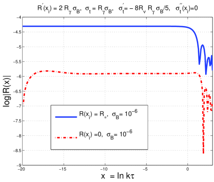
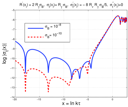
Figure 6: The numerical integration corresponding to the Cauchy data of Eqs. (6.26) and (6.27). As in Figs. 4 and 5 the Cauchy data are fixed according to Eqs. (6.25).

In Fig. 5 we explore yet a different set of initial conditions that are asymmetric both in the curvature and in the anisotropic stress. In the left panel we illustrate, as usual, the evolution of the curvature perturbations for different values of $\sigma_{\mathrm{t}}^{\prime\prime}(x_{i})$ (expressed in units of ${\mathcal{R}}_{*}$). In the right panel of Fig. 5 we illustrate directly the anisotropic stress of the neutrinos (instead of the total anisotropic stress containing also the magnetic contribution). As in the case of Fig. 4 the values of ${\mathcal{R}}^{\prime}(x_{i})$ and of $\sigma_{\mathrm{t}}(x_{i})$ are fixed, in terms of $\sigma_{\mathrm{t}}^{\prime}(x_{i})$ and of $\sigma_{\mathrm{t}}^{\prime\prime}(x_{i})$ by Eq. (6.25). Also in Fig. 5 the criteria expressed by Eqs. (6.24) and (6.25) are clearly verified.

As a last example let us consider the results of Fig. 6. If for $x=x_{i}$ the only contribution to the total anisotropic stress is given only by the magnetic term, then $\sigma_{\mathrm{t}}=R_{\gamma}\sigma_{B}$ but $\sigma_{\nu}(x_{i})=0$. Recalling the solution obtained in Eq. (5.19) we shall have that ${\mathcal{R}}(x)={\mathcal{R}}_{*}+2R_{\gamma}\sigma_{B}(x-x_{i})$, implying that

$${\mathcal{R}}(x_{i})={\mathcal{R}}_{*},\qquad{\mathcal{R}}^{\prime}(x_{i})=2R_{\gamma}\sigma_{B}.$$ (6.26)

The fate of these initial data can be investigated using the results developed so far. The previous analysis tells that if $\sigma_{\mathrm{t}}^{\prime}(x_{i})$ and $\sigma_{\mathrm{t}}^{\prime\prime}(x_{i})$ are assigned arbitrarily, the curvature perturbations will become eventually nonlinear unless

$$\sigma_{\mathrm{t}}^{\prime}(x_{i})=-\frac{8}{5}R_{\nu}R_{\gamma}\sigma_{B},\qquad\sigma_{\mathrm{t}}^{\prime\prime}(x_{i})=0.$$ (6.27)

The initial conditions of Eqs. (6.26) and (6.27) are located within the tuning volume of the initial Cauchy data satisfying Eqs. (6.20) and (6.21). Equation (6.27) fixes the first and second derivatives of the total anisotropic stress which are not specified even if we already required $\sigma_{\nu}(x_{i})=0$. Only if the Cauchy data satisfy Eq. (6.27) we can safely argue that the exponentially increasing contributions are tamed.

The initial conditions of Eqs. (6.26)–(6.27) can be tested by direct numerical integration. The results are illustrated in Fig. 6 and, once more, the criteria derived from Eqs. (6.20) and (6.21) are confirmed. In the left panel of Fig. 6 we compare the case ${\mathcal{R}}(x_{i})={\mathcal{R}}_{*}$ (full line) and the case ${\mathcal{R}}(x_{i})=0$ (dot-dashed line). In the right panel we illustrate the total anisotropic stress. As expected on the basis of the more general considerations discussed before, both the curvature perturbations and the total anisotropic stress do not exhibit exponentially divergent contributions that will be however present if $\sigma_{\mathrm{t}}^{\prime}(x_{i})$ and $\sigma_{\mathrm{t}}^{\prime\prime}(x_{i})$ would be arbitrarily assigned as previously illustrated in Fig. 2. We can thus conclude that the heuristic criteria expressed by Eqs. (6.24) and (6.25) are confirmed by the diverse numerical examples.

In summary, the problem of initial data of the large-scale curvature perturbations has been reduced to an ordinary Cauchy problem fully determined by five initial data: two involving the curvature perturbations and three involving the total anisotropic stress. The absence of exponentially increasing terms reduces the five-dimensional space to a three-dimensional Cauchy volume where the initial data are related by two linearly independent relations. Our heuristic criteria have been derived by trying to formulate more faithfully a Cauchy problem for the large-scale curvature perturbations. The derived relations seem to solve a more general boundary value problem insofar as they give a sufficient condition for the constancy of the curvature perturbations even when the large-scale initial conditions are dominated by the anisotropic stress.

7 Concluding remarks

We demonstrated that two coupled differential equations of second and third order describe, respectively, the evolution of the quasinormal mode of the plasma and of the anisotropic stress. The total anisotropic stress, the non-adiabatic pressure fluctuations and the large-scale magnetic fields are present on equal footing as potential sources of inhomogeneities. On the basis of the reported results, the proposed approach seems reasonably simple and direct.

When all the supplementary sources of inhomogeneity vanish, the quasinormal modes of the plasma describe the phonons of a gravitating fluid in a conformally flat background geometry firstly derived by Lukash in the early eighties. The obtained system is gauge-invariant. The derivation can be presented and interpreted both in the conformally Newtonian and in the synchronous coordinate systems. Various physical solutions have been obtained with particular attention to the standard concordance paradigm and to its magnetized completion. After solving for the quasi normal mode and for the anisotropic stress, all the scalar fluctuations of the plasma can be easily deduced without the addition of further assumptions.

The large-scale symmetries of the system suggest that Cauchy data of large-scale curvature perturbations can be reduced to an initial value problem involving the quasinormal mode, the total anisotropic stress and its first two derivatives with respect to an appropriately rescaled variable measuring the ratio between the particle horizon and the physical wavelength. As an illustrative example, a set of consistency conditions among the Cauchy data, guaranteeing the validity of the perturbative expansion for generic anisotropic stresses, has been analytically deduced and numerically tested.

References

- [1] Ya. B. Zeldovich, A. A. Ruzmaikin, and D.D. Sokoloff, Magnetic Fields in Astrophysics (Gordon and Breach Science, New York, 1983).
- [2] K. Enqvist, Int. J. Mod. Phys. D 7, 331 (1998); M. Giovannini, Int. J. Mod. Phys. D 13, 391 (2004); Class. Quant. Grav. 23, R1 (2006).
- [3] V. N. Lukash, Sov. Phys. JETP 52, 807 (1980) [Zh. Eksp. Teor. Fiz. 79, 1601 (1980)].
- [4] V. N. Lukash and I. D. Novikov, Lectures on the very early universe in Observational and Physical Cosmology, II Canary Islands Winter School of Astrophysics, eds. F. Sanchez, M. Collados and R. Rebolo (Cambridge University Press, Cambridge UK, 1992), p. 3; V. Strokov, Astron. Rep. 51, 431 (2007).
- [5] E. M. Lifshitz Zh. Eksp. Teor. Fiz. 16, 587 (1946) [J. Phys. (USSR) 10, 116 (1946)]; E. M. Lifshitz and I. M. Khalatnikov, Adv. Phys. 12, 185 (1963).
- [6] E. M. Lifshitz and I. M. Khalatnikov, Adv. Phys. 12, 185 (1963); E. M. Lifshitz Zh. Eksp. Teor. Fiz. 16, 587 (1946).
- [7] J. Bardeen, Phys. Rev. D22, 1882 (1980).
- [8] H. Kodama, M. Sasaki, Prog. Theor. Phys. Suppl. 78, 1 (1984); M. Sasaki, Prog. Teor. Phys. 76, 1036 (1986).
- [9] G. V. Chibisov, V. F. Mukhanov, Mon. Not. Roy. Astron. Soc. 200, 535 (1982); V. F. Mukhanov, Sov. Phys. JETP 67, 1297 (1988) [Zh. Eksp. Teor. Fiz. 94, 1 (1988)].
- [10] R. H. Brandenberger, R. Kahn and W. H. Press, Phys. Rev. D 28, 1809 (1983); R. H. Brandenberger and R. Kahn, Phys. Rev. D 29, 2172 (1984).
- [11] J. Bardeen, P. Steinhardt, and M. Turner, Phys. Rev. D28, 679 (1983); J. A. Frieman and M. S. Turner, Phys. Rev. D 30, 265 (1984).
- [12] J -c. Hwang, Astrophys. J. 375, 443 (1990); Class. Quant. Grav. 11, 2305 (1994).
- [13] J. -c. Hwang and H. Noh, Phys. Lett. B 495, 277 (2000); Phys. Rev. D 65, 124010 (2002).
- [14] J. -C. Hwang and H. Noh, Class. Quant. Grav. 19, 527 (2002); Phys. Rev. D 73, 044021 (2006); H. S. Kim, J. -c. Hwang, Phys. Rev. D 74, 043501 (2007).
- [15] K. Enqvist, H. Kurki-Suonio and J. Valiviita, Phys. Rev. D 62, 103003 (2000); J. Valiviita and V. Muhonen, Phys. Rev. Lett. 91, 131302 (2003).
- [16] H. Kurki-Suonio, V. Muhonen and J. Valiviita, Phys. Rev. D 71, 063005 (2005); R. Keskitalo, H. Kurki-Suonio, V. Muhonen and J. Valiviita, JCAP 0709, 008 (2007).
- [17] M. Giovannini, Phys. Rev. D 70, 123507 (2004); Phys. Rev. D 73, 101302 (2006).
- [18] M. Giovannini, Phys. Rev. D 74, 063002 (2006); Class. Quant. Grav. 23, 4991 (2006); PMC Phys. A 1, 5 (2007); M. Giovannini and K. E. Kunze, Phys. Rev. D 77, 063003 (2008); Phys. Rev. D 77, 061301 (2008); M. Giovannini, Phys. Rev. D 79, 103007 (2009); Phys. Rev. D 79, 121302 (2009).
- [19] D. G. Yamazaki, K. Ichiki, K. -i. Umezu and H. Hanayama, Phys. Rev. D 74, 123518 (2006); T. Kahniashvili and B. Ratra, Phys. Rev. D 75, 023002 (2007); F. Finelli, F. Paci and D. Paoletti, Phys. Rev. D 78, 023510 (2008).
- [20] K. Kojima, T. Kajino and G. J. Mathews, JCAP 1002, 018 (2010); M. Giovannini, Class. Quant. Grav. 27, 105011 (2010); J. R. Shaw and A. Lewis, Phys. Rev. D 81, 043517 (2010); P. Trivedi, K. Subramanian and T. R. Seshadri, Phys. Rev. D 82, 123006 (2010); M. Giovannini, Phys. Rev. D 81, 123003 (2010).
- [21] D. F. Mota, J. R. Kristiansen, T. Koivisto and N. E. Groeneboom, Mon. Not. Roy. Astron. Soc. 382, 793 (2007); W. Hu, Astrophys. J. 506, 485 (1998).
- [22] S. Weinberg, Cosmology (Oxford University Press, Oxford 2008).
- [23] M. Giovannini, A Primer on the Physics of the Cosmic Microwave Background (World Scientific, Singapore 2008).
- [24] P. Naselsky and I. Novikov, Astrophys. J. 413, 14 (1993); H. Jorgensen, E. Kotok, P. Naselsky, and I. Novikov, Astron. Astrophys. 294, 639 (1995); U. Seljak, Astrophys. J. 435, L87 (1994); C. P. Ma and E. Bertschinger, Astrophys. J. 455, 7 (1995).
- [25] P. J. E. Peebles and J. T. Yu, Astrophys. J. 162 815 (1970); P. J. E. Peebles, Astrophys. J. 263, L1 (1982).
- [26] W. Press and E. Vishniac, Astrophys. J. 239, 1 (1980); Astrophys. J. 236, 323 (1980).
- [27] S. Weinberg, Phys. Rev. D 67, 123504 (2003); Phys. Rev. D 69, 023503 (2004).
- [28] D. N. Spergel et al., 148, 175 (2003); D. N. Spergel et al., ibid. 170, 377 (2007); L. Page et al. Astrophys. J. Suppl. 170, 335 (2007).
- [29] B. Gold et al., Astrophys. J. Suppl. 192, 15 (2011); D. Larson, et al., ibid. 192, 16 (2011); C. L. Bennett et al., ibid. 192, 17 (2011); G. Hinshaw et al., ibid. 208 19 (2013); C. L. Bennett et al., ibid. 208 20 (2013).
- [30] P. A. R. Ade et al. [BICEP2 Collaboration], Phys. Rev. Lett. 112, 241101 (2014).