Stress-Minimizing Orthogonal Layout
of Data Flow Diagrams with Ports

Abstract

We present a fundamentally different approach to orthogonal layout of data flow diagrams with ports. This is based on extending constrained stress majorization to cater for ports and flow layout. Because we are minimizing stress we are able to better display global structure, as measured by several criteria such as stress, edge-length variance, and aspect ratio. Compared to the layered approach, our layouts tend to exhibit symmetries, and eliminate inter-layer whitespace, making the diagrams more compact. ctor models, data flow diagrams, orthogonal routing, layered layout, stress majorization, force-directed layout

Sect. 1 Introduction

Actor-oriented data flow diagrams are commonly used to model movement of data between components in complex hardware and software systems [13]. They are provided in many widely used modelling tools including LabVIEW (National Instruments Corporation), Simulink (The MathWorks, Inc.), EHANDBOOK (ETAS), SCADE (Esterel Technologies), and Ptolemy (UC Berkeley). Complex systems are modelled graphically by composing actors, i. e., reusable block diagrams representing well-defined pieces of functionality. Actors can be nested—i. e., composed of other actors—or atomic. Fig. 1a shows an example of a data flow diagram with four nested actors. Data flow is shown by directed edges from the source port where the data is constructed to the target port where the data is consumed. By convention the edges are drawn orthogonally and the ports are fixed in position on the actors’ boundaries. Automatic layout of data flow diagrams is important: Klauske and Dziobek [12] found that without automatic layout about 30 % of a modeller’s time is spent manually arranging elements.

Current approaches to automatic layout of data flow diagram are modifications of the well-known Sugiyama layer-based layout algorithm [17] extended to handle ports and orthogonal edges. In particular Schulze et al. [15] have spent many years developing specialised layout algorithms that are used, for instance, in the EHANDBOOK and Ptolemy tools. However, their approach has a number of drawbacks. First, it employs a strict layering which may result in layouts with poor aspect ratio and poor compactness, especially when large nodes are present. Furthermore, the diagrams often have long edges and the underlying structure and symmetries may not be revealed. A second problem with the approach of Schulze et al. is that it uses a recursive bottom-up strategy to compute a layout for nested actors independent of the context in which they appear.

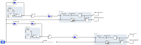
(a) Layout with layer-based algorithm KLay Layered by Schulze et al.

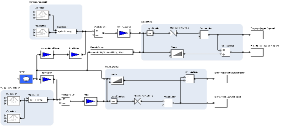
(b) Layout with the CoDaFlow algorithm presented here.

Figure 1: Two layouts of the same diagram. The result of our method, shown in (b), has less stress, lower edge length variance, less area, and better aspect ratio.

This paper presents a fundamentally different approach to the layout of actor-oriented data flow diagrams designed to overcome these problems. A comparison of our new approach with standard layer-based algorithm KLay Layered is shown in Fig. 1. Our starting point is constrained stress majorization [3]. Minimizing stress has been shown to improve readability by giving a better understanding of important graph structure such as cliques, chains and cut nodes [4]. However, stress-minimization typically results in a quite “organic” look with nodes placed freely in the plane that is quite different to the very “schematic” arrangement involving orthogonal edges, a left-to-right “flow” of directed edges, and precise alignment of node ports that practitioners prefer.

The main technical contribution of this paper is to extend constrained stress majorization to handle the layout conventions of data flow diagrams. In particular we: (1) augment the $P$-stress [7] model to handle ports that are constrained to node boundaries but are either allowed to float subject to ordering constraints or else are fixed to a given node boundary side, and (2) extend Adaptive Constrained Alignment (ACA) [10] for achieving grid-like layout to handle directed edges, orthogonal routing, ports, and widely varying node dimensions.

An empirical evaluation of the new approach (Sect. 4) shows it produces layouts of comparable quality to the method of Schulze et al. but with a different trade off between aesthetic criteria. The layouts have more uniform edge length, better aspect ratio, and are more compact but have slightly more edge crossings and bends. Furthermore, our method is more flexible and requires far less implementation effort. The Schulze et al. approach took a team of developers and researchers several years to implement by extensively augmenting the Sugiyama method. While their infrastructure allows a flexible configuration of the existing functionality [15], it is very restrictive and brittle when it comes to extensions that affect multiple phases of the algorithm. The method described in this paper took about two months to implement and is also more extendible since it is built on modular components with well-defined work flows and no dependencies on each other.

Related Work.

The most closely related work is the series of papers by Schulze et al. that show how to extend the layer-based approach to handle the layout requirements of data flow diagrams [15, 16]. Their work presents several improvements over previous methods to reduce edge bend points and crossings in the presence of ports. While the five main phases (classically three) of the layer-based approach are already complex, they introduce between 10 and 20 intermediate processes in order to address additional requirements. The authors admit that their approach faces problems with unnecessary crossings of inter-hierarchy edges as they layout compound graphs bottom-up, i. e., processing the most nested actor diagrams first. Related work in the context of the layer-based approach has been studied thoroughly in [15, 16]. Chimani et al. present methods to consider ports and their constraints during crossing minimization within the upward planarization approach [2]. While the number of crossings is significantly reduced, the approach eventually induces a layering, suffering from the same issues as above. There is no evaluation with real-world examples. Techniques from the area of VLSI design and other approaches that specifically target compound graphs have been discussed before and found to be insufficient to fulfil the layout requirements for data flow diagrams [16], especially due to lacking support for different port constraints.

Sect. 2 CoDaFlow — The Algorithm

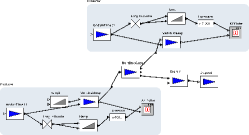
(a) After Node Positioning

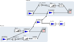
(b) After Node Alignment

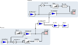
(c) After Edge Routing

Figure 2: The results of pipeline stages (1), (2), (3) are shown in (a), (b), (c), respectively.

Data flow diagrams can be modelled as directed graphs $G=(V,E,P,\pi)$ where nodes or vertices $v\in V$ are connected by edges $e\in E\subseteq P\times P$ through ports $p\in P$—certain positions on a node’s perimeter—and $\pi:P\rightarrow V$ maps each port $p$ to the parent node $\pi(p)$ to which it belongs. An edge $e=(p_{1},p_{2})$ is directed, outgoing from port $p_{1}$ and incoming to $p_{2}$. A hyperedge is a set of edges where every pair of edges shares a common port.

To better show flow it is preferable for sources of edges to be to the left of their targets and by convention edges are routed in an orthogonal fashion. Ports can—depending on the application—be restricted by certain constraints, e. g., all ports with incoming edges should be placed on the left border of the node. Spönemann et al. define five types of port constraints [16], ranging from ports being free to float arbitrarily on a node’s perimeter, to ports having well-defined positions relative to nodes. Nodes that contain nested diagrams, i. e., child nodes, are referred to as compound nodes (as opposed to atomic nodes); a graph that contains compound nodes is a compound graph. We refer to the ports of a compound node as hierarchical ports. These can be used to connect atomic nodes inside a compound node to atomic nodes on the outside.

The main additional requirements for layout of data flow diagrams on top of standard graph drawing conventions are therefore [16]: (R1) clearly visible flow, (R2) ports and port constraints, (R3) compound nodes, (R4) hierarchical ports, (R5) orthogonal edge routing, and (R6) orthogonalized node positions to emphasize R1 using horizontal edges.

The starting point for our approach is constrained stress majorization [3]. This extends the original stress majorization model [9] to support separation constraints that can be used to declaratively enforce node alignment, non-overlap of nodes, flow in directed graphs, and to cluster nodes inside non-overlapping regions. Brandes et al. [1] provide one method to orthogonalise an existing layout based on the topology-shape-metrics approach, but in order to handle requirements R1–6 we instead use the heuristic approach of Kieffer et al. [10] to apply alignment constraints within the stress-based model.

Our Constrained Data Flow (CoDaFlow) layout algorithm is a pipeline with three stages:

1. Constrained Stress-Minimizing Node Positioning

2. Grid-Like Node Alignment

3. Orthogonal Edge Routing

The intermediate results of this pipeline are depicted in Fig. 2. Single stages can be omitted, e. g., when no edge routing is required or initial node positions are given. In this section we restrict our attention to flat graphs, i. e., those without compound nodes, while Sect. 3 extends the ideas to compound graphs.

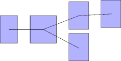
(a)

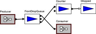
(b)

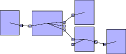
(c)

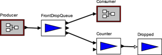
(d)

Figure 3: Awareness of ports is important to achieve good node positioning. (a) and (c) show internal representations of what is passed to the layout algorithm, (b) and (c) show the resulting drawings. (a) is unaware of ports and yields node positions that introduce an edge crossing in (b). In (c) ports are considered and the unnecessary crossing is avoided in (d). Note, however, while the chance is higher that (c) is cross free, it is not guaranteed.

2.1 Constrained Stress-Minimizing Node Positioning

Traditional stress models for graph layout expect a simple graph without ports, so a key idea in order to handle data flow diagrams is to create a small node to represent each port, called a port node or port dummy, as in Fig. 3c. If $D$ is the set of all these, and $\delta:P\rightarrow D$ maps each port to the dummy node that represents it, we construct a new graph $G^{\prime}=(V^{\prime},E^{\prime})$ where $V^{\prime}=V\cup D$, and

$$E^{\prime}=\{(\delta(p_{1}),\delta(p_{2})):(p_{1},p_{2})\in E\}\cup\{(\pi(p),\delta(p)):p\in P\}$$

includes one edge representing each edge of the original graph, and an edge connecting each port dummy to its parent node. We refer to the $v\in V$ as proper nodes.

Depending on the specified port constraints (R2) we restrict the position of each port dummy $\delta(p)$ relative to its parent node $\pi(p)$ using separation constraints. For instance, for a rigid relative position we use one separation constraint in each dimension, whereas we retain only the $x$-constraint if $\delta(p)$ need only appear on the left or right side of $\pi(p)$. The use of port nodes allows the constrained stress-minimizing layout algorithm to untangle the graph while being aware of relative port positions, resulting in fewer crossings, as illustrated in Fig. 3.

Our constrained stress-based layout uses the methods of Dwyer et al. [3] to minimize the P-stress function [7], a variant of stress [9] that does not penalise unconnected nodes being more than their desired distance apart:

$$\sum_{u<v\in V^{\prime}}w_{uv}\left(\left(\ell p_{uv}-b(u,v)\right)^{+}\right)^{2}+\sum_{(u,v)\in E^{\prime}}\ell^{-2}\left(\left(b(u,v)-\ell\right)^{+}\right)^{2}$$ (1)

where $b(u,v)$ is the Euclidean distance between the boundaries of nodes $u$ and $v$ along the straight line connecting their centres, $p_{uv}$ the number of edges on the shortest path between nodes $u$ and $v$, $\ell$ an ideal edge length, $w_{uv}=(\ell p_{uv})^{-2}$, and $(z)^{+}=\max(z,0)$.

Ideal Edge Lengths.

Instead of using a single ideal edge length $\ell$ as in (1), which can result in cluttered areas where multiple nodes are highly connected, we may assign custom edge lengths $\ell_{uv}$, choosing larger values to separate such nodes. In Fig. 3 the ideal edge lengths of the two outgoing edges of the FrontDropQueue actor are chosen slightly larger than for the two other edges.

The length of the edge $(\pi(p),\delta(p))$ connecting a port dummy to its parent node is set to the exact distance from the node’s center to the port’s center.

Emphasizing Flow.

A common requirement for data flow diagrams is that the majority of edges point in the same direction (here left-to-right). For this we introduce separation constraints for edges ($u$, $v$) of the form $x_{u}+g\leq x_{v}$, where $g>0$ is a pre-defined spacing value, ensuring that $u$ is placed left of $v$. We refer to these constraints as flow constraints.

Special care has to be taken for cycles, as they would introduce contradicting constraints. We experimented with different strategies to handle this. 1) We introduced the constraints even though they were contradicting (and let the solver choose which one(s) to reject); 2) We did not generate any flow constraints for edges that are part of a strongly connected component; 3) We employed a greedy heuristic by Eades et al. [8] (known from the layer-based approach) to find the minimal feedback arc set, and withheld flow constraints for the edges in this set. Our experiments showed that the third strategy yields the best results.

Execution.

We perform three consecutive layout runs, iteratively adding constraints: 1) Only port constraints are applied, allowing the graph to untangle and expose symmetry; 2) Flow constraints are added, but overlaps are still allowed so that nodes can float past each other, swapping positions where necessary; 3) Non-overlap constraints are applied to separate all nodes as desired.

2.2 Grid-like Node Alignment

While yielding a good distribution of nodes overall, stress-minimization tends to produce an organic layout with paths splayed at all angles, which is inappropriate for data flow diagrams. The layout needs to be orthogonalized, i. e., connected nodes brought into alignment with one another so that where possible edges form straight horizontal lines, visually emphasizing horizontal flow.

For this purpose we apply the Adaptive Constrained Alignment (ACA) algorithm [10]. Since it respects existing flow constraints, it only attempts to align edges horizontally. However, our replacement of the given graph $G$ by the auxiliary graph $G^{\prime}$ with port nodes tends to subvert the original intentions of ACA, so it requires some adaptation. Whereas the original ACA algorithm expected at most one proper node to be aligned with another in a given compass direction, in our case (with ports) it will often be desirable to have more. See Fig. 4.

In order to adapt ACA to the new port model we made it possible to ignore certain edges—namely those connecting port nodes to their parents—and also generalised its overlap prevention methods significantly. Instead of the simple procedure for preventing multiple alignments in a single compass direction [10], we use the VPSC solver [5] for trial satisfaction of existing constraints, the new potential alignment, as well as non-overlap constraints between all nodes and a dummy node representing the potentially aligned edge.

Thus, while the ACA process continues to merely centre-align nodes—in this case port nodes $d\in D$—we have allowed it to in effect align several proper nodes $v_{1},\ldots,v_{k}\in V$ with a single one $u\in V$ at port positions as in Fig. 4, meeting the requirement R6 of data flow diagrams.

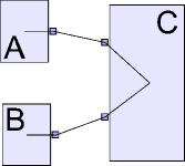
(a) Proper nodes connected via port nodes

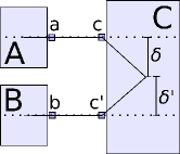
(b) Ports aligned by ACA

Figure 4: In the new port model, two proper nodes may be connected to the same side of another via ports, as in (a). The systematic use of offset alignments between port nodes and their parents, i. e., constraints of the form $y_{\delta(p)}+\delta=y_{\pi(p)}$, $\delta\neq 0$ as shown in (b), creates a risk of node-edge and node-node overlaps far exceeding what was anticipated with the original ACA algorithm, as could have occurred here had node $B$ been as tall as node $C$, for example. We have extended ACA to properly handle such cases.

2.3 Edge Routing

We now consider node positions to be fixed, and use the methods of Wybrow et al. [18] to route the edges orthogonally. We return from $G^{\prime}$ to $G$, using the final positions of the port nodes $d\in D$ to set routing pins, fixed port positions on the nodes $v\in V$ where the edges should connect.

Sect. 3 Handling Compound Graphs

When handling compound graphs, different strategies for dealing with compound nodes. Schulze et al. employ a bottom-up strategy, treating every compound node as a separate graph, starting with the inner-most nodes. This allows application of different layout algorithms to each subgraph which reduces the size of the layout problem, and possibly the overall execution time. They remark, however, that the procedure can yield unsatisfying layouts since the surroundings of a compound node are not known; see Fig. 5a for an example where two unnecessary crossings are created inside the TM controllers actor and two separate networks are interleaved. A global approach would solve this issue, positioning all compound nodes along with their children at the same time.

Even though we focus our attention on a global approach in what follows, our methods are flexible in that we may choose between a bottom-up and a global strategy in each stage of our pipeline.

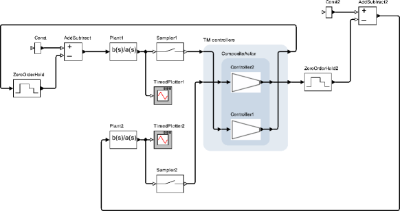
(a) Layout with layer-based methods by Schulze et al.

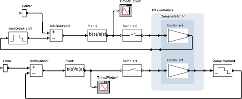
(b) Layout with the CoDaFlow algorithm presented here.

Figure 5: Two layouts of the same Ptolemy diagram. While two distinct networks are interleaved in (a), they are clearly separated and the two crossings are avoided in (b).

A compound graph $G$ is transformed into $G^{\prime}$ as above, which is used to construct a flat graph $G^{\prime\prime}=(A,E^{\prime\prime})$ where $A\subseteq V^{\prime}$ is the set of atomic nodes and their port nodes, and $E^{\prime\prime}=U\cup H$ with

$$U= \{(\delta(p_{1}),\delta(p_{n})):\pi(p_{1}),\pi(p_{n})\in A\}$$

$$H= \{(\delta(p_{1}),\delta(p_{n})):\exists(p_{1},p_{2}),(p_{2},p_{3}),\dots,(p_{n-2},p_{n-1}),(p_{n-1},p_{n})\in E:$$

$$\pi(p_{1}),\pi(p_{n})\in A\wedge\pi(p_{2}),\dots,\pi(p_{n-1})\in V\backslash A\}$$

Intuitively, compound nodes are neglected along with their ports and only atomic nodes are retained. Sequences of edges that span hierarchy boundaries, e. g., the three edges between Sampler2 and Controller2 in Fig. 5b, are replaced by a single edge that directly connects the two atomic nodes. Note that for hyperedges multiple edges have to be created. Cluster constraints guarantee that children of compound nodes are kept close together and are not interleaved with any other nodes. For instance, the CompositeActor in Fig. 5b yields a cluster containing Controller1 and Controller2.

To return to $G$, the clusters’ dimensions, i. e., their rectangular bounding boxes, are applied to the compound nodes in $V\backslash A$. The edges in $H$ are split into segments $s_{1},\dots,s_{n}$ based on the crossing points $c_{i}$ with clusters. The route of $s_{i}$ is applied to the corresponding edge $e\in E$ and the $c_{i}$ determine the positions of the hierarchical ports.

Sect. 4 Evaluation and Discussion

We evaluate our approach on a set of data flow diagrams that ship with the Ptolemy project, comparing with the KLay layered algorithm of Schulze et al. Diagrams were chosen to be roughly the size Klauske found to be typical for real-world Simulink models from the automotive industry [11] (about 20 nodes and 30 edges per hierarchy level).

Metrics.

Well established metrics to assess the quality of a drawing are edge crossings and edge bends [14], two metrics directly optimized by the layer-based approach. More recently, stress and edge length variance were found to have a significant impact on the readability of a drawing [4]. Additionally, we regard compactness in terms of aspect ratio and area.

So that comparisons of edge length and of layout area can be meaningful, we set the same value for KLay Layered’s inter-layer distance and CoDaFlow’s ideal separation between nodes.

The $P$-stress of a given (already layouted) diagram depends on the choice of the ideal edge length $\ell$ in (1), and the canonical choice $\bar{\ell}$ is that where the function takes its global minimum. If $L$ is a list of all the individual ideal lengths $\ell_{uv}=b(u,v)/p_{uv}$, then $\bar{\ell}$ is equal to the contraharmonic mean $C(L_{j})$ (i. e., the weighted arithmetic mean in which the weights equal the values) over a certain sublist $L_{j}\subseteq L$. Namely, if $L_{E}=\langle\ell_{uv}:(u,v)\in E\rangle$ and $L\setminus L_{E}=\langle\ell_{1}\leq\ell_{2}\leq\cdots\leq\ell_{\nu}\rangle$, then $L_{j}=L_{E}\cup\langle\ell_{1},\ell_{2},\ldots,\ell_{j}\rangle$ for some $0\leq j\leq\nu$. Since $\nu$ is finite, we can compute each $C(L_{j})$ and take $\bar{\ell}$ to be that at which the $P$-stress is minimized. See Appendix 0.B.

Table 1: Evaluations of 110 flat diagrams with 10–23 nodes (9–30 edges) and 10 compound diagrams with 12–38 nodes (12–52 edges). Figures for stress, average edge length, variance in edge length, and area are given as the ratio of CoDaFlow divided by KLay. Values below 1 indicate a better performance of CoDaFlow. An average value shows the general tendency while minimal and maximal values show the best and worst performance.

	Stress	EL Variance	EL Average	Area
	Min  Avg  Max	Min  Avg  Max	Min  Avg  Max	Min  Avg  Max
Comp.	0.27  0.75  0.97	0.11  0.29  0.61	0.39  0.57  0.79	0.50  0.88  1.28
Flat	0.34  0.77  1.13	0.03  0.60  1.92	0.34  0.84  1.10	0.62  1.11  2.01

Table 2: Results for the metrics aspect ratio, crossings, and average bends per edge. As opposed to Table 1, figures are absolute values.

		Aspect Ratio	Crossings	Bends/Edge
		Min  Avg  Max	Min  Avg  Max	Min  Avg  Max
Comp.	CoDaFlow	1.27  1.83  2.51	0.00  3.40  10.0	0.92  1.25  1.56
	KLay	1.51  2.76  4.94	0.00  1.20  6.00	0.68  0.97  1.22
Flat	CoDaFlow	0.32  2.47  5.96	0.00  1.25  11.0	0.42  1.16  2.31
	KLay	0.37  2.77  9.00	0.00  1.02  7.00	0.22  1.04  1.73

Results.

Table 1 and 2 show detailed results for layouts created by CoDaFlow and KLay Layered. We used two variations of the Ptolemy diagrams: small flat diagrams and compound diagrams (cf. examples in the appendix).

For flat diagrams CoDaFlow shows a better performance on stress, average edge length, and variance in edge length. CoDaFlow produced slightly more crossings, bends per edge and slightly increased area.

More interesting are the results for the compound diagrams, which show more significant improvements. On average, CoDaFlow’s diagram area was 88% that of KLay Layered, and edge length variance was only 29%. Also, the average aspect ratio shifts closer to that of monitors and paper. However, there is an increase in crossings. Currently our approach does not consider crossings at all, thus the increased average. As can be seen in Fig. 1, the small number of additional crossings are not ruinous to diagram readability, and they could be easily avoided by introducing further constraints, as discussed in Sect. 5.

Execution Times.

As seen in Fig. 6, the current CoDaFlow implementation performs significantly slower than KLay Layered, but it still finishes in about half a second even on a large diagram of 60 nodes. There is room for speedups, for instance, by avoiding re-initialization of internal data structures between pipeline stages. In addition, we plan to improve the incrementality of constraint solving in the ACA stage, as well as performing faster satisfiability checks wherever full projections are not required.

Implementation and Flexibility.

Compared to KLay Layered our approach is both easier to understand and implement, and more flexible in its application.

In addition to the five main phases of KLay Layered, about 10 to 20 intermediate processes of low to medium complexity are used during each layout run. Dependencies between these units have to be carefully managed and the phases have to be executed in strict order, e. g., the edge routing phase requires all previous phases.

CoDaFlow optimizes only one goal function and addresses the requirements of data flow diagrams by successively adding constraints to the optimization process. While we divide the algorithm into multiple stages, each stage merely introduces the required constraints. CoDaFlow’s stages can be used independently of each other, e. g., to improve existing layouts. Also, users can fine-tune generated drawings using interactive layout [6] methods.

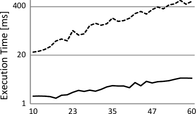
(a) Overall

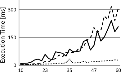
(b) Pipeline Stages

Figure 6: Execution time plotted against the number of nodes $n$. For each $n$ 10 graphs were generated randomly with an average of $1.5$ outgoing edges per node. (a) Overall execution time of KLay Layered (solid line) and CoDaFlow (dashed line). (b) Execution time of the pipeline steps: Untangling (solid line), Alignment (dashed line), and Edge Routing (dotted line). Timings were conducted on an Intel i7 2.0 GHz with 8 GB RAM.

Sect. 5 Conclusions

We present a novel approach to layout of data flow diagrams based on stress-minimization. We show that it is superior to previous approaches with respect to several diagram aesthetics. Also, it is more flexible and easier to implement.

The approach can easily be extended to further diagram types with similar drawing requirements, such as the Systems Biology Graphical Notation (SBGN). To allow interactive browsing of larger diagram instances, however, execution time has to be reduced, e. g., by removing overhead from both the implementation and the pipeline steps. Avoiding the crossing in Fig. 3 is currently not guaranteed. We plan to detect such obvious cases via ordering constraints. In addition to ACA, the use of topological improvement strategies [7] could help to reduce the number of edge bends further where edges are almost straight.

Acknowledgements.

Ulf Rüegg was funded by a doctoral scholarship (FIT-weltweit) of the German Academic Exchange Service. Michael Wybrow was supported by the Australian Research Council (ARC) Discovery Project grant DP110101390.

Appendix 0.A Appendix

0.A.1 Flat Graphs

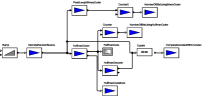
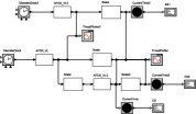
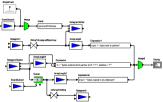
(a) CoDaFlow

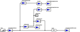
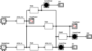
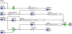
(b) KLay Layered

Figure 7: Comparison of the generated layouts of CoDaFlow and KLay Layered for flat graphs. Diagrams are taken from the Ptolemy example library: Huffman, AFDX, and Datagram (from top to bottom).

0.A.2 Compound Graphs

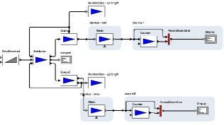
(a) CoDaFlow

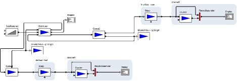
(b) KLay Layered

Figure 8: Comparison of the generated layouts for the Router diagram with 19 nodes, 24 edges, and 4 compound nodes.

(a) CoDaFlow

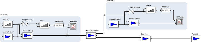
(b) KLay Layered

Figure 9: Comparison of the generated layouts for the dropqueuetest diagram with 16 nodes, 21 edges, and 2 compound nodes.

Appendix 0.B Computing ideal edge length to minimize $P$-stress

Let a graph $G=(V,E)$ be given, along with some linear ordering on $V$. We assume a layout of $G$ is already given, and regard its $P$-stress $P_{G}$ as a function of $\ell$:

$$P_{G}(\ell)=\sum_{u<v\in V}w_{uv}\left(\left(\ell p_{uv}-b(u,v)\right)^{+}\right)^{2}+\sum_{(u,v)\in E}\ell^{-2}\left(\left(b(u,v)-\ell\right)^{+}\right)^{2}$$

where $b(u,v)$ is the Euclidean distance between the boundaries of nodes $u$ and $v$ along the straight line connecting their centres, $p_{uv}$ the number of edges on the shortest path between nodes $u$ and $v$, $w_{uv}=(\ell p_{uv})^{-2}$, and $(z)^{+}=\max(z,0)$. We wish to compute the value of $\ell$ that minimises $P_{G}$.

We begin by rewriting the $P$-stress as:

$$P_{G}(\ell)=\sum_{(u,v)\in D}w_{uv}\left(\left(\ell p_{uv}-b(u,v)\right)^{+}\right)^{2}+\sum_{(u,v)\in E}\ell^{-2}\left(\ell-b(u,v)\right)^{2},$$

where $D=\{(u,v):u<v\wedge(u,v)\not\in E\wedge(v,u)\not\in E\}$. In other words, $D$ is simply the set of all ordered pairs written in ascending order, in which the nodes are not connected by an edge.

For each $(u,v)\in D$, define $\ell_{uv}=b(u,v)/p_{uv}$, and

$$h_{uv}(\ell)=\left\{\begin{array}[]{cl}\left(1-\frac{\ell_{uv}}{\ell}\right)^{2}&\ell\in[\ell_{uv},+\infty)\\ 0&\ell\in(0,\ell_{uv}].\end{array}\right.$$

Then $h_{uv}$ is in fact differentiable over $(0,+\infty)$, with

$$h_{uv}^{\prime}(\ell)=\left\{\begin{array}[]{cl}\frac{2\ell_{uv}}{\ell^{2}}\left(1-\frac{\ell_{uv}}{\ell}\right)&\ell\in[\ell_{uv},+\infty)\\ 0&\ell\in(0,\ell_{uv}],\end{array}\right.$$

and we have

$$P_{G}(\ell)=\sum_{(u,v)\in D}h_{uv}(\ell)+\sum_{(u,v)\in E}\left(1-\frac{b(u,v)}{\ell}\right)^{2}$$

and

$$P_{G}^{\prime}(\ell)=\sum_{(u,v)\in D}h_{uv}^{\prime}(\ell)+\sum_{(u,v)\in E}\frac{2b(u,v)}{\ell^{2}}\left(1-\frac{b(u,v)}{\ell}\right).$$

Now let $\langle\ell_{1},\ell_{2},\ldots,\ell_{\nu}\rangle$ be the list of all $\ell_{uv}$ for $(u,v)\in D$, written in non-decreasing order (some values may appear more than once). Since there may be repeated values among the $\ell_{i}$, let $\langle m_{1},m_{2},\ldots,m_{\mu}\rangle$ be the list of all distinct values of the $\ell_{i}$, written in strictly ascending order. For each $1\leq j\leq\mu$, let $A_{j}=\{i:\ell_{i}<=m_{j}\}$, and let $I_{j}=[m_{j},m_{j+1}]$. Restricting to the interval $I_{j}$ and substituting a new variable $\lambda_{j}$, we have

$$\left.P_{G}^{\prime}(\lambda_{j})\right|_{I_{j}}=\sum_{i\in A_{j}}\frac{2\ell_{i}}{\lambda_{j}^{2}}\left(1-\frac{\ell_{i}}{\lambda_{j}}\right)+\sum_{(u,v)\in E}\frac{2b(u,v)}{\lambda_{j}^{2}}\left(1-\frac{b(u,v)}{\lambda_{j}}\right),$$

and setting this derivative equal to zero and solving for $\lambda_{j}$, we find

$$\lambda_{j}=\frac{\sum_{(u,v)\in E}b(u,v)^{2}+\sum_{i\in A_{j}}\ell_{i}^{2}}{\sum_{(u,v)\in E}b(u,v)+\sum_{i\in A_{j}}\ell_{i}}.$$

This is simply the contraharmonic mean over $B\cup A_{j}$, where $B=\langle b(u,v):(u,v)\in E\rangle$; that is, the weighted mean in which the weights equal the values. For $\lambda_{j}$ to be an actual critical point of the function $P_{G}$ however, it must satisfy the assumption that it lies in the restricted interval $I_{j}$. Thus the ideal edge length $\bar{\ell}$ is found to be

$$\bar{\ell}=\operatorname*{arg\,min}_{\{\lambda_{j}:\lambda_{j}\in I_{j}\}}P_{G}(\lambda_{j}).$$

References

- [1] Brandes, U., Eiglsperger, M., Kaufmann, M., Wagner, D.: Sketch-driven orthogonal graph drawing. In: Proceedings of the 10th International Symposium on Graph Drawing (GD’02). LNCS, vol. 2528, pp. 1–11. Springer (2002)
- [2] Chimani, M., Gutwenger, C., Mutzel, P., Spönemann, M., Wong, H.M.: Crossing minimization and layouts of directed hypergraphs with port constraints. In: Proceedings of the 18th International Symposium on Graph Drawing (GD’10). LNCS, vol. 6502, pp. 141–152. Springer (2011)
- [3] Dwyer, T., Koren, Y., Marriott, K.: IPSep-CoLa: An incremental procedure for separation constraint layout of graphs. IEEE Transactions on Visualization and Computer Graphics 12(5), 821–828 (Sept 2006)
- [4] Dwyer, T., Lee, B., Fisher, D., Quinn, K.I., Isenberg, P., Robertson, G., North, C.: A comparison of user-generated and automatic graph layouts. IEEE transactions on visualization and computer graphics 15(6), 961–8 (2009)
- [5] Dwyer, T., Marriott, K., Stuckey, P.J.: Fast node overlap removal. In: Healy, P., Nikolov, N.S. (eds.) Proceedings of the 13th International Symposium on Graph Drawing (GD’05). LNCS, vol. 3843, pp. 153–164. Springer (2006)
- [6] Dwyer, T., Marriott, K., Wybrow, M.: Dunnart: A constraint-based network diagram authoring tool. In: Revised Papers of the 16th International Symposium on Graph Drawing (GD’08). LNCS, vol. 5417, pp. 420–431. Springer (2009)
- [7] Dwyer, T., Marriott, K., Wybrow, M.: Topology preserving constrained graph layout. In: Revised Papers of the 16th International Symposium on Graph Drawing (GD’08). LNCS, vol. 5417, pp. 230–241. Springer (2009)
- [8] Eades, P., Lin, X., Smyth, W.F.: A fast and effective heuristic for the feedback arc set problem. Information Processing Letters 47(6), 319–323 (1993)
- [9] Gansner, E.R., Koren, Y., North, S.C.: Graph drawing by stress majorization. In: Pach, J. (ed.) Graph Drawing. Lecture Notes in Computer Science, vol. 3383. Springer Berlin Heidelberg (2005)
- [10] Kieffer, S., Dwyer, T., Marriott, K., Wybrow, M.: Incremental grid-like layout using soft and hard constraints. In: Wismath, S., Wolff, A. (eds.) Graph Drawing. Lecture Notes in Computer Science, vol. 8242, pp. 448–459. Springer (2013)
- [11] Klauske, L.K.: Effizientes Bearbeiten von Simulink Modellen mit Hilfe eines spezifisch angepassten Layoutalgorithmus. Ph.D. thesis, Technische Universität Berlin (2012)
- [12] Klauske, L.K., Dziobek, C.: Improving modeling usability: Automated layout generation for Simulink. In: Proceedings of the MathWorks Automotive Conference (MAC’10) (2010)
- [13] Lee, E.A., Neuendorffer, S., Wirthlin, M.J.: Actor-oriented design of embedded hardware and software systems. Journal of Circuits, Systems, and Computers (JCSC) 12(3), 231–260 (2003)
- [14] Purchase, H.C.: Which aesthetic has the greatest effect on human understanding? In: Proceedings of the 5th International Symposium on Graph Drawing (GD’97). LNCS, vol. 1353, pp. 248–261. Springer (1997)
- [15] Schulze, C.D., Spönemann, M., von Hanxleden, R.: Drawing layered graphs with port constraints. Journal of Visual Languages and Computing, Special Issue on Diagram Aesthetics and Layout 25(2), 89–106 (2014)
- [16] Spönemann, M., Fuhrmann, H., von Hanxleden, R., Mutzel, P.: Port constraints in hierarchical layout of data flow diagrams. In: Proceedings of the 17th International Symposium on Graph Drawing (GD’09). LNCS, vol. 5849, pp. 135–146. Springer (2010)
- [17] Sugiyama, K., Tagawa, S., Toda, M.: Methods for visual understanding of hierarchical system structures. IEEE Transactions on Systems, Man and Cybernetics 11(2), 109–125 (Feb 1981)
- [18] Wybrow, M., Marriott, K., Stuckey, P.J.: Orthogonal connector routing. In: Proceedings of the 17th International Symposium on Graph Drawing (GD’09). LNCS, vol. 5849, pp. 219–231. Springer (2010)