A critical analysis of shock models for chondrule formation

Abstract

In recent years many models of chondrule formation have been proposed. One of those models is the processing of dust in shock waves in protoplanetary disks. In this model, the dust and the chondrule precursors are overrun by shock waves, which heat them up by frictional heating and thermal exchange with the gas.

In this paper we reanalyze the nebular shock model of chondrule formation and focus on the downstream boundary condition. We show that for large-scale plane-parallel chondrule-melting shocks the postshock equilibrium temperature is too high to avoid volatile loss. Even if we include radiative cooling in lateral directions out of the disk plane into our model (thereby breaking strict plane-parallel geometry) we find that for a realistic vertical extent of the solar nebula disk the temperature decline is not fast enough. On the other hand, if we assume that the shock is entirely optically thin so that particles can radiate freely, the cooling rates are too high to produce the observed chondrules textures. Global nebular shocks are therefore problematic as the primary sources of chondrules.

1 Introduction

The origin of chondrules is one of the biggest mysteries in meteoritics. These 0.1$\cdots$1 mm sized silicate once molten droplets, abundantly found in chondritic meteorites, must have cooled and solidified within a matter hours (e.g. Hewins et al., 2005). From short-lived radionuclide chronology data (e.g. Villeneuve et al., 2009) it is known that this must have taken place during the first few million years after the start of the solar system, during the phase when the sun was still likely surrounded by a gaseous disk (the “solar nebula”). What makes chondrule formation mysterious is that this few-hour cooling time is orders of magnitude shorter than the typical few-million-year time scale of evolution of the solar nebula. Chondrules can thus not be a natural product of the gradual cooling-down of the nebula. Instead, chondrules must have formed during “flash heating events” of some kind – but which kind is not yet known. There exists a multitude of theories as to what these flash heating events could have been. Boss (1996) and Ciesla (2005) give nice overviews of these theories and their pros and cons. So far none of these theories has been universally accepted.

One of the most popular theories is that nebular shock waves can melt small dust aggregates in the nebula, causing them to become melt droplets and allowing them to cool again and solidify (Hood and Horanyi, 1991). The origin of such shocks could, for instance, be gravitational instabilities in the disk (e.g. Boley and Durisen, 2008) or the effect of a gas giant planet (e.g. Kley and Nelson, 2012). Detailed 1-D models of the structure of such radiative shocks, and the formation of chondrules in them, were presented by Iida et al. (2001), Desch and Connolly (2002), Ciesla and Hood (2002) or Morris and Desch (2010). These models show that such a shock, in an optically thick solar nebula, would lead to a temperature spike in the gas and the dust that lasts for only a few seconds to minutes with cooling rates of up to $10^{3}$ K/hour, followed by a more gradual cooling lasting several hours, with cooling rates of the order of $50$ K/hour. These appear to be the right conditions for chondrule formation, which is one of the reasons why this model is one of the favored models of chondrule formation nowadays.

In this paper we revisit this shock-induced chondrule formation model. Our aim is to investigate the role of the downstream boundary condition and the role of sideways radiative cooling.

If the shock is a large scale shock, e.g. due to a global gravitational instability, then on a small scale (the scale of several radiative mean free paths $\lambda_{\mathrm{free}}$) the shock can be modeled as a infinite 1-D radiation hydrodynamic flow problem. The “infinite 1-D” in this context means that the 3-D geometry of the problem only becomes important on scales $\gg\lambda_{\mathrm{free}}$, so that on scales $\sim\lambda_{\mathrm{free}}$ a 1-D geometry can be safely assumed where the pre-shock boundary is set at $x=-\infty$ and the post-shock boundary is set at $x=+\infty$. With $\lambda_{\mathrm{free}}=\left(\kappa\rho\right)^{-1}$ the pressure scale height of a typical minimum mass solar nebula is several hundred times larger than the optical mean free path. The shock is assumed to be stationary in the $x$-coordinate system, i.e. the coordinates move along with the shock and the shock is always at $x=0$. In such an infinite 1-D system the full shock structure can be reconstructed when the physical variables at the upsteam boundary $x=-\infty$ are all given. No downsteam boundaries at $x=+\infty$ need to be given. In fact, the physical variables at $x=+\infty$ follow uniquely by demanding that the mass-, momentum- and energy-flux at $x=+\infty$ equals those of $x=-\infty$, but with subsonic gas velocity at $x=+\infty$. This gives a global Rankine-Hugoniot condition including all the radiative and dust physics. Note that right at the shock at $x=0$ the jump in the gas variables is given by a local Rankine-Hugoniot condition in which only the gas fluxes on both sides are set equal. We will work out these shock models in section 2 and show that after the temperature spike they lack a slower few-hour cooling phase. Instead, they stay at a constant temperature, i.e. the temperature in accordance with the global Rankine-Hugoniot condition. We will investigate in section 3.1 whether the chondrule peak temperature can be made high enough for melting while keeping the post-spike temperature low enough to retain volatile elements. According to Fedkin et al. (2012) and Yu et al. (1996) the high-temperature phase should be of the order tens of minutes rather than of hours. From textural constraints, Hewins et al. (2005) and Desch et al. (2012) conclude that the cooling rates have to be of the order of 10¹ – 10³ K/hour.

Since the infinite 1-D shock solution is a geometric approximation we will implement effects of sideways cooling (i.e., from top and bottom of the disk) in section 3.2 to improve the realism of the model. This will re-introduce the slow cooling phase after the temperature spike, but we find that this slow cooling phase is of the order of weeks/months/years rather than hours, because 2-D/3-D radiative diffusion will take place on $x$-scales of the same order as the vertical scale height of the disk.

Finally we discuss in section 3.3 two versions of the shock-induced chondrule formation where the cooling time can be rapid. One is a locally induced one, for instance due to a supersonic planetesimal bow shock (Hood, 1998; Morris et al., 2012). The other is if the disk is fully optically thin, allowing the post-shock material to cool straight to infinity.

2 The Model

Our one-dimensional shock model is built on the work by Desch and Connolly (2002). We used their approach, generalized it to arbitrarely many gas species, particle populations and chemical reactions and modified it where we think modifications or corrections are needed.

In this model we assume that all the parameters (densities, temperatures, velocities, etc.) only change along one direction, the $x$-direction. Therefore, the model consists of infinitely extended, plane-parallel layers of constant temperatures, velocities and densities.

2.1 Radiative Transfer

Even though the model is one-dimensional, we must allow the photons to move into all three directions. But fortunately, because of the plane-parallel assumption the radiative transfer equations here can be vastly simplified.

In this case the optical depth $\tau$ is a monotonic increasing function of the distance from the post-shock boundary and therefore a meassure of the position $x$ inside the computational domain:

$$\tau\left(x\right)=\int\limits_{x}^{x_{\mathrm{post}}}\alpha\mathrm{d}x,$$ (1)

where $x_{\mathrm{post}}$ is the location of the post-shock boundary. This means the optical depth increases from $\tau\left(x_{\mathrm{post}}\right)=0$ at the post-shock boundary to a maximum value of $\tau\left(x_{\mathrm{pre}}\right)=\int\limits_{x_{\mathrm{pre}}}^{x_{\mathrm{post}}}\alpha\mathrm{d}x\equiv\tau_{\mathrm{max}}$ at the pre-shock boundary. $\alpha$ is the absorption coefficient, which is the sum of the contribution of the gas and the particles:

$$\begin{split}\alpha&=\alpha_{\mathrm{g}}+\alpha_{\mathrm{p}}\\ &=\rho_{\mathrm{g}}\kappa_{\mathrm{P}}+n\pi a^{2}\varepsilon.\end{split}$$ (2)

The absoption coefficient of the gas is the product of the gas mass density $\rho_{\mathrm{g}}$ and the temperature-dependent Planck-mean opacity $\kappa_{\mathrm{P}}$, which we took from Semenov et al. (2003) (see figure 1). The absorption coefficient of the particles is the product of their number densities $n$, their geometrical cross-section and their absoprtion efficiency $\varepsilon$, which we adopted from Desch and Connolly (2002) as

$$\varepsilon=0.8\times\mathrm{min}\left[1,\ \left(\frac{a}{2\ \mu\mathrm{m}}\right)\right],$$ (3)

where $a$ is the particle radius.

Figure 1: Planck-mean opacity from Semenov et al. (2003). At $\sim 1350$ K (vertical line) the fine-grained dust associated with the gas gets evaporated. Therefore, the opacity drops by one order of magnitude at this temperature. This is responsible for the “opacity knee” in the pre-heating phase, where the gas becomes optically thin.

To calculate the thermal histories of the particles one has to calculate the mean intensity $J_{\mathrm{rad}}\left(\tau\right)$ at every position $\tau$ Our radiative transfer is grey, i.e. wavelength independent. The mean intensity is defined as the average intensity $I$ per solid angle coming from all directions

$$J_{\mathrm{rad}}\left(\tau\right)=\frac{1}{4\pi}\int\limits_{\Omega}I\left(\tau,\mu\right)\mathrm{d}\Omega.$$ (4)

In the plane-parallel assumption the intensity depends only on the position $\tau$ and the angle $\theta$ between the incoming ray and the $x$-axis. $\mu$ is defined as $\mu=\cos\theta$. Therefore, the mean intensity can be simplified to

$$\begin{split}J_{\mathrm{rad}}\left(\tau\right)=&\frac{I_{\mathrm{pre}}}{2}E_{2}\left(\tau_{\mathrm{max}}-\tau\right)+\frac{I_{\mathrm{post}}}{2}E_{2}\left(\tau\right)\\ &+\frac{1}{2}\int\limits_{0}^{\tau_{\mathrm{max}}}S\left(\tau^{\prime}\right)E_{1}\left(\left|\tau^{\prime}-\tau\right|\right)\mathrm{d}\tau^{\prime},\end{split}$$ (5)

by using the exponential integrals

$$E_{n}\left(x\right)=\int\limits_{1}^{\infty}\frac{e^{-xt}}{t^{n}}\mathrm{d}t,$$ (6)

(see Mihalas and Weibel-Mihalas, 1999). $I_{\mathrm{pre}}=\frac{\sigma}{\pi}T_{\mathrm{pre}}^{4}$ and $I_{\mathrm{post}}=\frac{\sigma}{\pi}T_{\mathrm{post}}^{4}$ are the incoming radiations from both boundaries. The source function $S\left(\tau\right)$ is defined as

$$S=\frac{\rho_{\mathrm{g}}\kappa_{\mathrm{P}}B\left(T_{\mathrm{g}}\right)+n\pi a^{2}\varepsilon B\left(T\right)}{\rho_{\mathrm{g}}\kappa_{\mathrm{P}}+n\pi a^{2}\varepsilon},$$ (7)

which are the wave-length integrated Plank functions $B\left(T\right)=\left(\sigma/\pi\right)T^{4}$ of the gas and the particles at their given temperatures weighted by their respective emission efficiencies, which are the same as their absoprtion efficiencies according Kirchoff’s law. $\sigma$ is the Stefan-Boltzmann constant.

The radiative flux $F_{\mathrm{rad}}$ is defined as the net flux of radiative energy in $x$-direction

$$\begin{split}F_{\mathrm{rad}}&=-\int\limits_{\Omega}I\left(\tau,\mu\right)\cos\theta\mathrm{d}\Omega\\ &=-2\pi\int\limits_{-1}^{1}I\left(\tau,\mu\right)\mu\mathrm{d}\mu.\end{split}$$ (8)

Later, we need the derivative of the radiative flux with respect to the $x$-direction. In the plane-parallel assumption this is simply

$$\begin{split}\frac{\partial F_{\mathrm{rad}}}{\partial x}=&-4\pi\alpha\left(J_{\mathrm{rad}}-S\right)\\ =&-4\pi\rho_{\mathrm{g}}\kappa_{\mathrm{P}}\left(J_{\mathrm{rad}}-\frac{\sigma T_{\mathrm{g}}^{4}}{\pi}\right)\\ &-4\pi\sum\limits_{j=1}^{N_{J}}n_{j}\pi a_{j}^{2}\varepsilon_{j}\left(J_{\mathrm{rad}}-\frac{\sigma T_{\mathrm{j}}^{4}}{\pi}\right),\end{split}$$ (9)

where we now included $N_{J}$ different particle populations. Therefore, we have to take the sum over all populations.

2.2 Hydrodynamics

To calculate the evolution of the gas and particle parameters we used the one-dimensional stationary Euler equations, which are

$$\partial_{x}\left[\rho V\right] =S_{\rho}$$ (10)

$$\partial_{x}\left[\rho V^{2}+P\right] =S_{p}$$ (11)

$$\partial_{x}\left[\left(\rho e_{\mathrm{tot}}+P\right)V\right] =S_{e},$$ (12)

with the total mass density $\rho$, the velocity $V$, the pressure $P$ and kinetic and thermal energy density $e_{\mathrm{tot}}$. These equations are simply conservation laws of mass, momentum and energy respectively. S_ρ, S_p and S_e are the source terms of the designated quantities.

2.2.1 Particle dynamics

In this model we have $N_{J}$ different particle populations with radius $a_{j}$, temperature $T_{j}$, velocity $V_{j}$ and number density $n_{j}$. The particles are not allowed to evaporate completely. This means the continuity equation (10) states

$$\partial_{x}\left[n_{j}V_{j}\right]=0.$$ (13)

The particles are accelerated or decelerated by the drag force $F_{\mathrm{drag},j}$ acting on population $j$. The drag force is given by

$$F_{\textrm{drag},j}=-\pi a_{j}^{2}\rho_{\mathrm{g}}\frac{C_{\mathrm{D},j}}{2}\left|V_{j}-V_{\mathrm{g}}\right|\left(V_{j}-V_{\mathrm{g}}\right)$$ (14)

(Gombosi et al., 1986), with the gas’ mass density $\rho_{\mathrm{g}}$ and the drag coefficient $C_{\mathrm{D},j}$ of population $j$ (see A for futher details). If the gas velocity is higher than the particle velocity, the particles get accelerated and vice versa. With that, the force equation of the particles is

$$m_{j}\frac{\mathrm{D}}{\mathrm{D}t}V_{j}=F_{\mathrm{drag},j},$$ (15)

with the particles’ mass $m_{j}$ and the comoving derivative $\mathrm{D}/\mathrm{D}t$, which is defined as

$$\frac{\mathrm{D}}{\mathrm{D}t}\equiv\frac{\partial}{\partial t}+\vec{V}_{j}\cdot\vec{\nabla}=V_{j}\frac{\partial}{\partial x}.$$ (16)

The last equality is for the one-dimensional, stationary case. Using this, the force equation (15) yields

$$m_{j}V_{j}\frac{\partial}{\partial x}V_{j}=F_{\mathrm{drag},j}.$$ (17)

The energy budget of the particles is given by the balance between frictional heating by the gas drag, thermal contact with the gas and radiative heating on one hand and radiative cooling on the other hand. The effects of frictional heating and thermal contact with the gas are combined into a single heating rate $q_{j}$ per unit surface area of the particle given by

$$q_{j}=\rho_{\mathrm{g}}C_{\mathrm{H},j}\left(T_{\mathrm{rec}}-T_{j}\right)\left|V_{\mathrm{g}}-V_{j}\right|$$ (18)

(Gombosi et al., 1986), with the heat transfer coefficient $C_{\mathrm{H},j}$ and the recovery temperature $T_{\mathrm{rec}}$. In the limit of $V_{\mathrm{g}}=V_{\mathrm{j}}$ there can be still heat exchange if $T\mathrm{g}\neq T\mathrm{j}$ (see A for further details). The radiative heating rate per unit surface area of the paticles is given by $\varepsilon_{j}\left(\pi J_{\mathrm{rad}}-\sigma T_{j}^{4}\right)$, which is the balance between radiation received by the mean intensity $J_{\mathrm{rad}}$ and the energy radiated away according the Stefan-Boltzmann law. Combining the effects of frictional and thermal heating and radiative heating the net heating rate per unit surface area is $q_{j}+\varepsilon_{j}\left(\pi J_{\mathrm{rad}}-\sigma T_{j}^{4}\right)$.

This net heating rate can raise the particles’ temperatures and/or evaporate them. We assume that the fraction of the net heating rate that goes into evaporation is $f_{\mathrm{evap},j}$, which is a function of the particle temperature. $f_{\mathrm{evap},j}$ increases monotonically from 0 to 1 within a temperature interval $\Delta T$ centered on the evaporation temperature of 2000 K used by Desch and Connolly (2002). We have arbitrarely chosen $\Delta T=100~{}\mathrm{K}$ (see figure 2). We had to do this because of numerical reasons (strong if-statements can make it impossible to estimate the Jacobian for the implicit integration scheme), but the positive side effect is that we can account now for the heterogeneity of the particle material with different evaporation temperatures.

Figure 2: The fraction of evaporation $f_{\mathrm{evap}}$ yields for a smearing of the evaporation temperature of 2000 K within our choice of the interval $\Delta T=100~{}\mathrm{K}$.

Therefore, the change in the particles’ temperature is given by

$$\begin{split}m_{j}C_{\mathrm{P},j}\frac{\mathrm{D}}{\mathrm{D}t}T_{j}=&\left(1-f_{\mathrm{evap},j}\right)\times\\ &\times 4\pi a_{j}^{2}\left[q_{j}+\varepsilon_{j}\left(\pi J_{\mathrm{rad}}-\sigma T_{j}^{4}\right)\right],\end{split}$$ (19)

with the specific heat capacity at constant pressure $C_{\mathrm{P},j}$ of the particle material. Using again the definition of the comoving derivative (16), the particles’ material mass density $\rho_{j}$ and using $m_{j}=4/3\pi\rho_{j}a_{j}^{2}$ the change in the particles’ temperature can be written as

$$\frac{\partial}{\partial x}T_{j}=\frac{3\left(1-f_{\mathrm{evap},j}\right)}{\rho_{j}a_{j}V_{j}C_{\mathrm{P},j}}\left[q_{j}+\varepsilon_{j}\left(\pi J_{\mathrm{rad}}-\sigma T_{j}^{4}\right)\right].$$ (20)

The other part of the net heating rate, that goes into evaporation, is given by

$$\begin{split}H_{\mathrm{evap},j}\frac{\mathrm{D}}{\mathrm{D}t}m_{j}=&-f_{\mathrm{evap},j}\times\\ &\times 4\pi a_{j}^{2}\left[q_{j}+\varepsilon_{j}\left(\pi J_{\mathrm{rad}}-\sigma T_{j}^{4}\right)\right],\end{split}$$ (21)

with the latent heat of evaporation $H_{\mathrm{evap},j}$ of the particle material. The negative sign is needed because the heat received here goes into shrinking the particles’ mass. This yields for the change in the particle radius

$$\frac{\partial}{\partial t}a_{j}=-\frac{f_{\mathrm{evap},j}}{\rho_{j}H_{\mathrm{evap},j}V_{j}}\left[q_{j}+\varepsilon_{j}\left(\pi J_{\mathrm{rad}}-\sigma T_{j}^{4}\right)\right].$$ (22)

If the net heating rate is negative then $f_{\mathrm{evap},j}$ is set to zero to avoid artificial condensation in equation (22). We neglect condensation and nucleation here because we assume it takes place on much longer timescales than considered here. We want to point out that this implementation of evaporation is not the correct physical treatment. To do it in an correct way one has to integrate the Hertz-Knudsen equation and possibly a nucleation model, which makes the whole system even more complex. We also want to point out that in our conclusive simulations, the particle temperature is always safely below the evaporation temperature.

With the continuity equation of the particles (13) and the change in the particle velocity (17), the change in the particles’ number densities can be calculated

$$\frac{\partial}{\partial x}n_{j}=-\frac{n_{j}}{V_{j}}\frac{\partial}{\partial x}V_{j}.$$ (23)

With equations (17), (20), (22) and (23) all the particle parameters can be calculated throughout the computational domain knowing the gas parameters.

2.2.2 Gas Dynamics

The gas consists of $N_{I}$ different gas species, which are assumed to be well-coupled and share the same temperature $T_{g}$ and velocity $V_{g}$. Each species $i$ has a number density $n_{i}$ (do not confuse this with $n_{j}$ of the particles) and a mean molecular weight $m_{i}$.

The model also includes $N_{K}$ different chemical reactions with their respective net reaction rates $R_{k}$ of reaction $k$, which are the number of reactions per unit time per unit volume. In chemical equilibrium the net reactions rates are equal to zero (which does not mean that no chemical reaction takes place).

Every reaction costs or sets free energy. The definition is such, that a positive reaction rate $R_{k}$ sets free the energy $e_{k}$. That means that the total energy per unit time and unit volume set free by reaction $k$ is $R_{k}e_{k}$. With chemistry the continuity equations of the different gas species are

$$\frac{\partial}{\partial x}\left(n_{i}V_{\mathrm{g}}\right)=\sum_{k=0}^{N_{K}}R_{i,k},$$ (24)

where $R_{i,k}$ is the creation rate of gas species $i$ due to reaction $k$ (i.e., the change in number density $n_{i}$ due to reaction k). The $k=0$ component of the creation rates $R_{i,0}$ accounts for changes due to non-chemical processes, e.g. evaporation since the mass of the evaporated material has to be added to the gas.

The total mass loss per unit time and unit volume of all particle populations is

$$\sum_{j=1}^{N_{J}}n_{j}\frac{\mathrm{D}}{\mathrm{D}t}m_{j}=\sum_{j=1}^{N_{J}}n_{j}V_{j}4\pi\rho_{j}a_{j}^{2}\frac{\partial}{\partial x}a_{j}.$$ (25)

This mass has to be added to the different gas species via the $k=0$ component of their creation rates

$$R_{i,0}=-\frac{\xi_{\mathrm{evap},i}}{m_{i}}\sum_{j=1}^{N_{J}}n_{j}V_{j}4\pi\rho_{j}a_{j}^{2}\frac{\partial}{\partial x}a_{j},$$ (26)

where $\xi_{\mathrm{evap},i}$ is the fraction of the evaporated mass added to gas species $i$. For mass conservation $\sum\limits_{i}\xi_{\mathrm{evap},i}=1$ has to hold.

To close the system of equations one has to solve for the gas temperature $T_{\mathrm{g}}$, the gas velocity $V_{\mathrm{g}}$ and the number densities $n_{i}$. To do so we use Euler’s momentum equation (11) and sum up the total momentum of the gas and the particles

$$\begin{split}\frac{\partial}{\partial x}\left[\sum_{i=1}^{N_{I}}\left(\rho_{i}V_{\mathrm{g}}^{2}+n_{i}k_{\mathrm{B}}T_{\mathrm{g}}\right)+\sum_{j=1}^{N_{J}}n_{j}m_{j}V_{j}^{2}\right]=0.\end{split}$$ (27)

The first term in the sum over $i$ is the momentum carried by the gas, the second term is the pressure according the ideal gas law. The sum over $j$ refers to the momentum carried by the particles. Since the particles are pressureless there is no pressure term. This formula can be manipulated to get to

$$\begin{split}&\left(\rho_{\mathrm{g}}V_{\mathrm{g}}-\frac{k_{\mathrm{B}}T_{\mathrm{g}}}{V_{\mathrm{g}}}\sum_{i=1}^{N_{I}}n_{i}\right)\frac{\partial}{\partial x}V_{\mathrm{g}}+\left(k_{\mathrm{B}}\sum_{i=1}^{N_{I}}n_{i}\right)\frac{\partial}{\partial x}T_{\mathrm{g}}\\ =&-\sum_{j=1}^{N_{J}}n_{j}\left(F_{\mathrm{drag},j}+4\pi a_{j}^{2}\rho_{j}V_{j}^{2}\frac{\partial}{\partial x}a_{j}\right)\\ &-\sum_{i=1}^{N_{I}}\sum_{k=0}^{N_{K}}R_{i,k}\left(V_{\mathrm{g}}m_{i}+\frac{k_{\mathrm{B}}T_{\mathrm{g}}}{V_{\mathrm{g}}}\right)\end{split}$$ (28)

(see B for detailed calculations).

The same kind of calculations can be done for Euler’s energy equation (12)

$$\begin{split}&\frac{\partial}{\partial x}\left[\sum_{i=1}^{N_{I}}n_{i}V_{\mathrm{g}}\left(\frac{m_{i}V_{\mathrm{g}}^{2}}{2}+\frac{f_{i}+2}{2}k_{\mathrm{B}}T_{\mathrm{g}}\right)\right.\\ &\left.+\sum_{j=1}^{N_{J}}n_{j}m_{j}V_{j}\left(\frac{V_{j}^{2}}{2}+C_{\mathrm{P},j}T_{j}\right)+F_{\mathrm{rad}}\right]\\ =&\sum_{k=0}^{N_{K}}R_{k}e_{k}.\end{split}$$ (29)

The first term in the sum over $i$ is the kinetic energy carried by the gas, whereas the second term is the sum of the internal energy of the gas and the pressure term according the ideal gas law. $f_{i}$ is the number of degrees of freedom of gas species $i$. The first term in the sum over $j$ is the kinetic energy carried by the particles, the second term is the thermal energy of the particles. In addition to that the radiative flux $F_{\mathrm{rad}}$ has to be included. The right hand side is not equal to zero, because energy can be created or consumed by chemical reactions. This equation can be further manipulated to

$$\begin{split}&V_{\mathrm{g}}^{2}\sum_{i=1}^{N_{I}}n_{i}m_{i}\frac{\partial}{\partial x}V_{\mathrm{g}}+k_{\mathrm{B}}V_{\mathrm{g}}\sum_{i=1}^{N_{I}}n_{i}\frac{f_{i}+2}{2}\frac{\partial}{\partial x}T_{\mathrm{g}}\\ =\quad&4\pi\rho_{\mathrm{g}}\kappa\left(J_{\mathrm{rad}}-\frac{\sigma T_{\mathrm{g}}^{4}}{\pi}\right)+4\pi\sum_{j=1}^{N_{J}}n_{j}\pi a_{j}^{2}\varepsilon_{j}\left(J_{\mathrm{rad}}-\frac{\sigma T_{j}^{4}}{\pi}\right)\\ &-\sum_{i=1}^{N_{I}}\sum_{k=0}^{N_{K}}R_{i,k}\left(\frac{m_{i}V_{\mathrm{g}}^{2}}{2}+k_{\mathrm{B}}T_{\mathrm{g}}\frac{f_{i}+2}{f_{i}}\right)\\ &-\sum_{j=1}^{N_{J}}n_{j}V_{j}\left(F_{\mathrm{drag},j}+2\pi V_{j}^{2}\rho_{j}a_{j}^{2}\frac{\partial}{\partial x}a_{j}\right)\\ &-\sum_{j=1}^{N_{J}}n_{j}V_{j}m_{j}C_{\mathrm{P},j}\frac{\partial}{\partial x}T_{j}\\ &-4\pi\sum_{j=1}^{N_{J}}n_{j}V_{j}C_{\mathrm{P},j}T_{j}a_{j}^{2}\rho_{j}\frac{\partial}{\partial x}a_{j}\\ &+\sum_{k=1}^{N_{K}}R_{k}e_{k}\end{split}$$ (30)

(see B for detailed calculations).

Equations (28) and (30) are a set of two coupled differential equations, which can be solved for $\frac{\partial}{\partial x}V_{\mathrm{g}}$ and $\frac{\partial}{\partial x}T_{\mathrm{g}}$. Together with the continuity equation (24) of the gas and the particle differential equations (17), (20), (22) and (23) this closes the system of equations.

Setting $N_{I}=4$ and using the gas species $\mathrm{H}$, $\mathrm{H_{2}}$, $\mathrm{He}$ $\mathrm{and}$ $\mathrm{SiO}$ this reduces in principle to the model of Desch and Connolly (2002), but correcting for some sign errors and implementing the smooth transition of the evaporation temperature.

2.3 Numerical Method

The system of equations (17), (20), (22), (23), (24), (28) and (30) is extremely stiff. Therefore it would require a very small step size and a very large number of grid points to numerically integrate it with an explicit integration scheme. We used here the implicit integrator DVODE (Brown et al., 1989) to integrate the equations simultaneously through the computational domain.

We performed our calculations in the comoving frame of the shock front, which is set to be at $x=0$. At the shock front the gas parameters are changed according the Rankine-Hugoniot jump conditions, while the particle parameters remain unchanged.

After every complete integration the radiative transfer calculations have to be done again with the new particle and gas parameters. Then the integration is repeated with these new radiative parameters. This is repeatedly done until convergence is reached.

Another crucial point is the calculation of the post-shock boundary temperature $T_{\mathrm{post}}$, which is needed for the radiative transfer calculation. Desch and Connolly (2002) calculated $T_{\mathrm{post}}$ by using incorrect jump conditions adopted from Hood and Horanyi (1991). This was corrected by Morris and Desch (2010) by calculating their own jump conditions. They found post-shock temperatures on the order of $>1300~{}\mathrm{K}$ and concluded that chondrule formation is not possible in strictly one-dimensional models. Since disks are not one-dimensional objects they will eventually cool by radiation. Therefore Morris and Desch (2010) loosened the one-dimensional assumption by setting the post-shock temperature to the pre-shock temperature $T_{\mathrm{post}}=T_{\mathrm{pre}}$. This approach raises a problem, however, since it forces the gas and dust to radiatively cool through the downstream boundary. Since this downstream boundary is not a physical boundary, but just a computational boundary, this does not appear to be justified. The cooling is then dependent on the distance between shock front and post-shock boundary.

In our model we do not set the post-shock temperature a-priori since in a one-dimensional stationary model all downstream parameters are completely set by the upstream conditions. Therefore we perform right before the first iteration an additional integration without radiation. The temperature reached there at the post-shock boundary is then used as a first approximation of the post-shock temperature. After every further iteration, we check the radiative flux through the post-shock boundary. If the flux is positive i.e., the final temperature is higher than the post-shock temperature, we increase $T_{\mathrm{post}}$ slightly and vice versa. If convergence is reached then the radiative flux at the post-shock boundary is equal to zero. We want to point out that $F_{\mathrm{rad}}=0$ is only true at the boundaries, which have to be at large enough $|x|$.

The post-shock temperatures we found by this approach are even higher than those calculated by Morris and Desch (2010). We think this is due to some approximations performed in deriving their jump conditions. Later in section 3 we introduce a method to perform simulations with a vertical energy loss.

3 Results

For reasons of comparison we used the same input parameters as Desch and Connolly (2002), which we want to repeat here.

We have one particle population with initial radius of 300 $\mu$m and an material mass density of 3.3 g/cm³. Their initial number density can then be calculated by assuming a gas density of $10^{-9}$ g/cm³, a dust-to-gas ratio of 0.005 and assuming that 75 % of the dust mass are in the chondrule precursors. The particles have a heat capacity of $C_{\mathrm{P}}=10^{7}$ erg/g/K. Between 1400 K and 1820 K melting takes place. This results in an effective heat capacity of $C_{\mathrm{P}}=2.19\cdot 10^{7}$ erg/g/K within this temperature interval (see Desch and Connolly, 2002, and references therein for detailed descriptions). The latent heat of evaporations is $H_{\mathrm{evap}}=1.1\cdot 10^{11}$ erg/g.

The intial temperature of both gas and dust is 300 K. The gas consists of four species: atomic hydrogen, molecular hydrogen, helium and silicon monoxide (SiO). The only chemical reaction we consider is hydrogen dissociation and recombination, which consumes 4.48 eV for every H₂ molecule that breaks apart. We used the reaction rates given in Desch and Connolly (2002) adopted from Cherchneff et al. (1992). The reaction can also go in reverse direction; then setting free energy. If the gas exceeds 1350 K, then the dust associated with it evaporates. The mass of the evaporated dust gets added to the silicon monoxide.

3.1 The standard shock

Figure 3: Left: Particle temperature in a shock with shock speed $V_{\mathrm{shock}}=6.5$ km/s. Right: Same as left but with gas temperature. See text for further description.

A standard shock with a shock speed of $V_{\mathrm{shock}}=6.5$ km/s is shown in figure 3. Most of the time the gas and the particles are well-coupled and share the same temperature. Already 3-4 hours before the shock front, the particles receive radiation from the hot gas and particles behind the shock. The temperature increases rapidly until roughly 1350 K. From that point on the temperature only slightly increases towards the shock front. This change in slope is related to the opacity (see figure 1). As the gas reaches temperatures of $\sim$ 1350 K the fine grained dust associated with the gas gets evaporated and the opacity drops by one order of magnitude. From that point on the opacity is purely caused by molecular lines. Therefore the pre-heating region can be sub-divided into an optically thick and an optically thin region. It is important that the opacity is not set to zero because then the gas could not actively cool anymore. The only chance to lose energy would then be thermal contact with the particles. This would artificially slow down the cooling process.

At the position of the shock front the parameters of the gas only are changed (i.e., without radiation or dust) according the Rankine-Hugoniot jump conditions wheareas the particle parameters remain unchanged. Therefore, the gas reaches temperatures as high as 2700 K. The particles suddenly find themselves surrounded by gas that is much hotter than before the shock and that has velocities much smaller than those of the particles. The particles are now heated up by thermal contact with the hot gas and by frictional heating. But since the radiative cooling into the pre-shock region is relatively effective, both the gas and the particles quickly reach an equilibrium post-shock temperature before the particles are able to adapt to the high gas temperatures. In that way the maximum temperature the particles reach is $\sim 1000$ K smaller than the maximal gas temperature.

The constant post-shock equilibrium temperature is a consequence of the one-dimensionality of the model. As soon as the gas and the particles are a few optical depths behind the shock front there is no way for them to lose energy into the pre-shock region by radiation. Since the model consists of infinitely extended plane-parallel layers, they can not cool in lateral directions.

Therefore our model has in principle two different jump conditions: one is local at the position of the shock front, where only the gas parameters are changed according the Rankine-Hugoniot jump conditions. The other global jump condition forces the gas and particles to be at rather high post-shock temperatures after the relaxation of the temperature spike at the shock front.

From now on the maximum temperature the particles experience in the spike is referred to as peak temperature $T_{\mathrm{peak}}$, whereas the equilibrium post-shock temperature is $T_{\mathrm{post}}$.

The results for different shock speeds look similar. The lower the shock speed, the lower $T_{\mathrm{peak}}$ and $T_{\mathrm{post}}$ and the smaller the pre-heating region. Only if the shock speed is too low for the gas to reach 1350 K, then there’s also a lack of the “opacity knee” noticable.

The chemical reaction of hydrogen dissociation works as energy sink in this case. Instead of raising the temperature, energy is consumed in breaking molecular bonds. Simulations without chemical reactions show an overall increase in temperature downstream by $\sim 100$ K. We want to point out that only a small fraction of the H₂ is dissociated. This demonstrates that it is very important to include chemistry in such simulations: the temperature deviation can make the difference between losing particles via evaporation or not. Whether or not other chemical reactions are equaly important has to be investigated.

Figure 4: Cooling rates of the particles at particle temperatures T $>1500$ K in the standard shock

Figure 4 shows the cooling rates of the particles in the standard shock at temperatures T $>1500$ K which is the important temperature regime for crystallization. As seen here the peak of the cooling rates is at the upper limit of what is allowed by experimental constraints. The standard shock itself is too weak to completely melt the particles. In addition to that the cooling rates drop to zero at already  1600 K. This is discussed later in this section.

Figure 5: Velocity of the particles.

Another interesting feature is shown in figure 5: the velocity of the particles in the simulation. As soon as the pre-heating sets in the particles’ velocity decreases because the gas velocity decreases. From initially $6.5$ km/s to roughly $5.5$ km/s shortly before the shock front. After the gas velocity is changed according the Rankine-Hugoniot conditions at the shock front the particles are rapidly decellerated by the drag force within minutes to $\sim 1.0$ km/s.

The Mach number of the gas is initially of the order of 5. But due to the increase in temperature and decrease in velocity it is only roughly 2 at the position of the shock, where the Mach number is applied in the Rankine-Hugoniot conditions.

Figure 6: The peak and post-shock temperatures of the standard shock for different shock speeds. The upper solid line denotes a temperature of 1820 K, which we assume the particles have to reach to be completely molten. The lower solid line is at 1400 K. This is the temperature the particles have to reach at least after the shock to retain their volatiles. This is not possible in the standard case.

Figure 7: Same as figure 6 but with higher gas mass densities of 10^-8 g/cm³ (left) and 10^-7 g/cm³ (right).

The problem of chondrule formation within this scenario is summarized in figure 6. If we assume that the particles have to reach a temperature of at least 1820 K to be completely molten and at the same time to cool rapidly back down below at least 1400 K to retain volatile materials which are observed in them, this is not possible in a one-dimensional model of an optically thick disk.

If we increase the gas mass density (see figure 7) the problem improves slightly and the two lines of peak and post-shock temperature are further apart. But only at unrealistic densities of $\gtrsim 10^{-6}$ g/cm³ we could have both requirements fulfilled at the same time. According the disk model by Bell et al. (1997) these high midplane densities can only be found at radii of $\sim 0.001$ AU or closer to the sun, where the temperatures are already on the order of 10³ K to 10⁴ K depending on the accretion rate.

But we want to point out that post-shock temperatures of 1400 K might already be too high to retain the volatiles. In addition to that the particles are already at high temperatures in the pre-heating phase for a prolonged time ($\sim$ 3 h for the standard shock, cf. figure 3), which is already too long to be consistent with chondrule formation (Fedkin et al., 2012).

3.2 Vertical energy loss

It is clear that a one-dimensional, plane-parallel model does not match the situation in actual protoplanetary disks, since such disks are not one-dimensional objects. They have a vertical extent with decreasing densities at higher altitudes above the midplane. At $R=3$ AU (the region of the asteroid belt where most of the chondrules can be found today) the pressure scale height of a disk around a solar mass star with a midplane temperature of $T=300$ K is $H_{\mathrm{P}}=\frac{k_{\mathrm{B}}TR^{3}}{\mu m_{\mathrm{p}}GM_{\odot}}\simeq 0.1$ AU, with the mean molecular weight of the gas $\mu\simeq 2.2$ amu and the proton mass $m_{\mathrm{p}}$.

If the disk is heated up by a shock whose propagation direction lies in the plane of the disk it can cool in vertical direction by radiative diffusion. But to cool down to the pre-shock temperature the gas and particles have to travel at least a distance comparable to the disk height. This is because in a vertically optically thick disk the radiative diffusion is a photon random walk: before it finds its way up a distance $H_{\mathrm{P}}$, it has an equal chance of moving a distance $H_{\mathrm{P}}$ downstream. Radiative diffusion cooling will thus not create a steeper temperature gradient in the downstream (in-plane) direction than in vertical direction where the radiation escapes. A downstream cooling length of at least $H_{\mathrm{P}}$ (assuming $H_{\mathrm{P}}=0.1$ AU) amounts, with a gas velocity of 6 km/s, to at least one month.

To estimate this we added an energy loss term to our equations

$$\frac{\partial}{\partial x}T^{4}=-\frac{T^{4}-T_{\mathrm{pre}}^{4}}{L}.$$ (31)

We transferred this energy loss into a temperature change and included it into the differential equation of our gas temperature

$$\frac{\partial}{\partial x}T_{\mathrm{g}}=\ \cdots\ -\frac{T_{\mathrm{g}}^{4}-T_{\mathrm{pre}}^{4}}{4T_{\mathrm{g}}^{3}L},$$ (32)

where the $\cdots$ denote the terms in the standard equation. The parameter $L$ is a length scale, which determines the strength of the energy loss. The larger $L$, the smaller is the energy loss. Therefore $L$ is also a rough estimate of the vertical extent of the disk assumed. With time the temperature should approach the pre-shock temperature. To get a definitive answer one has to perform fully three-dimensional radiative transfer calculations. But this is beyond the scope of this paper.

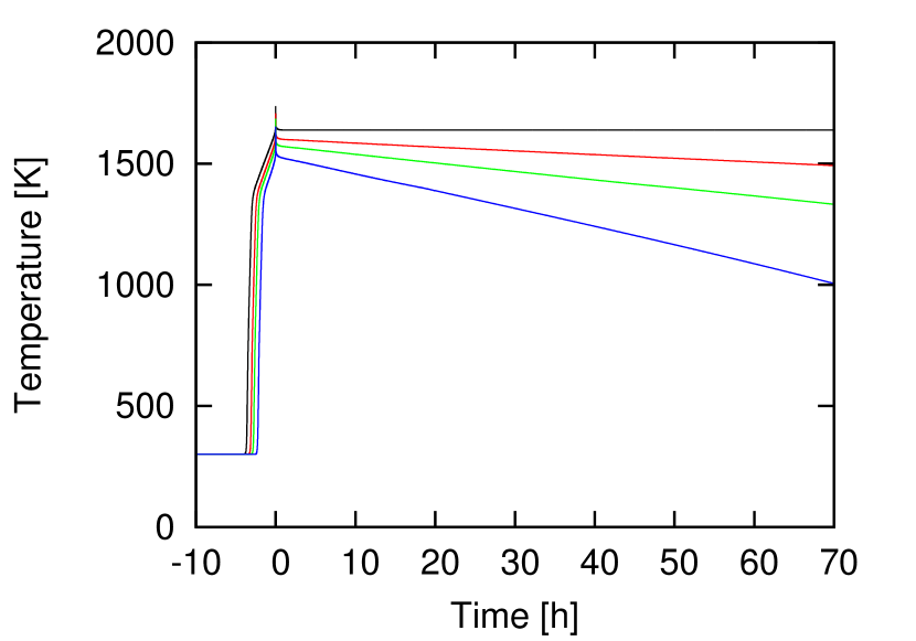
Figure 8: The standard shock (black) compared to simulations with a vertical energy loss with different loss parameters $L$ of 4 % (red), 2 % (green) and 1 % (blue) of the pressure scale height $H_{\mathrm{P}}=0.1$ AU at 3 AU. The shock speed is 6.5 km/s in all cases.

We have done this for different length scale parameters essentially simulating disks in which all the dust has settled into a very thin midplane layer. The results are compared to the standard case, which corresponds to $L=\infty$, in figure 8. As seen here, the higher the energy loss (the lower the length scale $L$), the smaller are the pre-shock regions and the peak temperatures. The length scale parameters chosen here are extremely small, only a few percent of the disk’s pressure scale height. It is very questionable if such disks exist. And even in those thin disks the particles are cooked at temperature above 1400 K for hours. The shock speed here is not even enough to completely melt the particles. With the vertical energy loss the particles still spend 2-3 hours in the high-temperature pre-shock phase. At higher shock speeds and therefore temperatures the situation is even worse.

3.3 Optically thin case

To investigate an optically thin case, where the particles can freely lose energy by radiation, we did another run where we set the mean intensity to $J_{\mathrm{rad}}\left(\tau\right)=\frac{\sigma}{\pi}T_{\mathrm{pre}}^{4}$ at every position. This means the gas and the particles are always in a radiation field with an ambient temperature of $T_{\mathrm{pre}}$. At the shock front the gas parameters are changed as usual and the particles can adapt to it. This could correspond for example to bow shocks created by planetesimals on eccentric orbits (Hood, 1998). Here we assume the shocked volume of the disk is small compared to the unshocked medium such that the particles mostly see the radiation field from the unshocked gas. Of course, this assumption breaks down close to the shock front, where fully three-dimensional calculations are needed. But it could also represent the case for which the shock loses all opacity due to dust evaporation.

Figure 9: Particle temperature of an optically thin shock with a shock speed of $V_{\mathrm{shock}}=9.0$ km/s. See text for details.

The result is shown in figure 9. As expected there is no pre-heating. Therefore the destination temperature for the jump conditions is lower and therefore also the target temperature. To reach the melting temperature in an optically thin case, we needed to increase the shock speed to $V_{\mathrm{shock}}=9.0$ km/s, instead of $\sim 7.0$ km/s in the optically thick cases.

Right after the shock the gas and particles cool down rapidly and approach asymptotically the ambient temperature. The particles are only for a few minutes at critical temperatures and are back below 500 K after $\sim 2$ h.

Figure 10: Cooling rates at $\mathrm{T}>1500~{}\mathrm{K}$ in the optically thin simulation (solid line) and with the Planck-mean opacity decreased by a factor of 10^-3 (dashed line). The discontinuity at $\sim 1820~{}\mathrm{K}$ is due to the change of the heat capacity regime introduced earlier in section 3.

Unfortunately, the cooling rates (figure 10, solid line) are at least two orders of magnitude too high in the crystallization regime at T $>1500$ K to produce the observed chondrule textures (see e.g. Hewins et al., 2005; Desch et al., 2012). Since the Planck mean opacity is always an upper limit on the opacity we arbitrarily decreased it by a factor of $10^{-3}$ to investigate the effect of lower opacities. The gas has then a lower ability to directly cool by radiation. The major cooling channel is then by thermal contact with the particles, which slows down the overall cooling process. The result is shown in figure 10 (dashed line). The cooling rates are still too large to be consistent with chondrule formation. Decreasing the opacity even further does not have any effect, since it is already low enough that the cooling via the particles is the dominant process.

In the bow shock scenario the optically thin approximation breaks down close to the shock front. Therefore, in reality there will be a pre-heating just before the shock front and less cooling after the shock. Whether this can produce the desired cooling rates has to be investigated by fully two-dimensional simulations. Further – but still one-dimensional – simulations by Morris et al. (2012) suggest that this could be the case.

4 Conclusions

Our 1-D radiative nebular shock model treats the variables at the downstream boundary as output of the model instead of boundary conditions that can be set. The iteration of the model then automatically finds the right downstream state of the matter, given the upstream boundary conditions. We find that this procedure prevents a post-shock slow (few minutes) cooling process. Instead, after the temperature spike and super-rapid cooling right after the main shock, the temperatures stay virtually constant. Only at distances from the shock comparable to the scale height of the disk will the 1-D approximation break down and will sideways (i.e. upward and downward) cooling set in. In our model we mimic this with a simple sideways cooling term.

For cases where the shock structure is local, for instance the bow shock of a planetesimal (see Morris et al., 2012), the shock scenario for chondrules might work because then the 1-D plane parallel assumption breaks down and sideways cooling can commence in a matter of hours. If the disk is optically thin then the cooling rates are too high to be consistent with the constraints on chondrule formation.

We conclude that while the nebular shock model for chondrules may work for local shocks (e.g. planetesimal bow shocks) the scenario has difficulties for global shocks in an optically thick nebula. This is because such global radiative shocks do not produce sufficient cooling after the temperature spike to be consistent with meteoritic constrains.

5 Acknowledgements

This work has been supported by the Deutsche Forschungsgemeinschaft Schwerpunktprogramm (DFG SPP) 1385 “The first ten million years of the solar system”.

We would like to thank Guy Libourel and an unknown referee for their fruitful comments on this paper.

Appendix A Drag force/frictional heating

If the particles are in a gas flow, which has a different velocity, they are accelerated or decellerated, respectively, by exchanging momentum with the gas. During this process they also get heated up by frictional heating of the gas molecules, just like a spacecraft is heated up while re-entering the Earth’s atmosphere. This was described by Gombosi et al. (1986, and references therein). If the particle radius is smaller than the mean free path of the gas molecules – which is valid up to a gas mass density of the order of $10^{-7}$ g/cm³ for millimeter-sized particles (Desch and Connolly, 2002) – the drag coefficient $C_{\mathrm{D}}$ used in equation (14) is given by

$$\begin{split}C_{\mathrm{D},j}=&\frac{2}{3s}\sqrt{\frac{\pi T_{j}}{T_{\mathrm{g}}}}+\frac{2s^{2}+1}{\sqrt{\pi}s^{3}}\exp\left(-s^{2}\right)\\ &+\frac{4s^{4}+4s^{2}-1}{2s^{4}}\mathrm{erf}\left(s\right).\end{split}$$ (33)

The parameter $s$ is the absolute value of the difference of the particle and the gas velocity measured in units of sound speeds

$$s=\frac{\left|V_{j}-V_{\mathrm{g}}\right|}{\sqrt{2k_{\mathrm{B}}T_{\mathrm{g}}/\overline{m}}},$$ (34)

with the mean molecular weight $\overline{m}$. The error function is defined as

$$\mathrm{erf}\left(x\right)=\frac{2}{\sqrt{\pi}}\int\limits_{0}^{x}e^{t^{2}}\mathrm{d}t.$$ (35)

The recovery temperature used in equation (18) is given by

$$\begin{split}T_{\mathrm{rec}}=&T_{\mathrm{g}}\frac{\gamma-1}{\gamma+1}\left[\frac{2\gamma}{\gamma-1}2s^{2}-\frac{1}{2}\right.\\ +&\left.\frac{2}{\sqrt{\pi}}\exp\left(-s^{2}\right)\mathrm{erf}^{-1}\left(s\right)\right]^{-1}.\end{split}$$ (36)

If $s\rightarrow 0$, which means particles and gas share the same velocity, then $T_{\mathrm{rec}}\rightarrow T_{\mathrm{g}}$, which means the particles adapt the gas temperature with time. The heat transfer coefficient $C_{\mathrm{H}}$ is given by

$$\begin{split}C_{\mathrm{H},j}=&\frac{\gamma+1}{\gamma-1}\frac{k_{\mathrm{B}}}{8\overline{m}s^{2}}\times\\ &\times\left[\frac{s}{\sqrt{\pi}}\exp\left(-s^{2}\right)+\left(\frac{1}{2}+s^{2}\right)\mathrm{erf}\left(s\right)\right].\end{split}$$ (37)

Appendix B Hydrodynamic calculations

Equations (27) and (29) have to be extensively manipulated to get to the two coupled differential equations (28) and (30) of the gas temperature and velocity. Since this calculus is somewhat obscure we want to present it here in all details.

Equation (27), which represents the momentum conservation consists of the derivative of three terms. We want to do the derivative for every term separately beginning with

$$\begin{split}&\frac{\partial}{\partial x}\sum\limits_{i=1}^{N_{I}}\rho_{i}V_{\mathrm{g}}^{2}=\frac{\partial}{\partial x}\sum\limits_{i=1}^{N_{I}}m_{i}n_{i}V_{\mathrm{g}}^{2}\\ &\quad=\sum\limits_{i=1}^{N_{I}}m_{i}V_{\mathrm{g}}\frac{\partial}{\partial x}\left(n_{i}V_{\mathrm{g}}\right)+\sum\limits_{i=1}^{N_{I}}m_{i}n_{i}V_{\mathrm{g}}\frac{\partial}{\partial x}V_{\mathrm{g}}.\end{split}$$ (38)

The first term here can be replaced using the continuity equation of the gas (24) while the second term is already in the needed form only replacing the sum with the total gas mass density

$$\begin{split}&\frac{\partial}{\partial x}\sum\limits_{i=1}^{N_{I}}\rho_{i}V_{\mathrm{g}}^{2}=V_{\mathrm{g}}\sum\limits_{i=1}^{N_{I}}\sum\limits_{k=0}^{N_{K}}m_{i}R_{i,k}+\rho_{\mathrm{g}}V_{\mathrm{g}}\frac{\partial}{\partial x}V_{\mathrm{g}}.\end{split}$$ (39)

Similar transformations can be applied to the second term of equation (27)

$$\begin{split}&\frac{\partial}{\partial x}\sum\limits_{i=1}^{N_{I}}n_{i}k_{\mathrm{B}}T_{\mathrm{g}}\\ &\quad=k_{\mathrm{B}}T_{\mathrm{g}}\sum\limits_{i=1}^{N_{I}}\frac{\partial}{\partial x}n_{i}+k_{\mathrm{B}}\sum\limits_{i=1}^{N_{I}}n_{i}\frac{\partial}{\partial x}T_{\mathrm{g}}.\end{split}$$ (40)

As with equation (38) the continuity equation of the gas (24) can be used to manipulate the first term, while the second is already in its final form

$$\begin{split}&\frac{\partial}{\partial x}\sum\limits_{i=1}^{N_{I}}n_{i}k_{\mathrm{B}}T_{\mathrm{g}}\\ \quad=&\frac{k_{\mathrm{B}}T_{\mathrm{g}}}{V_{\mathrm{g}}}\sum\limits_{i=1}^{N_{I}}\left(\sum\limits_{k=0}^{N_{K}}R_{i,k}-n_{i}\frac{\partial}{\partial x}V_{\mathrm{g}}\right)\\ &+k_{\mathrm{B}}\sum\limits_{i=1}^{N_{I}}n_{i}\frac{\partial}{\partial x}T_{\mathrm{g}}.\end{split}$$ (41)

The third term of equation (27) with the particle momentum can be transformed as

$$\begin{split}&\frac{\partial}{\partial x}\sum\limits_{j=1}^{J}n_{j}m_{j}V_{j}^{2}\\ &\quad=\sum\limits_{j=1}^{N_{J}}m_{j}V_{j}\frac{\partial}{\partial x}\left(n_{j}V_{j}\right)+\sum\limits_{j=1}^{N_{J}}n_{j}m_{j}V_{j}\frac{\partial}{\partial x}V_{j}\\ &\quad+\sum\limits_{j=1}^{N_{J}}n_{j}V_{j}^{2}\frac{\partial}{\partial x}m_{j}.\end{split}$$ (42)

The first term is equal to zero because of the continuity equation of the particles (13) and the second term can be replaced by the drag force (17). The change in mass in the third term can be transformed to a change in particle radius

$$\begin{split}&\frac{\partial}{\partial x}\sum\limits_{j=1}^{N_{J}}n_{j}m_{j}V_{j}^{2}\\ &\quad=\sum\limits_{j=1}^{N_{J}}n_{j}F_{\mathrm{drag},j}+\sum\limits_{j=1}^{N_{J}}n_{j}V_{j}^{2}4\pi a_{j}^{2}\rho_{j}\frac{\partial}{\partial x}a_{j}.\end{split}$$ (43)

Adding all terms up this leads to equation (28).

Similar transformations can be applied to equation (29). We do them here for all terms in the sums separately. The first term in the sum over $i$ represents the kinetic energy of the gas due to its flow

$$\begin{split}&\frac{\partial}{\partial x}\sum\limits_{i=1}^{N_{I}}\frac{1}{2}n_{i}m_{i}V_{\mathrm{g}}^{3}\\ &=\frac{1}{2}V_{\mathrm{g}}^{2}\sum\limits_{i=1}^{N_{I}}m_{i}\frac{\partial}{\partial x}\left(n_{i}V_{\mathrm{g}}\right)+V_{\mathrm{g}}^{2}\sum\limits_{i=1}^{I}m_{i}n_{i}\frac{\partial}{\partial x}V_{\mathrm{g}}.\end{split}$$ (44)

While the second term of this result is already in its final form, the first term can be replaced by the continuity equation of the gas (24)

$$\begin{split}&\frac{\partial}{\partial x}\sum\limits_{i=1}^{N_{I}}\frac{1}{2}n_{i}m_{i}V_{\mathrm{g}}^{3}\\ &=\frac{1}{2}V_{\mathrm{g}}^{2}\sum\limits_{i=1}^{N_{I}}\sum\limits_{k=0}^{N_{K}}m_{i}R_{i,k}+V_{\mathrm{g}}^{2}\sum\limits_{i=1}^{N_{I}}m_{i}n_{i}\frac{\partial}{\partial x}V_{\mathrm{g}}.\end{split}$$ (45)

The second term in the sum over $i$ in equation (29) is the combined internal energy of the gas and the pressure. It can be transformed as follows

$$\begin{split}&\frac{\partial}{\partial x}\sum\limits_{i=1}^{N_{I}}n_{i}V_{\mathrm{g}}\frac{f_{i}+2}{2}k_{\mathrm{B}}T_{\mathrm{g}}\\ &=k_{\mathrm{B}}T_{\mathrm{g}}\sum\limits_{i=1}^{N_{I}}\frac{f_{i}+2}{2}\frac{\partial}{\partial x}\left(n_{i}V_{\mathrm{g}}\right)\\ &\quad+k_{\mathrm{B}}V_{\mathrm{g}}\sum\limits_{i=1}^{N_{I}}n_{i}\frac{f_{i}+2}{2}\frac{\partial}{\partial x}T_{\mathrm{g}}\\ &=k_{\mathrm{B}}T_{\mathrm{g}}\sum\limits_{i=1}^{N_{I}}\sum\limits_{i=0}^{N_{K}}\frac{f_{i}+2}{2}R_{i,k}\\ &\quad+k_{\mathrm{B}}V_{\mathrm{g}}\sum\limits_{i=1}^{N_{I}}n_{i}\frac{f_{i}+2}{2}\frac{\partial}{\partial x}T_{\mathrm{g}},\end{split}$$ (46)

where again the continuity equation of the gas (24) was used.

The first term in the sum over $j$ in equation (29) – the kinetic energy of the particles – can be written as

$$\begin{split}&\frac{1}{2}\frac{\partial}{\partial x}\sum\limits_{j=1}^{N_{J}}n_{j}m_{j}V_{j}^{3}\\ &=\frac{1}{2}\sum\limits_{j=1}^{N_{J}}m_{j}V_{j}^{2}\frac{\partial}{\partial x}\left(n_{j}V_{j}\right)+\sum\limits_{j=1}^{N_{J}}n_{j}m_{j}V_{j}^{2}\frac{\partial}{\partial x}V_{j}\\ &\quad+\frac{1}{2}\sum\limits_{j=1}^{N_{J}}n_{j}V_{j}^{3}\frac{\partial}{\partial x}m_{j}.\end{split}$$ (47)

The first term here is again equal to zero because of equation (13). The second term can be replaced by the drag force (17), while the third term can again be transformed into a derivative of the particle radius

$$\begin{split}&\frac{1}{2}\frac{\partial}{\partial x}\sum\limits_{j=1}^{N_{J}}n_{j}m_{j}V_{j}^{3}\\ &=\sum\limits_{j=1}^{N_{J}}n_{j}V_{j}F_{\mathrm{drag},j}+2\pi\sum\limits_{j=1}^{N_{J}}n_{j}V_{j}^{3}a_{j}^{2}\rho_{j}\frac{\partial}{\partial x}a_{j}.\end{split}$$ (48)

The second term in the sum over $j$ in equation (29) is the internal energy of the particles

$$\begin{split}&\frac{\partial}{\partial x}\sum\limits_{j=1}^{N_{J}}n_{j}V_{j}m_{j}C_{\mathrm{P},j}T_{j}\\ &=\sum\limits_{j=1}^{N_{J}}m_{j}C_{\mathrm{P},j}T_{j}\frac{\partial}{\partial x}\left(n_{j}V_{j}\right)\\ &\quad+\sum\limits_{j=1}^{N_{J}}n_{j}V_{j}\frac{\partial}{\partial x}\left(m_{j}C_{\mathrm{P},j}T_{j}\right)\\ &=\sum\limits_{j=1}^{N_{J}}n_{j}V_{j}\frac{\partial}{\partial x}\left(m_{j}C_{\mathrm{P},j}T_{j}\right),\end{split}$$ (49)

where again the continuity equation of the particles (13) was used. The remaining term can be further transformed to

$$\begin{split}&\frac{\partial}{\partial x}\sum\limits_{j=1}^{N_{J}}n_{j}V_{j}m_{j}C_{\mathrm{P},j}T_{j}\\ &=\sum\limits_{j=1}^{N_{J}}n_{j}V_{j}m_{j}C_{\mathrm{P},j}\frac{\partial}{\partial x}T_{j}\\ &\quad+4\pi\sum\limits_{j=1}^{N_{J}}n_{j}V_{j}C_{\mathrm{P},j}T_{j}a_{j}^{2}\rho_{j}\frac{\partial}{\partial x}a_{j}.\end{split}$$ (50)

The derivative of the radiative flux $F_{\mathrm{rad}}$ is already given in equation (9). Summing up every term, this yields equation (30). The formulas for $\frac{\partial}{\partial x}T_{j}$ and $\frac{\partial}{\partial x}a_{j}$ can be inserted from equations (20) and (22). Equations (28) and (30) are two coupled differential equations of the form

$$\begin{split}A\frac{\partial}{\partial x}V_{\mathrm{g}}+B\frac{\partial}{\partial x}T_{\mathrm{g}}&=C\\ D\frac{\partial}{\partial x}V_{\mathrm{g}}+E\frac{\partial}{\partial x}T_{\mathrm{g}}&=F,\end{split}$$

with the respective $A,\ B,\ C,\ D,\ E$ and $F$. Decoupled they can be written as

$$\begin{split}\frac{\partial}{\partial x}V_{\mathrm{g}}&=\frac{CE-BF}{AE-BD}\\ \frac{\partial}{\partial x}T_{\mathrm{g}}&=\frac{AF-CD}{AE-BD}.\end{split}$$

References

- Bell et al. (1997) Bell, K. R., Cassen, P. M., Klahr, H. H., Henning, T., 1997. The Structure and Appearance of Protostellar Accretion Disks: Limits on Disk Flaring. The Astrophysical Journal 486, 372 – 387.
- Boley and Durisen (2008) Boley, A. C., Durisen, R. H., 2008. Gravitational Instabilities, Chondrule Formation, and the FU Orionis Phenomenon. The Astrophysical Journal 685, 1193 – 1209.
- Boss (1996) Boss, A. P., 1996. A concise guide to chondrule formation models. In: Chondrules and the Protoplanetary Disk. Cambridge University Press, pp. 257 – 263.
- Brown et al. (1989) Brown, P. N., Byrne, G. D., Hindmarsh, A. C., 1989. VODE: A variable-coefficient ODE Solver. SIAM Journal on Scientific Computing 10, 1038–1051.
- Cherchneff et al. (1992) Cherchneff, I., Barker, J. R., Tielens, A. G. G. M., 1992. Polycyclic aromatic hydrocarbon formation in carbon-rich stellar envelopes. The Astrophysical Journal 401, 269 – 281.
- Ciesla (2005) Ciesla, F. J., 2005. Chondrule-forming processes – An Overview. In: Chondrites and the Protoplanetary Disk. Astronomical Society of the Pacific, p. 811.
- Ciesla and Hood (2002) Ciesla, F. J., Hood, L. L., 2002. The Nebular Shock Wave Model for Chondrule Formation: Shock Processing in a Particle-Gas Suspension. Icarus 158, 281 – 293.
- Desch and Connolly (2002) Desch, S. J., Connolly, Jr., H. C., 2002. A model of the thermal processing of particles in solar nebular shocks: Application to the cooling rates of chondrules. Meteorites & Planetary Science 37, 183–207.
- Desch et al. (2012) Desch, S. J., Morris, M. A., Connolly, Jr., H. C., Boss, A. P., 2012. The importance of experiments: Constraints on chondrule formation models. Meteorites & Planetary Science 47, 1139 – 1156.
- Fedkin et al. (2012) Fedkin, A. V., Grossman, L., Ciesla, F. J., Simon, S. B., 2012. Mineralogical and isotopic constraints on chondrule formation from shock wave thermal histories. Geochimica et Cosmochimica Acta 87, 81 – 116.
- Gombosi et al. (1986) Gombosi, T. I., Nagy, A. F., Cravens, T. W., 1986. Dust and neutral gas modeling of the inner atmospheres of comets. Reviews of Geophysics.
- Hewins et al. (2005) Hewins, R. H., Connolly, H. C., Lofgren, G. E., J., Libourel, G., 2005. Experimental Constraints on Chondrule Formation. In: Chondrites and the Protoplanetary Disk. Vol. 341. ASP Conference Series, p. 286.
- Hood (1998) Hood, L. L., 1998. Thermal processing of chondrule precursors in planetesimal bow shocks. Meteoritics & Planetary Science 33, 97 – 107.
- Hood and Horanyi (1991) Hood, L. L., Horanyi, M., 1991. Gas dynamic heating of chondrule precursor grains in the solar nebula. Icarus 93, 259 – 269.
- Iida et al. (2001) Iida, A., Nakamoto, T., Susa, H., Nakagawa, Y., 2001. A Shock Heating Model for Chondrule Formation in a Protoplanetary Disk. Icarus 153, 130 – 150.
- Kley and Nelson (2012) Kley, W., Nelson, R. P., 2012. Planet-Disk Interaction and Orbital Evolution. Annual Review of Astronomy and Astrophysics 50, 211–249.
- Mihalas and Weibel-Mihalas (1999) Mihalas, D., Weibel-Mihalas, B., 1999. Foundations of Radiation Hydrodynamics. Dover.
- Morris et al. (2012) Morris, M. A., Boley, A. C., Desch, S. J., Athanassiadou, T., 2012. Chondrule formation in bow shocks around eccentric planetary embryos. The Astrophysical Journal 752.
- Morris and Desch (2010) Morris, M. A., Desch, S. J., 2010. Thermal Histories of Chondrules in Solar Nebula Shocks. The Astrophysical Journal 722, 1474 – 1494.
- Semenov et al. (2003) Semenov, D., Henning, T., Helling, C., Ilgner, M., Sedlmayr, E., 2003. Rosseland and Planck mean opacities for protoplanetary discs. Astronomy & Astrophysics 410, 611–621.
- Villeneuve et al. (2009) Villeneuve, J., Chaussidon, M., Libourel, G., 2009. Homogeneous Distribution of 26Al in the Solar System from the Mg Isotopic Composition of Chondrules. Science 325, 985 – 988.
- Yu et al. (1996) Yu, Y., Hewins, H. H., Zanda, B., 1996. Sodium und Sulfur in Chondrules: Heating Time and Cooling Curves. In: Chondrules and the Protoplanetary Disk. Cambridge University Press, pp. 213 – 219.