Maser and Infrared Studies of Oxygen-Rich Late/Post-AGB Stars and Water Fountains: Development of a New Identification Method

Abstract

We explored an efficient method to identify evolved stars with oxygen-rich envelopes in the late AGB or post-AGB phase of stellar evolution, which include a rare class of objects — the “water fountains”. Our method considers the OH and H₂O maser spectra, the near infrared $Q$-parameters (these are colour indices accounting for the effect of extinction), and far-infrared AKARI colours. Here we first present the results of a new survey on OH and H₂O masers. There were 108 colour-selected objects: 53 of them were observed in the three OH maser lines (1612, 1665, and 1667 MHz), with 24 detections (16 new for 1612 MHz); and 106 of them were observed in the H₂O maser line (22 GHz) with 24 detections (12 new). We identify a new potential water fountain source, IRAS 19356$+$0754, with large velocity coverages of both OH and H₂O maser emission. In addition, several objects with high velocity OH maser emission are reported for the first time. The $Q$-parameters as well as the infrared [09]$-$[18] and [18]$-$[65] AKARI colours of the surveyed objects are then calculated. We suggest that these infrared properties are effective in isolating aspherical from spherical objects, but the morphology may not necessarily be related to the evolutionary status. Nonetheless, by considering altogether the maser and infrared properties, the efficiency of identifying oxygen-rich late/post-AGB stars could be improved.

1 Introduction

The post asymptotic giant branch (post-AGB) phase is a short transition phase for intermediate-mass stars (about 1 to 8 $M_{\odot}$) in the course of stellar evolution. It comes after the mass-losing AGB phase that creates thick circumstellar envelopes, and before the planetary nebula (PN) phase in which those envelopes are ionized by radiation from exposed hot central stars and interstellar ultraviolet emission (see, Van Winckel, 2003, for a review). The duration of the post-AGB phase could be just $\sim$30 years in case of a relatively massive star (i.e. close to 8 $M_{\odot}$), or up to $\sim$$5\times 10^{4}$ years for a lower mass star (Blöcker, 1995). Post-AGB stars are often invisible in the optical wavelength range due to their low envelope temperature ($\leq$200 K). They are usually observable at longer wavelengths because radiation from the stellar photosphere is absorbed and re-emitted by the thick envelope. As opposed to usual AGB stars, most of the post-AGB stars are surrounded by circumstellar shells with aspherical morphology, showing bipolar or even multipolar structures in high resolution infrared images (e.g., Lagadec et al., 2011). Sahai & Trauger (1998) suggested that high velocity jets will form at the late AGB or early post-AGB phase which may affect the morphologies of the remnants of the formerly ejected, approximately spherical shells. Studying objects with such jets is therefore an essential part in understanding the evolutionary process of post-AGB stars.

There are still no fully established theories on jet formation in AGB and post-AGB stars. One of the suggested scenarios depicts a binary system that consists of a star with a thick envelope and its low-mass ($<$0.3 $M_{\odot}$) companion (Nordhaus & Blackman, 2006; Huggins, 2007). A torus is firstly formed due to equatorially enhanced mass-loss. The jet is launched after that phase. The launching jet power might come from the magnetocentrifugal force, as is the case of young stellar objects (e.g, Frank & Blackman, 2004). For oxygen-rich stars (i.e. intermediate-mass evolved stars with more oxygen than carbon atoms), there is a class of objects called the “water fountains (WFs)” which exhibit a special type of jets: the small in scale ($<$1000 AU), high velocity ($\geq 50$ km s^-1), and strongly collimated bipolar jets. The name comes from the fact that those jets can be traced by H₂O maser emission. From the point of view of spectroscopy, an object is proposed to be a WF if its H₂O maser emission spectrum shows a larger velocity coverage than that of its 1612 MHz OH maser (see Imai, 2007; Desmurs, 2012, for a WF review). It is because the typical OH double-peaked line shape reveals the terminal expansion velocity (normally $\leq$25 km s^-1) of the spherically expanding envelope formed by the AGB mass-loss. A larger spectral coverage of H₂O will therefore imply an outflow with velocity exceeding that of the spherical envelope. It is confirmed by high-angular-resolution interferometric observations of the 22 GHz H₂O maser line that this phenomenon is caused by the existence of high velocity bipolar jets (e.g., Imai et al., 2002; Yung et al., 2011). Most of the WF H₂O maser spectra have a velocity coverage larger than 50 km s^-1, reaching up to 200–300 km s^-1. WFs are often regarded as objects which have just started to depart from spherical symmetry. For this reason, WFs are commonly seen as young post-AGB stars (e.g, Suárez et al., 2008; Walsh et al., 2009; Desmurs, 2012). In addition to WFs, some OH objects (without H₂O maser detections) are found to have bipolar jets as well (Zijlstra et al., 2001). These objects usually show rather irregular OH maser profiles with large velocity coverages (about 30–80 km s^-1). The irregular profiles imply that these objects are more evolved than usual AGB stars (Deacon et al., 2004). However, there are also exceptional cases of AGB stars with aspherical structures: W 43A (Imai et al., 2002), X Her (Hirano et al., 2004), and V Hya (Nakashima, 2005) are examples of AGB stars with bipolar jets.

Even though the exact evolutionary phase for the jet to be launched is uncertain, it is clear from the above studies that jets play an important role in changing the morphology of envelopes at later stages of stellar evolution. In order to understand the underlying process of such shaping mechanism, we need to obtain a larger sample of late AGB/post-AGB stars, especially those associated with high velocity jets such as the WFs. In our previous H₂O maser survey (Yung et al., 2013, hereafter Paper I), we have shown that the AKARI two-colour diagram could be useful in selecting AGB and post-AGB star candidates, providing an alternative way of object selection besides the well-known IRAS two-colour diagram (van der Veen & Habing, 1988) that has been used in many major surveys (see Paper I for a summary of surveys). We have found four candidates of “low-velocity” WFs, which are objects that have a small H₂O maser velocity coverage ($\sim$30 km s^-1), but still fulfill the other WF criteria (i.e., the H₂O coverage is larger than that of OH, and the IRAS colours are very red). These could be immature WFs, but their true status has to be confirmed by observations with high angular resolution, e.g., very long baseline interferometric observations of maser lines, or infrared imagings with adaptive optics.

In this paper, we further explore potentially reliable indicators for the evolutionary status of evolved stars, in particular for those at the late AGB/post-AGB phase. We have selected $\sim$100 evolved star candidates in the late AGB/post-AGB phase by using the AKARI colour criteria suggested in Paper I. Then, we searched for the OH and H₂O maser emission from these objects because those maser lines can be a probe of high velocity jets. Finally, we study the object distribution on the $Q1$–$Q2$ diagram (which is an extinction-free infrared tool proposed by Messineo et al., 2012, see Section 4.1) and also the AKARI two-colour diagram. The former reflects the near-infrared properties of the objects, while the latter is predominantly affected by the far-infrared emission. Observational details of this work including the source selection are given in Section 2; the results are presented in Section 3, followed by the discussion in Section 4. Main conclusions are summarized in Section 5.

2 Object Selection and Maser Observations

2.1 Object Selection

Table 1 displays parameters of the 108 objects observed in this project. Most of the objects were selected from the AKARI Point Source Catalogue (Kataza et al., 2010; Yamamura et al., 2010), according to their [09]$-$[18] and [18]$-$[65] colours. In Paper I, we have defined the empirical “post-AGB star” colour region by $0.5\leq[09]$$-$$[18]\leq 4.5$ and $-0.5\leq[18]$$-$$[65]\leq 2$, where $[m]$$-$$[n]$=$2.5\log(F_{n}/F_{m})$, with $F_{m}$ and $F_{n}$ representing the band fluxes at $m$ and $n$ $\mu$m, respectively. However, this region still suffers from contamination by young stellar objects (YSOs). Therefore, we have also checked the mid-infrared images of all the objects during the selection, in order to exclude obvious YSO candidates. Evolved stars usually appear as point sources in mid-infrared images, e.g., in images taken with the Midcourse Space Experiment (MSX) and Wide-field Infrared Survey Explorer (WISE). On the contrary, YSOs are often embedded in comparatively large scale nebulosities which show extended emission features at mid-infrared wavelengths. In addition to these new objects which were not observed before in the 1612 MHz OH nor in the 22 GHz H₂O maser lines, some known H₂O maser sources (especially those newly reported in Paper I) with no reported OH maser counterparts were included. We have also re-visited a few known WFs and low-velocity WF candidates. The declinations of the targets are limited to $\delta>-25^{\circ}$ because of the telescope location. Owing to limited observing time, not all objects were observed in both lines (see Table 1).

2.2 Maser Observations and Data Reduction

The OH and H₂O maser observations were carried out with the Effelsberg 100 m radio telescope from 2012 October 11 to 18. For the OH observations, an 1.3–1.7 GHz HEMT receiver was used with a Fast-Fourier-Transform (FFT) spectrometer as backend. The frequency coverage of the spectrometer was 100 MHz. The central frequency was set to 1640.0 MHz so that three of the four ${}^{2}\Pi_{3/2}$ $J=3/2$, 18 cm $\Lambda$-doublet lines were covered. The adopted rest frequencies of the OH lines were 1612.2310 MHz for the satellite line, and 1665.4018, 1667.3590 MHz for the two main lines (Lovas, 2004). The FWHM of the beam was about 8′. With 32,768 spectral channels, the corresponding channel spacing for the three target frequencies was between 0.5 km s^-1 and 0.6 km s^-1. For the H₂O observation, an 18–26 GHz HEMT receiver was used with another FFT spectrometer. The frequency coverage of the spectrometer was 500 MHz, and the central frequency was set to 22.235080 GHz, the rest frequency of the $6_{16}\rightarrow 5_{23}$ transition line of H₂O (Lovas, 2004). The FWHM of the beam was about 40″. The number of spectral channels was again 32,768, so the channel spacing was about 0.8 km s^-1. Velocity resolutions are coarser than the channel spacing, by 16%. The scale of the local-standard-of-rest velocity ($V_{\rm LSR}$) for both OH and H₂O observations has been confirmed to be accurate by comparisons with spectra from known sources.

An ON/OFF cycle of 2 minutes was used in a position-switching mode. For OH masers, the OFF-position was 1^∘ west in azimuth from the ON-position. For H₂O masers, the OFF-position was set to $-75$ s with respect to the ON-position along right ascension. This option was chosen because it kept the OFF-position exactly on the same track as the ON-position. The observing time for each source was about 6–20 minutes, with the exception of IRAS 19356$+$0754, which was observed for 6 hours. The long integration time was needed to confirm the weak line components from this object (see Section 3.2). The root-mean-square (rms) noise level ranges from 0.001 to 0.1 Jy for both OH and H₂O maser observations. Pointing was calibrated every 2–3 hours by doing 2-points cross scans on bright quasars with strong continuum emission. The typical pointing accuracy is about 5″. Flux calibration was obtained using pointing sources with known flux densities (see, Ott et al., 1994).

Data reduction were performed with the Continuum and Line Analysis Single-dish Software (CLASS) package. Individual scans on each object were inspected by eye, and those with obvious artifacts were discarded. The remaining scans were then averaged. The baseline of each spectrum was fit by a low order (1st–3rd) polynomial and subtracted, using channels free of emission features.

3 Results

3.1 Overview of the OH and H₂O Maser Detections

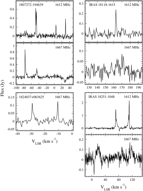
Figure 1: Spectra of objects with OH maser detections only.

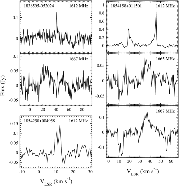
Figure 1: Continued

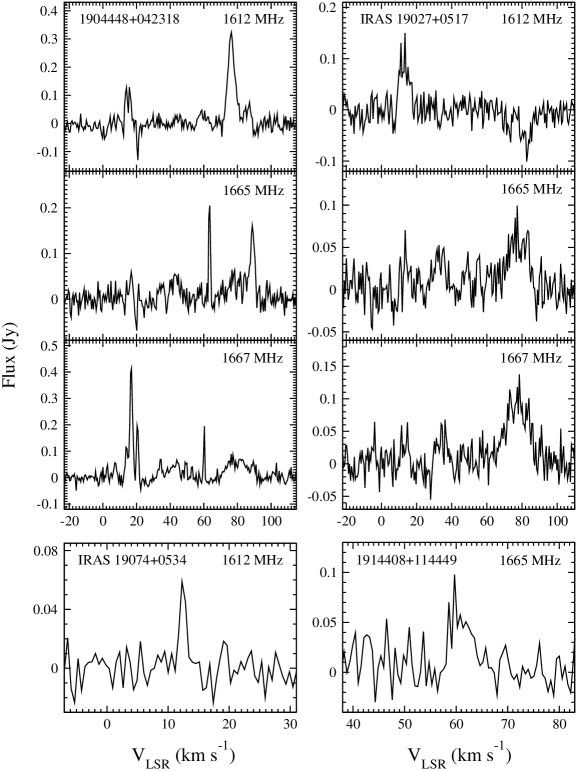
Figure 1: Continued

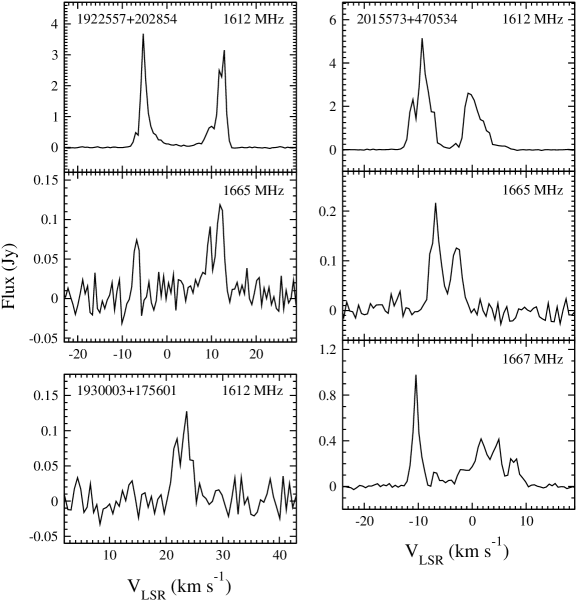
Figure 1: Continued

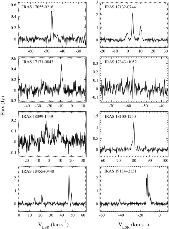
Figure 2: Spectra of objects with H₂O maser detections only.

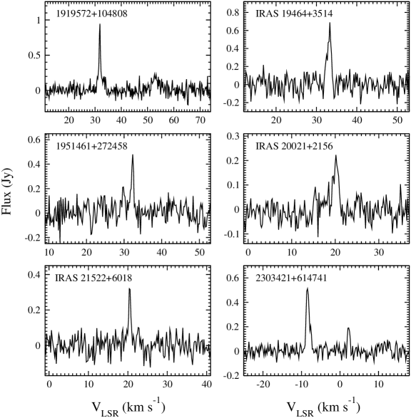
Figure 2: Continued

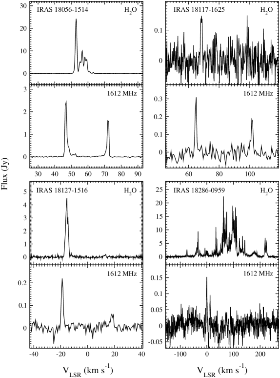
Figure 3: Spectra of objects with both OH and H₂O maser detections.

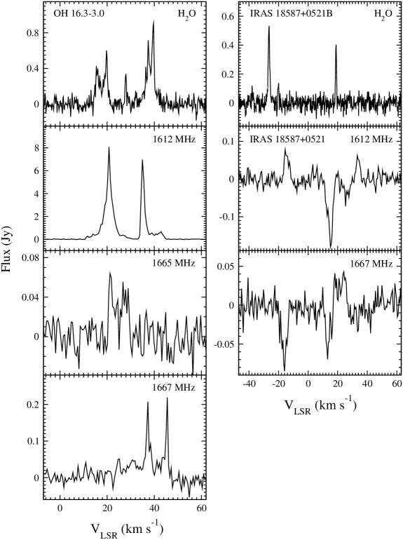
Figure 3: Continued

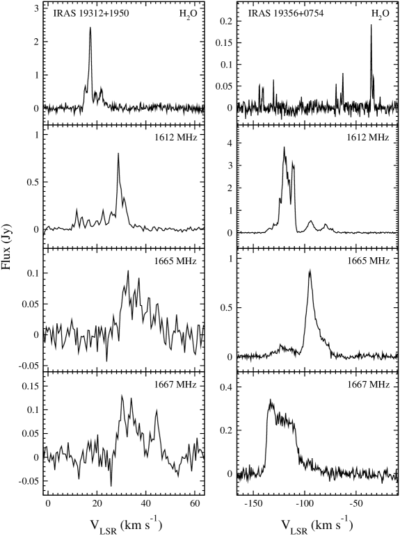
Figure 3: Continued

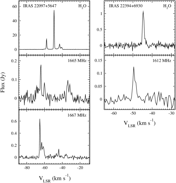
Figure 3: Continued

Figure 1 shows the spectra for objects only with OH maser detections, while Figure 2 is for H₂O masers only. For objects with both OH and H₂O masers detected, their velocity-aligned spectra are shown in Figure 3. Table 1 summarizes the coordinates and infrared colours of the objects that have OH and/or H₂O detections. The corresponding spectral parameters of all the detections and non-detections are presented in Tables 2 to 5. Amongst 108 selected objects, 53 were observed in OH (which includes the 1612, 1665, and 1667 MHz maser lines), with 24 detections. There are 16 new 1612 MHz, 9 new 1665 MHz, and 11 new 1667 MHz detections. Some of these newly detected lines originate from the the same objects where previously other OH maser lines have already been reported. For the H₂O maser line at 22 GHz, 106 objects were observed with 24 detections (12 new). The detection rates of both OH and H₂O masers agree with some previous maser surveys on post-AGB stars (see Habing, 1996, for a discussion on the detection rates) , e.g., $\sim$40% for OH masers (te Lintel Hekkert & Chapman, 1996), and $\sim$25% for H₂O masers (Valdettaro et al., 2001; Deacon et al., 2007).

Similar to the results of previous surveys such as those of te Lintel Hekkert et al. (1989) and te Lintel Hekkert (1991), the majority of the OH spectra show a double-peaked profile at 1612 MHz (Figure 1). This is a common characteristic for Type II OH/IR stars which are classified by their IRAS colours: $-0.30<[12]$$-$$[25]<-0.08$ (Habing, 1996). The double-peaked emission profile features two 1612 MHz peaks that reveal the line-of-sight velocities of the approaching and receding sides of the spherically expanding envelope. The velocity halfway between the peaks is taken as the systemic velocity of the star. The 1665 and 1667 MHz main lines usually show similar double-peak profiles, but in most cases they are fainter than those of the 1612 MHz satellite line. On the other hand, there are three objects in our observations with only the main lines detected, namely 1824037$+$063625, 1914408$+$114449, and IRAS 22097$+$5647. In particular, IRAS 22097$+$5647 belongs to the Type I OH/IR stars with $-0.45<[12]$$-$$[25]<-0.30$ (Habing, 1996). The OH emission profile from these stars usually shows only the main lines; occasionally the satellite line is also found but at a much weaker level. The profiles of the main lines usually have an irregular line shape, because the main lines originate from the accelerating region of an expanding envelope, where the gradient in the radial velocity produces the irregular line shape (Habing, 1996). We do not have enough information for 1824037$+$063625 and 1914408$+$114449; they could be evolved stars or YSOs. Nonetheless, they are point-sources in mid-infrared images, e.g., the 12 $\mu$m images from the WISE catalogue which have an angular resolution of $6\farcs 5$ (Wright et al., 2010), suggesting that there are no clear star forming activities around these objects. Absorption features are found in several spectra (see Figure 1 and Table 2), but they may be caused by foreground objects (e.g., te Lintel Hekkert & Chapman, 1996), or by some emission that contaminates the OFF-positions.

Most of the obtained H₂O maser spectra have a double-peaked (with some of them only showing a weak secondary feature) or an irregular profile (Figure 2). It is known that H₂O masers generally have three common emission profiles: single-peaked, double-peaked, and irregular (e.g., Takaba et al., 1994; Deacon et al., 2007). A single-peak at the systemic velocity is quite commonly found in AGB stars with a lower mass-loss rate in the case of a spherically expanding envelope, because the masers are mainly tangentially amplified. When the mass-loss rate increases as the star evolves, the profile will likely become double-peaked because maser amplification along the radial direction is now predominant, where the two peaks come from the approaching and receding sides of the spherical envelope (Takaba et al., 1994). However, the above justification is not necessarily true for all cases because maser line profiles are not solely governed by the mass-loss rate. An irregular profile is often seen in further evolved objects (e.g., the post-AGB star IRAS 15445$-$5449, Pérez-Sánchez et al., 2011) or YSOs (e.g., W51-IRS2, Morita et al., 1992) because of the development of irregular motions possibly induced by non-spherical (e.g., bipolar) outflow components. Note that the H₂O maser emission would have a similar or slightly smaller velocity coverage than the OH maser in most evolved stars with the notable exception of the WFs.

3.2 Notable Individual Objects

3.2.1 Water Fountains

IRAS 18286$-$0959. It is a known WF suggested to harbour an episodic precessing jet which produces a “double-helix” jet pattern (Yung et al., 2011). In paper I, we have already noticed that the H₂O maser velocity coverage of this object has increased from 220 km s^-1to 263 km s^-1 since its first detection (Deguchi et al., 2007). This time, more components were detected and the resulting coverage is now $\sim$350 km s^-1 (Figure 3). It is not certain whether the jet really accelerates, or whether it is simply due to maser flux variation so that the new components were not detected in previous observations. For the OH maser, this object was reported to have a single 1612 MHz feature at 39.5 km s^-1 (Sevenster et al., 2001). However, here we detected two close peaks at $-0.2$ km s^-1 and $12.3$ km s^-1. The 1612 MHz emission is usually stable on time scales of months or even longer. This is why the disappearance of the 39.5 km s^-1 peak and the detection of the new components are unexpected. The reason behind is unknown, but it might hint to the fact that the OH shell has been disturbed. Possibilities include the interference from a high velocity jet, or some turbulent motion due to the existence of a nearby object.

IRAS 19134$+$2131. The first detailed interferometric study of the H₂O masers from this WF was presented by Imai et al. (2007). Its H₂O maser spectrum used to have three peaks at about $-120$ km s^-1, $-40$ km s^-1, and $-10$ km s^-1. All of them were still detected in 2011 (Paper I). This time the most blueshifted peak (i.e. at $-120$ km s^-1) disappeared, and the remaining double-peak profile resembles those of normal AGB stars (Figure 2). There has been no OH maser detection toward this object. A longer exposure time may be needed.

IRAS 19356$+$0754. This object could be a new member of the WF class. Its OH 1612 MHz maser spectrum has many emission peaks with velocities ranging from $-138$ km s^-1 to $-71$ km s^-1. The large velocity coverage ($\sim$67 km s^-1) and the irregular profile are common for very evolved objects like post-AGB stars or proto-planetary nebulae (PPNe; Zijlstra et al., 2001). The 1665 and 1667 MHz lines also have an irregular profile and span a similar velocity range, but the total flux is smaller than that of the 1612 MHz line. The H₂O maser spectrum consists of multiple peaks with a total velocity coverage of about 119 km s^-1 (from $-145$ km s^-1to $-26$ km s^-1), larger than that of the OH masers. The H₂O lines are very weak: the strongest peak is only about 0.2 Jy. Note that this object was observed in H₂O before by Suárez et al. (2007), but at that time the result was a non-detection (corresponding rms $\sim 0.04$ Jy). Therefore, the maser emission could be at a minimum during their observing period, while another possibility is that the maser appeared after 2007. The systemic velocity of this object is about $-105$ km s^-1 according to the maser spectra. The kinematic distance derived using the systemic velocity and the Galactic rotation curve (Kothes & Dougherty, 2007) is about 30 kpc. This puts the object outside the Milky Way, which is unlikely true. The total infrared flux estimated from its SED is about $2.3\times 10^{-12}$ W m^-2. Assuming a luminosity of 10,000 $L_{\odot}$ (quite typical for a post-AGB star), the resultant luminosity distance is about 12 kpc, but this distance also includes a large uncertainty.

3.2.2 Objects with High Velocity OH Maser Emission

1807272$-$194639. The OH 1612 MHz spectrum shows four emission peaks (at about $-77$ km s^-1, $-48$ km s^-1, $4$ km s^-1, and $30$ km s^-1) with a maximum velocity coverage of $\sim$107 km s^-1 (Figure 1). A “U-shaped” double-peaked profile is found in the 1667 MHz spectrum, which is a signature of a spherically expanding envelope commonly associated with AGB stars (e.g., te Lintel Hekkert et al., 1989). The velocities of the two 1667 MHz peaks match with two of the 1612 MHz peaks at $-77$ and $-48$ km s^-1. Therefore, these lines probably originate from the same object with systemic velocity $\sim$63 km s^-1. The peaks at $4$ and $30$ km s^-1 could be the result of a high velocity jet, but they could also arise from another object with a different systemic velocity, because the OH beam covers seven more mid-infrared sources. The angular separations between those sources and our target are about 100$\arcsec$ to 220$\arcsec$. In particular, the [09]$-$[18] colours of three of them are between 0 and 1, indicating that they could be AGB stars (Paper I). Flux data for longer wavelengths are not available, and no other information could be found for these three objects. There is also an absorption feature found at about $-30$ km s^-1, but it is not clear how this is related to the 1612 MHz emission. There is no H₂O maser detection.

IRAS 18251$-$1048. This is a known OH (1612 and 1667 MHz, Engels & Jimenez-Esteban, 2007) and H₂O (Engels et al., 1986) maser source. It is characterized by a relatively wide velocity coverage ($\sim$44 km s^-1) of its OH 1612 MHz emission (Figure 1). The expansion velocity of the envelope, usually taken as half of the OH velocity coverage, is about 22 km s^-1. This is amongst the largest expansion velocities for typical oxygen-rich AGB stars (te Lintel Hekkert et al., 1989). In this observation, a new 1667 MHz emission peak was detected at about 30 km s^-1, and the corresponding velocity coverage becomes $\sim$135 km s^-1. Nonetheless, we cannot rule out the possibility of contamination because there is another infrared source in the vicinity ($\sim$2′) of this object. The colour of this object is not known because a lot of band fluxes are missing, probably because it is very dim. The absorption feature at 6 km s^-1 looks suspicious as it is not usually seen in evolved stars. It might again be explained by the presence of some foreground molecular gas, or undesired emissions in the OFF-positions.

1904448$+$042318 (or SSTGLMC G038.3546$-$00.9519). The OH 1612 MHz spectrum consists of two dominant peaks and multiple weaker peaks (Figure 1). The total velocity coverage is $\sim$77 km s^-1, much larger than that of usual AGB stars. The 1665 and 1667 MHz spectra reveal a similar coverage, but instead of a dominant double-peak, they exhibit a relatively irregular profile. There is another infrared source $1\farcm 5$ apart from this object, with colour [09]$-$[18]$=$0.42 (i.e., AGB candidate; note that flux data for longer wavelengths are not available). However, in this case we suggest that all the OH emission is more likely arising from the same object, due to the fact that all the three OH lines show roughly the same velocity distribution (from about 11 to 90 km s^-1), indicating the same systemic velocity at about 50 km s^-1. It is not so likely to have two different objects producing the three similar velocity coverages, unless they both have the same systemic velocity and shell expansion velocity. If all the emission peaks originated from the same object, then there is probably a high velocity jet which produces the large velocity coverage. The three OH line shapes look different because in the case of a jet, the maser excitation would be mainly caused by the jet-envelope collision, which produces irregular line features (e.g., Zijlstra et al., 2001). There is a suspicious absorption feature at 20 km s^-1 with unknown origin. No H₂O maser is detected.

IRAS 19027$+$0517. There is one emission peak at about 14 km s^-1 and one absorption feature at 82 km s^-1 in the OH 1612 MHz spectrum. The 1665 and 1667 MHz spectra have multiple peaks spreading from 14 km s^-1 to 86 km s^-1 (Figure 1). The resulting velocity coverage is about 72 km s^-1, which looks like another candidate with high velocity outflow. There is no H₂O maser detection.

3.2.3 Peculiar Detections/Non-detections

IRAS 18587$+$0521. This is a new OH and H₂O maser source, but the spectra may originate from two objects (Figure 3). There are two infrared sources (IRAS 18587$+$0521A and IRAS 18587$+$0521B) with 1′ separation under the same IRAS assignment. IRAS 18587$+$0521A falls into the “post-AGB star” colour region of the aforementioned AKARI two-colour diagram. There are no 65 $\mu$m data for IRAS 18587$+$0521B and thus its position on the diagram is unknown, but it has a bluer [09]$-$[18] colour than its neighbour. The H₂O beam was small enough to resolve the two sources, so the H₂O maser has been confirmed to be arising from IRAS 18587$+$0521B. On the contrary, there was no way to determine the origin of the OH maser. Therefore, even though there is an H₂O peak outside the OH 1612 MHz coverage (i.e., WF characteristic), we do not have enough confidence to claim it is a WF candidate. The OH spectra of this source also suffered from severe contamination by absorption features of unknown origin.

IRAS 18056$-$1514. This object was suggested to be a low-velocity WF after we have identified an H₂O maser peak with 0.5 Jy peak flux at 36 km s^-1, outside its OH maser coverage (Paper I). That peak disappeared in the current observation with comparable rms noise level (30 mJy in Paper I and 50 mJy here). Without that peak, the current spectrum looks similar to a usual AGB star (Figure 3). The peak disappeared probably due to the commonly observed flux variations of 22 GHz H₂O masers, which typically occur on time scales of months.

IRAS 19312$+$1950. The true nature of this object is still uncertain, but it could be a post-AGB star embedded in a small dark cloud (see, Nakashima et al., 2011, for a detailed study of this object). The object used to have two stable H₂O maser peaks at about $17$ and $48$ km s^-1 which correspond to the two tips of its bipolar flow. An additional peak was detected at $26$ km s^-1 in our previous survey (Paper I). In the present observation, we find that only the most blueshifted peak at $17$ km s^-1 is still visible (Figure 3). As the rms noise level of the current work is similar to that in Paper I (60 mJy in Paper I and 70 mJy here), the sudden disappearance of the other two emission peaks are likely due to flux variations of the H₂O maser. However, it might also hint at a possible change in the physical condition of the envelope.

4 Discussion

In this section, the $Q$-parameters and AKARI colours of the observed maser sources are discussed. By adding these infrared properties, we suggest an improved way to identify the evolutionary status of evolved stars, especially for those at the late AGB/post-AGB phase.

4.1 The $Q1$ and $Q2$ Parameters

The $Q1$ and $Q2$ parameters were introduced by Negueruela & Schurch (2007) and Messineo et al. (2012). They are defined as:

$$Q1 = (J-H)-1.8\times(H-K_{\rm s})~{};$$ (1)

$$Q2 = (J-K_{\rm s})-2.69\times(K_{\rm s}-[8.0])~{},$$ (2)

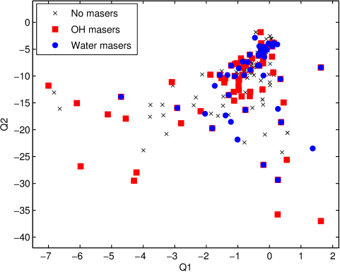
Figure 4: $Q1$–$Q2$ diagram of the objects observed in the current project. The OH and H₂O sources are specified by the filled red squares and filled blue circles, respectively. The H₂O detections in Paper I are also included. Many of them are AGB stars. The non-detections are specified by the black crosses.

where $J$ (1.25 $\mu$m), $H$ (1.65 $\mu$m), and $K_{\rm s}$ (2.17 $\mu$m) represent the three band fluxes of the Two Micron All Sky Survey (2MASS, Skrutskie et al., 2006), and [8.0] is the 8 $\mu$m band flux from the Galactic Legacy Infrared Mid-Plane Survey Extraordinaire (GLIMPSE, Benjamin et al., 2003; Churchwell et al., 2009). The $Q1$ parameter was originally used to select infrared counterparts of high-mass X-ray binaries, and it was also useful in finding red supergiant clusters (Negueruela & Schurch, 2007; Negueruela et al., 2011; Fok et al., 2012). The $Q2$ parameter was inspired by $Q1$, but in addition to the near-infrared 2MASS data, the mid-infrared [8.0] data were also included. This parameter could be used to measure the infrared excess due to circumstellar shells only, which is independent of interstellar extinction (Messineo et al., 2012). Therefore, comparing to $Q1$, $Q2$ is more sensitive to the nature of circumstellar envelopes of evolved stars. In Messineo et al. (2012), the [8.0] entries were preferably taken from the GLIMPSE database, because it has a high resolution ($\sim$1$\farcs$2). However, since the GLIMPSE project mainly covered the region within Galactic latitudes $b=\pm 1^{\circ}$ along most part of the Galactic plane, many of our objects are therefore not included because evolved stars tend to drift away from the Galactic plane. Thus, we have used the $A$ (8.28 $\mu$m) band data from the Midcourse Space Experiment (MSX, Egan et al., 2003) instead of GLIMPSE. It was shown that this change would not alter the behaviour of the $Q2$ parameter (see Figure 4 in Messineo et al., 2012). Since $Q1$ and $Q2$ serve like colours (but free from the effect of interstellar extinction) which are affected by the profile of the spectral energy distributions (SEDs), it is expected that most of the objects at the same stage of stellar evolution will share the same ranges of $Q$ values. Hence, they will cluster in the $Q1$–$Q2$ diagram, similar to the cases of 2-colour diagrams (see, e.g., IRAS 2-colour diagram, van der Veen & Habing, 1988). Figure 4 shows the $Q1$–$Q2$ diagram of the observed targets in this project, together with the H₂O sources detected in Paper I. The objects are found within $-7<Q1<2$ and $-37<Q2<0$, but most of them are distributed roughly in the cluster with $-2<Q1<1$ and $-15<Q2<0$. Some objects extend from this main cluster toward the negative $Q2$ direction, while some others are found in another region with more negative $Q1$ values. The range of $Q2$ values occupied by our maser sources is larger when compared to the range of $Q1$ values, that means the objects have a wider range of flux values in the mid- or far- infrared regions (reflected by $Q2$), than in the near-infrared region (reflected by $Q1$).

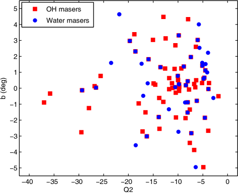
Figure 5: Galactic latitude, $b$, versus $Q2$ (see eq. (2)) of the OH and H₂O sources detected in the current observation or Paper I.

Before any further discussion, we have to consider the possible influence of artificial effects or contamination. The interstellar extinction has been a big problem for infrared research, and the situation becomes even more severe for the region toward the Galactic plane. In fact, the $Q2$ parameter was designed in a way to avoid the effect of extinction. Figure 5 shows a diagram of $Q2$ versus Galactic $b$. We can see that there are more OH maser sources in the region with $|b|<1^{\circ}$. However, the $Q2$ values of our OH and H₂O maser sources do not have a clear correlation with Galactic latitude. Hence, even if there is a positional dependence for the $Q2$ value, it is not significant. Another possible source of error comes from the resolution of the OH maser observations. Since the large beam occasionally covered more than one source with similar infrared characteristics, sometimes it is a bit difficult to confirm which source the OH maser comes from. This would not be a problem for the sources where H₂O masers were detected as well, because in those cases the origin of the OH masers could be checked by comparing the line velocities of both masers. The ambiguous cases are discussed in Section 3.2 already.

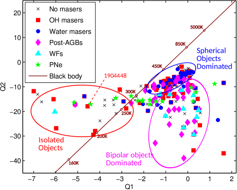
Figure 6: Same as Figure 4, but more sources such as WFs, PPNe, and PNe, are included. The objects fall into three regions. One is dominated by objects with spherical envelopes (enclosed by the blue ellipse); another one is dominated by objects associated with bipolar jets (enclosed by the purple ellipse); the third one contains the “isolated objects” (enclosed by the red ellipse). The reason for their peculiar Q values is not clear (see Section 4.1). The black body curve is shown in brown.

Figure 6 shows basically the same $Q1$–$Q2$ diagram as Figure 4, but with the addition of a number of known sources for a comparison. The PPNe were obtained from Meixner et al. (1999). The PNe were mainly selected from Ruffle et al. (2004) and the ARVAL Catalogue of Bright Planetary Nebulae. The objects form three groups in the diagram which are more or less similar to Figure 4. The group enclosed by a blue ellipse is dominated by AGB H₂O maser sources from Paper I. Many of them are still keeping a rather spherical envelope, as suggested by their spectral profiles. They have an elongated distribution pattern which roughly extends along the black body curve. The group enclosed by a purple ellipse is dominated by WFs and PPNe, which are mostly bipolar objects. These objects are expected to be more evolved than the spherical objects, based on the assumption that jets usually develop at a later stage of evolution (but recall there are exceptions such as X Her and V Hya, which are AGB stars with bipolar structure, see Section 1). Since they probably have thicker and more extended envelopes, the temperature is lower and hence the more negative $Q2$ values (about $-10$ to $-40$). The position of the new WF candidate, IRAS 19356$+$0754, is not known because we are not able to find its $Q2$ values due to insufficient photometric data. The red ellipse encloses a smaller number ($\sim$20) of objects which are isolated from the two main groups by having more negative $Q1$ values (about $-7$ to $-3$). One of the WFs, OH 12.8$-$0.9, suggested to be a late-AGB star (Boboltz & Marvel, 2005, 2007), and also the high velocity object candidate, 1904448$+$042318, are found in this group. The reason for their peculiar $Q1$ values is not clear. The PNe are mainly found in the narrow region between the above three groups (i.e. with larger $Q2$ values than the PPNe), indicating a smaller mid-infrared flux than the PPNe. This is because the hot central star will become more exposed again in the PNe phase, and therefore a larger portion of the flux will be emitted from the star in the optical or near-infrared rather than from the mid-infrared. Finally, $Q2$ could not be calculated for two representative bipolar AGB stars, X Her and V Hya, because there are no data with respect to their 8 $\mu$m flux. Their $Q1$ values are $-0.17$ and $0.08$, respectively. From Figure 6, we can see that they are unlikely to be found in the region for spherical objects, no matter what their $Q2$ values are. Instead, their $Q1$ values ($\sim$0) are in the middle of the $Q1$ range for “bipolar objects”, which agrees with their bipolar nature.

Despite the small number of exceptional cases, we find a clear separation between the spherical and bipolar objects in the $Q1$–$Q2$ diagram. Most post-AGB stars and even some late AGB stars are aspherical, in particular many of them show a certain degree of bipolarity due to jets (see Section 1). The method used here by employing the $Q1$–$Q2$ diagram could isolate the clearly aspherical objects, which are likely (but not necessarily) objects at the late AGB/post-AGB phase.

4.2 The Far-Infrared AKARI Colours

In Paper I, we have shown that the AGB and post-AGB stars occupy different regions in the AKARI [09]$-$[18] versus [18]$-$[65] two-colour diagram, suggesting that the AKARI colours are useful for studying late stage stellar evolution. Now we can extend this work by considering more known objects (Figure 7). The sample of PPNe and PNe is the same as that shown in Figure 6.

We find that the regionalization in Paper I is over simplified because the objects are assumed to move along a single trend on the diagram as they evolve. However, the object distribution in Figure 7 suggests the presence of two major groups of sources. Here most of the PPNe are found mixing with some AGB maser sources (those assumed to have spherical envelopes) and WFs, in an elongated region (purple ellipse) almost parallel to the black body curve. The AGB stars appear at the higher temperature end, while the WFs are at the lower temperature end. This temperature tendency is similar to that in the $Q1$–$Q2$ diagram. However, here we have a stronger correlation between the PPNe and the black body curve. This is presumably due to the fact that the far-infrared colours are more sensitive to the temperature of the cold dust component, which contributes most of the flux from the SEDs of PPNe (e.g., IRAS 16342$-$3814, Murakawa & Izumiura, 2012). There are some objects, which deviate from the black body curve, that occupy the region with $0<$ [09]$-$[18] $<2$ and $0<$ [18]$-$[65] $<3$ (upper part of the green ellipse). However, there is no obvious sign on which kind of specific objects would behave like that. Nonetheless, we suspect that the aspherical objects will tend to move toward this region, because the high velocity object candidate 1904448$+$042318, the known peculiar bipolar object IRAS 19312$+$1950 (Nakashima et al., 2011), and most of the selected PNe are found in this region.

Both the envelope morphology and temperature are common indicators to determine the evolutionary status of evolved stars. For instance, it is known that an AGB star usually has a spherical envelope, as opposed to the aspherical envelope of a post-AGB star, and the envelope temperature of the former is higher ($\geq$300 K). However, Figure 7 seems to suggest that the change in temperature of the objects could be independent of their morphological change. That means, it is possible to have hotter AGB-like stars which are aspherical. In fact, as we mentioned before, W 43A, X Her and V Hya are examples of AGB stars with bipolar jets. If jets can be launched before the post-AGB phase, we suspect that WFs might not necessarily represent the short “young post-AGB” episode which has been widely accepted. By studying the spectral energy distribution (SED), we found that half of the known WFs actually have characteristics of AGB stars (Yung et al. 2014, in prep.). Note that on the contrary, there are almost no spherical post-AGB stars (e.g., Lagadec et al., 2011). In short, the morphological change might not have a direct relationship to the evolutionary status: it could be safe to assume the cold post-AGB stars are aspherical, but it is not entirely correct to label all aspherical evolved stars as post-AGB stars, even though in most cases this is still true. Similar to the $Q1$–$Q2$ diagram, the AKARI two-colour diagram could serve the purpose of identifying aspherical objects without assumptions on their evolutionary status, but the AKARI colours are more sensitive to the temperatures of the colder envelopes that mainly shine at far-infrared wavelengths.

5 Summary and Conclusion

We have conducted an OH and H₂O maser survey with targets selected by the far-infrared AKARI colours. We found a new WF candidate, IRAS 19356$+$0754, and a few possible high velocity OH objects. New H₂O maser components were detected for the known WF, IRAS 18286$-$0959, which might be a hint on jet acceleration. We then studied the maser sources, and other known objects such as PPNe and PNe, using the $Q1$ and $Q2$ parameters as well as the AKARI colours. While the $Q1$–$Q2$ diagram seems to be effective in separating the spherical and bipolar objects in general, the AKARI colours show further that the morphological change in cold sources is not necessarily related to their evolutionary status, i.e., even though many of the aspherical objects are found to be post-AGB stars, some AGB stars may also develop jets before reaching the post-AGB phase. We suggest that the efficiency of identifying oxygen-rich objects during the late stages of stellar evolution (i.e. late AGB/post-AGB stars) could be improved by considering together the maser properties, the $Q$-parameters and the AKARI colours.

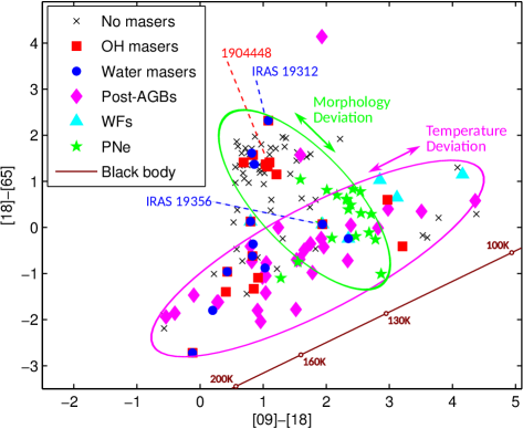
Figure 7: AKARI two-color diagram of the targets observed in the current project, the H₂O sources in Paper I, and some other known sources (same sample as in Figure 6). The objects fall into two elongated regions. The region enclosed by the purple ellipse shows clear correlation with the black body temperature (shown in brown), while the one enclosed by the green ellipse seems to be related to the morphologies (e.g. spherical or bipolar).

Table 1: Parameters of the objects observed.

Object	Other Name	R.A.	Decl.	AC12	AC23	$Q1$	$Q2$	OH	H2O
0038592$+$592746	INS2001 J003859.4$+$592749	00 38 59.28	$+$59 27 46.9	0.75	1.35	$-$0.49	$-$9.84	$\cdots$	N
0122182$+$634055	$\cdots$	01 22 18.28	$+$63 40 55.3	0.56	1.31	$-$0.55	$-$9.39	$\cdots$	N
0128404$+$632737	$\cdots$	01 28 40.47	$+$63 27 37.9	0.60	1.76	$-$0.62	$-$9.42	$\cdots$	N
0253373$+$691539	IRAS 02490$+$6903	02 53 37.39	$+$69 15 39.2	1.54	1.63	$-$4.10	$\cdots$	$\cdots$	N
0358076$+$624425	$\cdots$	03 58 07.65	$+$62 44 25.8	0.70	1.06	$-$1.13	$\cdots$	$\cdots$	N
0413220$+$501428	IRAS 04096$+$5006	04 13 22.07	$+$50 14 28.2	0.66	1.61	$-$1.34	$-$9.70	$\cdots$	N
0433014$+$343840	IRAS 04297$+$3432	04 33 01.45	$+$34 38 40.6	1.12	0.37	$-$0.78	$\cdots$	$\cdots$	N
0536468$+$314600	IRAS 05335$+$3144	05 36 46.88	$+$31 46 00.2	0.94	1.36	0.02	$-$7.73	$\cdots$	N
0540502$+$340241	$\cdots$	05 40 50.22	$+$34 02 41.3	0.82	1.71	0.16	$\cdots$	$\cdots$	N
0547450$+$003842	2MASS J05474500$+$0038418	05 47 45.00	$+$00 38 42.1	1.02	1.18	$-$0.50	$\cdots$	$\cdots$	N
0608452$+$130841	$\cdots$	06 08 45.28	$+$13 08 41.3	1.53	1.45	$-$3.06	$-$11.76	$\cdots$	N
IRAS 16030$-$0634	$\cdots$	16 05 46.33	$-$06 42 27.9	$-$0.46	$\cdots$	$-$0.16	$\cdots$	N	N
IRAS 16131$-$0216	$\cdots$	16 15 47.66	$-$02 23 31.9	$-$0.64	$\cdots$	0.28	$\cdots$	N	N
IRAS 17055$-$0216	$\cdots$	17 08 10.20	$-$02 20 21.0	$-$0.22	$\cdots$	$-$0.63	$\cdots$	N	Y
IRAS 17132$-$0744	$\cdots$	17 15 56.40	$-$07 47 33.0	$\cdots$	$\cdots$	$\cdots$	$\cdots$	N	Y
IRAS 17171$-$0843	$\cdots$	17 19 53.45	$-$08 46 59.7	$-$0.11	$\cdots$	$-$0.70	$\cdots$	$\cdots$	Y
IRAS 17193$-$0601	$\cdots$	17 22 02.30	$-$06 04 13.0	$-$0.46	$\cdots$	$-$0.05	$\cdots$	N	N
IRAS 17343$+$1052	$\cdots$	17 36 44.45	$+$10 51 07.0	$-$0.72	$\cdots$	0.01	$\cdots$	$\cdots$	Y
1741385$-$241435	IRAS 17385$-$2413	17 41 38.52	$-$24 14 35.8	1.22	$-$0.90	0.40	$-$24.21	$\cdots$	N
1750356$-$203743	IRAS 17476$-$2036	17 50 35.60	$-$20 37 43.5	0.58	$-$0.47	$-$0.72	$-$7.88	N	N
1752536$-$184100	$\cdots$	17 52 53.68	$-$18 41 00.8	0.74	$-$1.44	$-$6.64	$-$16.10	$\cdots$	N
1807272$-$194639	IRAS 18044$-$1947	18 07 27.26	$-$19 46 39.3	0.92	$-$1.09	$-$1.43	$-$11.22	Y	N
IRAS 18056$-$1514	$\cdots$	18 08 28.40	$-$15 13 30.0	0.43	$-$0.96	0.37	$-$18.59	Y	Y
IRAS 18099$-$1449	$\cdots$	18 12 47.37	$-$14 48 50.0	$-$0.68	$\cdots$	$-$0.08	$-$5.11	N	Y
IRAS 18100$-$1250	$\cdots$	18 12 50.49	$-$12 49 44.8	$-$0.39	$\cdots$	$-$0.17	$-$5.68	N	Y
IRAS 18117$-$1625	$\cdots$	18 14 38.70	$-$16 24 39.0	0.04	$\cdots$	$-$1.21	$-$8.05	Y	Y
IRAS 18118$-$1615	$\cdots$	18 14 41.35	$-$16 14 03.0	0.47	$\cdots$	$-$1.09	$-$9.99	Y	N
IRAS 18127$-$1516	$\cdots$	18 15 39.90	$-$15 15 13.0	$\cdots$	$\cdots$	$-$1.10	$-$10.05	Y	Y
1824037$+$063625	IRAS 18216$+$0634	18 24 03.72	$+$06 36 25.8	0.85	$-$1.33	$-$1.19	$\cdots$	Y	N
1824288$-$155108	IRAS 18216$-$1552	18 24 28.88	$-$15 51 09.0	0.22	$-$1.01	$-$3.39	$-$15.35	$\cdots$	N
IRAS 18251$-$1048	$\cdots$	18 27 56.30	$-$10 46 58.0	0.80	$\cdots$	$-$1.57	$-$9.80	Y	$\cdots$
IRAS 18286$-$0959	$\cdots$	18 31 22.93	$-$09 57 21.7	0.80	0.13	0.27	$-$29.35	Y	Y
OH 16.3$-$3.0	TVH89 313	18 31 31.51	$-$16 08 46.5	0.83	$-$0.62	$-$0.76	$-$16.30	Y	Y
IRAS 18362$-$0521	$\cdots$	18 38 57.47	$-$05 18 28.0	$\cdots$	$\cdots$	$-$0.10	$-$5.51	$\cdots$	N
1838595$-$052024	IRAS 18363$-$0523	18 38 59.57	$-$05 20 24.0	0.41	$-$1.40	$-$0.27	$-$5.15	Y	N
1848010$+$000448	IRAS 18454$+$0001	18 48 01.09	$+$00 04 48.6	4.08	1.30	$-$0.19	$-$12.53	$\cdots$	N
IRAS 18455$+$0448	$\cdots$	18 48 02.30	$+$04 51 30.5	1.03	$-$0.88	$-$1.81	$-$19.73	$\cdots$	Y
1854158$+$011501	$\cdots$	18 54 15.85	$+$01 15 01.8	0.84	1.57	$-$7.00	$-$11.79	Y	N
1854250$+$004958	MSX6C G034.0126$-$00.2832	18 54 25.10	$+$00 49 58.2	0.69	1.41	$-$1.40	$-$10.46	Y	N
IRAS 18587$+$0521A	$\cdots$	19 01 08.43	$+$05 25 48.0	$-$0.05	$\cdots$	0.08	$-$3.75	$\cdots$	N
IRAS 18587$+$0521	$\cdots$	19 01 10.70	$+$05 25 46.0	$\cdots$	$\cdots$	0.58	$\cdots$	Y	$\cdots$
IRAS 18587$+$0521B	$\cdots$	19 01 12.40	$+$05 25 43.4	1.95	$\cdots$	0.27	$-$16.12	$\cdots$	Y
IRAS 18596$+$0605	$\cdots$	19 02 04.69	$+$06 10 09.5	0.04	$\cdots$	$-$0.28	$-$5.78	$\cdots$	N
1904448$+$042318	SSTGLMC G038.3546$-$00.9519	19 04 44.90	$+$04 23 18.2	1.10	1.41	$-$4.55	$-$17.93	Y	N
IRAS 19027$+$0517	$\cdots$	19 05 14.28	$+$05 21 52.2	0.35	$\cdots$	$-$0.88	$-$13.79	Y	N
IRAS 19074$+$0534	$\cdots$	19 09 54.81	$+$05 39 06.9	1.04	1.37	$-$2.18	$-$16.56	Y	N
IRAS 19085$+$1038	$\cdots$	19 10 57.20	$+$10 43 38.0	$\cdots$	$\cdots$	0.19	$\cdots$	N	N
1911358$+$133111	IRAS 19092$+$1326	19 11 35.85	$+$13 31 11.1	1.74	0.44	$-$1.85	$-$17.00	N	N
1912477$+$033435	$\cdots$	19 12 47.75	$+$03 34 35.8	3.78	0.21	$-$0.23	$-$12.80	N	N
1914408$+$114449	IRAS 19123$+$1139	19 14 40.83	$+$11 44 49.4	1.21	1.15	$-$0.90	$-$6.73	Y	N
IRAS 19134$+$2131	$\cdots$	19 15 35.19	$+$21 36 33.6	2.35	$-$0.24	$-$1.01	$-$21.84	N	Y
1918205$+$014659	V⁢ V605 Aql	19 18 20.57	$+$01 46 59.0	1.83	0.60	$-$0.43	$\cdots$	N	N
1919572$+$104808	IRAS 19175$+$1042	19 19 57.24	$+$10 48 08.8	0.84	$-$0.36	$-$1.73	$-$11.84	$\cdots$	Y
1922250$+$131851	IRAS 19201$+$1313	19 22 25.08	$+$13 18 51.6	0.87	1.97	$-$2.33	$-$14.00	$\cdots$	N
1922557$+$202854	IRAS 19207$+$2023	19 22 55.78	$+$20 28 54.3	3.21	$-$0.41	0.08	$-$6.40	Y	N
1923002$+$151051	IRAS 19207$+$1504	19 23 00.28	$+$15 10 51.3	0.67	$-$0.73	$-$1.47	$-$15.53	$\cdots$	N
1930003$+$175601	MSX6C G053.2176$-$00.0808	19 30 00.30	$+$17 56 01.7	1.07	1.32	$-$1.09	$-$7.78	Y	N
IRAS 19312$+$1950	$\cdots$	19 33 24.30	$+$19 56 55.0	1.08	2.32	1.63	$-$8.42	Y	Y
IRAS 19356$+$0754	$\cdots$	19 38 01.19	$+$08 01 33.0	1.94	0.07	$-$1.13	$\cdots$	Y	Y
1938574$+$103016	IRAS19365+1023	19 38 57.42	$+$10 30 16.0	0.53	0.11	$-$0.23	$\cdots$	N	N
IRAS 19464$+$3514	$\cdots$	19 48 15.96	$+$35 22 06.1	0.20	$-$1.80	$-$1.17	$\cdots$	$\cdots$	Y
1951461$+$272458	2MASS J19514615$+$2724587	19 51 46.20	$+$27 24 58.5	0.82	1.61	$-$1.33	$-$9.83	N	Y
IRAS 20010$+$2508	$\cdots$	20 03 08.30	$+$25 17 27.0	$-$0.75	$\cdots$	$-$0.24	$-$1.90	N	N
2003357$+$284847	IRAS 20015$+$2840	20 03 35.71	$+$28 48 47.2	1.75	1.59	$-$0.65	$\cdots$	N	N
2003599$+$351617	$\cdots$	20 03 59.97	$+$35 16 17.9	0.58	1.86	$-$0.50	$-$8.39	N	N
IRAS 20021$+$2156	$\cdots$	20 04 17.30	$+$22 04 59.0	$-$0.27	$\cdots$	$-$0.16	$-$6.44	N	Y
2008383$+$410040	IRAS 20068$+$4051	20 08 38.39	$+$41 00 40.4	2.22	1.92	0.14	$-$9.79	N	N
2009217$+$271859	IRAS 20072$+$2710	20 09 21.72	$+$27 18 59.2	0.94	1.26	$-$0.56	$-$7.68	$\cdots$	N
2013142$+$370536	IRAS 20113$+$3656	20 13 14.22	$+$37 05 36.9	1.01	0.94	$-$0.77	$-$8.80	$\cdots$	N
2015573$+$470534	IRAS 20144$+$4656	20 15 57.33	$+$47 05 34.5	2.97	0.60	$-$1.11	$\cdots$	Y	N
2020151$+$364334	$\cdots$	20 20 15.14	$+$36 43 34.5	1.10	1.58	$-$0.98	$-$9.59	$\cdots$	N
IRAS 20215$+$6243	$\cdots$	20 22 20.05	$+$62 53 02.2	$-$0.56	$\cdots$	$-$0.08	$\cdots$	N	N
2029222$+$403543	IRAS 20275$+$4025	20 29 22.22	$+$40 35 43.5	1.20	1.71	$-$2.40	$-$15.46	$\cdots$	N
IRAS 20305$+$6246	$\cdots$	20 31 26.54	$+$62 56 49.8	$-$0.89	$\cdots$	$-$0.22	$\cdots$	N	N
2033464$+$450840	MSX6C G083.3609$+$02.9902	20 33 46.48	$+$45 08 40.4	1.31	$-$0.24	$-$1.63	$-$17.41	$\cdots$	N
2040444$+$465322	IRAS 20390$+$4642	20 40 44.45	$+$46 53 22.4	0.56	0.97	$-$0.97	$-$10.08	N	N
2048044$+$390459	IRAS 20461$+$3853	20 48 04.41	$+$39 04 59.7	1.83	$-$0.46	0.02	$-$11.73	N	N
2048166$+$342724	IRAS 20462$+$3416	20 48 16.64	$+$34 27 24.4	4.38	0.29	$-$0.12	$\cdots$	N	N
2050135$+$594551	IRAS 20490$+$5934	20 50 13.58	$+$59 45 51.2	1.61	0.63	$-$0.58	$\cdots$	N	N
2053379$+$445807	MSX6C G085.3935$+$00.1268	20 53 37.98	$+$44 58 07.4	0.91	$-$0.65	$-$5.98	$-$26.82	$\cdots$	N
2057130$+$482200	IRAS 20555$+$4810	20 57 13.08	$+$48 22 00.3	0.72	1.72	$-$0.54	$-$15.92	$\cdots$	N
2100253$+$523017	V⁢ V2495 Cyg	21 00 25.34	$+$52 30 17.6	1.34	1.75	$\cdots$	$\cdots$	$\cdots$	N
2101550$+$495135	IRAS 21002$+$4939	21 01 55.02	$+$49 51 35.5	0.77	0.97	$-$0.58	$-$7.37	$\cdots$	N
2117391$+$685509	IRAS 21169$+$6842	21 17 39.18	$+$68 55 09.5	1.13	0.60	$-$0.62	$\cdots$	$\cdots$	N
2122090$+$492624	$\cdots$	21 22 09.06	$+$49 26 24.5	0.59	0.38	$-$0.81	$-$9.28	$\cdots$	N
IRAS 21509$+$6234	$\cdots$	21 52 19.37	$+$62 48 39.5	$-$0.41	$\cdots$	0.07	$\cdots$	N	N
IRAS 21522$+$6018	$\cdots$	21 53 46.10	$+$60 32 14.2	$-$0.55	$\cdots$	$-$0.14	$\cdots$	N	Y
2155455$+$575106	IRAS 21541$+$5736	21 55 45.55	$+$57 51 06.6	1.31	1.96	$-$0.79	$-$8.98	$\cdots$	N
IRAS 21563$+$5630	$\cdots$	21 58 01.30	$+$56 44 49.6	$-$0.58	$-$1.90	$-$0.32	$-$4.45	N	N
2158358$+$585722	2MASS J21583590$+$5857227	21 58 35.81	$+$58 57 22.8	0.79	1.59	$-$1.51	$-$9.08	$\cdots$	N
2204124$+$530401	IRAS 22023$+$5249	22 04 12.45	$+$53 04 02.0	3.53	$-$0.17	$-$0.22	$-$14.38	$\cdots$	N
IRAS 22097$+$5647	$\cdots$	22 11 31.88	$+$57 02 17.4	$-$0.12	$-$2.72	$-$0.15	$-$4.69	Y	Y
2219055$+$613616	IRAS 22174$+$6121	22 19 05.52	$+$61 36 16.1	0.63	1.34	$-$0.70	$-$10.34	$\cdots$	N
2219520$+$633532	IRAS 22182$+$6320	22 19 52.05	$+$63 35 32.4	0.68	1.18	$-$0.74	$\cdots$	$\cdots$	N
2233550$+$653918	$\cdots$	22 33 55.02	$+$65 39 18.5	1.12	1.73	$-$6.28	$\cdots$	$\cdots$	N
IRAS 22394$+$6930	$\cdots$	22 40 59.80	$+$69 46 14.7	$-$0.63	$\cdots$	$-$0.08	$\cdots$	Y	Y
IRAS 22394$+$5623	$\cdots$	22 41 27.10	$+$56 39 08.0	$-$0.71	$\cdots$	0.02	$-$2.58	$\cdots$	N
2251389$+$515042	IRAS 22495$+$5134	22 51 38.97	$+$51 50 42.7	3.60	$-$0.22	$-$0.24	$\cdots$	$\cdots$	N
2259442$+$585956	IRAS 22576$+$5843	22 59 44.21	$+$58 59 56.2	1.36	1.94	$-$1.62	$\cdots$	$\cdots$	N
2303421$+$614741	$\cdots$	23 03 42.15	$+$61 47 41.4	0.86	1.37	$-$1.39	$-$17.34	$\cdots$	Y
2312291$+$612534	IRAS 23103$+$6109	23 12 29.16	$+$61 25 34.1	1.69	1.53	0.57	$-$20.58	$\cdots$	N
2317522$+$580511	IRAS 23156$+$5748	23 17 52.22	$+$58 05 11.2	1.43	1.16	$-$1.05	$-$9.27	$\cdots$	N
2335128$+$610005	IRAS 23328$+$6043	23 35 12.84	$+$61 00 05.4	0.97	1.80	$-$2.13	$-$9.73	$\cdots$	N
2341559$+$641512	IRAS 23395$+$6358	23 41 55.98	$+$64 15 12.5	0.76	1.63	$-$0.34	$-$7.54	$\cdots$	N
2346058$+$632312	IRAS 23436$+$6306	23 46 05.81	$+$63 23 12.8	0.95	1.19	$-$0.27	$-$10.85	$\cdots$	N
IRAS 23489$+$6235	$\cdots$	23 51 27.28	$+$62 51 47.1	$-$1.44	$\cdots$	$-$0.43	$-$1.84	$\cdots$	N
IRAS 23554$+$5612	$\cdots$	23 58 01.32	$+$56 29 13.4	$-$0.57	$-$2.19	$-$0.41	$\cdots$	$\cdots$	N
IRAS 23561$+$6037	$\cdots$	23 58 38.70	$+$60 53 48.0	$-$0.78	$\cdots$	0.06	$-$3.13	$\cdots$	N

Table 2: Parameters of the OH maser detections.

Object	Rest Freq.	$V_{\rm b,p}$	$F_{\rm b,p}$	$V_{\rm r,p}$	$F_{\rm r,p}$	$V_{\rm b,e}$	$V_{\rm r,e}$	$I$	rms	Ref.	Absorptions
	(MHz)	( km s-1)	(Jy)	( km s-1)	(Jy)	( km s-1)	( km s-1)	(Jy  km s-1)	(Jy)		( km s-1)
1807272$-$194639	1612	$-$48.4	0.62	$\cdots$	$\cdots$	$-$77.4	30.4	2.71	0.03	new	$\cdots$
	1665	$\cdots$	$\cdots$	$\cdots$	$\cdots$	$\cdots$	$\cdots$	$\cdots$	0.03	$\cdots$	32.2
	1667	$-$76.3	0.88	$-$45.5	0.28	$-$77.9	$-$43.3	2.69	0.03	1	26.9
IRAS 18056$-$1514	1612	46.9	2.44	71.9	1.60	45.2	73.0	6.84	0.02	2	$\cdots$
	1665	$\cdots$	$\cdots$	$\cdots$	$\cdots$	$\cdots$	$\cdots$	$\cdots$	0.02	$\cdots$	$\cdots$
	1667	$\cdots$	$\cdots$	$\cdots$	$\cdots$	$\cdots$	$\cdots$	$\cdots$	0.01	$\cdots$	$\cdots$
IRAS 18117$-$1625	1612	65.1	0.31	101.4	0.19	63.9	102.5	0.55	0.03	new	$\cdots$
	1665	$\cdots$	$\cdots$	$\cdots$	$\cdots$	$\cdots$	$\cdots$	$\cdots$	0.02	$\cdots$	$\cdots$
	1667	$\cdots$	$\cdots$	$\cdots$	$\cdots$	$\cdots$	$\cdots$	$\cdots$	0.03	$\cdots$	$\cdots$
IRAS 18118$-$1615	1612	162.7	0.24	$\cdots$	$\cdots$	161.5	163.8	0.24	0.02	new	$\cdots$
	1665	$\cdots$	$\cdots$	$\cdots$	$\cdots$	$\cdots$	$\cdots$	$\cdots$	0.02	$\cdots$	$\cdots$
	1667	170.1	0.09	$\cdots$	$\cdots$	160.0	178.0	0.42	0.02	new	$\cdots$
IRAS 18127$-$1516	1612	$-$18.9	0.22	18.0	0.06	$-$20.1	20.0	0.71	0.01	new	$\cdots$
	1665	$\cdots$	$\cdots$	$\cdots$	$\cdots$	$\cdots$	$\cdots$	$\cdots$	0.01	$\cdots$	$\cdots$
	1667	$\cdots$	$\cdots$	$\cdots$	$\cdots$	$\cdots$	$\cdots$	$\cdots$	0.01	$\cdots$	$\cdots$
1824037$+$063625	1612	$\cdots$	$\cdots$	$\cdots$	$\cdots$	$\cdots$	$\cdots$	$\cdots$	0.01	$\cdots$	$\cdots$
	1665	$\cdots$	$\cdots$	$\cdots$	$\cdots$	$\cdots$	$\cdots$	$\cdots$	0.01	$\cdots$	$\cdots$
	1667	$-$29.1	0.11	$-$10.4	0.12	$-$30.1	$-$9.9	0.28	0.02	new	$\cdots$
IRAS 18251$-$1048	1612	71.3	1.49	111.0	2.17	67.9	112.2	10.55	0.03	3	81.5
	1665	$\cdots$	$\cdots$	$\cdots$	$\cdots$	$\cdots$	$\cdots$	$\cdots$	0.04	$\cdots$	$\cdots$
	1667	23.0	0.14	113.0	0.17	9.3	126.2	3.87	0.03	3	7.1
IRAS 18286$-$0959	1612	$-$0.2	0.15	12.3	0.10	$-$2.5	14.0	0.50	0.02	4	$\cdots$
	1665	$\cdots$	$\cdots$	$\cdots$	$\cdots$	$\cdots$	$\cdots$	$\cdots$	0.02	$\cdots$	4.2
	1667	$\cdots$	$\cdots$	$\cdots$	$\cdots$	$\cdots$	$\cdots$	$\cdots$	0.02	$\cdots$	6.0
OH 16.3$-$3.0	1612	20.8	8.09	35.0	6.98	11.2	45.2	41.37	0.02	4	$\cdots$
	1665	21.2	0.06	$\cdots$	$\cdots$	20.1	30.0	0.31	0.01	new	$\cdots$
	1667	45.5	0.22	$\cdots$	$\cdots$	24.7	46.6	1.05	0.01	new	$\cdots$
1838595$-$052024	1612	41.2	0.13	$\cdots$	$\cdots$	40.1	44.1	0.23	0.02	new	67.3, 102.5
	1665	$\cdots$	$\cdots$	$\cdots$	$\cdots$	$\cdots$	$\cdots$	$\cdots$	0.02	$\cdots$	$\cdots$
	1667	21.4	0.07	$\cdots$	$\cdots$	17.6	59.8	0.75	0.02	new	$\cdots$
1854158$+$011501	1612	19.1	0.41	45.8	0.86	18.0	46.9	2.85	0.02	new	$\cdots$
	1665	36.6	0.07	$\cdots$	$\cdots$	33.9	40.5	0.33	0.02	new	$\cdots$
	1667	37.3	0.13	$\cdots$	$\cdots$	32.9	41.1	0.69	0.02	new	12.6, 29.1, 55.4
1854250$+$004958	1612	12.3	0.14	$\cdots$	$\cdots$	8.9	13.4	0.33	0.02	new	$\cdots$
	1665	$\cdots$	$\cdots$	$\cdots$	$\cdots$	$\cdots$	$\cdots$	$\cdots$	0.02	$\cdots$	21.8
	1667	$\cdots$	$\cdots$	$\cdots$	$\cdots$	$\cdots$	$\cdots$	$\cdots$	0.02	$\cdots$	13.1
IRAS 18587$+$0521	1612	$-$15.5	0.08	33.9	0.05	$-$17.2	35.6	$-$0.58	0.01	new	$\cdots$
	1665	$\cdots$	$\cdots$	$\cdots$	$\cdots$	$\cdots$	$\cdots$	$\cdots$	0.01	$\cdots$	$-$14.5, 14.6
	1667	24.1	0.04	$\cdots$	$\cdots$	20.8	25.8	0.16	0.01	new	$\cdots$
1904448$+$042318	1612	15.7	0.13	76.4	0.32	12.3	88.9	2.27	0.02	new	20.8
	1665	63.5	0.20	$\cdots$	$\cdots$	16.8	91.0	1.51	0.02	new	20.1
	1667	17.0	0.41	$\cdots$	$\cdots$	12.6	91.1	2.83	0.02	new	$\cdots$
IRAS 19027$+$0517	1612	13.4	0.15	$\cdots$	$\cdots$	11.2	18.0	0.44	0.02	new	82.1
	1665	32.8	0.05	77.3	0.10	28.9	85.0	1.32	0.02	new	$\cdots$
	1667	78.4	0.14	$\cdots$	$\cdots$	12.6	86.7	1.86	0.02	new	$\cdots$
IRAS 19074$+$0534	1612	12.3	0.06	$\cdots$	$\cdots$	11.1	13.4	0.07	0.01	new	$\cdots$
	1665	$\cdots$	$\cdots$	$\cdots$	$\cdots$	$\cdots$	$\cdots$	$\cdots$	0.01	$\cdots$	78.3
	1667	$\cdots$	$\cdots$	$\cdots$	$\cdots$	$\cdots$	$\cdots$	$\cdots$	0.01	$\cdots$	76.3
1914408$+$114449	1612	$\cdots$	$\cdots$	$\cdots$	$\cdots$	$\cdots$	$\cdots$	$\cdots$	0.02	$\cdots$	21.4, 59.4
	1665	59.7	0.10	$\cdots$	$\cdots$	58.0	64.1	0.29	0.02	new	$\cdots$
	1667	$\cdots$	$\cdots$	$\cdots$	$\cdots$	$\cdots$	$\cdots$	$\cdots$	0.02	$\cdots$	$\cdots$
1922557$+$202854	1612	$-$5.3	3.68	12.9	3.15	$-$8.7	14.6	14.88	0.01	new	$\cdots$
	1665	$-$6.8	0.07	11.9	0.12	$-$7.8	13.5	0.62	0.01	new	$\cdots$
	1667	$\cdots$	$\cdots$	$\cdots$	$\cdots$	$\cdots$	$\cdots$	$\cdots$	0.01	$\cdots$	7.1
1930003$+$175601	1612	23.6	0.13	$\cdots$	$\cdots$	20.8	25.3	0.33	0.02	new	$\cdots$
	1665	$\cdots$	$\cdots$	$\cdots$	$\cdots$	$\cdots$	$\cdots$	$\cdots$	0.02	$\cdots$	25.1
	1667	$\cdots$	$\cdots$	$\cdots$	$\cdots$	$\cdots$	$\cdots$	$\cdots$	0.02	$\cdots$	25.7
IRAS 19312$+$1950	1612	28.7	0.81	$\cdots$	$\cdots$	10.0	36.7	3.66	0.02	5	$\cdots$
	1665	32.8	0.10	$\cdots$	$\cdots$	29.5	42.7	0.71	0.02	5	$\cdots$
	1667	30.2	0.13	$\cdots$	$\cdots$	28.0	39.0	0.81	0.02	5	$\cdots$
IRAS 19356$+$0754	1612	$-$119.9	3.83	$\cdots$	$\cdots$	$-$138.1	$-$71.1	48.87	0.02	new	$\cdots$
	1665	$-$94.7	0.87	$\cdots$	$\cdots$	$-$134.8	$-$74.3	11.67	0.02	new	$\cdots$
	1667	$-$133.3	0.35	$\cdots$	$\cdots$	$-$138.8	$-$87.2	8.58	0.02	new	$\cdots$
2015573$+$470534	1612	$-$9.3	5.15	$-$0.8	2.61	$-$13.2	7.2	24.05	0.01	new	$\cdots$
	1665	$-$6.8	0.22	$-$2.9	0.13	$-$8.4	$-$1.3	0.70	0.01	new	$\cdots$
	1667	$-$10.4	0.98	$\cdots$	$\cdots$	$-$12.6	10.4	4.46	0.01	new	$\cdots$
IRAS 22097$+$5647	1612	$\cdots$	$\cdots$	$\cdots$	$\cdots$	$\cdots$	$\cdots$	$\cdots$	0.01	$\cdots$	$\cdots$
	1665	63.9	0.18	$-$33.7	0.10	$-$69.4	$-$28.6	0.97	0.01	new	$\cdots$
	1667	$-$65.3	0.64	$-$43.9	0.14	$-$66.4	$-$34.0	1.87	0.01	new	$\cdots$
IRAS 22394$+$6930	1612	$-$49.6	0.13	$\cdots$	$\cdots$	$-$50.7	$-$47.3	0.19	0.01	new	$\cdots$
	1665	$\cdots$	$\cdots$	$\cdots$	$\cdots$	$\cdots$	$\cdots$	$\cdots$	0.01	$\cdots$	$\cdots$
	1667	$\cdots$	$\cdots$	$\cdots$	$\cdots$	$\cdots$	$\cdots$	$\cdots$	0.01	$\cdots$	$\cdots$

References. (1) David et al. (1993), (2) te Lintel Hekkert (1991), (3) Engels & Jimenez-Esteban (2007), (4) Sevenster et al. (2001), (5) Nakashima et al. (2011)

Table 3: Parameters of the H₂O maser detections.

Object	$V_{\rm b,p}$	$F_{\rm b,p}$	$V_{\rm r,p}$	$F_{\rm r,p}$	$V_{\rm b,e}$	$V_{\rm r,e}$	$I$	rms	Ref.
	( km s-1)	(Jy)	( km s-1)	(Jy)	( km s-1)	( km s-1)	(Jy  km s-1)	(Jy)
IRAS 17055$-$0216	$-$46.7	0.49	$\cdots$	$\cdots$	$-$47.5	$-$45.9	0.47	0.04	new
IRAS 17132$-$0744	3.9	2.16	$\cdots$	$\cdots$	$-$2.3	12.1	5.93	0.07	1
IRAS 17171$-$0843	$-$26.7	0.20	$-$9.1	0.48	$-$27.2	$-$7.6	1.12	0.06	1
IRAS 17343$+$1052	$-$57.0	0.26	$\cdots$	$\cdots$	$-$57.4	$-$56.6	0.16	0.05	2
IRAS 18056$-$1514	52.9	24.26	$\cdots$	$\cdots$	50.8	63.8	62.49	0.05	1
IRAS 18099$-$1449	$-$1.6	0.19	8.6	0.16	$-$2.9	11.1	0.76	0.04	new
IRAS 18100$-$1250	79.8	1.25	$\cdots$	$\cdots$	78.2	80.7	1.34	0.06	new
IRAS 18117$-$1625	68.5	0.15	$\cdots$	$\cdots$	67.7	69.1	0.16	0.04	new
IRAS 18127$-$1516	$-$15.4	4.53	13.2	0.20	$-$17.7	14.0	9.57	0.06	new
IRAS 18286$-$0959	62.3	22.41	$\cdots$	$\cdots$	$-$118.9	231.0	741.01	0.05	1
OH 16.3$-$3.0	19.8	0.60	39.7	0.91	14.6	42.0	4.40	0.06	1
IRAS 18455$+$0448	21.4	0.69	46.7	2.20	14.0	50.2	4.26	0.07	1
IRAS 18587$+$0521B	$-$26.3	0.53	18.9	0.40	$-$27.4	19.5	0.94	0.04	new
IRAS 19134$+$2131	$-$41.1	0.42	$-$12.3	2.27	$-$42.0	$-$8.4	5.63	0.06	3
1919572$+$104808	31.9	0.95	53.3	0.22	31.1	53.9	1.19	0.07	4
IRAS 19312$+$1950	17.3	2.44	$\cdots$	$\cdots$	14.4	23.9	5.57	0.06	5
IRAS 19356$+$0754	$-$35.3	0.19	$\cdots$	$\cdots$	$-$144.7	$-$26.2	0.45	0.01	new
IRAS 19464$+$3514	33.3	0.69	$\cdots$	$\cdots$	32.3	33.9	0.62	0.09	1
1951461$+$272458	32.3	0.48	$\cdots$	$\cdots$	29.4	32.7	0.54	0.07	new
IRAS 20021$+$2156	20.2	0.22	$\cdots$	$\cdots$	19.1	21.0	0.27	0.04	new
IRAS 21522$+$6018	20.4	0.32	$\cdots$	$\cdots$	19.8	21.0	0.23	0.04	new
IRAS 22097$+$5647	$-$49.2	54.99	$\cdots$	$\cdots$	$-$60.9	$-$39.3	81.84	0.08	1
IRAS 22394$+$6930	$-$44.6	1.05	$\cdots$	$\cdots$	$-$45.5	$-$43.2	1.18	0.05	new
2303421$+$614741	$-$8.4	0.51	2.3	0.19	$-$9.1	2.9	0.73	0.04	new

References. (1) Paper I, (2) Benson & Little-Marenin (1996), (3) Imai et al. (2007), (4) Engels & Lewis (1996), (5) Nakashima et al. (2011).

Table 4: Parameters of the OH maser non-detections. The channel spacing of the spectrometer was between 0.5 km s^-1 and 0.6 km s^-1.

Object	rms (Jy)
	1612 MHz	1665 MHz	1667 MHz
IRAS 16030$-$0634	0.03	0.05	0.03
IRAS 16131$-$0216	0.02	0.02	0.02
IRAS 17055$-$0216	0.02	0.02	0.02
IRAS 17132$-$0744	0.25	0.02	0.02
IRAS 17193$-$0601	0.03	0.02	0.02
1750356$-$203743	0.02	0.02	0.02
IRAS 18099$-$1449	0.02	0.02	0.02
IRAS 18100$-$1250	0.01	0.01	0.01
IRAS 19085$+$1038	0.02	0.02	0.02
1911358$+$133111	0.02	0.01	0.01
1912477$+$033435	0.02	0.02	0.02
IRAS 19134$+$2131	0.01	0.01	0.01
1918205$+$014659	0.02	0.02	0.02
1938574$+$103016	0.02	0.02	0.02
1951461$+$272458	0.02	0.02	0.02
IRAS 20010$+$2508	0.01	0.01	0.01
2003357$+$284847	0.02	0.02	0.02
2003599$+$351617	0.02	0.02	0.02
IRAS 20021$+$2156	0.01	0.01	0.01
2008383$+$410040	0.01	0.01	0.01
IRAS 20215$+$6243	0.01	0.01	0.01
IRAS 20305$+$6246	0.02	0.02	0.02
2040444$+$465322	0.02	0.02	0.02
2048044$+$390459	0.02	0.02	0.02
2048166$+$342724	0.02	0.02	0.01
2050135$+$594551	0.02	0.02	0.02
IRAS 21509$+$6234	0.01	0.01	0.01
IRAS 21522$+$6018	0.02	0.02	0.02
IRAS 21563$+$5630	0.01	0.01	0.01

Table 5: Parameters of the H₂O maser non-detections. The channel spacing of the spectrometer was about 0.8 km s^-1.

Object	rms (Jy)
0038592$+$592746	0.06
0122182$+$634055	0.06
0128404$+$632737	0.06
0253373$+$691539	0.06
0358076$+$624425	0.06
0413220$+$501428	0.07
0433014$+$343840	0.09
0536468$+$314600	0.08
0540502$+$340241	0.08
0547450$+$003842	0.09
0608452$+$130841	0.08
IRAS 16030$-$0634	0.07
IRAS 16131$-$0216	0.06
IRAS 17193$-$0601	0.06
1741385$-$241435	0.10
1750356$-$203743	0.09
1752536$-$184100	0.08
1807272$-$194639	0.03
IRAS 18118$-$1615	0.06
1824037$+$063625	0.07
1824288$-$155108	0.08
IRAS 18362$-$0521	0.05
1838595$-$052024	0.07
1848010$+$000448	0.07
1854158$+$011501	0.07
1854250$+$004958	0.04
IRAS 18587$+$0521A	0.04
IRAS 18596$+$0605	0.04
1904448$+$042318	0.07
IRAS 19027$+$0517	0.04
IRAS 19074$+$0534	0.05
IRAS 19085$+$1038	0.04
1911358$+$133111	0.07
1912477$+$033435	0.09
1914408$+$114449	0.07
1918205$+$014659	0.10
1922250$+$131851	0.10
1922557$+$202854	0.04
1923002$+$151051	0.11
1930003$+$175601	0.04
1938574$+$103016	0.09
IRAS 20010$+$2508	0.04
2003357$+$284847	0.09
2003599$+$351617	0.10
2008383$+$410040	0.09
2009217$+$271859	0.10
2013142$+$370536	0.09
2015573$+$470534	0.04
2020151$+$364334	0.04
IRAS 20215$+$6243	0.04
2029222$+$403543	0.04
IRAS 20305$+$6246	0.04
2033464$+$450840	0.08
2040444$+$465322	0.08
2048044$+$390459	0.09
2048166$+$342724	0.05
2050135$+$594551	0.05
2053379$+$445807	0.08
2057130$+$482200	0.08
2100253$+$523017	0.08
2101550$+$495135	0.04
2117391$+$685509	0.07
2122090$+$492624	0.04
IRAS 21509$+$6234	0.04
2155455$+$575106	0.04
IRAS 21563$+$5630	0.05
2158358$+$585722	0.05
2204124$+$530401	0.05
2219055$+$613616	0.05
2219520$+$633532	0.05
2233550$+$653918	0.10
IRAS 22394$+$5623	0.05
2251389$+$515042	0.05
2259442$+$585956	0.05
2312291$+$612534	0.09
2317522$+$580511	0.06
2335128$+$610005	0.06
2341559$+$641512	0.07
2346058$+$632312	0.08
IRAS 23489$+$6235	0.09
IRAS 23554$+$5612	0.10
IRAS 23561$+$6037	0.09

References

- Benjamin et al. (2003) Benjamin, R. A., Churchwell, E., Babler, B. L., et al. 2003, PASP, 115, 953
- Benson & Little-Marenin (1996) Benson, P. J., & Little-Marenin, I. R. 1996, ApJS, 106, 579
- Blöcker (1995) Blöcker, T. 1995, A&A, 299, 755
- Boboltz & Marvel (2005) Boboltz, D. A., & Marvel, K. B. 2005, ApJ, 627, L45
- Boboltz & Marvel (2007) —. 2007, ApJ, 665, 680
- Churchwell et al. (2009) Churchwell, E., Babler, B. L., Meade, M. R., et al. 2009, PASP, 121, 213
- David et al. (1993) David, P., Le Squeren, A. M., Sivagnanam, P., & Braz, M. A. 1993, A&AS, 98, 245
- Deacon et al. (2004) Deacon, R. M., Chapman, J. M., & Green, A. J. 2004, ApJS, 155, 595
- Deacon et al. (2007) Deacon, R. M., Chapman, J. M., & Green, A. J. 2007, ApJ, 658, 1096
- Deguchi et al. (2007) Deguchi, S., Nakashima, J., Kwok, S., & Koning, N. 2007, ApJ, 664, 1130
- Desmurs (2012) Desmurs, J.-F. 2012, in IAU Symp. 287, Cosmic Masers - from OH to H0, ed. R. S. Booth, E. M. L. Humphries, & W. H. T. Vlemmings (Cambridge: Cambridge University Press), 1
- Egan et al. (2003) Egan, M. P., Mizuno, D. R., Engelke, C. W., et al. 2003, The Midcourse Space Experiment Point Source Catalog Version 2.3 Explanatory Guide
- Engels & Jimenez-Esteban (2007) Engels, D., & Jimenez-Esteban, F. 2007, A&A, 475, 941
- Engels & Lewis (1996) Engels, D., & Lewis, B. M. 1996, A&AS, 116, 117
- Engels et al. (1986) Engels, D., Schmid-Burgk, J., & Walmsley, C. M. 1986, A&A, 167, 129
- Fok et al. (2012) Fok, T. K. T., Nakashima, J.-i., Yung, B. H. K., Hsia, C.-H., & Deguchi, S. 2012, ApJ, 760, 65
- Frank & Blackman (2004) Frank, A., & Blackman, E. G. 2004, ApJ, 614, 737
- Habing (1996) Habing, H. J. 1996, A&A Rev., 7, 97
- Hirano et al. (2004) Hirano, N., Shinnaga, H., Dinh-V-Trung, et al. 2004, ApJ, 616, L43
- Huggins (2007) Huggins, P. J. 2007, ApJ, 663, 342
- Imai (2007) Imai, H. 2007, in IAU Symp. 242, Astrophysical Masers and Their Environments, ed. W. Baan & J. Chapman (Cambridge: Cambridge University Press), 279
- Imai et al. (2002) Imai, H., Obara, K., Diamond, P. J., Omodaka, T., & Sasao, T. 2002, Nature, 417, 829
- Imai et al. (2007) Imai, H., Sahai, R., & Morris, M. 2007, ApJ, 669, 424
- Kataza et al. (2010) Kataza, H., Alfageme, C., Cassatella, A., et al. 2010, AKARI-FIS Bright Source Catalogue Release note Version 1.0
- Kothes & Dougherty (2007) Kothes, R., & Dougherty, S. M. 2007, A&A, 468, 993
- Lagadec et al. (2011) Lagadec, E., Verhoelst, T., Mékarnia, D., et al. 2011, MNRAS, 417, 32
- Lovas (2004) Lovas, F. J. 2004, J. Phys. Chem. Ref. Data, 33, 177
- Meixner et al. (1999) Meixner, M., Ueta, T., Dayal, A., et al. 1999, ApJS, 122, 221
- Messineo et al. (2012) Messineo, M., Menten, K. M., Churchwell, E., & Habing, H. 2012, A&A, 537, A10
- Morita et al. (1992) Morita, K.-I., Hasegawa, T., Ukita, N., Okumura, S. K., & Ishiguro, M. 1992, PASJ, 44, 373
- Murakawa & Izumiura (2012) Murakawa, K., & Izumiura, H. 2012, A&A, 544, A58
- Nakashima (2005) Nakashima, J. 2005, ApJ, 620, 943
- Nakashima et al. (2011) Nakashima, J., Deguchi, S., Imai, H., Kemball, A., & Lewis, B. M. 2011, ApJ, 728, 76
- Negueruela et al. (2011) Negueruela, I., González-Fernández, C., Marco, A., & Clark, J. S. 2011, A&A, 528, A59
- Negueruela & Schurch (2007) Negueruela, I., & Schurch, M. P. E. 2007, A&A, 461, 631
- Nordhaus & Blackman (2006) Nordhaus, J., & Blackman, E. G. 2006, MNRAS, 370, 2004
- Ott et al. (1994) Ott, M., Witzel, A., Quirrenbach, A., et al. 1994, A&A, 284, 331
- Pérez-Sánchez et al. (2011) Pérez-Sánchez, A. F., Vlemmings, W. H. T., & Chapman, J. M. 2011, MNRAS, 418, 1402
- Ruffle et al. (2004) Ruffle, P. M. E., Zijlstra, A. A., Walsh, J. R., et al. 2004, MNRAS, 353, 796
- Sahai & Trauger (1998) Sahai, R., & Trauger, J. T. 1998, AJ, 116, 1357
- Sevenster et al. (2001) Sevenster, M. N., van Langevelde, H. J., Moody, R. A., et al. 2001, A&A, 366, 481
- Skrutskie et al. (2006) Skrutskie, M. F., Cutri, R. M., Stiening, R., et al. 2006, AJ, 131, 1163
- Suárez et al. (2008) Suárez, O., Gómez, J. F., & Miranda, L. F. 2008, ApJ, 689, 430
- Suárez et al. (2007) Suárez, O., Gómez, J. F., & Morata, O. 2007, A&A, 467, 1085
- Takaba et al. (1994) Takaba, H., Ukita, N., Miyaji, T., & Miyoshi, M. 1994, PASJ, 46, 629
- te Lintel Hekkert (1991) te Lintel Hekkert, P. 1991, A&AS, 90, 327
- te Lintel Hekkert & Chapman (1996) te Lintel Hekkert, P., & Chapman, J. M. 1996, A&AS, 119, 459
- te Lintel Hekkert et al. (1989) te Lintel Hekkert, P., Versteege-Hansel, H. A., Habing, H. J., & Wiertz, M. 1989, A&AS, 78, 399
- Valdettaro et al. (2001) Valdettaro, R., Palla, F., Brand, J., et al. 2001, A&A, 368, 845
- van der Veen & Habing (1988) van der Veen, W. E. C. J., & Habing, H. J. 1988, A&A, 194, 125
- Van Winckel (2003) Van Winckel, H. 2003, ARA&A, 41, 391
- Walsh et al. (2009) Walsh, A. J., Breen, S. L., Bains, I., & Vlemmings, W. H. T. 2009, MNRAS, 394, L70
- Wright et al. (2010) Wright, E. L., Eisenhardt, P. R. M., Mainzer, A. K., et al. 2010, AJ, 140, 1868
- Yamamura et al. (2010) Yamamura, I., Makiuti, S., Ikeda, N., et al. 2010, AKARI-FIS Bright Source Catalogue Release note Version 1.0
- Yung et al. (2011) Yung, B. H. K., Nakashima, J., Imai, H., et al. 2011, ApJ, 741, 94
- Yung et al. (2013) Yung, B. H. K., Nakashima, J., Imai, H., et al. 2013, ApJ, 769, 20
- Zijlstra et al. (2001) Zijlstra, A. A., Chapman, J. M., te Lintel Hekkert, P., et al. 2001, MNRAS, 322, 280