Exploiting Multi-Core Architectures for Reduced-Variance Estimation with Intractable Likelihoods

Abstract

Many popular statistical models for complex phenomena are intractable, in the sense that the likelihood function cannot easily be evaluated. Bayesian estimation in this setting remains challenging, with a lack of computational methodology to fully exploit modern processing capabilities. In this paper we introduce novel control variates for intractable likelihoods that can dramatically reduce the Monte Carlo variance of Bayesian estimators. We prove that our control variates are well-defined and provide a positive variance reduction. Furthermore we show how to optimise these control variates for variance reduction. The methodology is highly parallel and offers a route to exploit multi-core processing architectures that complements recent research in this direction. Indeed, our work shows that it may not be necessary to parallelise the sampling process itself in order to harness the potential of massively multi-core architectures. Simulation results presented on the Ising model, exponential random graph models and non-linear stochastic differential equation models support our theoretical findings.

0.1 Introduction

Many models of interest are intractable, by which it is understood that the likelihood function $p(\bm{y}|\bm{\theta})$, that describes how data $\bm{y}$ arise from a model parametrised by $\bm{\theta}\in\Theta$, is unavailable in closed form. The predominant sources of intractability that are encountered in statistical modelling can be classified as follows:

Type I:	The need to compute a normalising constant $\mathfrak{P}(\bm{\theta})=\int f(\bm{y}^{\prime};\bm{\theta})d\bm{y}^{\prime}$ that depends on parameters $\bm{\theta}$, such that $p(\bm{y}|\bm{\theta})=f(\bm{y};\bm{\theta})/\mathfrak{P}(\bm{\theta})$.
Type II:	The need to marginalise over a set of latent variables $\bm{x}$, such that $p(\bm{y}|\bm{\theta})=\int p(\bm{y}|\bm{x},\bm{\theta})p(\bm{x}|\bm{\theta})d\bm{x}$.

Bayesian estimation in both of these settings can be extremely challenging as many established computational techniques (e.g. Gibbs sampling and Metropolis-Hastings) are incompatible with intractable likelihoods. This has motivated researchers to propose several approximations to the likelihood function that are tractable (e.g. Marjoram et al.,, 2003; Møller et al.,, 2006; Murray et al.,, 2006; Rue et al.,, 2009). In the other direction, several (exact) Markov chain Monte Carlo (MCMC) algorithms have been proposed that facilitate inference in intractable models (e.g. Beskos et al.,, 2006; Andrieu and Roberts,, 2009; Andrieu et al.,, 2010; Lyne et al.,, 2013). However, for MCMC methodology, it remains the case that estimator variance can be heavily inflated relative to the tractable case, due to the need to perform auxiliary calculations on extended state spaces in order to address the intractability (Sherlock et al.,, 2014). Below we elaborate on the two types of intractability and on the related references in the literature that have addressed them.

Type I:

Intractability arises from the need to compute a parameter-dependent normalising constant (sometimes called a partition function). This paper focuses on the sub-class of Type I intractable models known as Gibbs random fields (GRFs) where data $\bm{y}$ arises from a model of the form

$$\log p(\bm{y}|\bm{\theta})=\bm{\theta}^{T}\bm{s}(\bm{y})-\log\mathfrak{P}(\bm{\theta})$$ (1)

such that the partition function

$$\mathfrak{P}(\bm{\theta})=\int\exp(\bm{\theta}^{T}\bm{s}(\bm{y}))d\bm{y}$$ (2)

is intractable. In a Bayesian context this leads to a “doubly intractable” distribution and is the subject of current research in the statistical community. Below we survey applications of, and methodology for, models exhibiting this form of intractability:

Example 1 (Spatial statistics): A GRF-type intractability arises in classical spatial statistics where we seek to model the joint distribution of variables $Y_{j}$ that are subject to local interactions. The autologistic distribution (Besag,, 1996) is well-studied model for the analysis of binary spatial data defined on a lattice. This model has been applied in diverse contexts including ecology (Augustin et al.,, 1996), the spatial analysis of plant species (Huffer and Wu,, 1998; He et al.,, 2009) and dentistry (Bandyopadhyay et al.,, 2009). The canonical Ising model is a special case of the autologistic distribution and is defined on a regular lattice of size $n\times n$, where $j$ is used to index each of the $n\times n$ different lattice locations. Here the random variable $\bm{Y}\in\{-1,1\}^{n\times n}$ has a probability distribution defined in terms of a single sufficient statistic

$$s(\bm{y})=\sum_{j=1}^{n\times n}\sum_{i\sim j}y_{i}y_{j},$$

where the notation $i\sim j$ means that the lattice point $i$ is a neighbour of lattice point $j$. Interactions are modelled between neighbouring lattice points $i\sim j$, being captured by the energy term $y_{i}y_{j}$. The likelihood for this model takes the form of a GRF where the partition function

$$\mathfrak{P}(\theta)=\sum_{\bm{y}^{\prime}\in\{-1,1\}^{n\times n}}\exp(\theta s(\bm{y}^{\prime}))$$ (3)

involves the summation over $2^{n\times n}$ different possible state vectors $\bm{y}^{\prime}$. Typically this summation is infeasible and leads to Type I intractability for all but small values of the lattice size $n$.

Example 2 (Social network analysis): Exponential random graph (ERG) models are widely used in social network analysis (see Robins et al.,, 2014, and the references therein). The ERG model is defined on a random adjacency matrix $\bm{Y}=\{Y_{ij}:i=1,\dots,n;j=1,\dots,n\}$ of a graph with $n$ nodes where $Y_{ij}=1$ if nodes $i$ and $j$ are connected by an edge, and $Y_{ij}=0$ otherwise. An edge connecting a node to itself is not permitted so $Y_{ii}=0$. The edges in an ERG may be undirected, whereby $Y_{ij}=Y_{ji}$, or directed, whereby a directed edge from node $i$ to node $j$ is not necessarily reciprocated. Write $\mathcal{G}(n)$ for the set of all permitted graphs on $n$ vertices. The likelihood of an observed graph $\bm{y}$ is modelled in terms of a collection of sufficient statistics $\bm{s}(\bm{y})=(s_{1}(\bm{y}),\dots,s_{k}(\bm{y}))$ and corresponding parameters $\bm{\theta}=(\theta_{1},\dots,\theta_{k})$. For example, typical statistics include $s_{1}(y)=\sum_{i<j}y_{ij}$ and $s_{2}(y)=\sum_{i<j<k}y_{ik}y_{jk}$ that encode, respectively, the observed number of edges and two-stars, that is, the number of configurations of pairs of edges that share a common node. It is also possible to consider statistics that count the number of configuration of $k$ edges that share a node in common, for $k>2$. The likelihood takes the form of a GRF where the partition function

$$\mathfrak{P}(\bm{\theta})=\sum_{\bm{y}^{\prime}\in\mathcal{G}(n)}\exp(\bm{\theta}^{T}\bm{s}(\bm{y}^{\prime}))$$ (4)

involves the summation over $|\mathcal{G}(n)|=O(2^{n\times n})$ possible different graphs and leads to Type I intractability for all but small values of the number $n$ of vertices.

The dependence of the partition function $\mathfrak{P}(\bm{\theta})$ on $\bm{\theta}$ leads to difficulties in inferring this parameter. An early attempt to circumvent this difficulty is the pseudolikelihood approach of Besag, (1972), which in turn has been generalised to composite likelihood approximations, see for example Davison et al., (2012). An alternative class of inferential approaches results from realising that, although one cannot evaluate the likelihood function, it is possible to sample pseudo-data from the generative model, so-called “forward simulation”. The Monte Carlo MLE approach of Geyer and Thompson, (1992) exploits forward simulation to allow maximum likelihood estimation. From a Bayesian perspective, simulating from the likelihood has also played an influential role in several approaches, for example, the auxiliary variable method of Møller et al., (2006), that was subsequently extended by Murray et al., (2006) to the exchange algorithm. The exchange algorithm avoids the need to directly evaluate the partition function by considering an augmented target distribution $p(\bm{\theta},\bm{\theta}^{\prime},\bm{y}^{\prime}|\bm{y})$ that includes a second copy $\bm{\theta}^{\prime}$ of the parameter vector and forward-simulated pseudo-data $\bm{y}^{\prime}$ drawn from the likelihood function $p(\bm{y}^{\prime}|\bm{\theta}^{\prime})$, defined in such a way that the Markov chain transition kernel for the parameter vector $\bm{\theta}$ of interest involves partition functions for the current and proposed values of $\bm{\theta}$ that cancel in the numerator and denominator of the Metropolis-Hastings ratio, thus circumventing the Type I intractability issue (see Alg. 1) at the expense of increased Monte Carlo variance.

An emerging research direction is the construction of approximate Monte Carlo algorithms, providing convergence guarantees, in situations where it is expensive or impossible to calculate the likelihood. This is particularly pressing in cases where the exchange algorithm is applied, since forward simulating from Gibbs random fields is challenging. Perfect sampling is often prohibitively expensive or impossible to carry out, and in this case Everitt, (2012) has provided convergence results for the case where one uses the final draw from a Gibbs sampler targeting the likelihood as an approximate realisation. In a similar vein, Alquier et al., (2014) and Pillai and Smith, (2014) develop convergence results for approximate MCMC algorithms resulting from approximating the transition kernel due to the intractability of the likelihood function. It is worth noting that several authors have used this type of approach to develop approximate algorithms for large datasets by using subsets of the data to approximate the likelihood, (Welling and Teh,, 2011; Anh et al.,, 2012; Korattikara et al.,, 2014).

Algorithm 1 Exchange algorithm for Type I intractability (Murray et al.,, 2006)

1:Initialise $\bm{\theta}^{(0)}$, ${\bm{\theta}^{(0)}}^{\prime}$, ${\bm{y}^{(0)}}^{\prime}$.

2:for $i=1,\dots,I$ do

3:     Obtain $\bm{\theta}^{\prime}\sim h(\bm{\theta}^{\prime}|\bm{\theta}^{(i-1)})$.

4:     Obtain $\bm{y}^{\prime}\sim p(\bm{y}^{\prime}|\bm{\theta}^{\prime})$.

5:     Exchange $\bm{\theta}^{\prime}\mapsto\bm{\theta}^{(i)}$, $\bm{\theta}^{(i-1)}\mapsto{\bm{\theta}^{(i)}}^{\prime}$, $\bm{y}^{\prime}\mapsto{\bm{y}^{(i)}}^{\prime}$ with probability

$$\alpha=\min\left\{1,\frac{p(\bm{y}|\bm{\theta}^{\prime})}{p(\bm{y}^{\prime}|\bm{\theta}^{\prime})}\frac{p(\bm{y}^{\prime}|\bm{\theta}^{(i-1)})}{p(\bm{y}|\bm{\theta}^{(i-1)})}\frac{p(\bm{\theta^{\prime}})}{p(\bm{\theta})}\frac{h(\bm{\theta}^{(i-1)|\bm{\theta}^{\prime}})}{h(\bm{\theta}^{\prime}|\bm{\theta}^{(i-1)})}\right\},$$ (5)

      otherwise set $\bm{\theta}^{(i-1)}\mapsto\bm{\theta}^{(i)}$, ${\bm{\theta}^{(i-1)}}^{\prime}\mapsto{\bm{\theta}^{(i)}}^{\prime}$, ${\bm{y}^{(i-1)}}^{\prime}\mapsto{\bm{y}^{(i)}}^{\prime}$.

6:end for

Type II:

Intractability arises from the need to marginalise over latent variables $\bm{x}$ such that the marginal likelihood

$$p(\bm{y}|\bm{\theta})=\int p(\bm{y}|\bm{x},\bm{\theta})p(\bm{x}|\bm{\theta})d\bm{x}$$ (6)

is unavailable in closed form. Such problems arise frequently in applied statistics and examples include inference for the parameters of spatio-temporal models (Rue et al.,, 2009; Lyne et al.,, 2013), regression models with random effects (Fahrmeir and Lang,, 2001), time-series models (West and Harrison,, 1997), and selection between competing models based on Bayes factors (e.g. Caimo and Friel,, 2013; Armond et al.,, 2014). Below we provide examples of, and survey methodology for, models exhibiting this form of intractability:

Example 3 (Hidden Markov model): Applications of hidden Markov models abound in many areas, including finance, economics and biology. See (Cappé et al.,, 2005) for a detailed analysis of this general area. In a hidden Markov model, the parameters $\bm{\theta}$ that specify a Markov chain

$$\bm{x}_{n+1}\sim p(\bm{x}_{n+1}|\bm{x}_{n},\bm{\theta})$$ (7)

may be of interest, whilst the latent sample path $\{\bm{x}_{n}\}_{n=0}^{N}$ of the Markov chain that gives rise to observations $\bm{y}_{n}\sim p(\bm{y}_{n}|\bm{x}_{n})$ may not be of interest and must be marginalised. Even in discrete cases where $\bm{x}_{n}\in\mathcal{X}$ for a finite state space $\mathcal{X}$, the number of possible samples paths $\{\bm{x}_{n}\}_{n=0}^{N}$ grows exponentially in $N$ and this renders the marginalisation

$$p(\{\bm{y}_{n}\}_{n=0}^{N}|\bm{\theta})=\sum_{\bm{x}_{0},\dots,\bm{x}_{N}\in\mathcal{X}}p(\{\bm{y}_{n}\}_{n=0}^{N}|\{\bm{x}_{n}\}_{n=0}^{N},\bm{\theta})p(\{\bm{x}_{n}\}_{n=0}^{N}|\bm{\theta})$$ (8)

corresponding to Eqn. 6 computationally intractable.

Example 4 (Stochastic differential equations): Stochastic differential equations (SDEs) are widely used in several fields including biology (Wilkinson,, 2011) and finance (Lamberton and Lapeyre,, 2007). See Øksendal, (2003) for an excellent introduction to SDEs, including a focus on several application areas. A general stochastic diffusion is defined as

$$d\bm{X}(t)=\bm{\alpha}(\bm{X}(t);\bm{\theta})dt+\bm{\beta}^{1/2}(\bm{X}(t);\bm{\theta})d\bm{W}(t),\;\;\;\;\;\bm{X}(0)=\bm{X}_{0},$$ (9)

where $\bm{X}(t)$ is a stochastic process taking values in $\mathbb{R}^{d}$, $\bm{\alpha}:\mathbb{R}^{d}\times\Theta\rightarrow\mathbb{R}^{d}$ is a drift function, $\bm{\beta}:\mathbb{R}^{d}\times\Theta\rightarrow\mathbb{R}^{d}\times\mathbb{R}^{d}$ is a diffusion function, $\bm{W}(t)$ is a $d$-dimensional Weiner process, $\bm{\theta}\in\Theta$ are unknown model parameters and $\bm{X}_{0}\in\mathbb{R}^{d}$ is an initial state (assumed known here). For general SDEs, an analytic form for the distribution of sample paths is unavailable. An excellent review of approximate likelihood methods for SDEs is provided in Fuchs, (2013). To facilitate inference here, a popular approach is to introduce a fine discretisation $t_{1},\dots,t_{T}$ of time with mesh size $\delta t$. Write $\bm{X}_{i}=\bm{X}(t_{i})$. The Euler-Maruyama approximation to the SDE likelihood is then given by

$$p(\bm{X}|\bm{\theta})\propto\prod_{i=2}^{T}\psi(\bm{X}_{i}|\bm{X}_{i-1}+\bm{\alpha}_{i}\delta t,\bm{\beta}_{i}\delta t)$$ (10)

where $\psi(\cdot|\bm{\mu},\bm{\Sigma})$ is the probability density function for a Gaussian random variable with mean $\bm{\mu}$ and covariance $\bm{\Sigma}$ and where we have used the shorthand $\bm{\alpha}_{i}=\bm{\alpha}(\bm{X}_{i-1};\bm{\theta})$ and $\bm{\beta}_{i}=\bm{\beta}(\bm{X}_{i-1};\bm{\theta})$. We partition $\bm{X}=[\bm{X}^{o}\;\bm{X}^{u}]$ such that $\bm{y}=\bm{X}^{o}$ are observed (for simplicity here without noise) and $\bm{x}=\bm{X}^{u}$ are unobserved. This is essentially a hidden Markov model with a continuous latent state and therefore exhibits Type II intractability, since to draw inferences on $\bm{\theta}$ it is required to marginalise the unobserved variables $\bm{X}^{u}$.

A popular contemporary approach to inference under Type II intractability is the pseudo-marginal MCMC of Andrieu and Roberts, (2009), that replaces the marginal likelihood $p(\bm{y}|\bm{\theta})$ in the Metropolis-Hastings acceptance ratio with an unbiased estimate that can either be obtained by forward-simulation from $p(\bm{x}|\bm{\theta})$, or using importance sampling techniques. The pseudo-marginal MCMC typically leads to reduced efficiency relative to the (unavailable) marginal algorithm, but improved efficiency relative to a Markov chain constructed on the extended space $(\bm{\theta},\bm{x})$ (Sherlock et al.,, 2014). When combined with particle MCMC (Andrieu et al.,, 2010), the pseudo-marginal algorithm represents a popular technique to deal with general forms of Type II intractability. Within specific model classes it may be possible to design specialised approaches to estimation; for example Kou et al., (2012) and Beskos et al., (2013) both present sophisticated schemes for parameter inference in discretely observed stochastic differential equation models. Other attempts to address Type II intractability include the popular approximation scheme of Rue et al., (2009) and the references therein. Such schemes trade exactness of computation for substantial reduction in computational effort, but many questions surround the extent of approximation error (e.g. Lindgren et al.,, 2011).

In summary, applications involving statistical models with both types of intractability are widespread in the literature. Moreover, as detailed above, statistical methodology to overcome both types of intractability is at the frontier of research in computational statistics. Indeed one might anticipate that even wider applicability will result as these methods disseminate in the scientific community, whereby hitherto intractable statistical models will be amenable to statistical inference.

Outline of the paper:

The present contribution addresses the problem of estimating posterior expectations via MCMC when data arise from an intractable likelihood:

Problem.

Estimate the posterior expectation $\mu=\mathbb{E}_{\bm{\theta}|\bm{y}}[g(\bm{\theta})]$ for some known function $g:\Theta\rightarrow\mathbb{R}$, where data $\bm{y}$ arise from an intractable likelihood of either Type I or II.

Our focus is on the use of control variates for the reduction of Monte Carlo variance (Glasserman,, 2004). The basic idea behind control variate schemes in Bayesian computation is that a modified function $\tilde{g}(\bm{\theta})=g(\bm{\theta})+\phi_{1}h_{1}(\bm{\theta})+\dots+\phi_{m}h_{m}(\bm{\theta})$ is constructed such that $\tilde{g}(\bm{\theta})$ has the same posterior expectation but a reduced posterior variance compared to $g(\bm{\theta})$. This can occur when (i) each of the $h_{i}(\bm{\theta})$ have zero posterior expectation, (ii) the collection $[h_{1}(\bm{\theta}),\dots,h_{m}(\bm{\theta})]$ has strong posterior canonical correlation with the target $g(\bm{\theta})$ and (iii) the coefficients $\phi_{1},\dots,\phi_{m}$ are chosen appropriately. Recently Mira et al., (2013) proposed to use the score vector $\bm{u}(\bm{\theta}|\bm{y}):=\nabla_{\bm{\theta}}\log p(\bm{\theta}|\bm{y})$ as the basis for a set of control variates, since this can be guaranteed to have zero expectation under mild boundary conditions (described below). There it was shown that these score-based control variates can significantly reduce Monte Carlo variance, sometimes dramatically. Indeed, the methodology was named “zero variance” (ZV) by Mira et al., (2013), following Assaraf and Caffarel, (1999), since in several special cases the score has perfect canonical correlation with the target, generating an estimate that has zero sampling variance. Further support for the use of the score as a control variate was provided in Papamarkou et al., (2014); Oates et al., (2015), who demonstrated that the approach fits naturally within Hamiltonian-type and Langevin-type MCMC schemes that themselves make use of the score, requiring essentially no additional computational effort. It would therefore be extremely desirable to design control variates for intractable likelihoods, where sampling variance is acutely problematic. However, for Bayesian inference with intractable likelihoods, the score is unavailable as it requires the derivative of unknown quantities. Our work is motivated by overcoming this impasse.

The main contribution of this paper is to introduce a stochastic approximation to ZV control variates, called “reduced-variance” (RV) control variates, that can be computed for intractable likelihoods of both Type I and II. Specifically we study the effect of replacing the true score function $\bm{u}(\bm{\theta}|\bm{y})$ for the intractable models in the ZV methodology with an unbiased estimate $\hat{\bm{u}}(\bm{\theta}|\bm{y})$ that can be obtained via repeated forward-simulation. Importantly, these forward-simulations can be performed in parallel, offering the opportunity to exploit modern multi-core processing architectures (Suchard et al.,, 2010; Lee et al.,, 2010) in a straight-forward manner that directly complements (and is compatible with) related research efforts for parallelisation of MCMC methodology (Alquier et al.,, 2014; Angelino et al.,, 2014; Bardenet et al.,, 2014; Calderhead,, 2014; Korattikara et al.,, 2014; Maclaurin and Adams,, 2014).

From a theoretical perspective, we prove that RV control variates are well-defined and provide a positive variance reduction. Furthermore we propose default tuning parameters that are proven to maximise variance reduction and prove that the optimal estimator for serial computation requires essentially the same computational effort as the state-of-the-art estimate obtained under either the exchange algorithm or the pseudo-marginal algorithm. These results are orthogonal to recent work by Doucet et al., (2012) and Sherlock et al., (2014) that deals with implementation of MCMC samplers themselves. Empirical results presented on the Ising model, exponential random graphs and nonlinear stochastic differential equations support our theoretical findings.

0.2 Methods

0.2.1 Control variates and intractable likelihoods

Our presentation of control variate methodology below focuses on the problem of evaluating posterior expectations, but the methodology itself applies more broadly. In this restricted setting, control variates can be employed when the aim is to estimate, with high precision, the posterior expectation $\mu=\mathbb{E}_{\bm{\theta}|\bm{y}}[g(\bm{\theta})]$ of a (real-valued) function $g(\bm{\theta})$ of an unknown parameter $\bm{\theta}$. In this paper we focus on a real-valued random parameter $\bm{\theta}\in\Theta\subseteq\mathbb{R}^{d}$. The generic control variate principle relies on constructing an auxiliary function $\tilde{g}(\bm{\theta})=g(\bm{\theta})+h(\bm{\theta})$ where $\mathbb{E}_{\bm{\theta}|\bm{y}}[h(\bm{\theta})]=0$ and so $\mathbb{E}_{\bm{\theta}|\bm{y}}[\tilde{g}(\bm{\theta})]=\mathbb{E}_{\bm{\theta}|\bm{y}}[g(\bm{\theta})]$. In many cases it is possible to choose $h(\bm{\theta})$ such that the variance $\mathbb{V}_{\bm{\theta}|\bm{y}}[\tilde{g}(\bm{\theta})]<\mathbb{V}_{\bm{\theta}|\bm{y}}[g(\bm{\theta})]$, leading to a Monte Carlo estimator with strictly smaller variance:

$$\hat{\mu}:=\frac{1}{n}\sum_{i=1}^{n}\tilde{g}(\bm{\theta}^{(i)}),$$ (11)

where $\bm{\theta}^{(1)},\dots,\bm{\theta}^{(n)}$ are independent samples from $p(\bm{\theta}|\bm{y})$. Intuitively, greater variance reduction can occur when $h(\bm{\theta})$ is negatively correlated with $g(\bm{\theta})$ in the posterior, since much of the randomness “cancels out” in the auxiliary function $\tilde{g}(\bm{\theta})$.

In classical literature the function $h(\bm{\theta})$ is often formed as a sum $\phi_{1}h_{1}(\bm{\theta})+\dots\phi_{m}h_{m}(\bm{\theta})$ where the $h_{i}(\bm{\theta})$ each have zero posterior expectation (under the target) and are known as control variates, whilst $\phi_{i}$ are coefficients that must be specified (Glasserman,, 2004). Alternative constructions also exist (e.g. ratio control variates; Evans and Swartz,, 2000) but here we focus only on control variates with an additive structure. For estimation based on Markov chains, Andradóttir et al., (1993) proposed control variates for discrete state spaces. Later Mira et al., (2003) extended the approach of Assaraf and Caffarel, (1999) observing that the optimal choice of $h(\bm{\theta})$ is intimately associated with the solution of the Poisson equation $h(\bm{\theta})=\mathbb{E}_{\bm{\theta}|\bm{y}}[g(\bm{\theta})]-g(\bm{\theta})$ and proposing to solve this equation numerically. Further work to construct control variates for Markov chains includes Hammer and Tjelmeland, (2008) for Metropolis-Hastings samplers and Dellaportas and Kontoyiannis, (2012) for Gibbs samplers.

In this paper we consider the particularly elegant class of control variates that are expressed as functions of the score vector $\bm{u}(\bm{\theta}|\bm{y})$ of the log-posterior density. Mira et al., (2013) proposed the ZV control variates

$$h(\bm{\theta}|\bm{y})=\Delta_{\bm{\theta}}[P(\bm{\theta})]+\nabla_{\bm{\theta}}[P(\bm{\theta})]\cdot\bm{u}(\bm{\theta}|\bm{y})$$ (12)

where $\nabla_{\bm{\theta}}=[\partial/\partial_{\theta_{1}},\dots,\partial/\partial_{\theta_{d}}]^{T}$ is the gradient operator, $\Delta_{\bm{\theta}}=(\partial^{2}/\partial_{\theta_{1}}^{2}+\dots+\partial^{2}/\partial_{\theta_{d}}^{2})$ is the Laplacian operator and the “trial function” $P(\bm{\theta})$ belongs to the family $\mathcal{P}$ of polynomials in $\bm{\theta}$. In this paper we adopt the convention that both $\bm{\theta}$ and $\bm{u}(\bm{\theta}|\bm{y})$ are $d\times 1$ vectors. Mira et al., (2013) showed, in particular, that any posterior density $p(\bm{\theta}|\bm{y})$ approximating a Gaussian forms a suitable candidate for implementing the ZV scheme. The ZV approach has recently been extended to encompass non-parametric trial functions $P(\bm{\theta})$. Oates et al., (2014) proves that the associated estimators posses superior convergence rates relative to estimation that does not use control variates. A consequence of this latter approach is that large variance reductions can be achieved outside of the Gaussian setting. For a comprehensive review of the ZV methodology see Papamarkou et al., (2015). Unfortunately ZV methods are not directly compatible with intractable likelihoods:

Type I:

A naive application of ZV methods to GRFs with Type I intractability would require the score function, that is obtained by differentiating

$$\log p(\bm{\theta}|\bm{y})=\bm{\theta}^{T}\bm{s}(\bm{y})-\log\mathfrak{P}(\bm{\theta})+\log p(\bm{\theta})+C,$$ (13)

where $C$ is a constant in $\bm{\theta}$, to obtain

$$\bm{u}(\bm{\theta}|\bm{y})=\bm{s}(\bm{y})-\nabla_{\bm{\theta}}\log\mathfrak{P}(\bm{\theta})+\nabla_{\bm{\theta}}\log p(\bm{\theta}).$$ (14)

It is clear that Eqn. 14 will not have a closed-form when the partition function $\mathfrak{P}(\bm{\theta})$ is intractable. In the sections below we demonstrate how forward-simulation can be used to approximate $\nabla_{\bm{\theta}}\log\mathfrak{P}(\bm{\theta})$ and then leverage this fact to reduce Monte Carlo variance.

Type II:

Similarly, a naive application of ZV within Type II intractable likelihood problems would require the evaluation of the score function

$$\bm{u}(\bm{\theta}|\bm{y})=\nabla_{\bm{\theta}}\log\int p(\bm{y},\bm{x}|\bm{\theta})p(\bm{x}|\bm{\theta})d\bm{x}+\nabla_{\bm{\theta}}\log p(\bm{\theta}).$$ (15)

It is clear that Eqn. 15 will not have a closed-form when the integral over the latent variable $\bm{x}$ is intractable. In the sections below we demonstrate how forward-simulation can be used to approximate $\nabla_{\bm{\theta}}\log\int p(\bm{y},\bm{x}|\bm{\theta})p(\bm{x}|\bm{\theta})d\bm{x}$, before again leveraging this fact to reduce Monte Carlo variance.

0.2.2 Unbiased estimation of the score

Our approach relies on the ability to construct an unbiased estimator for the score function in both Type I and Type II intractable models.

Type I:

An unbiased estimator for $\bm{u}(\bm{\theta}|\bm{y})$, that can be computed for Type I models of GRF form, is constructed by noting that

$$\nabla_{\bm{\theta}}\log\mathfrak{P}(\bm{\theta}) = \frac{1}{\mathfrak{P}(\bm{\theta})}\nabla_{\bm{\theta}}\mathfrak{P}(\bm{\theta})$$ (16)

$$= \frac{1}{\mathfrak{P}(\bm{\theta})}\nabla_{\bm{\theta}}\int\exp(\bm{\theta}^{T}\bm{s}(\bm{y}))d\bm{y}$$ (17)

$$= \frac{1}{\mathfrak{P}(\bm{\theta})}\int\bm{s}(\bm{y})\exp(\bm{\theta}^{T}\bm{s}(\bm{y}))d\bm{y}$$ (18)

$$= \mathbb{E}_{\bm{Y}|\bm{\theta}}[\bm{s}(\bm{Y})],$$ (19)

where we have assumed regularity conditions that permit the interchange of derivative and integral operators (including that the domain of $\bm{Y}$ does not depend on $\bm{\theta}$). Specifically, combining Eqns. 14 and 19 we estimate the score function by exploiting multiple forward-simulations

$$\hat{\bm{u}}(\bm{\theta}|\bm{y}):=\bm{s}(\bm{y})-\left[\frac{1}{K}\sum_{k=1}^{K}\bm{s}(\bm{Y}_{k})\right]+\nabla_{\bm{\theta}}\log p(\bm{\theta})$$ (20)

where the $\bm{Y}_{1},\dots,\bm{Y}_{K}$ are independent simulations from the GRF with density $p(\bm{y}|\bm{\theta})$. Forward-simulation for GRF has previously been leveraged to facilitate estimation (e.g. Potamianos and Goutsias,, 1997) and can be achieved using, for example, perfect sampling (Propp and Wilson,, 1996; Mira et al.,, 2001). We make two important observations: Firstly, one realisation $\bm{Y}_{1}$ must be drawn in any case to perform the exchange algorithm, so that this requires no additional computation. Secondly, these $K$ simulations can be performed in parallel, enabling the exploitation of multi-core processing architectures.

Type II:

For intractable models of Type II an alternative approach to construct an unbiased estimate for the score is required. Specifically, we notice that the score $\bm{u}(\bm{\theta},\bm{x}):=\nabla_{\bm{\theta}}\log p(\bm{\theta},\bm{x}|\bm{y})$ of the extended posterior is typically available in closed form and this can be leveraged as follows:

$$\bm{u}(\bm{\theta}|\bm{y})=\nabla_{\bm{\theta}}\log p(\bm{\theta}|\bm{y}) = \frac{\nabla_{\bm{\theta}}p(\bm{\theta}|\bm{y})}{p(\bm{\theta}|\bm{y})}$$ (21)

$$= \frac{1}{p(\bm{\theta}|\bm{y})}\nabla_{\bm{\theta}}\int p(\bm{\theta},\bm{x}|\bm{y})d\bm{x}$$ (22)

$$= \int\frac{[\nabla_{\bm{\theta}}p(\bm{\theta},\bm{x}|\bm{y})]}{p(\bm{\theta},\bm{x}|\bm{y})}\frac{p(\bm{\theta},\bm{x}|\bm{y})}{p(\bm{\theta}|\bm{y})}d\bm{x}$$ (23)

$$= \int[\nabla_{\bm{\theta}}\log p(\bm{\theta},\bm{x}|\bm{y})]p(\bm{x}|\bm{\theta},\bm{y})d\bm{x}=\mathbb{E}_{\bm{X}|\bm{\theta},\bm{y}}[\bm{u}(\bm{\theta},\bm{X})]\;\;\;\;\;\;$$ (24)

where again we have assumed regularity conditions that allow us to interchange the integral and the derivative operators. We therefore have a simulation-based estimator

$$\hat{\bm{u}}(\bm{\theta}|\bm{y}):=\frac{1}{K}\sum_{k=1}^{K}\bm{u}(\bm{\theta},\bm{X}_{k})$$ (25)

where the $\bm{X}_{1},\dots,\bm{X}_{K}$ are independent simulations from the posterior conditional $p(\bm{x}|\bm{\theta},\bm{y})$. (Eqn. 24 is sometimes called “Fisher’s identity”; Nemeth et al.,, 2014). We note that it is straight-forward to implement pseudo-marginal MCMC in such a way that samples $\bm{X}_{i}$ are obtained as a by-product, so that estimation of the score requires no additional computation.

0.2.3 Reduced-variance control variates

This paper advocates constructing control variates using an unbiased estimator for the score as follows:

$$\hat{h}(\bm{\theta}|\bm{y}):=\Delta_{\bm{\theta}}[P(\bm{\theta})]+\nabla_{\bm{\theta}}[P(\bm{\theta})]\cdot\hat{\bm{u}}(\bm{\theta}|\bm{y}),$$ (26)

where again $P\in\mathcal{P}$ is a polynomial trial function. The coefficients $\bm{\phi}$ of this polynomial $P(\bm{\theta})$ must be specified and we will also write $P(\bm{\theta}|\bm{\phi})$ to emphasise this point. These will be referred to as “reduced-variance” control variates from the fact that Eqn. 26 is a stochastic approximation to the ZV control variates in Eqn. 12 and can therefore be expected to have similar properties. Pseudocode is provided in Alg. 2.

Algorithm 2 Reduced-variance estimation for intractable likelihoods

1:Obtain $\bm{\theta}^{(i)}\sim\bm{\theta}|\bm{y}$, $i=1,\dots,I$ $\triangleright$ using MCMC

2:for $i=1,\dots,I$ do

3:     if Type I then

4:         Obtain $\bm{y}^{(i,k)}\sim\bm{Y}|\bm{\theta}^{(i)}$, $k=1,\dots,K$ $\triangleright$ simulate from the model

5:         Construct an approximation to the score at $\bm{\theta}^{(i)}$:

$$\hat{\bm{u}}^{(i)}=\bm{s}(\bm{y})-\left[\frac{1}{K}\sum_{k=1}^{K}\bm{s}(\bm{y}^{(i,k)})\right]+\nabla_{\bm{\theta}}\log p(\bm{\theta}^{(i)})$$ (27)

6:     else if Type II then

7:         Obtain $\bm{x}^{(i,k)}\sim\bm{x}|\bm{\theta}^{(i)},\bm{y}$, $k=1,\dots,K$ $\triangleright$ simulate from the posterior

8:         Construct an approximation to the score at $\bm{\theta}^{(i)}$:

$$\hat{\bm{u}}^{(i)}=\frac{1}{K}\sum_{k=1}^{K}\bm{u}(\bm{\theta},\bm{x}^{(i,k)})$$ (28)

9:     end if

10:end for

11:Estimate optimal polynomial coefficients $\bm{\phi}^{*}$ by $\hat{\bm{\phi}}$ $\triangleright$ see section 0.2.4

12:for $i=1,\dots,I$ do

13:     Construct the reduced-variance control variates

$$\hat{h}^{(i)}=\Delta_{\bm{\theta}}[P(\bm{\theta}^{(i)}|\hat{\bm{\phi}})]+\nabla_{\bm{\theta}}[P(\bm{\theta}^{(i)}|\hat{\bm{\phi}})]\cdot\hat{\bm{u}}^{(i)}.$$ (29)

14:end for

15:Estimate the expectation $\mu$ using

$$\hat{\mu}:=\frac{1}{I}\sum_{i=1}^{I}g(\bm{\theta}^{(i)})+\hat{h}^{(i)}.$$ (30)

For this idea to work it must be the case that the RV control variates $\hat{h}(\bm{\theta}|\bm{y})$ have zero expectation. This is guaranteed under mild assumptions stated below:

Lemma 1.

Assume that $\Theta$ is possibly unbounded, $B_{r}$ are bounded sets increasing to $\Theta$ and $\lim_{r\rightarrow\infty}\oint_{\partial B_{r}}p(\bm{\theta}|\bm{y})\nabla P(\bm{\theta})\cdot\bm{n}(\bm{\theta})d\bm{\theta}=0$, where $\bm{n}(\bm{\theta})$ is the outward pointing unit normal field of the boundary $\partial B_{r}$. Then, for Type I models, $\mathbb{E}_{\bm{\theta},\bm{Y}_{1},\dots,\bm{Y}_{K}|\bm{y}}[\hat{h}(\bm{\theta}|\bm{y})]=0$, whilst, for Type II models, $\mathbb{E}_{\bm{\theta},\bm{X}_{1},\dots,\bm{X}_{K}|\bm{y}}[\hat{h}(\bm{\theta}|\bm{y})]=0$, so that in both cases $\hat{h}(\bm{\theta}|\bm{y})$ is a well-defined control variate.

Proof.

From unbiasedness of $\hat{\bm{u}}(\bm{\theta}|\bm{y})$ we have, for Type I models,

$$\mathbb{E}_{\bm{\theta},\bm{Y}_{1},\dots,\bm{Y}_{K}|\bm{y}}[\hat{h}(\bm{\theta}|\bm{y})] = \mathbb{E}_{\bm{\theta}|\bm{y}}\left[\mathbb{E}_{\bm{Y}_{1},\dots,\bm{Y}_{K}|\bm{\theta}}\left[\Delta_{\bm{\theta}}P(\bm{\theta})+\nabla_{\bm{\theta}}P(\bm{\theta})\cdot\hat{\bm{u}}(\bm{\theta}|\bm{y})\right]\right]$$ (31)

$$= \mathbb{E}_{\bm{\theta}|\bm{y}}\left[\Delta_{\bm{\theta}}P(\bm{\theta})+\nabla_{\bm{\theta}}P(\bm{\theta})\cdot\bm{u}(\bm{\theta}|\bm{y})\right],$$ (32)

with the analogous result holding for Type II models. The remainder follows from Mira et al., (2013): Using the definition of the score $\bm{u}(\bm{\theta}|\bm{y})$ we have

$$= \int_{\Theta}[\Delta_{\bm{\theta}}P(\bm{\theta})]p(\bm{\theta}|\bm{y})+[\nabla_{\bm{\theta}}P(\bm{\theta})]\cdot[\nabla_{\bm{\theta}}p(\bm{\theta}|\bm{y})]d\bm{\theta}.$$ (33)

Then applying the divergence theorem (see e.g. Kendall and Bourne,, 1992) we obtain

$$= \int_{\Theta}\nabla_{\bm{\theta}}\cdot[[\nabla_{\bm{\theta}}P(\bm{\theta})]p(\bm{\theta}|\bm{y})]d\bm{\theta}$$ (34)

$$= \oint_{\partial\Theta}[[\nabla_{\bm{\theta}}P(\bm{\theta})]p(\bm{\theta}|\bm{y})]\cdot\bm{n}(\bm{\theta})d\bm{\theta}.$$ (35)

The assumption of the Lemma forces this integral to equal zero, as required. ∎

To illustrate the mildness of these conditions, observe that in the case of a scalar parameter $\theta\in\mathbb{R}$ and a degree-one polynomial $P$, the boundary condition is satisfied whenever $\lim_{\theta\rightarrow\pm\infty}p(\theta|\bm{y})=0$. More generally, it follows from the work of Oates et al., (2015) that, for unbounded state spaces $\Theta\subseteq\mathbb{R}^{d}$, a sufficient condition for unbiasedness is that the tails of $p(\bm{\theta}|\bm{y})$ vanish faster than $\|\bm{\theta}\|^{d+k-2}$ where $k$ is the degree of the polynomial $P$. (Here $\|\cdot\|$ can be taken to be any norm on $\mathbb{R}^{d}$, due to the equivalence of norms in finite dimensions.)

0.2.4 Optimising the tuning parameters

Our proposed estimator has two tuning parameters; (i) the polynomial coefficients $\bm{\phi}$, and (ii) the number $K$ of forward-simulations from $\bm{Y}|\bm{\theta}$, in the case of Type I intractability, or from $\bm{X}|\bm{\theta},\bm{y}$ in the case of Type II intractability. In this section we derive optimal choices for both of these tuning parameters. Here optimality is defined as maximising the variance reduction factor, that in the case of Type I models is defined as

$$R:=\frac{\mathbb{V}_{K}[g(\bm{\theta})]}{\mathbb{V}_{K}[g(\bm{\theta})+\hat{h}(\bm{\theta}|\bm{y})]}$$ (36)

where the subscript $K$ indicates that randomness arises from the augmented posterior $p(\bm{\theta},\bm{Y}_{1},\dots,\bm{Y}_{K}|\bm{y})$. The case of Type II models simply replaces $\bm{Y}_{1},\dots,\bm{Y}_{K}$ with $\bm{X}_{1},\dots,\bm{X}_{K}$. Below we proceed by firstly deriving the optimal coefficients $\bm{\phi}^{*}$ for fixed number $K$ of simulations and subsequently deriving the optimal value of $K$ assuming the use of optimal coefficients.

Polynomial coefficients $\bm{\phi}$

First we consider the optimal choice of polynomial coefficients $\bm{\phi}$; this follows fairly straight-forwardly from classical results. For general degree polynomials $P(\bm{\theta}|\bm{\phi})$ with coefficients $\bm{\phi}$ we can write $\hat{h}(\bm{\theta}|\bm{y})=\bm{\phi}^{T}\bm{m}(\bm{\theta},\hat{\bm{u}})$, where in the case of degree-one polynomials $\bm{m}(\bm{\theta},\hat{\bm{u}})=\hat{\bm{u}}$ and for higher polynomials the map $\bm{m}$ is more complicated: Suppose that we employ a polynomial

$$P(\bm{\theta})=\sum_{i=1}^{d}a_{i}\theta_{i}+\sum_{i,j=1}^{d}b_{i,j}\theta_{i}\theta_{j}+\sum_{i,j,k=1}^{d}c_{i,j,k}\theta_{i}\theta_{j}\theta_{k}+\dots$$ (37)

with coefficients $\bm{\phi}=\{a_{i},b_{i,j},c_{i,j,k},\dots\}$. For convenience, we assume symmetries $b_{\tau(i,j)}=b_{i,j}$, $c_{\tau(i,j,k)}=c_{i,j,k}$, etc. for all permutations $\tau$. Then from Eqn. 26

$$\hat{h}(\bm{\theta}|\bm{y}) = \left[2\sum_{i=1}^{d}b_{i,i}+6\sum_{i,j=1}^{d}c_{i,i,j}\theta_{j}+\dots\right]$$ (38)

$$+\sum_{i=1}^{d}\left[a_{i}+2\sum_{j=1}^{d}b_{i,j}\theta_{j}+3\sum_{j,k=1}^{d}c_{i,j,k}\theta_{j}\theta_{k}+\dots\right]\hat{u}_{i}(\bm{\theta}|\bm{y}).$$

This can in turn be re-written as $\hat{h}(\bm{\theta}|\bm{y})=\bm{\phi}^{T}\bm{m}(\bm{\theta},\hat{\bm{u}})$ where the components $\{a_{i},b_{i,j},c_{i,j,k},\dots\}$ of $\bm{\phi}$ and $\bm{m}(\bm{\theta},\hat{\bm{u}})$ are identified in the inner product as

$$a_{i} \leftrightarrow \hat{u}_{i}$$ (39)

$$b_{i,i} \leftrightarrow 2+2\theta_{i}\hat{u}_{i}$$ (40)

$$b_{i,j} \leftrightarrow 2\theta_{j}\hat{u}_{i}+2\theta_{i}\hat{u}_{j}\;\;\;(i<j)$$ (41)

$$c_{i,i,i} \leftrightarrow 6\theta_{i}+3\theta_{i}^{2}\hat{u}_{i}$$ (42)

$$c_{i,i,j} \leftrightarrow 12\theta_{j}+12\theta_{i}\theta_{j}\hat{u}_{i}+6\theta_{i}^{2}\hat{u}_{k}\;\;\;(i<j)$$ (43)

$$c_{i,j,k} \leftrightarrow 6\theta_{j}\theta_{k}\hat{u}_{i}+6\theta_{i}\theta_{k}\hat{u}_{j}+6\theta_{i}\theta_{j}\hat{u}_{k}\;\;\;(i<j<k)\;\;\;\dots$$ (44)

An optimal choice of coefficients for general degree polynomials is given by the following:

Lemma 2.

For Type I models, the variance reduction factor $R$ is maximised over all possible coefficients $\bm{\phi}$ by the choice

$$\bm{\phi}^{*}(\bm{y}):=-\mathbb{V}_{K}^{-1}[\bm{m}(\bm{\theta},\hat{\bm{u}})]\mathbb{E}_{K}[g(\bm{\theta})\bm{m}(\bm{\theta},\hat{\bm{u}})]$$ (45)

and, at the optimal value $\bm{\phi}=\bm{\phi}^{*}$, we have

$$R^{-1}=1-\rho(K)^{2}$$ (46)

where $\rho(K)=\text{\emph{Corr}}_{K}[g(\bm{\theta}),\hat{h}(\bm{\theta}|\bm{y})]$. An analogous result holds for Type II models, replacing $\bm{Y}_{1},\dots,\bm{Y}_{K}$ with $\bm{X}_{1},\dots,\bm{X}_{K}$.

Proof.

This is a standard result in control variate theory for a linear combination of (well-defined) control variates (e.g. p. 664, Rubinstein and Marcus,, 1985). ∎

Following the recommendations of Mira et al., (2013); Papamarkou et al., (2014); Oates et al., (2015) we mainly restrict attention to polynomials of degree at most two. Indeed, degree-two polynomials are sufficient for exactness in the special cases discussed in Papamarkou et al., (2014). Similarly following Mira et al., (2013), we estimate $\bm{\phi}^{*}$ by plugging in the empirical variance and covariance matrices into Eqn. 45 to obtain an estimate $\hat{\bm{\phi}}$. This introduces estimator bias since the same samples are “used twice”, however Glasserman, (2004) argues that this bias vanishes more quickly than the Monte Carlo error and hence the error due to this plug-in procedure is typically ignored. (Any bias could alternatively be removed via a sample-splitting step, but this does not seem necessary for the examples that we consider below.)

Number of forward-simulations $K$

Now we derive an optimal number $K$ of forward-simulations to generate at each state $\bm{\theta}^{(i)}$ visited in the MCMC sample path, assuming the use of optimal coefficients as derived above. Assuming that parallel computations occur no additional cost, this optimum will depend on the number $K_{0}$ of cores that are available for parallel processing in the computing architecture and we consider the general case below. We present the following Lemma for Type I models, but the analogous result holds for Type II models by simply replacing $\bm{Y}_{1},\dots,\bm{Y}_{K}$ with $\bm{X}_{1},\dots,\bm{X}_{K}$.

Lemma 3.

Assume that (i) the condition of Lemma 1 is satisfied, (ii) perfect transitions of the Markov chain (i.e. perfect mixing) is achieved (iii) $\mathbb{E}_{K}[(g(\bm{\theta})+\hat{h}(\bm{\theta}|\bm{y}))^{2}]<\infty$, and (iv) $\bm{\phi}=\bm{\phi}^{*}$. Then

$$\sqrt{I}(\hat{\mu}-\mu)\xrightarrow{d}N\left(0,(1-\rho(K)^{2})\mathbb{V}_{\bm{\theta}|\bm{y}}[g(\bm{\theta})]\right).$$ (47)

Proof.

From (i) we have that $\mathbb{E}_{K}[g(\bm{\theta})+\hat{h}(\bm{\theta}|\bm{y})]=\mu$. From (ii), (iii) and the central limit theorem we have that

$$\sqrt{I}(\hat{\mu}-\mu)\xrightarrow{d}N(0,\mathbb{V}_{K}[g(\bm{\theta})+\hat{h}(\bm{\theta}|\bm{y})]).$$ (48)

Then from (iv) and Eqn. 36 we have that

$$\mathbb{V}_{K}[g(\bm{\theta})+\hat{h}(\bm{\theta}|\bm{y})]=(1-\rho(K)^{2})\mathbb{V}_{\bm{\theta}|\bm{y}}[g(\bm{\theta})]$$ (49)

as required. ∎

Write $I$ for the number of MCMC iterations. Then, under the hypotheses of Lemma 3, the key quantity that we aim to minimise is the cost-normalised variance ratio

$$r(K,I):=\frac{1-\rho(K)^{2}}{I},$$ (50)

where the optimisation is constrained by fixed computational cost $c=I\lceil K/K_{0}\rceil$ on a $K_{0}$-core architecture. In other words, for fixed computational cost $c$, should we focus on obtaining more MCMC samples (large $I$) or better estimating the RV control variates (large $K$)? (Note that we assume the calculation of the score vector incurs negligible computational cost - this is certainly true whenever the score is itself a pre-requisite for MCMC sampling.) This resource-allocation problem can be solved analytically:

Lemma 4.

The optimum variance for fixed computational cost (i.e. $c=I\lceil K/K_{0}\rceil$) is always achieved by setting $K=K_{0}$, the available number of cores.

Proof.

See the Appendix. ∎

Our findings may be concisely summarised as follows: For serial computation, choose $K=1$ and $I$ as large as possible. This typically requires no additional computation relative to standard estimation since one forward-simulation $\bm{Y}$ is generated as part of the exchange algorithm and at least one forward-simulation $\bm{X}$ is used as the basis for the pseudo-marginal algorithm. For parallel computation, choose $K=K_{0}$ equal to the number of available cores (but no more) and then let $I$ be as large as possible.

Finally we note that RV control variates extend easily to the case where multiple expectations $\mu_{j}=\mathbb{E}_{\bm{\theta}|\bm{y}}[g_{j}(\bm{\theta})]$ are of interest. Indeed the same MCMC output can be used to construct control variates $h^{(j)}(\bm{\theta}|\bm{y})$ specific to problem $j$ simply by re-estimating the optimal coefficients

$$\bm{\phi}^{*,(j)}(\bm{y})=-\mathbb{V}_{K}^{-1}[\bm{m}(\bm{\theta},\hat{\bm{u}})]\mathbb{E}_{K}[g_{j}(\bm{\theta})\bm{m}(\bm{\theta},\hat{\bm{u}})]$$ (51)

based on the target function $g_{j}$ and proceeding as above. In this way multiple expectations can be estimated without requiring any additional sampling or simulation.

0.3 Applications

Here we provide empirical results for an analytically tractable example, along with a version of the Ising model (Type I intractability), an exponential random graph model (Type I) and a nonlinear stochastic differential equation model (Type II).

0.3.1 Example 1: Tractable exponential

As a simple and analytically tractable example, consider inference for the posterior mean $\mu=\mathbb{E}_{\theta|y}[\theta]$, so that $g(\theta)=\theta$, where data $y$ arise from the exponential distribution $p(y|\theta)=\theta\exp(-\theta y)$ and inference is performed using an improper prior $p(\theta)\propto 1$. The exponential likelihood can be formally viewed as a GRF with sufficient statistic $s(y)=-y$ and partition function $\mathfrak{P}(\theta)=\frac{1}{\theta}$, however the model is sufficiently simple that all quantities of interest are available in closed form. Indeed it can easily be verified that $p(\theta|y)=y^{2}\theta\exp(-\theta y)$, so that the posterior is directly seen to satisfy the boundary condition of Lemma 1 for any polynomial. The true posterior expected value is $\mu=\frac{2}{y}$ and similarly the score function can be computed exactly as $u(\theta|y)=-y+\frac{1}{\theta}$.

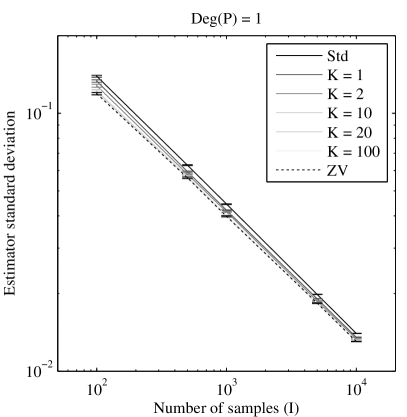
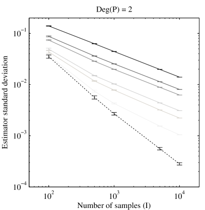
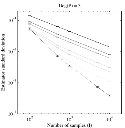
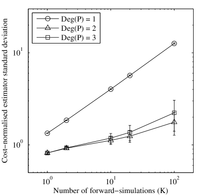
Figure 1: Tractable exponential example. Comparing the standard deviations of Monte Carlo estimators, including the default estimator (“Std”; the regular MCMC estimator with no variance reduction), the reduced-variance estimator with $K=1$, 2, 10, 20 and 100, and the ZV estimator. [The ZV estimate has some non-zero standard deviation here because, in practice, the optimal coefficients $\bm{\phi}(y)^{*}$ must be estimated using Monte Carlo.] The final panel (bottom right) displays estimator standard deviation normalised by computational cost.

All of the estimators that we consider are (essentially) unbiased (as noted before, the negligible bias resulting from estimation of $\hat{\bm{\phi}}$ can trivially be removed by data-splitting); in this section we therefore restrict attention to examining the estimator variances. The maximum variance reduction that we achieve with access to the exact score can be obtained from $\rho(\infty)=\text{Corr}_{\theta|y}(\theta,\bm{\phi}^{*}(y)^{T}\bm{m}(\theta,u))$. For degree-one polynomials $P(\theta)=a\theta$ the ZV method corresponds to $m(\theta,u)=u=-y+\frac{1}{\theta}$ and, since $\theta$ is not strongly linearly correlated with $\frac{1}{\theta}$, the maximum variance reduction that can be achieved by degree-one polynomials is not substantial. However the use of degree-two polynomials $P(\theta)=a\theta+b\theta^{2}$ leads to $\bm{m}(\theta,u)=[u,2+2\theta u]=[-y+\frac{1}{\theta},4-2y\theta]$ and taking $\bm{\phi}=[0,\frac{1}{2y}]$ leads to a control variate $\bm{\phi}^{T}\bm{m}(\theta,u)=\frac{2}{y}-\theta$. Thus the ZV estimator $g(\theta)+\bm{\phi}^{T}\bm{m}(\theta,u)$ is equal to $\frac{2}{y}$, which is independent of $\theta$, i.e. exact zero variance is achieved.

In general the score $u(\theta|y)$ will be unavailable for GRF but may be estimated by $\hat{u}(\theta|y)$ as described above, with the estimate becoming exact as $K\rightarrow\infty$. We investigate through simulation the effect of employing finite values of $K$. Intuitively the proposed approach will be more effective when the target function $g(\theta)$ of interest is strongly correlated (under the posterior) with a linear combination $\bm{\phi}^{T}\bm{m}(\theta,\hat{u})$. Fig. S1 demonstrates that when $K$ is large, the RV control variates (for degree-two polynomials) are closely correlated with the ZV control variates (left column) and, hence, with the target function $g(\theta)$ (right column). We would therefore expect to see a large reduction in Monte Carlo variance using RV estimation in this regime.

The main conclusions to be drawn from this tractable example are summarised in Fig. 1, where we display estimates for the estimator standard deviation $\text{std}[\hat{\mu}]$, computed as the standard error of the mean over all $I$ Monte Carlo samples. In total the estimation procedure was repeated 100 times and we report the mean value of $\text{std}[\hat{\mu}]$ along with the standard error of this mean computed over the 100 realisations. We considered varying the number of Monte Carlo samples $I=100,500,1000,5000,10000$, the number of forward-simulations $K=1,2,10,20,100$ and the degree of the polynomial trial function $\text{deg}(P)=1,2,3$. Results demonstrate that estimator variance reduces as either $I$ or $K$ is increased, as expected. A comparison between the plots (full data provided in Table S1) shows that degree-two polynomials considerably out-perform the degree-one polynomials, whereas the degree-three polynomials tend to slightly under-perform the degree-two polynomials. (The theoretical best ZV control variates are degree-two polynomials and therefore degree-three polynomials require that additional coefficients associated to higher order control variates - that we know, theoretically, should be equal to zero - are estimated from data, thus adding extra noise.)

To assess computational efficiency, we also report the quantity $\sqrt{IK}\text{std}[\hat{\mu}]$ that has units “standard deviation per unit serial computational cost” and can be used to evaluate the computational efficiency of competing strategies (bottom right panel of Fig. 1 and Table S1). Here we see that $K=1$ minimises $\sqrt{IK}\text{std}[\hat{\mu}]$ and is consistent with the theoretical result that $K=1$ is optimal for serial computation. Fig. S2 plots the canonical correlation coefficient between $\bm{m}(\theta,\hat{u})$ and $g(\theta)$ for values of $K=1,2,\dots,10$. Here we notice that over $80\%$ of the correlation is captured by just one forward-simulation from the likelihood ($K=1$), further supporting our theoretical result that $K=1$ is optimal for serial computation. Indeed, a theoretical prediction $\rho(K)=(K/(K+C))^{1/2}$ resulting from Lemma 5 in the Appendix, shown as a solid line in Fig. S2, closely matches these simulation results.

0.3.2 Example 2: Ising model

In the experiments below we consider an Ising model of size $n=16$, about the limit for exact solution, as defined in Sec. 0.1, Example 1, above. Assuming that the lattice points have been indexed from top to bottom in each column and that columns are ordered from left to right, then an interior point $y_{i}$ in a first order neighbourhood model has neighbours $\{y_{i-n},y_{i-1},y_{i+1},y_{i+n}\}$. Each point along the edges of the lattice has either two or three neighbours. We focus on estimating the posterior mean $\mu=\mathbb{E}_{\theta|\bm{y}}[\theta]$ under a prior $\theta\sim N(0,5^{2})$. Since the tails of the prior vanish exponentially and the likelihood is bounded, the posterior automatically satisfies the boundary conditions of Lemma 1. Here data $\bm{y}$ were simulated exactly from the likelihood using $\theta=0.4$, via the recursive scheme of Friel and Rue, (2007). This recursive algorithm also allows exact calculation of the partition function. In turn this allow a very precise estimate of the posterior mean; for the data that we consider below this posterior mean is $\mu=0.43455$, calculated numerically over a very fine grid of $\theta$ values.

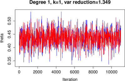
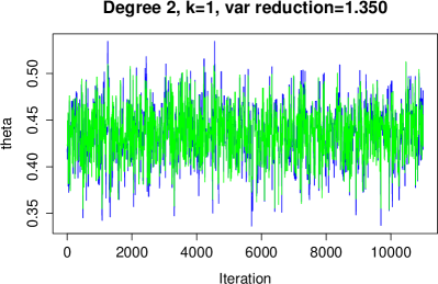
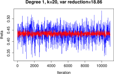
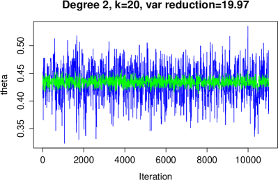
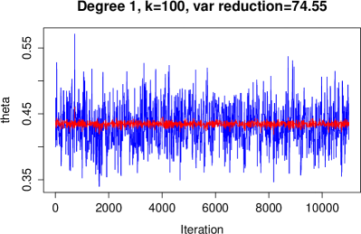
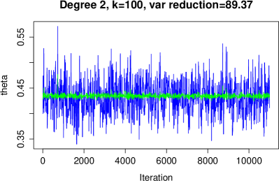
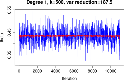
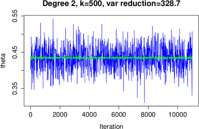
Figure 2: Ising model: As the number of forward-simulations, $K$, increases, the precision of the controlled estimate of the posterior mean for $\theta$ increases. The degree-two polynomial yields greater precision compared to the degree-one polynomial, particularly for larger values of $K$.

Fig. 2 displays the MCMC trace plots, obtained using the exchange algorithm, for $g(\theta)=\theta$ (blue) and the RV version $g(\theta)+\hat{\bm{\phi}}^{T}\bm{m}(\theta,\hat{u})$. Trace plots are presented for increasing values of $K\in\{1,20,100,500\}$ and using degree-one (red) and degree-two (green) polynomials. For $K=1$ we observe little difference between controlled (i.e. using RV control variates) and uncontrolled trajectories, suggesting that RV control variates do not justify the additional coding effort in the case of serial computation. However it is evident that as $K$ increases, the Monte Carlo variance of the controlled trajectory decreases; indeed when $K=500$ the variance is dramatically reduced compared to the (uncontrolled) MCMC samples of $\theta$. These findings are summarised in Table 1. Additionally, we find that degree-two polynomials offer a substantial improvement over degree-one polynomials in terms of variance reduction, but that this is mainly realised for larger values of $K$. These results present a powerful approach to exploit multi-core processing to deliver a real-time acceleration in the convergence of MCMC estimators.

	$K=1$	$K=20$	$K=100$	$K=500$
$\hat{\mu}$	$0.4340$	0.4345	0.4322	0.4340
$\hat{\mu}_{1}$	0.4351	0.4345	0.4347	0.4346
$\hat{\mu}_{2}$	0.4351	0.4344	0.4346	0.4346
$R=\mathbb{V}[\hat{\mu}]/\mathbb{V}[\hat{\mu}_{1}]$	1.349	18.86	74.55	187.5
$R=\mathbb{V}[\hat{\mu}]/\mathbb{V}[\hat{\mu}_{2}]$	1.350	19.97	89.37	328.7

Table 1: Ising model: As the number of forward-simulations, $K$, used to estimate the score function increases, the reduction in variance becomes more substantial. Here $\hat{\mu}$ is the standard Monte Carlo estimate, $\hat{\mu}_{1}$ is the reduced-variance estimate using degree-one polynomials and $\hat{\mu}_{2}$ is the reduced-variance estimate using degree-two polynomials. Brute-force calculation produces a value $\mu=0.43455$ for this example. [Variances were estimated with respect to empirical means.]

0.3.3 Example 3: Exponential random graph models

In the experiment below we consider the Gamaneg network (Read,, 1954), displayed in Fig. 3, that consists of $n=16$ sub-tribes of the Eastern central highlands of New Guinea. In this graph an edge represents an antagonistic relationship between two sub-tribes. Here we consider an ERG model as defined in Sec. 0.1, Example 2, with $k=2$, i.e. two sufficient statistics, where $s_{1}(y)$ counts the total number of observed edges and the two-star statistic $s_{2}(y)$ is also as defined in Sec. 0.1 above. Here the parameters $\theta_{1},\theta_{2}$ control the propensity of edges and two-star configurations, respectively, in the network. Positive values of $\theta_{1}$ and $\theta_{2}$ tend to lead to, respectively, over-representation of edges and two-star configurations in networks realised from the likelihood. The prior distributions for $\theta_{1}$ and $\theta_{2}$ were both set to be independent $N(0,5^{2})$, from which it follows that the boundary condition of Lemma 1 is satisfied. This is a benchmark dataset that has previously been used to assess Monte Carlo methodology (Friel,, 2013), making it well-suited to our purposes.

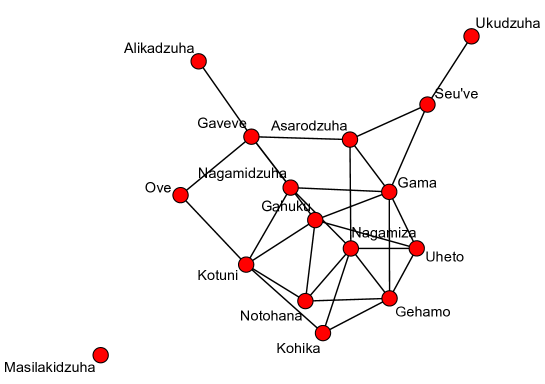
Figure 3: Gamaneg graph. The vertices represent $16$ sub-tribes of the Eastern central highlands of New Guinea and edges represent an antagonistic relationship between two sub-tribes.

Again we focus on the challenge of estimating the posterior mean $\bm{\mu}=\mathbb{E}_{\bm{\theta}|\bm{y}}[\bm{\theta}]$, in this case performing independent estimation with $g(\bm{\theta})=\theta_{j}$ for $j=1,2$. Recently Caimo and Friel, (2011), Caimo and Friel, (2014) developed Bayesian methodology for this model, based on the exchange algorithm, that can be directly utilised for the RV framework developed in this paper. The exchange algorithm was run for $I=11,000$ iterations, where at each iteration $K=500$ forward-simulations were used to estimate the score. Fig. 4 illustrates that a variance reduction of about 20 times is possible using a degree-two polynomial for each of the two components of the parameter vector. From the uncontrolled trajectories it is difficult to comment on the relative posterior means $\mu_{1}$ and $\mu_{2}$ of $\theta_{1}$ and $\theta_{2}$ respectively, but from the controlled trajectories it is visually clear that we have $\mu_{1}<\mu_{2}<0$. This suggests that posterior predictions of network structure typically contain more two-stars than edges.

We note that Caimo and Mira, (2014) recently proposed the use of delayed rejection to reduce autocorrelation in the exchange algorithm for ERG models, demonstrating an approximate two-fold variance reduction; the delayed rejection exchange algorithm is fully compatible with our methodology and, if combined, should yield a further reduction in variance.

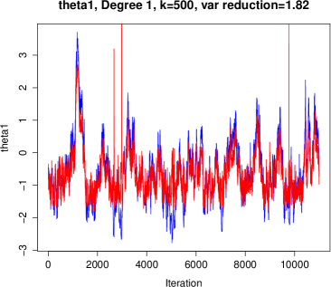
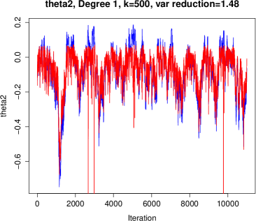
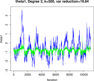
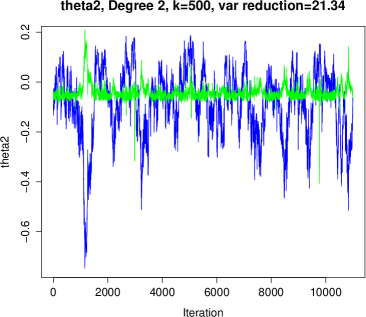
Figure 4: Exponential random graph model: The top row displays the trace plot for $\theta_{1}$ and $\theta_{2}$ in uncontrolled (blue) and controlled versions for a degree-one (red) polynomial, while the bottom row is similar but for a degree-two (green) polynomial.

0.3.4 Example 4: Nonlinear stochastic differential equations

For our final example we consider performing Bayesian inference for a system of nonlinear stochastic differential equations (SDEs) as defined in Sec. 0.1, Example 4, Eqn. 9. This problem is well-known to pose challenges for Bayesian computation and recent work in this direction includes (Beskos et al.,, 2006; Golightly and Wilkinson,, 2008). We estimate the score using

$$\nabla_{\bm{\theta}}\log p(\bm{\theta}|\bm{y})\approx\frac{1}{K}\sum_{k=1}^{K}\nabla_{\bm{\theta}}\log p(\bm{\theta},\bm{x}^{(k)}|\bm{y})$$ (52)

where $\bm{x}^{(k)}$ are independent samples from $p(\bm{x}|\bm{\theta},\bm{y})$. Such samples can be generated using MCMC techniques and in this paper we make use of a Metropolis-Hastings sampler with “diffusion bridge” proposals (Fuchs,, 2013). Note that since $p(\bm{\theta},\bm{x}|\bm{y})\propto p(\bm{y},\bm{x}|\bm{\theta})p(\bm{\theta})=p(\bm{x}|\bm{\theta})p(\bm{\theta})$, we have that

$$\nabla_{\bm{\theta}}\log p(\bm{\theta},\bm{x}|\bm{y})=\nabla_{\bm{\theta}}\log p(\bm{\theta})+\nabla_{\bm{\theta}}\log p(\bm{x}|\bm{\theta}).$$ (53)

Direct calculation shows that, assuming $\bm{\beta}$ is invertible,

$$\nabla_{\theta_{j}}\log p(\bm{X}|\bm{\theta})=\sum_{i=2}^{T}\begin{array}[]{l}-\frac{1}{2}\text{tr}(\bm{\beta}_{i}^{-1}\nabla_{\theta_{j}}\bm{\beta}_{i})+(\nabla_{\theta_{j}}\bm{\alpha}_{i})^{T}\bm{\beta}_{i}^{-1}(\bm{X}_{i}-\bm{X}_{i-1}-\bm{\alpha}_{i}\delta t)\\ \;\;\;\;\;+\frac{1}{2\delta t}(\bm{X}_{i}-\bm{X}_{i-1}-\bm{\alpha}_{i}\delta t)^{T}\bm{\beta}_{i}^{-1}(\nabla_{\theta_{j}}\bm{\beta}_{i})\bm{\beta}_{i}^{-1}(\bm{X}_{i}-\bm{X}_{i-1}-\bm{\alpha}_{i}\delta t)\end{array}$$ (56)

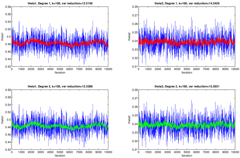
Figure 5: SIR model. The top row displays the trace plots for $\theta_{1}$ and $\theta_{2}$ in uncontrolled (blue) and controlled (red) versions for a degree-one polynomial. The bottom row is similar, but for degree-two polynomials.

Consider the specific example of the Susceptible-Infected-Recovered (SIR) model from epidemiology. Letting $X_{1}$, $X_{2}$ denote respectively the proportions of susceptible and infected individuals in a population, modelled as continuous random variables, the SIR model has a stochastic representation given by

$$\bm{\alpha}(\bm{X};\bm{\theta})=\left[\begin{array}[]{c}-\theta_{1}X_{1}X_{2}\\ \theta_{1}X_{1}X_{2}-\theta_{2}X_{2}\end{array}\right],\;\;\;\;\;\bm{\beta}(\bm{X};\bm{\theta})=\frac{1}{N}\left[\begin{array}[]{cc}\theta_{1}X_{1}X_{2}&-\theta_{1}X_{1}X_{2}\\ -\theta_{1}X_{1}X_{2}&\theta_{1}X_{1}X_{2}+\theta_{2}X_{2}\end{array}\right]$$ (61)

where $N$ is a fixed population size and the rate parameters $\bm{\theta}\in[0,\infty)^{2}$ are unknown. We assess our methodology by attempting to estimate the posterior mean of $\bm{\theta}$, taking $g(\bm{\theta})=\theta_{j}$ for $j=1,2$ in turn. Here each $\theta_{j}$ was assigned an independent Gamma prior with shape and scale hyperparameters both equal to 2. This prior vanishes at the origin and has exponentially decaying tails, so that the boundary condition of Lemma 1 is satisfied by all polynomials. Data were generated using the initial condition $\bm{X}_{0}=[0.99,0.01]$, population size $N=1,000$ and parameters $\bm{\theta}=[0.5,0.25]$. Observations were made at 20 evenly spaced intervals in the period from $t=0$ to $t=35$. Five latent data points were introduced between each observed data point, so that the latent process has dimension $2\times(20-1)\times 5=190$. At each Monte Carlo iteration we sampled $K=100$ realisations of the latent data process $\bm{X}^{u}$.

Fig. 5 demonstrates that a variance reduction of about 12-14 times is possible using degree-one polynomials and 13-15 times using degree-two polynomials. Again, these results highlight the potential to exploit multi-core processing for variance reduction in Monte Carlo methodology.

0.4 Conclusions

In this paper we have shown how repeated forward-simulation enables reduced-variance estimation in models that have intractable likelihoods. The examples that we have considered illustrate the value of the proposed methodology in spatial statistics, social network analysis and inference for latent data models such as SDEs. The RV methodology provides a straight-forward means to leverage multi-core architectures for Bayesian estimation, that compliments recent work for MCMC in this direction by Alquier et al., (2014); Angelino et al., (2014); Bardenet et al., (2014); Calderhead, (2014); Korattikara et al., (2014); Maclaurin and Adams, (2014). Our theoretical analysis revealed that the number $K$ of forward-simulations should be taken equal to the number of cores in order to provide the optimal variance reduction per unit (serial) computation. Furthermore, it was shown that the proposed RV estimator converges to the (intractable) ZV estimator of Mira et al., (2013) as the number $K$ of cores becomes infinite. Our theoretical findings are supported by empirical results on standard benchmark datasets, that demonstrate a substantial variance reduction can be realised in practice. In particular, results for the Ising model demonstrate that a 200-300 times variance reduction can be achieved by exploiting a $K=500$ core architecture. More generally, our work shows that it may not be necessary to parallelise the sampling process itself; the potential of massively multi-core architectures can be harnessed in post-processing MCMC samples using control variates.

To conclude, we suggest interesting directions for further research:

• The approach that we pursued was a post-processing procedure that does not require modification to the MCMC sampling mechanism itself. However an interesting possibility would be to also use the output of forward-sampling to construct gradient-based proposal mechanisms for the underlying MCMC sampler, following recent work in this direction by Alquier et al., (2014); Nemeth et al., (2014). This would retain the inherently parallel nature of the simulation procedure whilst yielding useful approximate Monte Carlo schemes that converge to an “idealised” (i.e. marginal) sampler as the number of forward-simulations, $K$, increases. In particular, our procedure can be implemented within the various schemes developed in Alquier et al., (2014); Nemeth et al., (2014) without any additional computational cost. Stochastic approximation of the score function was also recently considered by Atchadé et al., (2014) in the context of designing proximal gradient algorithms. Our work therefore combines to illustrate the wide range of statistical models for which such an approach could prove practically useful. Alternative approaches to handling Type I intractability, such as Approximate Bayesian Computation (Marjoram et al.,, 2003) typically also require a forward-simulation step and thus could also be embedded within our framework.

• In terms of statistical efficiency it would be interesting to extend the reduced-variance methodology to the non-parametric setting recently considered by Oates et al., (2014), that provides a mechanism to learn a suitable trial function $P(\bm{\theta})$ that need not be polynomial, leading (in some cases) to improved convergence rates. A second interesting possibility would be to allow the number of forward-simulations, $K$ to depend upon the current state $\bm{\theta}$; in this way fewer simulations could be performed when it is expected that the score estimate $\hat{\bm{u}}(\bm{\theta}|\bm{y})$ is likely to have a low variance. A third direction would be to move beyond independent estimation of the score $\bm{u}(\bm{\theta}|\bm{y})$ for each value of $\bm{\theta}$; here non-parametric regression techniques could play a role and this should yield further reductions in estimator variance, which again has a close analogy with Oates et al., (2014).

• Finally, a referee suggested the intruiging possibility to expolit control variates for reduced-variance density estimation. Specifically, we would take $g_{\bm{\theta}^{*}}(\bm{\theta})=K_{h}(\bm{\theta}^{*}-\bm{\theta})$ for a bandwidth-$h$ kernel smoother estimate for the posterior density at a point $\bm{\theta}^{*}\in\Theta$, such that $\mathbb{E}_{\bm{\theta}|\bm{y}}[g_{\bm{\theta}^{*}}(\bm{\theta})]\rightarrow p(\bm{\theta}^{*}|\bm{y})$ as $h\rightarrow 0$. This is a direction that we are keen to explore further.

Of course, in the era of big data, as statisticians are increasingly interested in analysing larger datasets an immediate challenge is the issue of dealing with intractable likelihoods, due to the volume of data. Moreover, one would anticipate that statistical methodology will focus on the development of inferential algorithms that exploit modern multi-core computer architectures. Both of these will inevitably lead to further development and extensions of the methodology described in this paper.

The authors are grateful for the constructive feedback they received from the Editors and Reviewers at Bayesian Analysis. NF was supported by the Science Foundation Ireland [12/IP/1424]. The Insight Centre for Data Analytics is supported by Science Foundation Ireland [SFI/12/RC/2289]. AM was supported by the Swiss National Science Foundation [CR12I1-156229]. CJO was supported by the EPSRC Centre for Research in Statistical Methodology [EP/D002060/1]. The authors thank Mark Girolami for helpful discussions.

Appendix

Below we prove Lemma 4 from the Main Text. First we require a technical result:

Lemma 5.

Write $\rho(\infty)=\text{\emph{Corr}}_{\bm{\theta}|\bm{y}}[g(\bm{\theta}),h(\bm{\theta}|\bm{y})]$. There exists $C\in(0,\infty)$ such that

$$\rho(K)^{2}=\left(\frac{1}{\rho(\infty)^{2}}+\frac{C}{K}\right)^{-1}.$$ (62)

Proof.

For Type I models write $\hat{h}(\bm{\theta},\bm{Y})=h(\bm{\theta})+\epsilon(\bm{\theta},\bm{Y})$ where $\bm{Y}=(\bm{Y}_{1},\dots,\bm{Y}_{K})$ and we suppress dependence on the data $\bm{y}$ in this notation. It follows that the discrepancy between the reduced-variance and ZV control variates is given by

$$\epsilon(\bm{\theta},\bm{Y})=\nabla_{\bm{\theta}}P(\bm{\theta})\cdot\left[\frac{1}{K}\sum_{k=1}^{K}\bm{s}(\bm{Y}_{k})-\mathbb{E}_{\bm{Y}^{\prime}|\bm{\theta}}[\bm{s}(\bm{Y}^{\prime})]\right].$$ (63)

Taking an analogous approach to Type II models we obtain

$$\epsilon(\bm{\theta},\bm{X})=\nabla_{\bm{\theta}}P(\bm{\theta})\cdot\left[\frac{1}{K}\sum_{k=1}^{K}\bm{u}(\bm{\theta},\bm{X}_{k})-\mathbb{E}_{\bm{X}^{\prime}|\bm{\theta},\bm{y}}[\bm{u}(\bm{\theta},\bm{X}^{\prime})]\right].$$ (64)

Note that $\mathbb{E}_{\bm{Y}|\bm{\theta}}[\epsilon(\bm{\theta},\bm{Y})]=0$ and hence

$$\mathbb{E}_{\bm{Y},\bm{\theta}|\bm{y}}[\epsilon(\bm{\theta},\bm{Y})]=\mathbb{E}_{\bm{Y}|\bm{\theta},\bm{y}}\mathbb{E}_{\bm{\theta}|\bm{y}}[\epsilon(\bm{\theta},\bm{Y})]=\mathbb{E}_{\bm{\theta}|\bm{y}}\mathbb{E}_{\bm{Y}|\bm{\theta}}[\epsilon(\bm{\theta},\bm{Y})]=0,$$ (65)

with an analogous result holding for Type II models. Using these results we have that, for Type I models

$$\mathbb{V}_{\bm{Y},\bm{\theta}|\bm{y}}[\epsilon(\bm{\theta},\bm{Y})] = \mathbb{E}_{\bm{Y},\bm{\theta}|\bm{y}}[\epsilon(\bm{\theta},\bm{Y})^{2}]$$ (66)

$$= \mathbb{E}_{\bm{\theta}|\bm{y}}\mathbb{E}_{\bm{Y}|\bm{\theta}}[\epsilon(\bm{\theta},\bm{Y})^{2}]=\mathbb{E}_{\bm{\theta}|\bm{y}}\mathbb{V}_{\bm{Y}|\bm{\theta}}[\epsilon(\bm{\theta},\bm{Y})]$$ (67)

$$= \mathbb{E}_{\bm{\theta}|\bm{y}}[K^{-1}\mathbb{V}_{\bm{Y}|\bm{\theta}}[\nabla_{\bm{\theta}}P(\bm{\theta})\cdot\bm{s}(\bm{Y})]]=C_{1}K^{-1}$$ (68)

where $C_{1}=\mathbb{E}_{\bm{\theta}|\bm{y}}\mathbb{V}_{\bm{Y}|\bm{\theta}}[\nabla_{\bm{\theta}}P(\bm{\theta})\cdot\bm{s}(\bm{Y})]$. Also observe that, for any function $g(\bm{\theta})$,

$$\text{Cov}_{\bm{Y},\bm{\theta}|\bm{y}}[g(\bm{\theta}),\epsilon(\bm{\theta},\bm{Y})] = \mathbb{E}_{\bm{Y},\bm{\theta}|\bm{y}}[g(\bm{\theta})\epsilon(\bm{\theta},\bm{Y})]-\mathbb{E}_{\bm{Y},\bm{\theta}|\bm{y}}[g(\bm{\theta})]\mathbb{E}_{\bm{Y},\bm{\theta}|\bm{y}}[\epsilon(\bm{\theta},\bm{Y})]$$ (69)

$$= \mathbb{E}_{\bm{\theta}|\bm{y}}\mathbb{E}_{\bm{Y}|\bm{\theta}}[g(\bm{\theta})\epsilon(\bm{\theta},\bm{Y})]=0.$$ (70)

Putting these results together we obtain

$$\rho(K)=\frac{\text{Cov}_{\bm{Y},\bm{\theta}|\bm{y}}[g(\bm{\theta}),\hat{h}(\bm{\theta},\bm{Y})]}{\sqrt{\mathbb{V}_{\bm{Y},\bm{\theta}|\bm{y}}[g(\bm{\theta})]}\sqrt{\mathbb{V}_{\bm{Y},\bm{\theta}|\bm{y}}[\hat{h}(\bm{\theta},\bm{Y})]}}=\frac{\text{Cov}_{\bm{\theta}|\bm{y}}[g(\bm{\theta}),h(\bm{\theta})]}{\sqrt{\mathbb{V}_{\bm{\theta}|\bm{y}}[g(\bm{\theta})]}\sqrt{\mathbb{V}_{\bm{\theta}|\bm{y}}[h(\bm{\theta})]+C_{1}K^{-1}}}$$ (71)

from which it follows that

$$\frac{1}{\rho(K)^{2}}=\frac{\mathbb{V}_{\bm{\theta}|\bm{y}}[g(\bm{\theta})](\mathbb{V}_{\bm{\theta}|\bm{\bm{Y}}}[h(\bm{\theta})]+C_{1}K^{-1})}{\text{Cov}_{\bm{\theta}|\bm{y}}[g(\bm{\theta}),h(\bm{\theta})]^{2}}=\frac{1}{\rho(\infty)^{2}}+\frac{C}{K}$$ (72)

where $C=C_{1}/\text{Cov}_{\bm{\theta}|\bm{y}}[g(\bm{\theta}),h(\bm{\theta})]^{2}$. The analogous derivation for Type II models completes the proof. ∎

A simple corollary of Lemma 5 is that the reduced-variance estimator converges to the (unavailable) ZV estimator as $K\rightarrow\infty$. Moreover we can derive an optimal choice for $K$ subject to fixed computational cost:

Proof of Lemma 4.

Starting from Eqn. 50, we substitute $I=c/\lceil K/K_{0}\rceil$ and use the identity in Lemma 5 to obtain

$$r(K)=\frac{1}{c}\bigg{\lceil}\frac{K}{K_{0}}\bigg{\rceil}\left(1-\frac{K\rho(\infty)^{2}}{K+C\rho(\infty)^{2}}\right).$$ (73)

Fig. S3 displays typical cost-normalised variance ratios $r(K)$, for both non-Gaussian (i.e. $\rho(\infty)<1$; left) and Gaussian (i.e. $\rho(\infty)=1$; right) cases. In each case it the minimum is attained at $K=K_{0}$. In general, we see from first principles that (i) $r>0$, (ii) $r(k)$ is increasing for $k=K_{0},2K_{0},3K_{0},\dots$, and (iii) $r(k)$ is decreasing on the interval $((n-1)K_{0},nK_{0}]$ and bounded below by $r((n-1)K_{0})$, for any $n\in\mathbb{N}$. Thus we have $\arg\min_{K=1,2,3,\dots}r(K)=K_{0}$, as required. ∎

References

- Augustin et al., (1996) Augustin, N., Mugglestone, M., and Buckland, S. (1996). “An autologistic model for spatial distribution of wildlife.” Journal of Applied Ecology, 33(2):339-347.
- Alquier et al., (2014) Alquier, P., Friel, N., Everitt, R., and Boland, A. (2014). “Noisy Monte Carlo: Convergence of Markov chains with approximate transition kernels.” arXiv:1403.5496.
- Andradóttir et al., (1993) Andradóttir, S., Heyman, D. P., and Teunis, J. O. (1993). “Variance reduction through smoothing and control variates for Markov Chain simulations.” ACM Transactions on Modeling and Computer Simulation (TOMACS), 3(3):167-189.
- Andrieu and Roberts, (2009) Andrieu, C., and Roberts, G. O. (2009). “The pseudo-marginal approach for efficient Monte Carlo computations.” The Annals of Statistics, 37(2):697-725.
- Andrieu et al., (2010) Andrieu, C., Doucet, A., and Holenstein, R. (2010). “Particle Markov chain Monte Carlo (with Discussion).” Journal of the Royal Statistical Society, Series B, 72(3):269-342.
- Angelino et al., (2014) Angelino, E., Kohler, E., Waterland, A., Seltzer, M., and Adams, R. P. (2014). “Accelerating MCMC via Parallel Predictive Prefetching.” arXiv:1403.7265.
- Anh et al., (2012) Ahn, S., Korattikara, A., and Welling, M. (2012). “Bayesian Posterior Sampling via Stochastic Gradient Fisher Scoring.” In Proceedings of the 29th International Conference on Machine Learning.
- Armond et al., (2014) Armond, J., Saha, K., Rana, A. A., Oates, C. J., Jaenisch, R., Nicodemi, M., Mukherjee, S. (2014). “A stochastic model dissects cellular states and heterogeneity in transition processes”. Nature Scientific Reports, 4:3692.
- Assaraf and Caffarel, (1999) Assaraf, R., and Caffarel, M. (1999), Zero-Variance Principle for Monte Carlo Algorithms. Phys. Rev. Lett. 83(23):4682–4685.
- Atchadé et al., (2014) Atchadé, Y, Fort, G., and Moulines, E. (2014). “On stochastic proximal gradient algorithms.” arXiv:1402.2365.
- Bandyopadhyay et al., (2009) Bandyopadhyay, D., Reich, B. J., and Slate, E. (2009). “Bayesian Modeling of Multivariate Spatial Binary Data with applications to Dental Caries.” Statistics in Medicine, 28(28):3492-3508.
- Bardenet et al., (2014) Bardenet, R., Doucet, A., and Holmes, C. (2014). “Towards scaling up Markov chain Monte Carlo : an adaptive subsampling approach.” In Proceedings of the 31st International Conference on Machine Learning, 405-413.
- Besag, (1972) Besag, J. E. (1972). “Nearest-neighbour systems and the auto-logistic model for binary data.” Journal of the Royal Statistical Society, Series B, 34(1):697-725.
- Besag, (1996) Besag, J. E. (1974) “Spatial interaction and the statistical analysis of lattice systems (with discussion).” Journal of the Royal Statistical Society, Series B, 36(2):192-236.
- Beskos et al., (2006) Beskos, A., Papaspiliopoulos, O., Roberts, G. O., and Fearnhead, P. (2006). “Exact and computationally efficient likelihood-based estimation for discretely observed diffusion processes (with discussion).” Journal of the Royal Statistical Society, Series B, 68(3):333-382.
- Beskos et al., (2013) Beskos, A., Kalogeropoulos, K., and Pazos, E. (2013). “Advanced MCMC methods for sampling on diffusion pathspace.” Stochastic Processes and their Applications, 123(4):1415-1453.
- Caimo and Friel, (2011) Caimo, A., and Friel, N. (2011). “Bayesian inference for exponential random graph models.” Social Networks, 33:41-55.
- Caimo and Friel, (2013) Caimo, A., and Friel, N. (2013). “Bayesian model selection for exponential random graph models.” Social Networks, 35:11-24.
- Caimo and Friel, (2014) Caimo, A., and Friel, N. (2014). “Bergm: Bayesian inference for exponential random graphs using R.” Journal of Statistical Software, 61(2).
- Caimo and Mira, (2014) Caimo, A., and Mira, A. (2014). “Efficient computational strategies for Bayesian social networks.” Statistics and Computing, to appear.
- Calderhead, (2014) Calderhead, B. (2014). “A general construction for parallelizing Metropolis-Hastings algorithms.” Proceedings of the National Academy of Sciences, USE, 111(49):17408-17413.
- Cappé et al., (2005) Cappé, O., Moulines, E., and Ryden, T. (2005). “Inference in hidden Markov models.” Springer, New York.
- Davison et al., (2012) Davison, A. C., Padoan, S. A., and Ribatet, M. (2009). “Statistical modelling of spatial extremes.” Statistical Science, 27:161-186.
- Dellaportas and Kontoyiannis, (2012) Dellaportas, P., and Kontoyiannis, I. (2012). “Control variates for estimation based on reversible Markov chain Monte Carlo samplers.” Journal of the Royal Statistical Society, Series B, 74(1):133-161.
- Doucet et al., (2012) Doucet, A., Pitt, M., Deligiannidis, G., and Kohn, R. (2012). “Efficient implementation of Markov chain Monte Carlo when using an unbiased likelihood estimator.” arXiv:1210.1871.
- Evans and Swartz, (2000) Evans, M., and Swartz, T. (2000). “Approximating integrals via Monte Carlo and deterministic methods.” Oxford University Press.
- Everitt, (2012) Everitt, R. (2012). “Bayesian parameter estimation for latent Markov random fields and social networks.” Journal of Computational and graphical Statistics. 21(4):940-960.
- Fahrmeir and Lang, (2001) Fahrmeir, L., and Lang, S. (2001). “Bayesian inference for generalized additive mixed models based on Markov random field priors.” Journal of the Royal Statistical Society, Series C, 50(2):201-220.
- Friel and Rue, (2007) Friel, N., and Rue, H. (2007). “Recursive computing and simulation-free inference for general factorizable models.” Biometrika, 94:661-672.
- Friel, (2013) Friel, N. (2013). “Estimating the evidence for Gibbs random fields.” Journal of Computational and Graphical Statistics, 22:518-532.
- Fuchs, (2013) Fuchs, C. (2013). Inference for Diffusion Processes with Applications in Life Sciences. Springer, Heidelberg.
- Glasserman, (2004) Glasserman, P. (2004). Monte Carlo methods in financial engineering. Springer, New York.
- Golightly and Wilkinson, (2008) Golightly, A., and Wilkinson, D. J. (2008). “Bayesian inference for nonlinear multivariate diffusion models observed with error.” Computational Statistics and Data Analysis, 52(3):1674-1693.
- Geyer and Thompson, (1992) Geyer, C. J., and Thompson, E. A. (1992). “Constrained Monte Carlo maximum likelihood for dependent data (with discussion).” Journal of the Royal Statistical Society, Series B, 54(3):657-699.
- Hammer and Tjelmeland, (2008) Hammer, H., and Tjelmeland, H. (2008). “Control variates for the Metropolis-Hastings algorithm.” Scandinavian Journal of Statistics 35(3):400-414.
- He et al., (2009) He, F., Zhou, J., and Zhu, H. (2003). “Autologistic regression model for the distribution of vegetation.” Journal of Agricultural, Biological, and Environmental Statistics, 8(2):205-222.
- Huffer and Wu, (1998) Huffer, F. W., and Wu, H. (1998). “Markov Chain Monte Carlo for Autologistic Regression Models with Application to the Distribution of Plant Species.” Biometrics, 54:509-524.
- Kendall and Bourne, (1992) Kendall, P. C., and Bourne, D. E. (1992). “Vector analysis and Cartesian tensors (3rd ed.).” CRC Press, Florida.
- Korattikara et al., (2014) Korattikara, A., Chen, Y., and Welling, M. (2014). “Austerity in MCMC Land: Cutting the Metropolis-Hastings Budget.” In Proceedings of the 31st International Conference on Machine Learning, 181-189.
- Kou et al., (2012) Kou, S. C., Olding, B. P., Lysy, M., and Liu, J. S. (2012). “A multiresolution method for parameter estimation of diffusion processes.” Journal of the American Statistical Association, 107(500):1558-1574.
- Lamberton and Lapeyre, (2007) Lamberton, D., and Lapeyre, B. (2007). Introduction to stochastic calculus applied to finance. CRC Press.
- Lee et al., (2010) Lee, A., Yau, C., Giles, M., Doucet, A., and Holmes, C. (2010). “On the utility of graphics cards to perform massively parallel simulation of advanced Monte Carlo methods.” Journal of Computational and Graphical Statistics 19(4):769-789.
- Lindgren et al., (2011) Lindgren, F., Rue, H., and Lindstr’́om, J. (2011). “An explicit link between Gaussian fields and Gaussian Markov random fields: the stochastic partial differential equation approach.” Journal of the Royal Statistical Society, Series B, 73(4):423-498.
- Lyne et al., (2013) Lyne, A. M., Girolami, M., Atchade, Y., Strathmann, H., and Simpson, D. (2013). “Playing Russian Roulette with Intractable Likelihoods.” arXiv:1306.4032.
- Marjoram et al., (2003) Marjoram, P., Molitor, J., Plagnol, V., and Tavaré, S. (2003). “Markov chain Monte Carlo without likelihoods.” Proceedings of the National Academy of Sciences, U.S.A., 100:15324-15328.
- Maclaurin and Adams, (2014) Maclaurin, D., and Adams, R. P. (2014). “Firefly Monte Carlo: Exact MCMC with Subsets of Data.” In Proceedings of the 30th Annual Conference on Uncertainty in Artificial Intelligence, 543-552.
- Mira et al., (2001) Mira, A., Möller, J., and Roberts, G. O. (2001). “Perfect Slice Samplers.” Journal of the Royal Statistical Society, Series B, 63(3):593-606.
- Mira et al., (2003) Mira, A., Tenconi, P., and Bressanini, D. (2003). “Variance reduction for MCMC.” Technical Report 2003/29, Universitá degli Studi dell’ Insubria, Italy.
- Mira et al., (2013) Mira, A., Solgi, R., and Imparato, D. (2013). “Zero Variance Markov Chain Monte Carlo for Bayesian Estimators.” Statistics and Computing 23(5):653-662.
- Møller et al., (2006) Møller, J., Pettitt, A. N., Reeves, R, and Berthelsen, K. K. (2006). “An efficient Markov chain Monte Carlo method for distributions with intractable normalising constants.” Biometrika, 93:451-458.
- Murray et al., (2006) Murray, I., Ghahramani, Z., and MacKay, D. (2006). “MCMC for doubly-intractable distributions.” In Proceedings of the 22nd Annual Conference on Uncertainty in Artificial Intelligence, 359-366.
- Nemeth et al., (2014) Nemeth, C., Sherlock, C., and Fearnhead, P. (2014). “Particle Metropolis adjusted Langevin algorithms.” arXiv:1412.7299.
- Oates et al., (2014) Oates, C. J., Girolami, M., and Chopin, N. (2014). “Control functionals for Monte Carlo integration.” CRiSM Working Paper, The University of Warwick, 14:22.
- Oates et al., (2015) Oates, C. J., Papamarkou, T., and Girolami, M. (2015). “The Controlled Thermodynamic Integral for Bayesian Model Comparison.” Journal of the American Statistical Association, to appear.
- Øksendal, (2003) Øksendal, B. (2003). “Stochastic differential equations.” Springer-Verlag, Berlin.
- Papamarkou et al., (2014) Papamarkou, T., Mira, A., and Girolami, M. (2014). “Zero Variance Differential Geometric Markov Chain Monte Carlo Algorithms.” Bayesian Analysis, 9(1):97-128.
- Papamarkou et al., (2015) Papamarkou, T., Mira, A., and Girolami, M. (2015). “Hamiltonian Methods and Zero-Variance Principle.” In: Current Trends in Bayesian Methodology with Applications (eds. Dipak K. Dey, Umesh Singh and A. Loganathan), Chapman and Hall/CRC Press.
- Pillai and Smith, (2014) Pillai, N. S., and Smith, A. (2014) “Ergodicity of Approximate MCMC Chains with Applications to Large Data Sets.” arXiv:1405.0182.
- Potamianos and Goutsias, (1997) Potamianos, G., and Goutsias, J. (1997). “Stochastic approximation algorithms for partition function estimation of Gibbs random fields.” IEEE Transactions on Information Theory, 43(6):1948-1965.
- Propp and Wilson, (1996) Propp, J. G., and Wilson, D. B. (1996). “Exact sampling with coupled Markov chains and applications to statistical mechanics.” Random Structures and Algorithms, 9(1):223-252.
- Read, (1954) Read, K. E. (1954). “Cultures of the Central Highlands, New Guinea.” Southwestern Journal of Anthropology 10(1):1-43.
- Robins et al., (2014) Robins, G., Pattison, P., Kalish, Y., and Lusher, D. (2007). “An introduction to exponential random graph models for social networks.” Social Networks, 29:173-191.
- Rubinstein and Marcus, (1985) Rubinstein, R. Y., and Marcus, R. (1985). “Efficiency of Multivariate Control Variates in Monte Carlo Simulation.” Operations Research, 33(3):661-677.
- Rue et al., (2009) Rue, H., Martino, S., and Chopin, N. (2009). “Approximate Bayesian inference for latent Gaussian models by using integrated nested Laplace approximations (with discussion).” Journal of the Royal Statistical Society, Series B, 71(2):319-392.
- Sherlock et al., (2014) Sherlock, C., Thiery, A., Roberts, G. O., and Rosenthal, J. S. (2014). “On the efficiency of pseudo-marginal random walk Metropolis algorithm.” The Annals of Statistics, to appear.
- Suchard et al., (2010) Suchard, M., Wang, Q., Chan, C., Frelinger, J., Cron, A., and West, M. (2010). “Understanding GPU programming for statistical computation: Studies in massively parallel massive mixtures.” Journal of Computational and Graphical Statistics 19(2):419-438.
- Welling and Teh, (2011) Welling, M., and Teh, Y. W. (2011). “Bayesian Learning via Stochastic Gradient Langevin Dynamics.” In Proceedings of the 28th International Conference on Machine Learning, 681-688.
- West and Harrison, (1997) West, M., and Harrison, J. (1997). Bayesian Forecasting and Dynamic Models (2nd ed.). Springer-Verlag, New York.
- Wilkinson, (2011) Wilkinson, D. J. (2011). Stochastic Modelling for Systems Biology. CRC Press.