Quadrupole Shifts for the ¹⁷¹Yb⁺ Ion Clocks: Experiments versus Theories

Abstract

Quadrupole shifts for three prominent clock transitions, $[4f^{14}6s]^{2}S_{1/2}\rightarrow[4f^{14}5d]^{2}D_{3/2}$, $[4f^{14}6s]^{2}S_{1/2}\rightarrow[4f^{14}5d]^{2}D_{5/2}$ and $[4f^{14}6s]^{2}S_{1/2}\rightarrow[4f^{13}6s^{2}]^{2}F_{7/2}$, in the Yb⁺ ion are investigated by calculating the quadrupole moments ($\Theta$s) of the $5d_{3/2,5/2}$ and $4f_{7/2}$ states using the relativistic coupled-cluster (RCC) methods. We find an order difference in the $\Theta$ value of the $4f_{7/2}$ state between our calculation and the experimental result, but our result concur with the other calculations that are carried out using different many-body methods than ours. However, our $\Theta$ value of the $5d_{3/2}$ state is in good agreement with the available experimental result and becomes more precise till date to estimate the the quadrupole shift of the $[4f^{14}6s]^{2}S_{1/2}\rightarrow[4f^{14}5d]^{2}D_{3/2}$ clock transition more accurately. To justify the accuracies in our calculations, we evaluate the hyperfine structure constants of the $6s_{1/2}$, $5d_{3/2,5/2}$ and $4f_{7/2,5/2}$ states of ¹⁷¹Yb⁺ ion using the same RCC methods and compare the results with their experimental values. We also determine the lifetime of the $5d_{3/2}$ state to eradicate the scepticism on the earlier measured value as claimed by a recent experiment.

A single trapped Al⁺ ion is the most accurate atomic clock till date chou1 implying that one of the singly charged ions is capable of becoming the primary frequency standard in future provided its stability can be further improved. The other successful optical single ion clocks are Hg⁺ oskay , Ca⁺ matsubara , Sr⁺ margolis , Yb⁺tamm ; roberts etc. In Yb⁺, two quadrupole (E2) $[4f^{14}6s]^{2}S_{1/2}\rightarrow[4f^{14}5d]^{2}D_{3/2}$ and $[4f^{14}6s]^{2}S_{1/2}\rightarrow[4f^{14}5d]^{2}D_{5/2}$ transitions having optical wavelengths 436 nm and 411 nm, respectively, and an octupole (E3) $[4f^{14}6s]^{2}S_{1/2}\rightarrow[4f^{13}6s^{2}]^{2}F_{7/2}$ transition with optical wavelength 467 nm are considered for the clock measurements, see Fig. 1, in many laboratories around the globe tamm ; roberts ; imai ; subha . Since the field-induced frequency shifts in the $[4f^{13}6s^{2}]^{2}F_{7/2}$ state is very low and it is also highly meta-stable huntemann , it makes the above octupole transition as an instinctive choice to think as the most precise and stable next genre optical clock. Although the lifetime of the $[4f^{13}6s^{2}]^{2}F_{7/2}$ state is very long ($>$ 6 years) which cannot be considered as the interrogation time during the clock frequency measurement, instead its probe interaction time ($\sim$ 10 s) serves this purpose huntemann . On the otherhand, the lifetimes of the metastable $[4f^{14}5d]^{2}D_{3/2}$ and $[4f^{14}5d]^{2}D_{5/2}$ states are about 55 $ms$ and 7 $ms$, respectively yu ; schacht and can be used as the interrogation times in the clock transitions involving these states. Owing to these facts, many other important studies like parity nonconservation bijaya1 ; rahaman , quantum information olmschenk , variation of the fine structure constant godun etc. using the above transitions in Yb⁺ are also in progress.

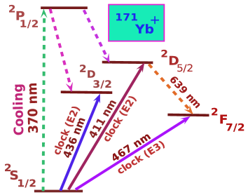
Figure 1: (color online) Schematic view of the energy levels and the clock transitions in the ¹⁷¹Yb⁺ ion.

One of the major resources that contribute to the uncertainty budget of a clock frequency measurement is the quadrupole shift resulting from the stray electric field gradient $({\bf\nabla E^{(2)}})$ during the experiment itano1 . This shift can be accurately estimated with the precise knowledge of the quadrupole moments $(\Theta$s) of the states involved in a clock transition. This urges for determination of $\Theta$s for the $[4f^{14}5d]^{2}D_{3/2}$, $[4f^{14}5d]^{2}D_{5/2}$ and $[4f^{13}6s^{2}]^{2}F_{7/2}$ states ($\Theta$ is zero for the $[4f^{14}6s]^{2}S_{1/2}$ state) of Yb⁺ as accurately as possible. In an experiment, $\Theta$ is measured by altering static direct current (dc) voltage and is very difficult to obtain very precisely. The rationale to carry out the theoretical studies of this property are: (i) when the experimental results are not available, the calculated values can be helpful to estimate the quadrupole shifts, (ii) it can prevent performing auxiliary measurements for the atomic clock experiments which are very expensive and (iii) comparison between the measurement and a calculation serves as a tool to test the potential of the employed many-body method. Thus, calculations of $\Theta$s in Yb⁺ seem to be indispensable. The previous calculations for $\Theta$s in Yb⁺ are reported as 2.174 $ea_{0}^{2}$ itano and 2.157 $ea_{0}^{2}$ latha against the measured value 2.08(11) $ea_{0}^{2}$ schneider for the $[4f^{14}5d]^{2}D_{3/2}$ state and for the $[4f^{13}6s^{2}]^{2}F_{7/2}$ state the calculated values are $-0.22\ ea_{0}^{2}$ blythe and $-0.20\ ea_{0}^{2}$ porsev compared to the measured value $-$0.041(5)$ea_{0}^{2}$ huntemann . Latha et al. latha had employed the relativistic coupled-cluster (RCC) method while Itano itano had used a multi-configuration Dirac-Fock (MCDF) method to calculate these quantities. For the $[4f^{13}6s^{2}]^{2}F_{7/2}$ state, Blythe et al. blythe had employed the MCDF method, while Porsev et al. porsev report their result inconclusively using a CI method and predicting the final value as $\sim-0.1\ ea_{0}^{2}$. In this Letter, we intend to perform calculations of $\Theta$s of these states including their fine structure partners $[4f^{14}5d]^{2}D_{5/2}$ and $[4f^{13}6s^{2}]^{2}F_{5/2}$ states by considering all possible configurations within the singles and doubles approximation in our recently developed yashpal ; nandy RCC (CCSD) methods. These methods are suppose to be more accurate than the truncated CI or MCDF methods on the physical grounds szabo ; bartlett , hence we may possibly apprehend the role of the electron correlations better in the determination of $\Theta$s and to elucidate plausible reasons for the discrepancies between the theoretical and experimental results. In addition, we calculate the magnetic dipole hyperfine constants ($A_{hf}$s) of the above states of ¹⁷¹Yb⁺ and compare them against their experimental values to gain insights into the accuracies of our calculations. Furthermore, we determine the lifetime of the $[4f^{14}5d]^{2}D_{3/2}$ state to eradicate the conflict about its correct value which is given differently by two separate measurements yu ; schacht .

Table 1: Contributions from the CCSD methods (after dividing by the corresponding normalization factors) and comparison between the other available results of the quadrupole moments ($\Theta$s) in $ea_{0}^{2}$ and the magnetic dipole hyperfine structure constants ($A_{hf}$s) in MHz of the low-lying states relevant to the clock transitions in ¹⁷¹Yb⁺. Error bars are given within the parentheses.

RCC	$4f^{13}6s^{2}\ {}^{2}F_{7/2}$		$4f^{13}6s^{2}\ {}^{2}F_{5/2}$		$4f^{14}6s\ ^{2}S_{1/2}$	$4f^{14}5d\ ^{2}D_{3/2}$		$4f^{14}5d\ ^{2}D_{5/2}$
term
	$\Theta$	$A_{hf}$	$\Theta$	$A_{hf}$	$A_{hf}$	$\Theta$	$A_{hf}$	$\Theta$	$A_{hf}$
DF	-0.2593	867.66	-0.2097	1634.09	7225.45	2.440	283.04	3.613	108.08
$\overline{O}$-DF	-0.0344	7.533	-0.0255	8.941	2490.30	-0.005	1.95	-0.008	1.10
$\overline{O}\Omega_{1}$	0.0	0.0	0.0	0.0	427.91	-0.369	64.30	-0.550	24.75
$\overline{O}\Omega_{2}$	0.0923	25.23	0.0715	87.47	2334.97	-0.021	15.87	-0.026	-207.64
$\Omega_{1}^{\dagger}\overline{O}\Omega_{1}$	0.0	0.0	0.0	0.0	4.90	0.046	4.61	0.055	1.54
$\Omega_{1}^{\dagger}\overline{O}\Omega_{2}$	0.0	0.0	0.0	0.0	-9.89	0.0003	3.70	-0.0002	-13.61
$\Omega_{2}^{\dagger}\overline{O}\Omega_{2}$	-0.0142	104.17	-0.0134	183.78	235.36	-0.023	27.60	0.032	16.78
Final	-0.216(20)	1004(100)	-0.177(50)	1914(166)	12709(400)	2.068(12)	401(14)	3.116(15)	-69(6)
Others	-0.22a				13091b	2.174c	489b	3.244c	-96b
	-0.20b					2.157d	400.48c		-12.58c
Expt.	-0.041(5)f	905.0(5)g			12645h	2.08(11)i	430(43)j		-63.6(5)k

^ablythe , ^bporsev , ^citano , ^dlatha , ^ebijaya1 , ^fhuntemann , ^gtaylor , ^hmartensson , ⁱschneider , ^jengelke , ^kroberts2

Theoretically quadrupole moment of a hyperfine state, $|(\gamma IJ)FM_{F}\rangle$, with the angular momentum $F$ and azimuthal component $M_{F}$ for the nuclear spin $I$, atomic angular momentum $J$ and $\gamma$ representing other additional information of the state is given by $\Theta(\gamma F)=\langle(\gamma IJ)FF|\Theta^{(2)}_{0}|(\gamma IJ)FF\rangle$ with $\Theta^{(2)}_{0}=-\frac{e}{2}\sum_{j}(3z^{2}_{j}-r^{2}_{j})$, the zeroth component of the quadrupole moment spherical tensor ${\bf\Theta^{(2)}}$ angel , for which we can express itano1

$$\langle(\gamma IJ)FM_{F}|\Theta^{(2)}_{q}|(\gamma IJ)FM_{F}\rangle = (-1)^{F-M_{F}}$$

$$\times\left(\begin{matrix}F&2&F\cr M_{F}&q&-M_{F}\cr\end{matrix}\right) \times \langle F||{\bf\Theta^{(2)}}||F\rangle,$$ (1)

where $\langle F||{\bf\Theta^{(2)}}||F\rangle$ is the reduced matrix element and in the $IJ$-coupling approximation it is given by

$$\langle F||{\bf\Theta^{(2)}}||F\rangle = (-1)^{I+J+F}(2F+1)\left\{\begin{matrix}J&2&J\cr F&I&F\cr\end{matrix}\right\}$$ (2)

$$\times\left(\begin{matrix}J&2&J\cr J&0&-J\cr\end{matrix}\right)^{-1}\Theta(\gamma J)$$

for $\Theta(\gamma J)=\langle JJ|\Theta^{(2)}_{0}|JJ\rangle$ the quadrupole moment of the atomic state. The quadrupole shift in the $|(\gamma IJ)FM_{F}\rangle$ state due to the interaction Hamiltonian $H_{Q}={\bf\nabla E^{(2)}\cdot\Theta^{(2)}}$ is given by itano1 ; brown

$$h\delta\nu_{Q} = \frac{-2[3M_{F}^{2}-F(F+1)]A\langle F||{\bf\Theta^{(2)}}||F\rangle}{[(2F+3)(2F+2)2F(2F-1)]^{1/2}}$$ (3)

$$\times [(3\text{cos}^{2}\beta-1)-\epsilon\ \text{sin}^{2}\beta(\text{cos}^{2}\alpha-\text{sin}^{2}\alpha)],\ \ \ \$$

where $\alpha$ and $\beta$ are the Euler angles used to convert the principal-axis frame to the laboratory frame, $\epsilon$ is known as the asymmetry parameter and $A$ is the strength of the field gradient of the applied dc voltage.

Also, the $A_{hf}$ of the $|(\gamma IJ)FM_{F}\rangle$ state is given by charles

$$A_{hf}=\mu_{N}g_{I}\frac{\langle J||T_{e}^{(1)}||J\rangle}{\sqrt{J(J+1)(2J+1)}}$$ (4)

where $g_{I}$ and $\mu_{N}$ are the gyromagnetic ratio and magnetic moment of the atomic nucleus and $T_{e}^{(1)}$ is the even parity tensor of rank one representing the electronic component of the hyperfine interaction Hamiltonian.

The lifetime of the $[4f^{14}5d]^{2}D_{3/2}$ state ($\tau_{5d3/2}$) of Yb⁺ can be determined as

$$\tau_{5d3/2}=\frac{1}{A_{5d3/2\rightarrow 6s}^{M1}+A_{5d3/2\rightarrow 6s}^{E2}},$$ (5)

where $A_{5d3/2\rightarrow 6s}^{M1}$ and $A_{5d3/2\rightarrow 6s}^{E2}$ are the transition probabilities from the $[4f^{14}5d]^{2}D_{3/2}$ state to the ground $[4f^{14}6s]^{2}S_{1/2}$ state due to the magnetic dipole (M1) and electric quadrupole (E2) transitions, respectively.

We consider the Dirac-Coulomb (DC) Hamiltonian to calculate the atomic wave functions which is given in the atomic unit (au) by

$$H = \sum_{i}[c\mbox{\boldmath$\alpha$}_{D}\cdot\textbf{p}_{i}+(\beta_{D}-1)c^{2}+V_{n}(r_{i})+\sum_{j\geq i}\frac{1}{r_{ij}}],\ \ \$$ (6)

where $\mbox{\boldmath$\alpha$}_{D}$ and $\beta_{D}$ are the Dirac matrices, $c$ is the velocity of light and $V_{n}(r)$ is the nuclear potential. The considered $[4f^{14}6s]^{2}S_{1/2}$, $[4f^{14}5d]^{2}D_{3/2,5/2}$ and $[4f^{13}6s^{2}]^{2}F_{7/2,5/2}$ states have the open-shell configurations, describing them using a common reference state in the the Fock-space formalism of the RCC theory is strenuous. For this reason, we construct two reference states, $|\Phi_{0}^{N-1}\rangle$ and $|\Phi_{0}^{N+1}\rangle$, using the Dirac-Fock (DF) method for the configurations $[4f^{14}]$ and $[4f^{14}6s^{2}]$, respectively, with $N(=69)$ as the total number of electrons to calculate the above states. Here the $[4f^{14}6s]^{2}S_{1/2}$ and $[4f^{14}5d]^{2}D_{3/2,5/2}$ states can be determined using $|\Phi_{0}^{N-1}\rangle$ by attaching the respective valence electron $v$ (denoted by $|\Psi_{v}\rangle$) and again the $[4f^{14}6s]^{2}S_{1/2}$ state and the $[4f^{13}6s^{2}]^{2}F_{7/2,5/2}$ states can be evaluated from $|\Phi_{0}^{N+1}\rangle$ by annihilating the respective extra electron $a$ (denoted by $|\Psi_{a}\rangle$). The point to be noted here is that the $[4f^{14}6s]^{2}S_{1/2}$ state obtained from $|\Phi_{0}^{N-1}\rangle$ and from $|\Phi_{0}^{N+1}\rangle$ see different DF potentials. Consequently, the difference in the results of this state when calculated using $|\Psi_{v}\rangle$ and $|\Psi_{a}\rangle$ at the same level of approximations may be able to entail the effect of the $6s$ electron in the construction of the occupied orbitals.

In the Fock-space RCC formalism, only brief discussions are given here from the detailed descriptions of Refs. yashpal ; nandy ; sahoo , we express

$$|\Psi_{v}\rangle=e^{T^{N-1}+S_{v}}a_{v}^{\dagger}|\Phi_{0}^{N-1}\rangle=e^{T^{N-1}}\{1+S_{v}\}|\Phi_{v}\rangle$$ (7)

and

$$|\Psi_{a}\rangle=e^{T^{N+1}+R_{a}}a_{a}|\Phi_{0}^{N+1}\rangle=e^{T^{N+1}}\{1+R_{a}\}|\Phi_{a}\rangle,$$ (8)

where $T^{N-1}$ and $T^{N+1}$ excite the core electrons from the new reference states $|\Phi_{v}\rangle$ and $|\Phi_{a}\rangle$, respectively, to account for the electron correlation effects and the $S_{v}$ operator annihilates the valence electron $v$ that was appended by $a_{v}^{\dagger}$ and creates a virtual orbital along with carrying out excitations of the core electrons from $|\Phi_{0}^{N-1}\rangle$ while the $R_{a}$ operator regenerates the core electron $a$ by annihilating another core electron elsewhere along with creating excitations of other core electrons from $|\Phi_{0}^{N+1}\rangle$. As was mentioned before, the core orbitals of $|\Phi_{0}^{N-1}\rangle$ do not see the interaction with the valence electron $v$. This effect along with the core-valence correlations are accounted through the contraction of $T^{N-1}$ and $\{1+S_{v}\}a_{v}^{\dagger}$. Analogously, the core electrons of $|\Phi_{0}^{N+1}\rangle$ see an extra effect from the spin pairing partner of $a$ which are removed through the product of $T^{N+1}$ and $\{1+R_{a}\}a_{a}$. Obviously, the core orbitals of $|\Phi_{0}^{N+1}\rangle$ are more relaxed here. The singles and doubles excitations in the CCSD methods are denoted by defining $T^{L}=T_{1}^{L}+T_{2}^{L}$ with $L=N-1$ and $L=N+1$ for the attachment and detachment cases, respectively, $S_{v}=S_{1v}+S_{2v}$ and $R_{a}=R_{1a}+R_{2a}$. Contributions from the important triples are estimated perturbatively nandy ; sahoo by contracting the DC Hamiltonian with $T_{2}^{N-1}$ and $S_{2v}$ in the electron attachment procedure and with $T_{2}^{N+1}$ and $R_{2a}$ in the detachment approach to account as the uncertainties due to the neglected triples.

The matrix element of a physical operator $O$ between the $|\Psi_{f}\rangle$ and $|\Psi_{i}\rangle$ states (or the expectation value with $|\Psi_{f}\rangle=|\Psi_{i}\rangle$) are determined in our RCC method by

$$\frac{\langle\Psi_{f}|O|\Psi_{i}\rangle}{\sqrt{\langle\Psi_{f}|\Psi_{f}\rangle\langle\Psi_{i}|\Psi_{i}\rangle}} = \frac{\langle\Phi_{f}|\{1+\Omega_{f}^{\dagger}\}\overline{O}\{1+\Omega_{i}\}|\Phi_{i}\rangle}{\sqrt{{\cal{N}}_{f}{\cal{N}}_{i}}},\ \ \$$ (9)

where $\overline{O}=e^{T^{L\dagger}}Oe^{T^{L}}$ and ${\cal N}_{i}=(1+\Omega_{i}^{\dagger})\overline{\cal{N}}(1+\Omega_{i})$ with $\overline{\cal N}=e^{T^{L\dagger}}e^{T^{L}}$ and $\Omega_{i}$ is either $S_{i}$ for $L=N-1$ or $R_{i}$ for $L=N+1$. Evaluation procedures of these expressions are described elsewhere nandy ; sahoo .

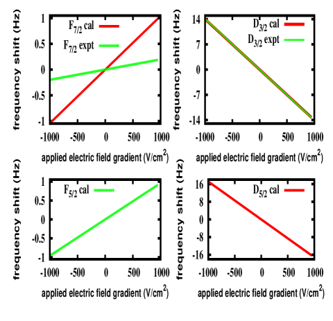
Figure 2: (color online) Quadrupole frequency shifts of the $[4f^{14}5d]^{2}D_{3/2}(F=2)$, $[4f^{14}5d]^{2}D_{5/2}(F=2)$, $[4f^{13}6s^{2}]^{2}F_{7/2}(F=3)$ and $[4f^{13}6s^{2}]^{2}F_{5/2}(F=3)$ hyperfine states for $M_{F}=0$ with respect to the $[4f^{14}6s]^{2}S_{1/2}(F=0)$ state against the electric field gradient $A$ using the calculated and measured $\Theta$ values.

In Table 1, we present $\Theta(\gamma J)$ values for all the considered states of ¹⁷¹Yb⁺ from our calculations and others along with the $A_{hf}$ results and compare them with the available measurements. We also give contributions from the DF method and from the individual CCSD (including complex conjugate (c.c.)) terms along with the estimated upper-bounds to the uncertainties within the parentheses in the same table. As seen, our final $\Theta$ values are almost in agreement with the other calculations and experimental results and also more precise, except for the $\Theta$ value of the $[4f^{13}6s^{2}]^{2}F_{7/2}$ state. Although the calculations of Ref. latha are carried out using the similar method as ours, but in the present work we have used a self-consistent procedure to account for the contributions from the non-truncative $\overline{O}$ series in contrast to Ref. latha , in which the terms are terminated at finite number of $T^{N-1}$ operators. Our $A_{hf}$ results seem to be agreeing with the experimental values within their reported error bars, which are determined using $g_{I}=0.98734$ stone . The result for the $[4f^{14}6s]^{2}S_{1/2}$ state is given only from the electron detachment method in the table. We obtain this result as 13234(900) MHz using the attachment method, which along with the $A_{hf}$s of the $[4f^{14}5d]^{2}D_{3/2,5/2}$ states are improved over our previously reported results bijaya1 due to consideration of the above self-consistent procedure and larger basis set. We find the difference between the results of the $[4f^{14}6s]^{2}S_{1/2}$ state from the two approaches, that we have considered, are very significant and the detachment theory gives more accurate result. Agreement between our $A_{hf}$ result of the $[4f^{13}6s^{2}]^{2}F_{7/2}$ state with its experimental value implies that this method is able to provide the wave functions with sufficient accuracy indicating that its $\Theta$ value is of similar accuracy. Therefore, the large differences between the theoretical and experimental results of the $[4f^{13}6s^{2}]^{2}F_{7/2}$ state $\Theta$ values are not understandable evidently. Our intuitive guess is that this discrepancy could emanate, plausibly, from some unpredictable contributions arising through the triples or other higher excitations although such signatures were obscured in our study. Its value for the hyperfine $[4f^{13}6s^{2}]^{2}F_{7/2}(F=3)$ state, in which the actual measurement has been performed, yields as $-0.19(2)$ $ea_{0}^{2}$. This value is almost same with the atomic state $\Theta$ value and again far away from $-0.041(5)$ $ea_{0}^{2}$ to possibly presume that it corresponds to the hyperfine state. This, therefore, calls for another experimental verification and more rigorous theoretical studies including higher level excitations to expunge the above ambiguity. Moreover, we also give the $\Theta$ of the fine structure partner, $[4f^{13}6s^{2}]^{2}F_{5/2}$, of the above state so that its value can be independently probed by other methods in order to cross-check our calculations. Considering our calculated $\Theta$ values for all the states, we plot in Fig. 2 the quadrupole frequency shifts ($\delta\nu$) of the $[4f^{14}5d]^{2}D_{3/2}(F=2)$, $[4f^{14}5d]^{2}D_{5/2}(F=2)$, $[4f^{13}6s^{2}]^{2}F_{7/2}(F=3)$ and $[4f^{13}6s^{2}]^{2}F_{5/2}(F=3)$ hyperfine states for $M_{F}=0$ with respect to the $[4f^{14}6s]^{2}S_{1/2}(F=0)$ state against different $A$ values and compare them with the results estimated using the available experimental $\Theta$ values. These results can be used to reduce the uncertainties in the clock transitions of Yb⁺ and for the further experimental investigations.

We also obtain M1 and E2 line strengths as $2.5\times 10^{-7}$ au and $110.25$ au, respectively, for the $[4f^{14}5d]^{2}D_{3/2}\rightarrow[4f^{14}6s]^{2}S_{1/2}$ transition from our calculations. Combining these values with the experimental energies, it yields $A_{5d3/2\rightarrow 6s}^{M1}=2.07\times 10^{-5}$ $s^{-1}$ and $A_{5d3/2\rightarrow 6s}^{E2}=19.70$ $s^{-1}$. Using these results, we get $\tau_{5d3/2}=50.78(50)$ $ms$ which is in very good agreement with the experimental result $52.7(2.4)$ $ms$ of Ref. yu and repudiate the argument by the latest experiment, which observes $\tau_{5d3/2}=61.8(6.4)$ $ms$ schacht , about underestimate of the systematics in the former measurement yu .

We acknowledge PRL 3TFlop HPC cluster for carrying out the computations.

References

- (1) C. W. Chou et al., Phys. Rev. Lett. 104, 070802 (2010).
- (2) W. H. Oskay et al., Phys. Rev. Lett. 97, 020801 (2006).
- (3) K. Matsubara et al., Appl. Phys. Express 1, 067011 (2008).
- (4) H. S. Margolis et al., Science 306 19 (2004).
- (5) Chr. Tamm, S. Weyers, B. Lipphardt and E. Peik, Phys. Rev. A 80, 043403 (2009).
- (6) M. Roberts et al., Phys. Rev. A 62, 020501(R) (2000).
- (7) Y. Imai, K. Sugiyama, T. Nishi, S. Higashitani, T. Momiyama and M. Kitano, Poster No. B3-PWe21, The 12th Asia Pacific Physics Conference, 14-19 July, 2013.
- (8) N. Batra, S. De, A. Sen Gupta, S. Singh, A. Arora and B. Arora, arXiv:1405.5399 (2014).
- (9) N. Huntemann et al., Phys. Rev. Lett 108, 090801 (2012).
- (10) N. Yu and L. Maleki, Phys. Rev. A 61, 022507 (2000).
- (11) M. Schacht and M. Schauer, arXiv:1310.2530v1.
- (12) B. K. Sahoo and B. P. Das, Phy. Rev. A 84, 010502(R) (2011).
- (13) S. Rahaman, J. Danielson, M. Schacht, M. Schauer, J. Zhang and J. Torgerson, arXiv:1304.5732.
- (14) S. Olmschenk et al., Phys. Rev. A 76, 052314 (2007).
- (15) R. M. Godun et al., arXiv:1407.0164.
- (16) W. M. Itano, J. Res. Natl. Inst. Stand. Technol. 105, 829 (2000).
- (17) W. M. Itano, Phys. Rev. A 73, 022510 (2006).
- (18) K. V. P. Latha et al. Phys. Rev. A 76, 062508 (2007).
- (19) T. Schneider, E. Peik, and C. Tamm, Phys. Rev. Lett. 94, 230801 (2005).
- (20) P. J. Blythe, S. A. Webster, K. Hosaka, and P. Gill, J. Phys. B 36, 981 (2003).
- (21) S. G. Porsev, M. S. Safronova and M. G. Kozlov, Phys. Rev. A 86, 022504 (2012).
- (22) Y. Singh, B. K. Sahoo and B. P. Das, Phys. Rev. A 88, 062504 (2013).
- (23) D. K. Nandy and B. K. Sahoo, Phys. Rev. A 88, 052512 (2013).
- (24) A. Szabo and N. Ostuland, Modern Quantum Chemistry, Dover Publications, Inc., Mineola, New York , First edition(revised), 1996.
- (25) I. Shavitt and R. J. Bartlett, Many-body methods in Chemistry and Physics, Cambidge University Press, Cambridge, UK (2009).
- (26) P. Taylor et al., Phys Rev. A 60, 2829 (1999.)
- (27) A. M. Martensson-Pendrill, D. S. Gough, and P. Hannaford, Phys. Rev. A 49, 3351 (1994).
- (28) D. Engelke, and C. Tamm, Europhys. Lett. 33, 348 (1996).
- (29) M. Roberts et al., Phys. Rev. A 60, 2867 (1999).
- (30) J. R. P. Angel, P. G. H. Sandars, and G. K. Woodgate, J. Chem. Phys. 47, 1552 (1967).
- (31) L. S. Brown and G. Gabrielse, Phys. Rev. A 25, 2423(R) (1982).
- (32) C. Schwartz, Phys. Rev. 97, 380 (1955).
- (33) B. K. Sahoo, S. Majumder, R. K. Chaudhuri, B. P. Das and D. Mukherjee, J. Phys. B 37, 3409 (2006).
- (34) N. J. Stone,Table of Nuclear Magnetic Dipole and Electric Quadruopole Moments, IAEA Nuclear Data Section, Vienna International Centre, Vienna, Austria, April (2011).