Exactly solvable wormhole and cosmological models with a barotropic equation of state

Abstract

An exact solution of the Einstein field equations given the barotropic equation of state $p=\omega\rho$ yields two possible models: (1) if $\omega<-1$, we obtain the most general possible anisotropic model for wormholes supported by phantom energy and (2) if $\omega>0$, we obtain a model for galactic rotation curves. Here the equation of state represents a perfect fluid which may include dark matter. These results illustrate the power and usefulness of exact solutions.

PAC numbers: 04.20.Jb, 04.20.-q, 04.20.Gz

1 Introduction

A challenging problem in the general theory of relativity is finding exact solutions of the Einstein field equations. While a solution does not have to be exact to be valid, finding an exact solution does have one distinct advantage: it often yields physical insights or unexpected connections that a numerical solution cannot. This paper offers an extreme example of an exact solution that models two completely diverse structures, traversable wormholes and dark-matter models for galactic rotation curves. The latter case even suggests that a constant tangential velocity could have been anticipated based on the Einstein field equations.

For the former case let us recall that wormholes are handles or tunnels in spacetime connecting different regions of our Universe or different universes altogether. That wormholes could be actual physical structures suitable for interstellar travel was first proposed by Morris and Thorne [1]. For the wormhole spacetime they assumed the following static spherically symmetric line element

$$ds^{2}=-e^{2\Phi(r)}dt^{2}+\frac{dr^{2}}{1-b(r)/r}+r^{2}(d\theta^{2}+\text{sin}^{2}\theta\,d\phi^{2}),$$ (1)

using units in which $c=G=1$. Here $\Phi=\Phi(r)$ is called the redshift function, which must be everywhere finite to avoid an event horizon. The function $b=b(r)$ helps determine the spatial shape of the wormhole and is therefore called the shape function. The spherical surface $r=r_{0}$ is the throat of the wormhole and must satisfy the following conditions: $b(r_{0})=r_{0}$, $b(r)<r$ for $r>r_{0}$, and $b^{\prime}(r_{0})<1$, now usually called the flare-out condition. This condition refers to the flaring out of the embedding diagram pictured in Ref. [1]. The flare-out condition can only be satisfied by violating the null energy condition.

An apparently unrelated topic is the existence of galactic rotation curves. Here we need to recall the well-known problem that rotation curves of neutral hydrogen clouds in the outer regions of the galactic halo cannot be explained in terms ordinary luminous matter. This phenomenon has led to the hypothesis that galaxies and even clusters of galaxies are pervaded by dark matter. The spacetime in the galactic halo region is characterized by the line element

$$ds^{2}=-\left(\frac{r}{b_{0}}\right)^{l}dt^{2}+e^{2\Lambda(r)}dr^{2}+r^{2}(d\theta^{2}+\text{sin}^{2}\theta\,d\phi^{2}),$$ (2)

to be discussed in Sec. 6.

The purpose of this paper is to show that both models can be obtained from the same exact solution of the Einstein field equations given the barotropic equation of state $p=\omega\rho$. Moreover, for all practical purposes this solution is the most general possible exact solution obtainable. The numerical value of the parameter $\omega$ then becomes the primary distinguisher between the two models.

2 An exact solution

Our first step is to list the Einstein field equations [1]:

$$\rho(r)=\frac{b^{\prime}}{8\pi r^{2}},$$ (3)

$$p_{r}(r)=\frac{1}{8\pi}\left[-\frac{b}{r^{3}}+2\left(1-\frac{b}{r}\right)\frac{\Phi^{\prime}}{r}\right],$$ (4)

and

$$p_{t}(r)=\frac{1}{8\pi}\left(1-\frac{b}{r}\right)\left[\Phi^{\prime\prime}-\frac{b^{\prime}r-b}{2r(r-b)}\Phi^{\prime}+(\Phi^{\prime})^{2}+\frac{\Phi^{\prime}}{r}-\frac{b^{\prime}r-b}{2r^{2}(r-b)}\right],$$ (5)

where $\rho(r)$ is the energy density, $p_{r}(r)$ is the radial pressure, and $p_{t}(r)$ the lateral pressure.

The barotropic equation of state (EoS) $p=\omega\rho$ has been used in various cosmological settings, where the pressure is necessarily isotropic. Since this section deals strictly with wormholes, the pressure is now the radial pressure, leading to the EoS

$$p_{r}=\omega\rho,$$ (6)

also discussed by Lobo [2]. The transverse pressure is then determined from Eq. (5). More importantly, however, for the special case $\omega<-1$ discussed below, the extension to spherically symmetric inhomogeneous spacetimes has been carried out. (See Ref. [3] for details.)

We are going to find an exact solution that yields several special cases. Exact solutions were discussed by Kuhfittig [4] and earlier by Lobo [2] and Zaslavskii [5]). To meet the goals in this paper, we need to find the most general possible exact solution. Here it turns out to be convenient to start with the line element

$$ds^{2}=-e^{2\Phi(r)}dt^{2}+e^{2\Lambda(r)}dr^{2}+r^{2}(d\theta^{2}+\text{sin}^{2}\theta\,d\phi^{2}).$$ (7)

From line element (1) we have $b(r)=r(1-e^{-2\Lambda(r)})$. Substituting Eqs. (3) and (4) in the EoS $p_{r}=\omega\rho$, we obtain

$$-\omega\Lambda^{\prime}=-\Phi^{\prime}+\frac{1}{2r}\left(e^{2\Lambda}-1\right)(\omega+1).$$ (8)

This equation can be solved by separation of variables only if $\Phi^{\prime}\equiv 0$ ($\Phi\equiv\text{constant})$ or if $\Phi$ is defined by

$$e^{2\Phi}=\left(\frac{r}{b_{0}}\right)^{l}\quad\text{for any real}\,\,l,$$ (9)

[$\Phi^{\prime}=l/(2r)$], where $b_{0}$ is an arbitrary constant. The former case yields Lobo’s solution [2]

$$b(r)=r_{0}\left(\frac{r}{r_{0}}\right)^{-1/\omega}.$$ (10)

In the latter case we have

$$-\omega\Lambda^{\prime}=-\frac{l}{2r}+\frac{1}{2r}\left(e^{2\Lambda}-1\right)(\omega+1),$$

showing that Eq. (9) is the only other choice that allows $1/r$ to be factored out, thereby separating variables:

$$\frac{-2\omega\Lambda^{\prime}}{-l+(e^{2\Lambda}-1)(\omega+1)}=\frac{1}{r}.$$ (11)

The solution is

$$e^{-2\Lambda}=\frac{\omega+1}{\omega+1+l}+Cr^{(-\omega-1-l)/\omega}.$$ (12)

Remark 1: The motivation for this solution was clearly a mathematical one, seeking to obtain the most general possible exact solution. A natural physical interpretation is possible, however, for a standard perfect fluid with $p_{r}=p_{t}\equiv p$. In this classical scenario, solutions corresponding to the linear (isothermal) EoS $p=\omega\rho$, $0<\omega<1$, had been studied earlier by Chandrasekhar [6].

3 Wormhole solutions

In this section we specialize the exact solution (12) to the study of wormholes.

From $b(r)=r(1-e^{-2\Lambda})$ and the requirement $b(r_{0})=r_{0}$, we obtain

$$C=\frac{\omega+1}{\omega+1+l}r_{0}^{(\omega+1+l)/\omega}.$$

Hence

$$b(r)=\frac{l}{\omega+1+l}r+r^{(-1-l)/\omega}\frac{\omega+1}{\omega+1+l}r_{0}^{(\omega+1+l)/\omega}.$$ (13)

The final result is the following exact solution:

$$e^{2\Lambda(r)}=\frac{1}{1-\frac{b(r)}{r}}=\frac{1}{\frac{\omega+1}{\omega+1+l}\left[1-\left(\frac{r_{0}}{r}\right)^{(\omega+1+l)/\omega}\right]}.$$ (14)

When $l=-1$, we obtain Zaslavskii’s form [5]

$$e^{2\Lambda(r)}=\frac{1}{\left(1+\frac{1}{\omega}\right)\left(1-\frac{r_{0}}{r}\right)}$$ (15)

When $l=0$, we obtain Lobo’s solution, Eq. (10). Both assume a phantom-energy background, i.e., $\omega<-1$ in the EoS $p_{r}=\omega\rho$. The null energy condition is therefore automatically violated, also confirmed below. The line element then becomes

$$ds^{2}=-\left(\frac{r}{b_{0}}\right)^{l}dt^{2}+\frac{dr^{2}}{\frac{\omega+1}{\omega+1+l}\left[1-\left(\frac{r_{0}}{r}\right)^{(\omega+1+l)/\omega}\right]}+r^{2}(d\theta^{2}+\text{sin}^{2}\theta\,d\phi^{2}).$$ (16)

An explicit check on the flare-out condition $b^{\prime}(r_{0})<1$ is provided by

$$b^{\prime}(r)=\frac{l}{\omega+1+l}-\frac{1+l}{\omega}r^{(-\omega-1-l)/\omega}\frac{\omega+1}{\omega+1+l}r_{0}^{(\omega+1+l)/\omega}.$$ (17)

Substituting $r=r_{0}$, we find that

$$b^{\prime}(r_{0})=-\frac{1}{\omega}<1$$

only if $\omega<-1$. This confirms the violation of the null energy condition:

$$\rho+p_{r}=\rho+\omega\rho=(1+\omega)\rho<0.$$

Since Eq. (8) can only be solved by separation of variables only if $\Phi\equiv\text{constant}$ of if $\Phi$ is defined by Eq. (9), we have also shown that Eq. (16) is for all practical purposes the most general possible exact wormhole solution given a barotropic equation of state.

Remark 2: For the sake of completeness it should be noted that we have obtained the most general possible exact solution for specific choices of $\Phi$ that do not depend directly on $\Lambda(r)$ and $\Lambda^{\prime}(r)$. Ref. [4] discusses the more abstract form $\Phi^{\prime}(r)=F[\Lambda(r)]\Lambda^{\prime}(r)$ for some function $F$ that yields an exact solution of Eq. (8). However, according to Ref. [4], the choices for $F$ that simultaneously avoid an event horizon are extremely limited and so have little bearing on the present study.

4 The parameter $l$

Even though the flare-out condition is satisfied at the throat, we still have to examine the vicinity of the throat, in particular the allowed range on the parameter $l$. We first need to observe, however, that our wormhole spacetime is not asymptotically flat and must therefore be cut off at some $r=r_{1}$ and joined to an external vacuum solution.

Suppose we write the shape function in the form $b(\alpha r_{0})$ for $\alpha>1$, since $r=\alpha r_{0}$ is a convenient measure of the distance from the throat. Then the derivative becomes

$$b^{\prime}(\alpha r_{0})=\frac{l}{\omega+1+l}-\frac{1+l}{\omega}\frac{\omega+1}{\omega+1+l}\alpha^{(-\omega-1-l)/\omega}.$$ (18)

This form explains why there are two special cases: if $l=-1$, then the second term is zero and $0<b^{\prime}(r)<1$, so that $b(r)<r$. (Observe that $b^{\prime}(r)$ must be greater than zero by Eq. (3).) If $l=0$, then the first term is zero and

$$b^{\prime}(r)=-\frac{1}{\omega}\alpha^{(-\omega-1)/\omega}>0$$

and $b^{\prime}(r)<1$ since $\alpha>1$.

For the general case, the effect of the parameter $l$ is more complicated. Suppose we consider the interval $r_{0}\leq r\leq r_{1}$, where $r=r_{1}$ is the cut-off mentioned earlier. Then $r_{1}=\alpha r_{0}$ for some $\alpha>1$, and by using Eq. (18), we can plot $b^{\prime}(\alpha r_{0})$ versus $l$ (using some arbitrary value for $\omega$), shown in Fig. 1.

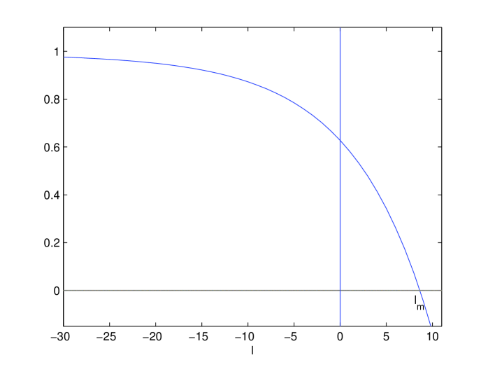
Figure 1: $b^{\prime}(r_{1})$ is plotted versus $l$.

Its main purpose is to give a qualitative picture of the allowed range on $l$.

According to Fig. 1, at $r=r_{1}$, $b^{\prime}(r_{1})<1$, so that $b(r_{1})<r_{1}$, and $b^{\prime}(r_{1})>0$ for all $l\leq l_{m}$ for some $l_{m}$ that depends on both $\alpha$ and $\omega$. For $l\leq 0$, we get a valid wormhole solution that includes both Lobo’s and Zaslavskii’s solutions. To understand the behavior for $l>0$, consider $b^{\prime}(\alpha r_{0})=0$ from Eq. (18). Solving for $\alpha$, we find that $l=l_{m}$ is implicitly determined by

$$\alpha=\left(\frac{l_{m}}{l_{m}+1}\frac{\omega}{\omega+1}\right)^{-\omega/(\omega+1+l_{m})},$$ (19)

which is well-defined since $\omega/(\omega+1)>0$. It should be noted that Fig. 1 is particularly helpful here because $l_{m}$ cannot be explicitly solved for. Moreover, the restriction $l\leq l_{m}$ is most severe at $r=r_{1}$, i.e., for any $r_{2}<r_{1}$, the above conditions on $b^{\prime}$ are automatically met on the interval $[r_{0},r_{1}]$, as can be seen from Fig. 2.

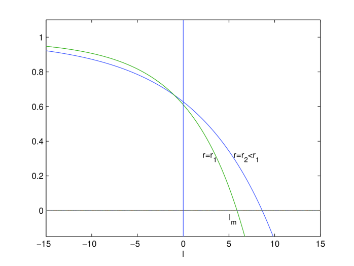
Figure 2: $b^{\prime}(r_{1})$ and $b^{\prime}(r_{2})$, $r_{1}<r_{2}$, plotted versus $l$.

5 Junction to an external vaccuum solution

As noted in the previous section, our wormhole spacetime is not asymptotically flat and must be cut off at some $r=r_{1}$ and joined to an exterior Scharzschild solution

$$ds^{2}=-\left(1-\frac{2M}{r}\right)dt^{2}+\frac{dr^{2}}{1-2M/r}+r^{2}(d\theta^{2}+\text{sin}^{2}\theta\,d\phi^{2}).$$ (20)

To facilitate the discussion, let us consider the cases $l\leq 0$ and $l>0$ separately,

5.1 $l\leq 0$

The junction at the cut-off requires continuity of the metric. As noted in Refs. [7, 8], the components $g_{\theta\theta}$ and $g_{\phi\phi}$ are already continuous due to the spherical symmetry. So we need to impose the continuity requirement only on the remaining components at $r=r_{1}$. These requirements imply that $\Phi_{\text{interior}}(r_{1})=\Phi_{\text{exterior}}(r_{1})$ and $b_{\text{interior}}(r_{1})=b_{\text{exterior}}(r_{1})$. In particular, we must have $2M=b(r_{1})$, where $b(r)$ is given in Eq. (13). Also

$$\left(\frac{r_{1}}{b_{0}}\right)^{l}=1-\frac{2M}{r_{1}},$$

whence

$$b_{0}=\frac{r_{1}}{(1-2M/r_{1})^{1/l}}.$$ (21)

While the metric is now continuous at the junction surface, the derivatives may not be. This needs to be taken into account when discussing the surface stresses; these are $\sigma$, the surface stress-energy, and $\mathcal{P}$, the surface pressure.

The following forms, proposed by Lobo [7, 8], are suitable for present purposes:

$$\sigma=-\frac{1}{4\pi r_{1}}\left(\sqrt{1-\frac{2M}{r_{1}}}-\sqrt{1-\frac{b(r_{1})}{r_{1}}}\right)$$ (22)

and

$$\mathcal{P}=\frac{1}{8\pi r_{1}}\left(\frac{1-\frac{M}{r_{1}}}{\sqrt{1-\frac{2M}{r_{1}}}}-[1+r_{1}\Phi^{\prime}(r_{1})]\sqrt{1-\frac{b(r_{1})}{r_{1}}}\right).$$ (23)

Since $b(r_{1})=2M$, the surface stress-energy $\sigma$ is zero. From $e^{2\Phi}=(r/b_{0})^{l}$, we find that $\phi^{\prime}(r)=l/(2r)$ and $r_{1}\Phi^{\prime}(r_{1})=l/2$. So Eq. (23) becomes

$$\mathcal{P}=\frac{1}{8\pi r_{1}}\left[\frac{1-\frac{M}{r_{1}}}{\sqrt{1-\frac{2M}{r_{1}}}}-\left(1+\frac{l}{2}\right)\sqrt{1-\frac{b(r_{1})}{r_{1}}}\right].$$

Letting $2M=b(r_{1})$ and simplifying, we get

$$\mathcal{P}=\frac{1}{8\pi r_{1}}\frac{-l+(1+l)\frac{b(r_{1})}{r_{1}}}{2\sqrt{1-\frac{b(r_{1})}{r_{1}}}}=\frac{1}{8\pi r_{1}}\frac{l\left(\frac{b(r_{1})}{r_{1}}-1\right)+\frac{b(r_{1})}{r_{1}}}{2\sqrt{1-\frac{b(r_{1})}{r_{1}}}}>0$$ (24)

since $l\leq 0$ and $b(r_{1})/r_{1}<1$. Also, from Eq. (4),

$$p_{r}(r_{1})=\frac{1}{8\pi r_{1}^{2}}\left[-\frac{b(r_{1})}{r_{1}}+\left(1-\frac{b(r_{1})}{r_{1}}\right)l\right],$$ (25)

it follows that $p_{r}(r_{1})$ is negative. Such a combination is to be expected since a negative radial pressure is needed to balance a positive surface pressure.

5.2 $l>0$

For positive $l$, our exact solution has a particularly interesting property: we can choose $r=r_{1}$ in such a way that the surface stresses are zero. Such a surface is called a boundary surface. To see how, we can use Eq. (13) to find

$$\frac{b(r_{1})}{r_{1}}=\frac{b(\alpha r_{0})}{\alpha r_{0}}=\frac{l}{\omega+1+l}+\frac{\omega+1}{\omega+1+l}\alpha^{-(\omega+1+l)/\omega}.$$ (26)

If $\alpha$ is chosen so that $b^{\prime}(\alpha r_{0})=0$ and $l=l_{m}$, then we get from Eq. (19),

$$\frac{b(r_{1})}{r_{1}}=\frac{l_{m}}{\omega+1+l_{m}}+\frac{\omega+1}{\omega+1+l_{m}}\left(\frac{l_{m}}{l_{m}+1}\frac{\omega}{\omega+1}\right)=\frac{l_{m}}{l_{m}+1}.$$ (27)

It now follows from Eq. (24) that $\mathcal{P}=0$. Since we already have $\sigma=0$, we conclude that for the case $l>0$, we can choose the cut-off $r=r_{1}$ in such a way that the junction surface is a boundary surface. We also note that from Eq. (25), $p_{r}(r_{1})=0$, as expected.

6 Galactic rotation curves

Returning to line element (7), if we use the form of $e^{2\Phi}$ in Eq. (9), we can recover line element (2), restated here for convenience:

$$ds^{2}=-\left(\frac{r}{b_{0}}\right)^{l}dt^{2}+e^{2\Lambda(r)}dr^{2}+r^{2}(d\theta^{2}+\text{sin}^{2}\theta\,d\phi^{2}).$$ (28)

To interpret this result, let us assume that $\omega>0$ in the equation $p=\omega\rho$. So we are no longer dealing with wormholes. Instead, the EoS has a cosmological interpretation as a perfect fluid but may also represent dark matter. This line element makes physical sense only if $l>0$ (even though our solution is mathematically correct for any $l$), since it is normally viewed as a model for galactic rotation curves. Here $l=2(v^{\phi})^{2}$, where $v^{\phi}$ is the tangential velocity and $b_{0}$ is an (arbitrary) integration constant [9, 10]. According to Ref. [11], $l=0.000001$ and remains approximately constant.

We conclude that line element (28) can be arrived at by purely mathematical means, i.e., given the Einstein field equations and the EoS $p=\omega\rho$, $\omega>0$, we get an exact solution only if $l$ in Eq. (9) is a constant. The implication is that a constant tangential velocity could have been hypothesized based on the Einstein field equations provided, of course, that a perfect-fluid background is assumed. The existence of a perfect fluid is a reasonable assumption that is also consistent with the existence of dark matter.

7 Conclusion

In this paper we obtained the most general possible exact solution of the Einstein field equations given a barotropic equation of state. This solution yields two different models. The condition $\omega<-1$ in the anisotropic EoS $p_{r}=\omega\rho$ yields the most general possible model for wormholes supported by phantom energy, thereby generalizing several earlier results. The case $\omega>0$ in the EoS $p=\omega\rho$ yields the usual model for galactic rotation curves. Here the EoS represents a perfect fluid which may include dark matter. Mathematicall speaking, we therefore have only one exact solution, but due to the parameter $\omega$, this solution corresponds to completely different physical models.

Acknowledgment: The author would like to thank Vance Gladney for many helpful discussions.

References

- [1] M.S. Morris and K.S. Thorne, “Wormholes in spacetime and their use for interstellar travel: A tool for teaching general relativity,” Amer. J. Phys. 56, 395-412 (1988).
- [2] F.S.N. Lobo, “Stable phantom energy traversable wormhole models,” arXiv: gr-qc/0603091.
- [3] S.V. Sushkov, “Wormholes supported by a phantom energy,” Phys. Rev. D 71, 043520 (2005).
- [4] P.K.F. Kuhfittig, “Seeking exactly solvable models of wormholes supported by phantom energy,” Class. Quant. Grav. 23, 5853-5860 (2006).
- [5] O.B. Zaslavskii, “Exactly solvable model of a wormhole supported by phantom energy,” Phys. Rev. D 72, 061303 (R) (2005).
- [6] S. Chandrasekhar, “A limiting case of relativistic equilibrium,” General Relativity, papers in honor of J. L. Synge, pp. 185-199 (1972).
- [7] F.S.N. Lobo, “Surface stresses on a thin shell surrounding a traversable wormhole,” Class. Quant. Grav. 21, 4811 (2004).
- [8] F.S.N. Lobo, “Phantom energy traversable wormholes,” Phys. Rev. D 71, 084011 (2005).
- [9] K.K. Nandi, I. Valitov, and N.G. Migranov, “Remarks on the spherical scalar field halo in galaxies,” Phys. Rev. D 80, 047301 (2009).
- [10] F. Rahaman, P.K.F. Kuhfittig, K. Chakraborty, K. Kalam, and D. Hossain, “Modeling galactic halos with predominantly quientessential matter,” Int. J. Theor. Phys. 50, 2655-2665 (2011).
- [11] K.K. Nandi, A.I. Filippov, F. Rahaman, S. Ray, A.A. Usmani, M. Kalam, and A. DeBenedictis, “Features of galactic halo in a brane world model and observational constraints,” Mon. Not. Roy. Astron. Soc. 399, 2079-2087 (2009).