An asymmetric jet launching model for the protoplanetary nebula CRL 618

Abstract

We propose an asymmetrical jet ejection mechanism in order to model the mirror symmetry observed in the lobe distribution of some protoplanetary nebulae (pPNe), such as the pPN CRL 618. 3D hydrodynamical simulations of a precessing jet launched from an orbiting source were carried out including an alternation in the ejections of the two outflow lobes, depending on which side of the precessing accretion disk is hit by the accretion column from a Roche lobe-filling binary companion. Both synthetic optical emission maps and position-velocity (PV) diagrams were obtained from the numerical results with the purpose of carrying out a direct comparison with observations. Depending on the observer’s point of view, multipolar morphologies are obtained which exhibit a mirror symmetry at large distances from the central source. The obtained lobe sizes and their spatial distribution are in good agreement with the observed morphology of the pPN CRL 618. We also obtain that the kinematic ages of the fingers are similar to those obtained in the observations.

1 Introduction

Explaining the multipolar morphology observed in proto planetary nebulae (pPNe) represents a challenge. Several mechanisms have been proposed in order to model the peculiar morphology exhibited by these objects.

Some of these mechanism are based on the hypothesis that the central source of the pPNe is actually a binary system. This idea was firstly invoked by Bond et al. (1978) (also Livio et al., 1979; Soker & Livio, 1994). The existence of a binary system inside of the pPN can produce collimated outflows when one of the components of the binary system, probably a white dwarf, accretes material from its companion, an AGB or post-AGB star (e.g. Morris, 1987; Soker & Rappaport, 2000). Subsequently, an accretion disk is formed and a bipolar jet or collimated fast wind (CFW) is ejected perpendicular to the plane of the disk (Frank & Blackman, 2004; Frank et al., 2007).

The pioneering 3D hydrodynamical simulations of Cliffe et al. (1995) showed that a precessing jet with a time-dependent ejection velocity can result in a point-symmetric nebula.

Following this idea, high-resolution 3D hydrodynamical simulations of a precessing jet with a time-dependent velocity were carried out in order to model the bipolar morphology of the pPNe Hen 3-1475 (Velázquez et al., 2004; Riera et al., 2004) and IC 4634 (Guerrero et al., 2008). Also, a precessing and continuous jet was used to reproduce both the morphology and emission of the PN K 3–35 (Velázquez et al., 2007) and the Red Rectangle (Velázquez et al., 2011).

Mirror and point-symmetric morphologies obtained from a precessing and continuous jet emanating from a binary system with circular orbits were studied by Raga et al. (2009). For orbital periods less than the precession period, these authors found that mirror symmetry is observed close to the central source, while point-symmetric morphologies prevail at larger distances (Masciadri & Raga, 2002; Raga et al., 2009). The influence of the orbital motion on the line emission of these objects was analyzed by Haro-Corzo et al. (2009). They found that the apparent mirror or point-symmetric morphology depends on the orientation of the object with respect to the observer.

The pPN CRL 618 exhibits a four-lobe mirror symmetric morphology. Numerical simulations have been carried out in the past with the intent of reproducing both the morphology and kinematics of this pPNe, such as the study of Lee & Sahai (2003) who proposed a scenario in which a CFW is interacting with a spherical AGB wind (see also Lee et al., 2009). Alternatively, Dennis et al. (2008) proposed that the multiple jet appearance of CRL 618 could be due to clumps moving outwards at high velocities and slightly different directions. Balick et al. (2013) have explored the nature of the jets of CRL 618 by means of 3D simulations of either a bullet or a continuous jet moving through the remnant AGB wind. These authors favour the ”bullet” hypothesis based on the multipolar morphology and the behaviour of the proper motion, which increases linearly with the distance from the central source. However, all these studies focus on modeling a single lobe.

By means of 3D hydrodynamical simulations, Velázquez et al. (2012) (see also Velázquez et al., 2013) have shown that the existence of a binary source where one of the stellar components (the primary star) ejects a spherical wind, while the orbiting companion (in elliptical orbit) emits a bipolar, precessing jet with time-dependent velocity, can generate multipolar geometries with results similar to the observed features in pPNe. These authors found that the large-scale morphological characteristics of these nebulae (lobe size, semi-aperture angle, number of observed lobes) can be related to some of the parameters of the binary system.

Soker & Mcley (2013) compare the morphologies of the pPN CRL618 and the young stellar object (YSO) NGC 1333 IRAS 4A2, and propose that their morphologies can be explained by means of “twin-jets”, e.g. two very narrow and nearby jets launched at the same time. They also consider that the origin of the jets is a binary system, with the components orbiting in very eccentric elliptical orbits. The “twin-jets” are emitted near periastron passages.

Recently, Riera et al. (2014) carried out an observational and numerical study of the pPN CRL 618. While the numerical model is based on the work of Velázquez et al. (2013), a time-decreasing trend was added to the jet velocity in the model description in order to guarantee consistency with the proper motion determined observationally by Riera et al. (2014). In spite of this, they obtain point-symmetric morphologies in their synthetic maps.

In this work, we have added a new ingredient to our description: an asymmetric jet ejection, i.e., we either let both the jet and counter-jet be launched simultaneusly, or we launch just one of them, depending on whether the accretion disk is close to being edge-on from the perspective of the companion star when the system pass through its periastron. This mechanism could explain the lobe distribution observed in the pPN CRL 618. This work is organized as follows: the assumptions of our model are given in section 2; the initial numerical setup is given in section 3; in section 4 we list our results; and finally in section 5 we summarize and discuss our results.

2 Model assumptions

Following the previous work of Raga et al. (2009); Velázquez et al. (2012, 2013) and Riera et al. (2014), we consider that a binary system is located at the centre of the pPN. One of the components of this binary system accretes material from the companion and launches a bipolar jet. The jet axis changes in time, forming a precession cone with a semi-aperture angle $\alpha$. The precession is retrograde with respect to the orbital motion (following the work of Terquem et al., 1999).

We assume that we have a jet with a periodic ejection velocity, with a period equal to the orbital period (Velázquez et al., 2012). Additionally, we impose a linear trend of decreasing ejection velocity with time in order to reproduce the observed behavior of the proper motion velocity (Riera et al., 2014).

In contrast to the scenario explored by Riera et al. (2014), in this work we consider an “asymmetrical jet ejection mechanism” which is inspired by the results of Montgomery (2012) and Fendt & Sheikhnezami (2013). The first of these papers presents a numerical study (by means of SPH simulations) of precessing acretion disks. Montgomery (2012) shows that because of the precession the accreting material falls only on one side of the accretion disk, producing asymmetries, or “humps”, in the density distribution. Fendt & Sheikhnezami (2013) studied how various disk perturbations can produce an asymmetrical jet ejection which can last for a few orbital periods. Several asymmetries have been reported in jets seen in YSOs. Hirth et al. (1994) performed a survey of T Tauri stars and found that about 50% of bipolar outflows observed in the optical exhibit differences between the velocities of the blueshifted and redshifted lobes that amount to factors of 1.5–2.5.

Recently, Matsakos et al. (2012) carried out both magnetohydrodynamic and resistive magnetohydrodynamics numerical simulations in order to explore intrinsic and extrinsic mechanisms which could explain the differences in the velocities observed in the blue and red components of YSO jets. The intrinsic mechanism is related to the configuration of the magnetic field of the central object, while the extrinsic one refers to the propagation of the jet into an inhomogeneous circumstellar medium (CSM). As an example of asymmetries due to the CSM we can mention the work of Podio et al (2011), which is based on observations of the DG Tauri B jets.

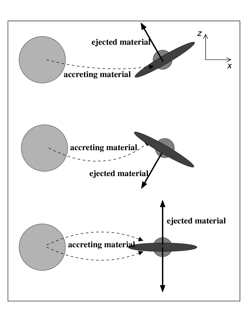
Figure 1: Schematic diagram of the ejection condition. The orbit lies on the $xy$–plane (the $y$-axis is perpendicular to the plane of the figure) and both foci of the elliptical orbit are on the $x$–axis.

The asymmetrical jet ejection mechanism proposed in this work is that the jet (or counter-jet) material is launched at periastron only when that side of the accretion disk is subject to an infall of accreted material, i.e., the jet (or counter-jet) is launched only when its axis is tilted towards the companion star when the stars are at periastron. When the accretion disk is nearly edge-on as seen from the companion star, both the jet and the counter-jet are launched. In practice, after running several tests we determined that the accretion disk can be considered edge-on when its axis is tilted with respect to the line joining the stars by angles larger than 87.5°(i.e., approaching an orbital configuration that is analogous to the Earth and Sun at solstice if the polar axis of the Earth is thought as the axis of the disk). A scheme of the assumed configuration is shown in Figure 1.

3 Initial setup of the numerical simulation

The 3D numerical simulations were performed with the Yguazú-a code (Raga et al., 2000). This code integrates the gasdynamical equations with a second order accurate scheme (in time and space) using the “flux-vector splitting” method of van Leer (1982) on a binary adaptive grid. Five levels of refinement were employed. Together with the gas-dynamic equations, several rate equations for atomic/ionic species were also integrated (for details about the species used, reaction equations, and cooling rates, see Raga et al., 2002).

The initial setup of the simulations is similar to that employed by Riera et al. (2014). The main differences are: (1) in the present work we impose an asymmetrical jet ejection, which was not studied in Riera et al. (2014); and (2) the jet is emitted at its maximum velocity when the system pass through periastron (see Eq.(1)).

At the center of a computational domain that spans (1.5, 1.5, 3)$\times 10^{17}$ cm (or $256\times 256\times 512$ cells at the highest resolution of the grid) along the $x$–, $y$– and $z$–axis, respectively, a bipolar jet is imposed as a cylinder of radius $r_{j}$ and length $l_{j}$, both equal to $3.6\times 10^{15}$ cm (equivalent to 6 pixels in the finest grid). The jet axis rotates on the surface of a precession cone with a half-opening angle $\alpha=15\arcdeg$. The precession period $\tau_{p}$ is four times the orbital period $\tau_{o}$, which has a value of 15.4 yr. The jet velocity is given by:

$$v_{j}=v_{j0}(t)\times\left[1+\Delta v\cos(\omega_{o}t)\right],$$ (1)

where $\Delta v=0.5$, $\omega_{o}=2\pi/\tau_{o}$, and $v_{j0}(t)$ is the mean jet velocity, which decreases linearly with time at a rate of $-3\ \mathrm{km\ s^{-1}\ yr^{-1}}$ and has a starting value of $400~{}\mathrm{km\ s^{-1}}$. The total number density of the jet was fixed at $10^{6}~{}\mathrm{cm^{-3}}$. With these values, the jet injects mass into the surrounding CSM at a rate $\dot{M}_{\mathrm{j}}=5.5\times 10^{-5}\mathrm{M_{\sun}\ yr^{-1}}$ ($6.6\times 10^{-3}\ \mathrm{M_{\sun}}$ are injected in 120 yr, the integration time of our simulations).

At $t=0$ yr, the jet axis projected on the $xy$-plane forms an angle of $-\pi/2$ with respect to the $x$–axis. Also, at this inital time, the whole computational domain is filled with a slow and dense AGB wind, with a density distribution given by Mellema (1995):

$$\rho(r,\theta)=\rho_{w}(r)\ f(\theta),$$ (2)

where $\rho_{w}(r)$ is given by (Mellema, 1995; Riera et al., 2014):

$$\rho_{w}=\frac{1}{2}\bigg{[}(\rho_{\mathrm{sup}}+\rho_{\mathrm{AGB}})+(\rho_{\mathrm{sup}}-\rho_{\mathrm{AGB}})\cos\epsilon\bigg{]}\bigg{(}\frac{r_{w}}{r}\bigg{)}^{2},$$ (3)

where

$$\epsilon=\pi\times\mathrm{min\bigg{[}1,\ max}\bigg{[}0,\ \frac{r-(r_{\mathrm{w}}+v_{\mathrm{w}}t_{\mathrm{sup}})}{v_{\mathrm{w}}t_{\mathrm{trans}}}\bigg{]}\bigg{]},$$ (4)

$r$ is the distance from the primary star, $v_{\mathrm{w}}$ is the terminal wind velocity, and $r_{\mathrm{w}}$ is the stellar wind radius. The times $t_{\mathrm{sup}}$ and $t_{\mathrm{AGB}}$ (see Eq. 3) indicate the duration of the superwind phase and the transition time between the AGB wind and the superwind phase, respectively; they were both chosen as 400 yr (Sánchez Contreras et al., 2002; Riera et al., 2014). The densities $\rho_{\mathrm{AGB}}$ and $\rho_{\mathrm{sup}}$ are calculated as:

$$\rho_{\mathrm{AGB/sup}}=\frac{\dot{M}_{\mathrm{AGB/sup}}}{4\pi\ r_{w}^{2}\ v_{w}}\,,$$ (5)

where $\dot{M}_{\mathrm{AGB}}$ and $\dot{M}_{\mathrm{sup}}$ are the mass loss rates of the AGB and the super phase AGB winds, respectively. We have chosen $\dot{M}_{\mathrm{AGB}}=10^{-5}{\mathrm{M_{\sun}\ yr^{-1}}}$, $\dot{M}_{\mathrm{sup}}=10^{-4}{\mathrm{M_{\sun}\ yr^{-1}}}$, $v_{w}=15\ {\mathrm{km\ s^{-1}}}$ (Sánchez Contreras et al., 2004; Nakashima et al., 2007; Bujarrabal et al., 2010; Lee et al., 2013), $r_{w}=3.6\times 10^{15}$ cm, and a constant temperature $T_{w}=100$ K.

Eq. (3)-(5) consider the mass-loss history of the AGB star (i.e. we have considered the final AGB stage, in which the star’s $\dot{M}$ increases). The function $f(\theta)$ (see Eq. 2) describes the angular dependence and can be written as

$$f(\theta)=1-\delta\frac{1-\exp(-2\beta\cos^{2}\theta)}{1-\exp(-2\beta)},$$ (6)

with $\theta$ being the angle with respecto to the $z$-axis. The parameters $\delta$ and $\beta$ where set to 0.7 and 5, respectively. Thus, the equator-to-pole density ratio is given by $1/(1-\delta)$. The parameter $\beta$ controls the shape of the density distribution. The value chosen here yields the density distribution of a flat and dense disk.

Furthermore, we have considered that the source of the jet describes an elliptical orbit around the barycenter of the system with an eccentricity of 0.5. Both foci of the orbit lie on the $x$–axis. Since the orbit itself is not resolved by the simulation, the effect of the orbital motion is to add a velocity component along the orbit to the jet velocity.

By using the temperature and density distributions obtained from the numerical simulations, we can compute the [S II]$\lambda\lambda 6716$,$6730$ emission coefficients. The intensities of these forbidden lines are calculated by solving five-level atom problems, using the parameters of Mendoza (1983). The [S II]$\lambda\lambda 6716$,$6730$ emission can be integrated along lines of sight to produce synthetic maps.

4 Results

We have carried out hydrodynamical simulations in which the asymmetrical jet ejection is either included (model M1) or not included (model M2). Model M2 is similar to that studied by Riera et al. (2014) for the case $\tau_{p}/\tau_{o}=4$. We let the hydrodynamical simulations of models M1 and M2 evolve until an integration time of $120$ yr. At this time, the lobes of the simulated pPN reach sizes similar to those observed in pPN CRL 618 if a distance of $1$ kpc is assumed (Riera et al., 2014).

4.1 Generating multipolar morphologies

Figure 2 shows the temporal evolution of the density stratification of model M1 by means of density cuts on the $xz$- and $yz$-planes (passing through the center of the computational domain). These sequences show the process through which a lobes distribution similar to that observed in the nebula CRL 618 can be reproduced. The flow velocity associated with the jet is displayed by white arrows; only velocities larger than 50 $\mathrm{km\ s^{-1}}$ are shown.

In all $yz$ density maps (bottom panels of Figure 2), a quadrupolar morphology is observed, exhibiting lobes with different sizes. Instead, the $xz$ density maps (upper panels of Figure 2) only show a bipolar lobe morphology. The formation of these structures can be understood by following the “launch sequence of the jet”, which is as follows: (1) at $t=0$ yr the top-left and the bottom-right lobes (hereafter lobes A and B, respectively) observed in the $yz$ density maps are launched; (2) at $t=\tau_{o}$ (as was previously mentioned, the jet velocity variability period is equal to the orbital period, $\tau_{o}$), the top-left lobe (hereafter lobe C) observed in the $xz$ density map is emitted; (3) at $t=2\tau_{o}$, both top-right and bottom-left lobes observed (hereafter lobes D and E) in the $xz$ density map are launched; (4) at $t=3\tau_{o}$ the bottom-left lobe (hereafter lobe F) observed in the $yz$ density map is ejected. This sequence is then repeated for subsequent times.

An interesting point to note is that the lobes A and B observed in the $yz$ density maps (see Figure 2) have different sizes despite being launched at the same time. This difference is caused by the orbital motion of the jet source and the density distribution around it. As the jet source passes trough periastron, the orbital speed reaches its maximum value of $\sim 30\mathrm{km\ s^{-1}}$. Although this value is small compared to the initial jet launching velocity (of $600~{}\mathrm{km\ s^{-1}}$), its vector addition is enough to cause a measurable difference in the directions of motion of the jets of $\sim 5\arcdeg$ (see the white arrows in Fig.2). Since the AGB wind material has the density distribution of a dense disk parallel to the $xy$ plane, the material of lobe B propagates in a denser medium than that of lobe A, thus decelerating quicker and causing lobe B to be shorter than lobe A. Similarly, the C lobe (shown in the $xz$ density maps) is the larger one because it propagates into the cavity created by the previous lobes, which has a lower density.

4.2 Synthetic maps: comparison with observations

With this launching sequence of the jet, we expect to obtain morphologies similar to that of CRL 618 if we “observe” the system along the $y$ direction, i.e., when the line of sight is aligned with the $y$ axis. In order to test this, synthetic [S II] emission maps (shown in Figure 3) were obtained from the numerical results of models M1 and M2 considering different lines of sight. These maps were generated considering that the precession axis lies on the plane of the sky ($\phi=0\arcdeg$). The top panels of Figure 3 show the $xz$ and $yz$ projections (left and right panels, respectively) for model M1, while the bottom panels show the corresponding map projections for model M2. The main differences between these models are evident by comparing the morphology of the two maps obtained for the $xz$ projection. On the one hand, the morphology obtained for model M2 shows six lobes, while four lobes are observed for model M1. On the other hand a clear point-symmetric lobe distribution is observed in the map of the model M2, while the map for model M1 displays an almost mirror-symmetric “nebula”, which resembles the observed morphology of the pPN CRL 618. The size and orientation of the upper lobes of the synthetic nebula are similar to the observed Eastern lobes of the pPN CRL 618. A similar agreement is observed for the bottom lobes. In addition, the $xz$ projection map of model M1 (see Figure 3) reveals a remarkable difference in the morphology and the size of the lobes corresponding to the jet and the counter-jet.

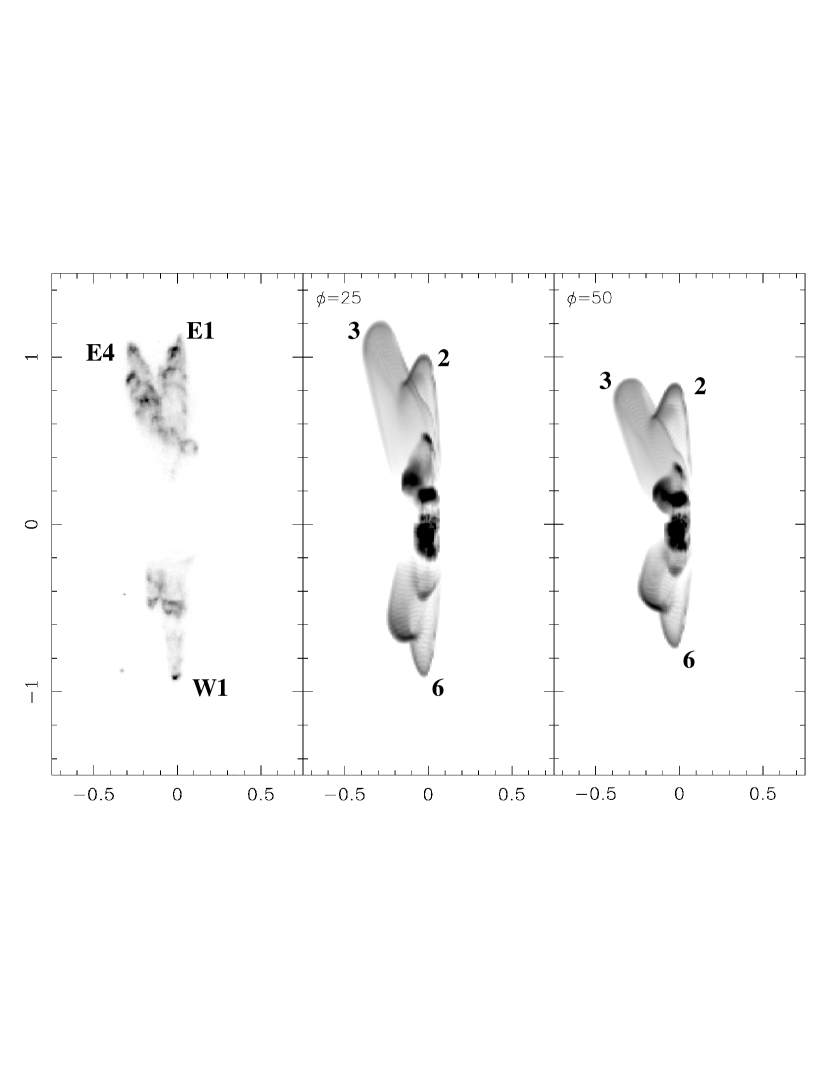
Figure 4: Direct comparison between the observed (left panel) and synthetic [S II] images (middle and right panels). The synthetic [S II] maps ($xz$ projection) were obtained considering that the precession axis is tilted by either 25°or 50°(middle and right panels, respectively) with respect of the plane of the sky. The horizontal and vertical axes are given in units of $10^{17}$ cm. The three more evolved fingers have been labeled in order to facilitate the comparison (as described in the text).

A direct comparison between observations and synthetic emission maps is shown in Figure 4. The observed [S II] image of the pPN CRL 618 is displayed on the left, while the middle and the right panels show the $xz$ projection of the synthetic emission map considering angles between the precession cone axis and the plane of the sky of 25°(middle) and 50°(right). The orientation of the observed nebula with respect to the plane of the sky is not precisely determined, with estimates ranging from 20°to 40°(Sánchez-Contreras et al. 2002). In order to facilitate the comparison we have labeled three fingers in the observed image as E1, E4 and W1, following the labeling given by Balick et al. (2013). Also, on the synthetic maps, several “bow shock” features were labeled with numbers from 1 to 6. Synthetic maps reveal a four-fingered structure. In order to identify these fingers, we employ the number of the bow shock features located at the finger tip. Finger “2” is the overlap, along the line of sight, of the lobes labeled as “A” and “E”, which were mentioned in the previous subsection, while finger “6” is the overlap of lobes “B” and “E”. Fingers “3” and “5” correspond to lobes “C” and “F”, respectively. It must be noted that while the overall size of the “synthetic nebula” for the 25°case (middle panel of Figure 4) is similar to the observed one (if a distance of 1 kpc is considered), the sizes of fingers “2” and “3” are dissimilar, in contrast to the observations. The size of fingers “2” and “3” becomes similar if the angle is 50°(right panel). However, in this case, the “synthetic nebula” is somewhat smaller than the observed one for the same assumed distance.

4.3 Proper motions and PV diagram

Employing the synthetic maps, we carried out a proper motion study. As in Riera et al. (2014), the simulations were restarted from the output obtained at an integration time of 120 yr and they were left to evolve 10 yr longer. The two ouputs are then compared to one another. The results obtained from this proper motion study are shown in Figure 5 and summarized in Table 1. The main resul is that the kinematic ages of fingers “2”, “3”, and “6” found by this analysis turn out to be very similar to each other ($\sim 100$ yr) for both orientations with respect to the plane of the sky that we have considered. This is in good agreement with the kinematic ages obtained by Balick et al. (2013) for fingertips E1, E4, and W1, determined by using both F606W and F656N images of the pPN CRL 618.

This result could look like striking because actually finger “3” was ejected 15 yr after the launching of fingers “2” and “6” (see subsection 4.1). This is, we would expect that the finger 3 turns out to be 15 yr younger than fingers “2” and “6”. However it is necessary to take into account that the material associated to fingers “2” and “6” do not follow a ballistic trajectory because at the beginning they move into a dense CSM. Instead, the gas of finger “3”, which was launched later, propagates into the lower density cavity which was previously excavated by the material belonging to fingers “2” and “6” (or lobes “A” and “B”, see subsection 4.1), thus evolving faster.

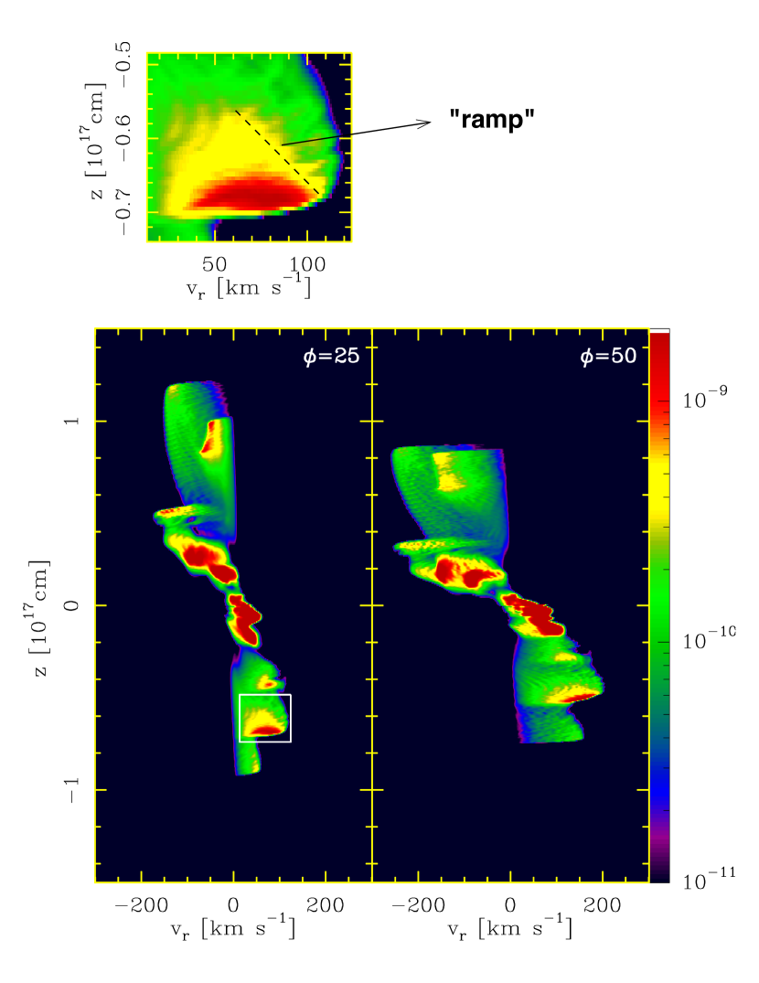
Figure 6: PV diagrams obtained for model M1 ($xz$ projection) considering angles between the precession axis of the jet and the plane of the sky of 25°(left panel) and 50°(right panel). The vertical logarithmic color scale gives de flux in units $\mathrm{erg\ s^{-1}\ cm^{-2}\ sr^{-1}}$. The upper panel is an enlargement of the rectangular white region in the left panel.

Figure 6 displays PV diagrams (bottom panels) for model M1 ($xz$ projection) considering both orientations with respect to the plane of the sky. As in the Figure 3 of Riera et al. (2011), the PV diagrams display several ramps in radial velocity. This is clearly shown in the enlargement (upper panel) of the white rectangular region in the left panel. Furthermore, the jet ejection mechanism employed in this work produces clear differences in both the emission and the radial velocities of the blue- and the red-shifted components. The radial velocities differ by factors which lie in the range 1.3–2, which is consistent with the values reported by Hirth et al. (1994).

5 Discussion and conclusions

As was mentioned above, it is not uncommon to find asymmetries in the jet velocities of HH objects, with factors between the blue and red components of about 1.5–2.5 (Hirth et al., 1994). The nature of these asymmetries can be intrinsic, which is related to the ejection mechanism itself, or extrinsic, where the properties of the CSM determine the shapes and sizes of lobes and their expansion velocities (Matsakos et al., 2012). It can be expected that the asymmetries observed in jets of pPNe share the same nature as those seen in the jets of HH objects.

Recently, Steffen et al. (2013) reproduced multipolar morphologies by means of the interaction of a fast isotropic wind with a very inhomogeneous CSM, an idea that can be classified under the extrinsic origin possibility.

In contrast to this, the “twin-jets” mechanism proposed by Soker & Mcley (2013) belongs to the intrinsic class. This mechanism is based on the existence of a binary system at the center of the object, and it consists in that two narrow jets are emitted at the same time from a narrow region when the jet source passes through periastron. With this scenario, they explain the morphology observed in the pPN CRL618 and in the YSO NGC 1333 IRAS 4A2.

The asymmetric jet ejection mechanism that we propose in this work also belongs to the intrinsic origin hypothesis. We study the effects of an imposed alternation (between the two outflow lobes) of the ejection on the nebular morphology. Depending on the orientation of the system with respect to the observer, large scale morphologies with a mirror symmetry are obtained, such as that observed in the pPN CRL 618. The main observational kinematic features such as PV diagrams (Riera et al., 2011) and proper motions (Riera et al., 2014) are recovered. Also, the PV diagram corresponding to model M1 shows differences in the radial velocities between the blue and the red components by factors of 1.3–2, which is in agreement with the result of Hirth et al. (1994), for the case of HH objects. Furthermore, the kinematic ages of the fingers obtained from our numerical study are in a very good agreement with those reported by Balick et al. (2013).

As we have pointed out in the past (Masciadri & Raga, 2002; Raga et al., 2009), an orbital motion of the jet source can result in mirror symmetries of the outflow lobes. However, the relatively low orbital velocities possible for the sources of observed mirror-symmetric pPNe cannot be responsible for the large angular deviations of their outflow lobes (Velázquez et al., 2013; Riera et al., 2014).

In the simulations presented above, we show that a jet ejection episodes that alternate between the two sides of the accretion disk (synchronized with the precession of the disk) can indeed produce the observed mirror-symmetric multi-lobe structures. This presents a very interesting alternative to the “twin-jet” model for explaining the mirror-symmetric lobes with large angular deviations observed in some PPNe.

Figure 2: Density stratification maps obtained at integration times of 60, 90, and 120 yr. The upper (bottom) panels display the $xz$ ($yz$) cut of the density stratification, passing through of the computational domain center, where the vertical axis corresponds to the $z$ direction. The white arrows show the velocity field of the flow. The horizontal arrow at the bottom left of the bottom right panel indicates a velocity of $200~{}\mathrm{km\ s^{-1}}$. The horizontal bar is the logarithmic color-scale of the density, which is given in units of $\mathrm{g\ cm^{-3}}$. Both axes are displayed in units of $10^{17}$ cm. In order to facilitate the description of the density evolution, the lobes observed in both $yz$ and $xz$ projections (right panels) were labeled with capital letters from A to F (see text).

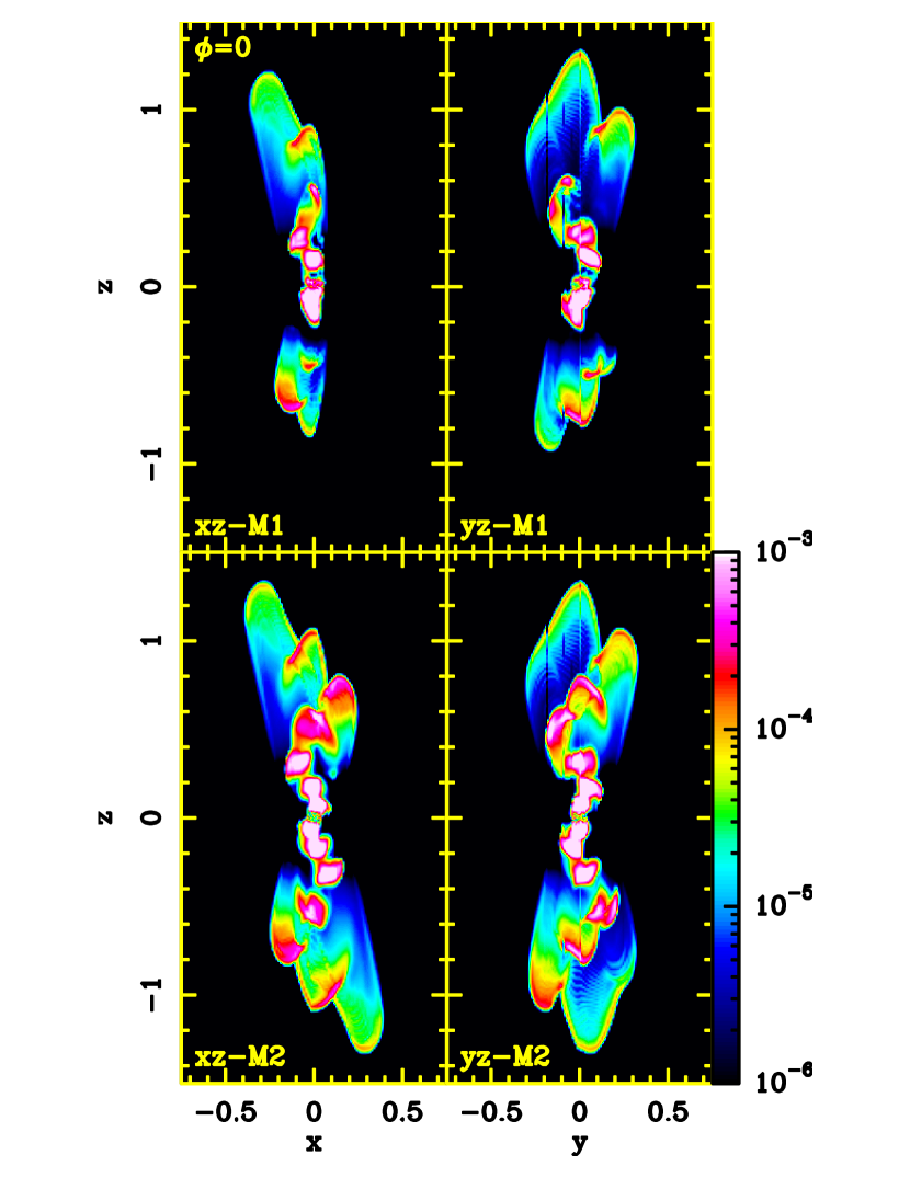
Figure 3: Synthetic [S II] emission maps obtained from the numerical simulations. The upper panels display the $xz$ (left) and $yz$ (right) projections for the model M1. The $z$–axis of the computational domain lies on the plane of the sky ($\phi=0$). The bottom panels display the same but for model M2. Both axes are given in units of $10^{17}$ cm. The vertical color bar indicates the [S II] emission in units of $\mathrm{erg\ s^{-1}\ cm^{-2}\ sr^{-1}}$.

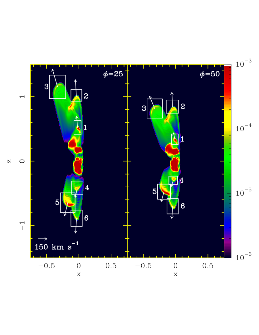
Figure 5: Proper motions of the individual features (labeled from 1 to 6) obtained for the [S II] synthetic maps (model M1) at $\phi=25$°(left panel) and $\phi=50$°(right panel). The white boxes show the regions that were used to perform the proper motion study. The arrows indicate the velocities of the features in the plane of the sky (see Table 1). The horizontal white arrow at the bottom left of the left panel indicates a proper motion of $150~{}\mathrm{km\ s^{-1}}$. The logarithmic color scale gives the [S II] flux in units of $\mathrm{erg\ s^{-1}\ cm^{-2}\ sr^{-1}}$.

Table 1: Proper motion velocities corresponding to Figure 5

Feature	$\phi$	Distance	$v_{x}$	$v_{z}$	$v_{t}$	kinematic age
	[°]	[$10^{17}$ cm]	[$\mathrm{km\ s^{-1}}$]	[$\mathrm{km\ s^{-1}}$]	[$\mathrm{km\ s^{-1}}$]	[yr]
1	25.0	0.50	-15.0	210.0	211.0	79.0
1	50.0	0.34	-24.0	122.0	124.0	87.0
2	25.0	1.00	-18.0	303.0	304.0	108.0
2	50.0	0.85	-8.9	262.0	262.0	102.0
3	25.0	1.20	-93.0	322.0	335.0	114.0
3	50.0	0.88	-95.0	228.0	247.0	113.0
4	25.0	0.40	-39.0	-178.0	182.0	72.0
4	50.0	0.30	-34.0	-113.0	118.0	81.0
5	25.0	0.70	-55.8	-246.0	252.0	84.0
5	50.0	0.51	-50.0	-181.0	188.0	86.0
6	25.0	0.90	-18.0	-266.0	267.0	106.0
6	50.0	0.70	-14.0	-221.0	222.0	100.0

References

- Balick et al. (2013) Balick, B., Huarte-Espinosa, M., Frank, A., et al. 2013, ApJ, 772, 20
- Bond et al. (1978) Bond, H. E., Liller, W., & Mannery, E. J. 1978, ApJ, 223, 252
- Bujarrabal et al. (2010) Bujarrabal, V., Alcolea, J., Soria-Ruiz, R., et al. 2010, A&A, 521, L3
- Cliffe et al. (1995) Cliffe, J. A., Frank, A., Livio, M., & Jones, T. W. 1995, ApJ, 447, L49
- Dennis et al. (2008) Dennis, T.J., Cunningham, A.J., Frank, A., Balick, B., Blackman, E.G. & Mitran, S. 2008, ApJ, 679, 1327
- Frank & Blackman (2004) Frank, A., & Blackman, E. G. 2004, ApJ, 614, 737
- Frank et al. (2007) Frank, A., De Marco, O., Blackman, E., & Balick, B. 2007, arXiv:0712.2004
- Fendt & Sheikhnezami (2013) Fendt, C., & Sheikhnezami, S. 2013, ApJ, 774, 12
- Guerrero et al. (2008) Guerrero, M. A., et al. 2008, ApJ, 683, 272
- Haro-Corzo et al. (2009) Haro-Corzo, S. A. R., Velázquez, P. F., Raga, A. C., Riera, A., & Kajdic, P. 2009, ApJ, 703, L18
- Hirth et al. (1994) Hirth, G. A., Mundt, R., Solf, J., & Ray, T. P. 1994, ApJ, 427, L99
- Lee & Sahai (2003) Lee, C.-F., & Sahai, R. 2003, ApJ, 586, 319
- Lee et al. (2009) Lee, C.-F., Hsu, M.-C. & Sahai, R. 2009, ApJ, 696, 1630
- Lee et al. (2013) Lee, C.-F., Sahai, R., Sánchez Contreras, C., Huang, P.-S., & Hao Tay, J. J. 2013, ApJ, 777, 37
- Livio et al. (1979) Livio, M., Salzman, J., & Shaviv, G. 1979, MNRAS, 188, 1
- Masciadri & Raga (2002) Masciadri, E., & Raga, A. C. 2002, ApJ, 568, 733
- Matsakos et al. (2012) Matsakos, T., Vlahakis, N., Tsinganos, K., et al. 2012, A&A, 545, A53
- Mellema (1995) Mellema, G. 1995, MNRAS, 277, 173
- Montgomery (2012) Montgomery, M. M. 2012, ApJ, 745, L25
- Morris (1987) Morris, M. 1987, PASP, 99, 1115
- Nakashima et al. (2007) Nakashima, J.-i., Fong, D., Hasegawa, T., et al. 2007, AJ, 134, 2035
- Podio et al (2011) Podio, L., Eislöffel, J., Melnikov, S., Hodapp, K. W., & Bacciotti, F. 2011, A&A, 527, A13.
- Raga et al. (2000) Raga, A. C., Navarro-González, R., & Villagrán-Muniz, M. 2000, Rev. Mexicana Astron. Astrofis., 36, 67
- Raga et al. (2002) Raga, A. C., de Gouveia Dal Pino, E. M., Noriega-Crespo, A., Mininni, P. D., & Velázquez, P. F. 2002, A&A, 392, 267
- Raga et al. (2009) Raga, A. C., Esquivel, A., Velázquez, P. F., Cantó, J., Haro-Corzo, S., Riera, A., & Rodríguez-González, A. 2009, ApJ, 707, L6
- Riera et al. (2004) Riera, A., Velázquez, P. F., & Raga, A. C. 2004, Asymmetrical Planetary Nebulae III: Winds, Structure and the Thunderbird, 313, 487
- Riera et al. (2011) Riera, A., Raga, A. C., Velázquez, P. F., Haro-Corzo, S. A. R., & Kajdic, P. 2011, A&A, 533, A118
- Riera et al. (2014) Riera, A., Velázquez, P. F., Raga, A. C., Estalella, R., & Castrillón, A. 2014, A&A, 561, A145
- Sánchez Contreras et al. (2002) Sánchez Contreras, C., Sahai, R., & Gil de Paz, A. 2002, ApJ, 578, 269
- Sánchez Contreras et al. (2004) Sánchez Contreras, C., Bujarrabal, V., Castro-Carrizo, A., Alcolea, J., & Sargent, A. 2004, ApJ, 617, 1142
- Steffen et al. (2013) Steffen, W., Koning, N., Esquivel, A., et al. 2013, MNRAS, 436, 470
- Soker & Livio (1994) Soker, N., & Livio, M. 1994, ApJ, 421, 219
- Soker & Rappaport (2000) Soker, N., & Rappaport, S. 2000, ApJ, 538, 241
- Soker & Mcley (2013) Soker, N., & Mcley, L. 2013, ApJ, 772, L22
- Terquem et al. (1999) Terquem, C., Eislöffel, J., Papaloizou, J. C. B., & Nelson, R. P. 1999, ApJ, 512, L131
- van Leer (1982) van Leer, B. 1982, in Lecture Notes in Physics, Vol. 170, Numerical Methods in Fluid Dynamics, ed. E. Krause (Berlin:Springer)
- Velázquez et al. (2004) Velázquez, P. F., Riera, A., & Raga, A. C. 2004, A&A, 419, 991
- Velázquez et al. (2007) Velázquez, P. F., Gómez, Y., Esquivel, A., & Raga, A. C. 2007, MNRAS, 382, 1965
- Velázquez et al. (2011) Velázquez, P. F., Steffen, W., Raga, A. C., Haro-Corzo, S., Esquivel, A., Cantó, J., & Riera, A. 2011, ApJ, 734, 57
- Velázquez et al. (2012) Velázquez, P. F., Raga, A. C., Riera, A., Steffen, W., Esquivel, A., Cantó, J., & Haro-Corzo, S. 2012, MNRAS, 419, 3529
- Velázquez et al. (2013) Velázquez, P. F., Raga, A. C., Cantó, J., Schneiter, E. M., & Riera, A. 2013, MNRAS, 428, 1587