Analytical solution of electronic transport through a benzene molecule using lattice Green’s functions

Abstract

Using a Green’s function formalism we derive analytical expressions for the electronic transmittance through a benzene ring. To motivate the approach we first solve the resonant level system and then extend the method to the benzene case. These results can be used to validate numerical methods.

1 Introduction

The transport through molecules as small as benzene [1] or as long as DNA [2] or carbon nanotubes [3] falls into the realm of molecular electronics. This field of research has a long history [4], dating back to 1956 [5]. As a consequence of this latter paper and of the immediate perception of its importance the USA Air Force decided, already by that time, to fund this type of research [6].

According to Cuevas and Scheer [6] molecular electronics is the field of research devoted to the study of the electronic and thermal transport through individual molecules. The objective of this type of research is to produce electronic devices where the building blocks are single molecules, exploring the quantum mechanical properties that necessarily appear at this small length scales. This type of devices include: switches, sensors, diodes, transistors, and other [7]. On the other hand, another advantage of this approach is that it opens the door to the discovery of new quantum phenomena. In this sense, one should remember that, historically, technological breakthroughs were often a natural consequence of the explorations of new areas, and not its finality. From a technological point of view, there are several advantages in pursuing the study of molecular electronics when compared to the present silicon technology, namely [6, 8]:

• Size. Molecules have typical sizes ranging from $1$ to $100$ nm, which allows the construction of functional nano-structures with subsequent advantages in cost, efficiency and power dissipation.

• Speed. Estimations show that a good molecular wire could, for example, reduce the transit time of a traditional transistor, around $10^{-14}$ s, hence obtaining faster operations.

• New functionalities. As an example, many molecules have several stable geometric structures, or isomers, that may have different electronic or optic properties, what can be an advantage for the development of some devices, such as switches or sensors.

• Synthetic tailorability. By changing, for example, the composition or the geometry of a system, one can obtain specific transport or optical properties suitable for a specific end.

However, we need not only to know which molecules are the best for a certain usage, but also how to connect them, namely through unidimensional (1D) nanowires. We shall focus now on the composition of these nanowires, rather than on how to create them (for that, see, for example [[6]]).

Historically, the carbon-based molecules always played an important role in the field of molecular electronics, due to its high versatility. Carbon is the basis of a wide range of structures, since tridimensional, like diamonds or graphite, to bidimensional, like graphene, (quasi)unidimensional, like the nanotubes, or even (quasi)zero-dimensional, like the fullerenes. In particular, the carbon nanotubes can be used to connect individual molecules. Also, some experiments on quantum transport through carbon nanotubes have already been performed [9].

Another very important class of systems, related to the previous one, are the hydrocarbons. The importance of this class is that such molecules can have different transport properties depending on the degree of hybridization of the molecular orbitals of its carbon atoms. If the valence electrons are $sp^{3}$ hybridized, there is a tetrahedral arrangement of the bonds in space. This is the case of the alkanes, with the sum formula $C_{n}H_{2n+2}$ [the simplest alkane, the ethane, is presented in figure 1(a)]. Since each valence electron is used for the formation a different (single) chemical bond, they are basically localized, and thus the alkanes are insulating. On the other hand, the valence electrons may also be $sp^{2}$ or $sp$ hybridized, forming, respectively, alkenes, with double bonds, and alkynes, with triple bonds [the simplest of each kind, the ethylene and the acethylene, are presented in figure 1(b) and (c)]. A particular case of these occurs when double or triple bonds are alternated with single bonds. These molecules are very stable and give rise to delocalized wave functions, which makes them good conductors.

(a) Ethane.

(b) Ethylene.

(c) Acetylene.

Figure 1: This figure shows schematic representations of the simplest of each type of hydrocarbon: (a) the ethane, (b) the ethylene and (c) the acetylene. These are, respectively, an alkane, an alkene and an alkyne.

Another advantage of these organic molecules is that they can assume different geometries. For example, in figure 2 are presented two polyenes with six carbon atoms each. Due to their atoms’ $sp^{2}$ hybridization, they tend to make 120^o angles between bonds. When the angles are built to alternate sides, the polyene has a zigzag shape [hexatriene, figure 2(a)]. However, when all angles are built to the same side, the polyene has a cyclic shape [benzene, figure 2(b)]. In the particular case of the benzene, there is a fully delocalized double bond, which makes this molecule a good conductor. This is the motivation of our study of the transport through a benzene ring.

(a) Hexatriene.

(b) Benzene.

Figure 2: This figure shows the schematic representation of two different molecules with six carbon atoms each: (a) a hexatriene, with zigzag structure, and (b) a benzene, with a cyclic structure. The dashed lines on the benzene indicate fully delocalized double bonds.

The main goal of this paper is to provide a theoretical introduction to molecular electronics, studying the electronic transport through a benzene ring, using the formalism of Green’s functions. The transport through quantum rings has been considered in the literature before [10], but the approach used cannot be easily generalized to more complex problems. On the other hand, the Green’s function approach is the method of choice when the complexity of the problem increases. The use of the Green’s function method to describe impurity states in a tight-binding models has also been considered [11]. The effect of phonons on transport across a Benzene molecule has also been considered using Green’s function methods [12].

The paper is written with the graduate students in mind. The method of Green’s function is often considered a difficult one, casting a way many students from its study. Here we show, by two examples of moderate complexity, that this is not the case. These two problems are solved analytically, which, to our best knowledge has not been solved in the literature before using the given method. Indeed, although, there are many books on quantum transport, none give a detailed discussion of problems of moderate complexity. Typically, they solve the one-dimension tight-binding model [13, 14]. The same happens with review articles [15]. We thus consider that the solution of this problem is a valuable addition to the literature.

2 Formalism and the resonant level system

The resonant level system is the simplest example of molecular electronics displaying non-trivial transport properties (this model also describes the transport through a single quantum level [16]). We introduce the formalism used in the next section for describing electronic transport through a benzene molecule with a hands-on philosophy by solving the resonant level system using Green’s functions. This approach will benefit the students wanting to have a working knowledge of the method.

To explain the basics of the Green’s functions formalism, let us consider a problem that can be described by a Hamiltonian written in the form

$$H=H_{0}+V,$$ (1)

such that

$$H_{0}\left|\psi_{0}\right>=E\left|\psi_{0}\right>$$ (2)

and

$$H\left|\psi\right>=E\left|\psi\right>.$$ (3)

Let us also consider that $\left|\psi_{0}\right>$ and $\left|\psi\right>$ are such that they can be related by

$$\left|\psi\right>=\left|\psi_{0}\right>+\left|\psi_{S}\right>,$$ (4)

where $\left|\psi_{S}\right>$ represents the scattered component of the wave. From the previous equations, one can easily find the Lippmann-Schwinger equation, of the form

$$\left|\psi\right>=\left|\psi_{0}\right>+G_{0}\cdot V\left|\psi\right>,$$ (5)

where we define the free Green’s function operator as [17]

$$G_{0}\equiv\frac{1}{E-H_{0}+i\epsilon}.$$ (6)

This definition is obtained naturally except for the term $i\epsilon$, where $\epsilon$ is a infinitesimal positive real number. This term is added to the definition to guarantee that this operator describes a wave propagating from the left to the right.

Furthermore, one can replace the term $\left|\psi\right>$ on right hand side of the Lippmann-Schwinger equation (5) with itself obtaining by iteration

$$\left|\psi\right>=\left|\psi_{0}\right>+G\cdot V\left|\psi_{0}\right>,$$ (7)

where $G$ is the full Green’s function operator, that can be defined as

$$G\equiv\frac{1}{1-G_{0}\cdot V}\cdot G_{0}.$$ (8)

The advantage of Eq. (7) is that only the known wave function $\left|\psi_{0}\right>$ enters in it. Recalling the explicit definition of $G_{0}$, given in (6), the previous equation can be simplified to

$$G\equiv\frac{1}{E-H_{0}-V+i\epsilon},$$ (9)

which results in a definition analogue to that of $G_{0}$ except that now the full Hamiltonian enters in the definition, and with $\epsilon$ having the same meaning as before. However, neither of the two previous definitions of $G$ are very useful, since both of them involve inversions of operators, which can be difficult. Fortunately, the Green’s function operator can yet be written in a third form, through a Taylor expansion of the term $\left(1-G_{0}\cdot V\right)^{-1}$ in (8). In doing so, one reaches Dyson’s equation

$$G=G_{0}+G_{0}\cdot V\cdot G.$$ (10)

Its usefulness will be proven further in the text.

The key aspect of this method is to use the previous relations in order to obtain, in the end, an expression of the form

$$\left<n\middle|\psi\right>= C\left(e^{ikan}+re^{-ikan}\right), n<0$$ , (11)

$$\left<n\middle|\psi\right>= C\left(\tau e^{ikan}\right), n>0$$ . (12)

where $C$ is some constant and $\left|n\right>$ is a position state (we note that we have in mind a description of our systems by tight-binding Hamiltonians; therefore $\left|n\right>$ is a Wannier state). From an expression of this form, it is possible to obtain $r$ and $\tau$, which are respectively the reflection and transmission amplitudes, such that the reflectance and transmittance through some defect, quantum dot, or molecule are given by

$${\cal R}=\left|r\right|^{2}$$ (13)

and

$${\cal T}=\left|\tau\right|^{2}.$$ (14)

We now proceed to the study of the resonant level system. This problem will be useful to illustrate the previously described method in a situation where the solution is non-trivial (in general, textbooks tend to describe only trivial examples which produce some discomfort on the students). To start with, let us define the system we ought to study. This is composed of two semi-finite 1D chains, with $N$ atoms each, and a different atom in between them – which we shall call the defect. The distance between each atom and its nearest two neighbours is $a$. In both 1D chains, the hopping energy between two first neighbours is $-t$, whereas the hopping energy between higher order neighbours is zero. However, due to the presence of the defect, we shall consider that, on the one hand, the hopping energies around the defect are different from $-t$ and are different in both sides of it – being $-\alpha_{\mathrm{L}}$ to the left and $-\alpha_{\mathrm{R}}$ to the right –, and, on the other hand, there is an on-site energy on the position of the defect ($n=0$), with value $-\varepsilon_{0}$. In figure 3 there is a schematic representation of the described system.

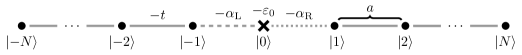
Figure 3: Schematic representation of the one level resonant system considered. This system is composed of two 1D chains with $N$ atoms each, represented by circles, and a defect in the middle of them, represented by a cross. In this figure are also identified the hopping energies between different atoms ($-t$, $-\alpha_{\mathrm{L}}$ or $-\alpha_{\mathrm{R}}$, accordingly), the site energy on the defect ($-\varepsilon_{0}$) and the distance between two neighbours ($a$).

From the previous description, it becomes clear that the Hamiltonian which describes this system can be written as

$$H=H_{\mathrm{L}}+H_{\mathrm{R}}+H_{\mathrm{C}}+V\equiv H_{0}+V,$$ (15)

where we shall define

$$H_{\mathrm{L}}=-t\sum_{n=-N}^{-2}\Big{(}\left|n\right>\left<n+1\right|+\left|n+1\right>\left<n\right|\Big{)},$$ (16)

$$H_{\mathrm{C}}=-\varepsilon_{0}\left|0\right>\left<0\right|,$$ (17)

$$H_{\mathrm{R}}=-t\sum_{n=1}^{N-1}\Big{(}\left|n\right>\left<n+1\right|+\left|n+1\right>\left<n\right|\Big{)}$$ (18)

and

$$V=-\alpha_{\mathrm{L}}\Big{(}\left|-1\right>\left<0\right|+\left|0\right>\left<-1\right|\Big{)}-\alpha_{\mathrm{R}}\Big{(}\left|0\right>\left<1\right|+\left|1\right>\left<0\right|\Big{)}.$$ (19)

We assume that in the beginning of times (say $t=-\infty$) the two semi-infinite chains (often called leads in molecular electronics terminology) are decoupled from the central atom. In this case a flux of electrons incoming from the left of the defect ($n<0$) cannot continue to the $n=0$ position being reflected in the end of the semi-infinite lead. This means that at $t=-\infty$ the unperturbed wave function must read

$$\left|\psi_{0}\right>= \left|\psi_{\mathrm{L}}\right>, n<0$$ , (20)

$$\left|\psi_{0}\right>= 0, n>0$$ , (21)

where $\left|\psi_{\mathrm{L}}\right>$ is such that

$$H_{\mathrm{L}}\left|\psi_{\mathrm{L}}\right>=E\left|\psi_{\mathrm{L}}\right>,$$ (22)

where $\left|\psi_{\mathrm{L}}\right>$ plays the role of $\left|\psi_{0}\right>$ in the formalism described above. Hence, to apply the previously described method, we must find $\left|\psi_{\mathrm{L}}\right>$. It can be written, in general, in a basis composed by every position state available, that is,

$$\left|\psi_{\mathrm{L}}\right>=\sum_{m=-N}^{-1}c(m)\left|m\right>,$$ (23)

where we do not know yet the explicit form of the coefficients $c(m)$. However, we can use this result, as well as the definition of $H_{\mathrm{L}}$ given in (16), and replace them in (22). Multiplying both sides of the resulting equation with the position state $\left<l\right|$ ($l=-N,\ldots,-1$), one gets that (called the tight-binding equations)

$$-tc(-N+1)=Ec(-N), l=-N$$ , (24)

$$-t\left[c(l+1)+c(l-1)\right]=Ec(l), -N<l<-1$$ , (25)

$$-tc(-2)=Ec(-1), l=-1$$ . (26)

It should be clear that (25) becomes general if we introduce the condition

$$c(-N-1)=c(0)=0,$$ (27)

where it is assumed that $N$ will tend to infinite in the of the calculation. On the other hand, we can consider that the flux must be composed by the sum of two plane waves, one travelling forward and the other travelling backward, which means that the coefficients $c(m)$ must have the form

$$c(m)=Ce^{ikam}+De^{-ikam},$$ (28)

where $C$ and $D$ are constants and $k$ is the wave vector of the plane waves. From these two conclusions, one finds that

$$c(m)=C\sin\left(kam\right)$$ (29)

and, also,

$$k\equiv k_{n}=\frac{n\pi}{a(N+1)},$$ (30)

where $n$ is some integer value between $1$ and $N$. Through further normalization of the wave function, one finally obtains

$$\left|\psi_{\mathrm{L}}\right>=\sqrt{\frac{2}{N+1}}\sum_{m=-N}^{-1}\sin\left(kam\right)\left|m\right>,$$ (31)

and also, from the (21),

$$\left<n\middle|\psi_{0}\right>=\left<n\middle|\psi_{\mathrm{L}}\right>=\sqrt{\frac{2}{N+1}}\sin\left(kan\right),$$ (32)

if $n<0$, and zero otherwise. Moreover, it is also possible to find, from (25) and (29), that the allowed stationary energies of this problem are given by

$$E(k)=-2t\cos\left(ka\right).$$ (33)

In analogue way, it is also possible to show that for the 1D chain to the right of the defect the eigenstates of $H_{\mathrm{R}}$ are given by

$$\left|\psi_{\mathrm{R}}\right>=\sqrt{\frac{2}{N+1}}\sum_{m=1}^{N}\sin\left(kam\right)\left|m\right>,$$ (34)

and the allowed stationary energies are equally given by (31). For this case, $k$ is defined as before, see (30). This results will be useful later.

Now that the coefficients $\left<n\middle|\psi_{0}\right>$ have been found, we can use the Lippmann-Schwinger equation, as given in (7), and multiply this equation by the position state $\left<n\right|$ on both sides, obtaining [after recalling the definition of $V$ in (19)]

$$\left<n\middle|\psi\right>= \sqrt{\frac{2}{N+1}}\sin\left(kan\right)-\alpha_{\mathrm{L}}\left<n\middle|G\middle|0\right>\sqrt{\frac{2}{N+1}}\sin\left(-ka\right), n<0$$ , (35)

$$\left<n\middle|\psi\right>= -\alpha_{\mathrm{L}}\left<n\middle|G\middle|0\right>\sqrt{\frac{2}{N+1}}\sin\left(-ka\right), n>0$$ . (36)

In order to write an equation of the form of (12), we must now find the matrix element $\left<n\middle|G\middle|0\right>$ of the operator $G$. Using the Dyson equation, and considering that, if $n\neq 0$, $\left<n\middle|G_{0}\middle|m\right>$ is only non-zero if $n$ and $m$ are both positive or both negative[18] one gets

$$\left<n\middle|G\middle|0\right>= -\alpha_{\mathrm{L}}\left<n\middle|G_{0}\middle|-1\right>\left<0\middle|G\middle|0\right>, n<0$$ , (37)

$$\left<n\middle|G\middle|0\right>= -\alpha_{\mathrm{R}}\left<n\middle|G_{0}\middle|1\right>\left<0\middle|G\middle|0\right>, n>0$$ . (38)

This means it is now necessary to find the element $\left<0\middle|G\middle|0\right>$. This can be done by solving the system

$$\left<0\middle|G\middle|0\right>=\left<0\middle|G_{0}\middle|0\right>\left[1-\alpha_{\mathrm{L}}\left<-1\middle|G\middle|0\right>-\alpha_{\mathrm{R}}\left<1\middle|G\middle|0\right>\right],$$ (39)

$$\left<-1\middle|G\middle|0\right>=-\alpha_{\mathrm{L}}\left<-1\middle|G_{0}\middle|-1\right>\left<0\middle|G\middle|0\right>,$$ (40)

$$\left<1\middle|G\middle|0\right>=-\alpha_{\mathrm{R}}\left<1\middle|G_{0}\middle|1\right>\left<0\middle|G\middle|0\right>,$$ (41)

whose equations were found using the Dyson’s equation over again. By doing so, and defining $G_{0}(n,m)\equiv\left<n\middle|G_{0}\middle|m\right>$ and also $G(n,m)\equiv\left<n\middle|G\middle|m\right>$, we get

$$G(0,0)=\frac{G_{0}(0,0)}{1-G_{0}(0,0)\left[\alpha_{\mathrm{L}}^{2}G_{0}(-1,-1)+\alpha_{\mathrm{R}}^{2}G_{0}(1,1)\right]}.$$ (42)

To close the problem, it is now necessary to find the matrix elements of the operator $G_{0}$. That calculation is presented in A, where it was found the result

$$G_{0}(n,m)= \frac{1}{E+\varepsilon_{0}}, n=m=0$$ , (43)

$$G_{0}(n,m)= \frac{i}{2t\sqrt{1-\left(\frac{E}{2t}\right)^{2}}}\left(e^{ika\left|n+m\right|}-e^{ika\left|n-m\right|}\right), n\times m>0$$ , (44)

$$G_{0}(n,m)= 0,$$ otherwise. (45)

Using this result, and defining now the dimensionless variables $Z\equiv{E}/{2t}$, $X\equiv{\varepsilon_{0}}/{t}$, $Y_{\mathrm{L}}\equiv{\alpha_{\mathrm{L}}}/{t}$ and $Y_{\mathrm{R}}\equiv{\alpha_{\mathrm{R}}}/{t}$, (36) simplifies to

$$\left<n\middle|\psi\right>= \sqrt{\frac{2}{N+1}}\left[\frac{e^{ikan}}{2i}+\left[\frac{iY_{\mathrm{L}}^{2}\sqrt{1-Z^{2}}}{Z+\frac{X}{2}+\left(\frac{Y_{\mathrm{L}}^{2}+Y_{\mathrm{R}}^{2}}{2}\right)\left(-Z+i\sqrt{1-Z^{2}}\right)}-1\right]\frac{e^{-ikan}}{2i}\right], n<0$$ , (46)

$$\left<n\middle|\psi\right>= \sqrt{\frac{2}{N+1}}\left[\frac{iY_{\mathrm{L}}Y_{\mathrm{R}}\sqrt{1-Z^{2}}}{Z+\frac{X}{2}+\left(\frac{Y_{\mathrm{L}}^{2}+Y_{\mathrm{R}}^{2}}{2}\right)\left(-Z+i\sqrt{1-Z^{2}}\right)}\right]\frac{e^{ikan}}{2i}, n>0$$ . (47)

where the sine functions were written in the Euler notation, $\sin x=\left(e^{ix}-e^{-ix}\right)/\left(2i\right)$. Now, this result is in the wanted form, whereby comparing it to (12), one finds that

$$r=\frac{iY_{\mathrm{L}}^{2}\sqrt{1-Z^{2}}}{Z+\frac{X}{2}+\left(\frac{Y_{\mathrm{L}}^{2}+Y_{\mathrm{R}}^{2}}{2}\right)\left(-Z+i\sqrt{1-Z^{2}}\right)}-1,$$ (48)

$$\tau=\frac{iY_{\mathrm{L}}Y_{\mathrm{R}}\sqrt{1-Z^{2}}}{Z+\frac{X}{2}+\left(\frac{Y_{\mathrm{L}}^{2}+Y_{\mathrm{R}}^{2}}{2}\right)\left(-Z+i\sqrt{1-Z^{2}}\right)},$$ (49)

and, also,

$$\mathcal{R}=\frac{\left(\frac{Y_{\mathrm{L}}^{2}-Y_{\mathrm{R}}^{2}}{2}\right)^{2}+\left[Z\left(1-Y_{\mathrm{L}}^{2}\right)+\frac{X}{2}\right]\left[Z\left(1-Y_{\mathrm{R}}^{2}\right)+\frac{X}{2}\right]}{\left(\frac{Y_{\mathrm{L}}^{2}+Y_{\mathrm{R}}^{2}}{2}\right)^{2}+\left(Z+\frac{X}{2}\right)\left[Z\left(1-Y_{\mathrm{L}}^{2}-Y_{\mathrm{R}}^{2}\right)+\frac{X}{2}\right]},$$ (50)

$$\mathcal{T}=\frac{Y_{\mathrm{L}}^{2}Y_{\mathrm{R}}^{2}\left(1-Z^{2}\right)}{\left(\frac{Y_{\mathrm{L}}^{2}+Y_{\mathrm{R}}^{2}}{2}\right)^{2}+\left(Z+\frac{X}{2}\right)\left[Z\left(1-Y_{\mathrm{L}}^{2}-Y_{\mathrm{R}}^{2}\right)+\frac{X}{2}\right]}.$$ (51)

In particular, as expected,

$$\mathcal{R}+\mathcal{T}=1.$$ (52)

It is worth stressing that the formalism allowed us to obtained analytical equations for both $\mathcal{R}$ and $\mathcal{T}$. In figure 4, we present some graphical representations of $\mathcal{R}$ and $\mathcal{T}$ as function of the energy $Z$, for several combinations of the parameters $X$, $Y_{\mathrm{L}}$ and $Y_{\mathrm{R}}$. We leave the discussion of these results to the final section of the paper (which can either be read immediately or afterwards).

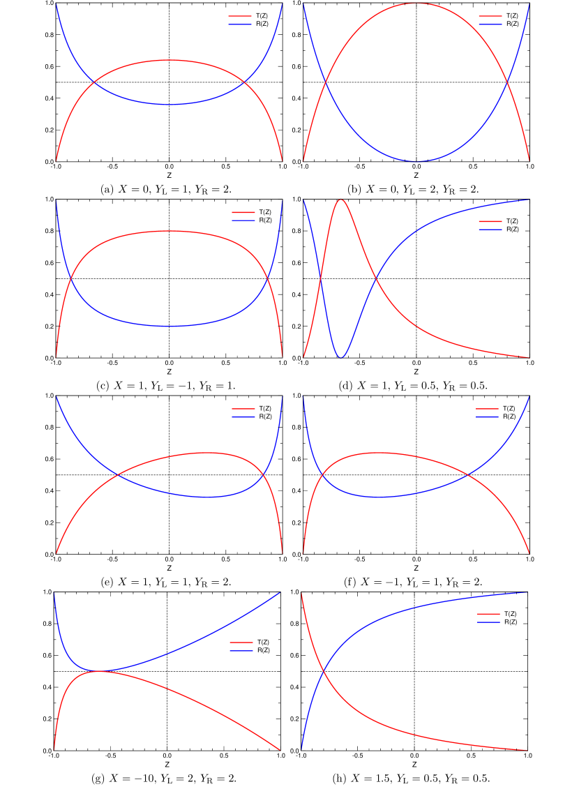
Figure 4: Graphic representations of the transmittance and reflectance for the resonant level system, as a function of energy, for different values of the parameters $X$, $Y_{\mathrm{L}}$ and $Y_{\mathrm{R}}$.

3 Transmittance through a benzene ring

We now turn to the central part of this work, where using the formalism above we compute the electronic transmittance through a benzene ring. Also the local density of states at the different carbon atoms of the ring is given.

In order to do so, we start by defining the system we shall study. It is quite similar to the level resonant system, but now the defect in not a different atom from the rest of the chain, but a benzene molecule connecting the two 1D chains, as represented in figure 5. These chains are equivalent to the ones presented before, and the hopping energies both on the chains and around the defect are equal as well. However, now the defect is composed by a benzene molecule, with all the carbon atoms placed at a distance $a$ from its nearest neighbours, and the hopping energy between these atoms being $-t_{\mathrm{b}}$. We also consider on-site energies in the positions of every atom of the benzene molecule, all of them with the value $-\varepsilon_{0}$. This makes the model more realistic, since there is a priori no particular reason for the on-site energy in the leads be equal to that in the benzene.

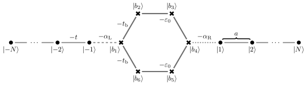
Figure 5: Schematic representation of the benzene system considered. This system is composed of two 1D chains with $N$ atoms each, represented by circles, and a benzene molecule in the middle of them. In this figure are also identified the hopping energies between different atoms ($-t$, $-t_{\mathrm{b}}$, $-\alpha_{\mathrm{L}}$ or $-\alpha_{\mathrm{R}}$, accordingly), the site energy on the atoms of the benzene ($-\varepsilon_{0}$) and the distance between two neighbours ($a$).

The Hamiltonian of the given system can be written as

$$H=H_{\mathrm{L}}+H_{\mathrm{C}}+H_{\mathrm{R}}+V\equiv H_{0}+V,$$ (53)

with

$$H_{\mathrm{L}}=-t\sum_{n=-N}^{-2}\Big{(}\left|n\right>\left<n+1\right|+\left|n+1\right>\left<n\right|\Big{)},$$ (54)

$$H_{\mathrm{C}}=\sum_{i=1}^{6}\Big{[}-t_{\mathrm{b}}\Big{(}\left|b_{i}\right>\left<b_{i+1}\right|+\left|b_{i+1}\right>\left<b_{i}\right|\Big{)}-\varepsilon_{0}\left|b_{i}\right>\left<b_{i}\right|\Big{]},$$ (55)

$$H_{\mathrm{R}}=-t\sum_{n=1}^{N-1}\Big{(}\left|n\right>\left<n+1\right|+\left|n+1\right>\left<n\right|\Big{)}$$ (56)

and

$$V=-\alpha_{\mathrm{L}}\Big{(}\left|-1\right>\left<b_{1}\right|+\left|b_{1}\right>\left<-1\right|\Big{)}-\alpha_{\mathrm{R}}\Big{(}\left|b_{4}\right>\left<1\right|+\left|1\right>\left<b_{4}\right|\Big{)},$$ (57)

where, due to the cyclic structure of the benzene molecule, $\left|b_{i+6}\right>=\left|b_{i}\right>$.

Considering now, as before, a flux incoming from the left of the defect, then (21) is still valid. On the other hand, the 1D chains surrounding the benzene molecule are similar as the ones considered in the previous example, which means that (30), (31), (33) and (34) are also still valid. As a consequence, the same is true for (32), for $n<0$, and zero otherwise. With this result, we can use the Lippmann-Schwinger equation, as given in (7), and proceed the same way as before, obtaining

$$\left<n\middle|\psi\right>= \sqrt{\frac{2}{N+1}}\sin\left(kan\right)-\alpha_{\mathrm{L}}\left<n\middle|G\middle|b_{1}\right>\sqrt{\frac{2}{N+1}}\sin\left(-ka\right), n<0$$ , (58)

$$\left<n\middle|\psi\right>= -\alpha_{\mathrm{L}}\left<n\middle|G\middle|b_{1}\right>\sqrt{\frac{2}{N+1}}\sin\left(-ka\right), n>0$$ . (59)

We must now find the matrix element $\left<n\middle|G\middle|b_{1}\right>$ of the operator $G$. Using the Dyson equation, and considering that, in the cases in which $n\neq b_{1,...,6}$, $\left<n\middle|G_{0}\middle|m\right>$ is only non-zero if $n$ and $m$ are both positive or both negative, we get

$$\left<n\middle|G\middle|b_{1}\right>= -\alpha_{\mathrm{L}}\left<n\middle|G_{0}\middle|-1\right>\left<b_{1}\middle|G\middle|b_{1}\right>, n<0$$ , (60)

$$\left<n\middle|G\middle|b_{1}\right>= -\alpha_{\mathrm{R}}\left<n\middle|G_{0}\middle|1\right>\left<b_{4}\middle|G\middle|b_{1}\right>, n>0$$ , (61)

We need now to calculate the matrix elements $\left<n\middle|G_{0}\middle|-1\right>$, $\left<n\middle|G_{0}\middle|1\right>$, $\left<b_{1}\middle|G\middle|b_{1}\right>$ and $\left<b_{4}\middle|G\middle|b_{1}\right>$. Due to the higher complexity of this case, we start now by the calculation of the matrix elements of $G_{0}$ instead of the ones of $G$, as done in the previous example. To do so, we use the result obtained in B,

$$G_{0}(n,m)= \frac{i}{2t\sqrt{1-\left(\frac{E}{2t}\right)^{2}}}\left(e^{ika\left|n+m\right|}-e^{ika\left|n-m\right|}\right), n\times m>0$$ , (62)

$$G_{0}(n,m)= \frac{1}{6}\sum_{l=1}^{6}\frac{e^{2\pi i\frac{l(n-m)}{6}}}{E+\varepsilon_{0}+2t_{\mathrm{b}}\cos\left(\frac{2\pi l}{6}\right)}, n,m=b_{i,j}$$ , (63)

$$G_{0}(n,m)= 0,$$ otherwise, (64)

where $i,j=1,\dots,6$, from where we find

$$\left<n\middle|G_{0}\middle|-1\right>=-\frac{e^{-ikan}}{t}$$ (65)

and

$$\left<n\middle|G_{0}\middle|1\right>=-\frac{e^{ikan}}{t}.$$ (66)

Through these results, we get

$$\left<n\middle|\psi\right>= \sqrt{\frac{2}{N+1}}\left[\frac{e^{ikan}}{2i}+\frac{e^{-ikan}}{2i}\left(-1+2iY_{\mathrm{L}}^{2}\sqrt{1-Z^{2}}t\left<b_{1}\middle|G\middle|b_{1}\right>\right)\right], n<0$$ , (67)

$$\left<n\middle|\psi\right>= \sqrt{\frac{2}{N+1}}\frac{e^{ikan}}{2i}\left[2iY_{\mathrm{L}}Y_{\mathrm{R}}\sqrt{1-Z^{2}}t\left<b_{4}\middle|G\middle|b_{1}\right>\right], n>0$$ . (68)

Finally, we only need the elements $\left<b_{1}\middle|G\middle|b_{1}\right>$ and $\left<b_{4}\middle|G\middle|b_{1}\right>$. These elements can be calculated through the system

$$\left<b_{1}\middle|G\middle|b_{1}\right>=\left<b_{1}\middle|G_{0}\middle|b_{1}\right>-\alpha_{\mathrm{L}}\left<b_{1}\middle|G_{0}\middle|b_{1}\right>\left<-1\middle|G\middle|b_{1}\right>-\alpha_{\mathrm{R}}\left<b_{1}\middle|G_{0}\middle|b_{4}\right>\left<1\middle|G\middle|b_{1}\right>,$$ (69)

$$\left<b_{4}\middle|G\middle|b_{1}\right>=\left<b_{4}\middle|G_{0}\middle|b_{1}\right>-\alpha_{\mathrm{L}}\left<b_{4}\middle|G_{0}\middle|b_{1}\right>\left<-1\middle|G\middle|b_{1}\right>-\alpha_{\mathrm{R}}\left<b_{4}\middle|G_{0}\middle|b_{4}\right>\left<1\middle|G\middle|b_{1}\right>,$$ (70)

$$\left<-1\middle|G\middle|b_{1}\right>=-\alpha_{\mathrm{L}}\left<-1\middle|G_{0}\middle|-1\right>\left<b_{1}\middle|G\middle|b_{1}\right>$$ (71)

$$\left<1\middle|G\middle|b_{1}\right>=-\alpha_{\mathrm{R}}\left<1\middle|G_{0}\middle|1\right>\left<b_{4}\middle|G\middle|b_{1}\right>,$$ (72)

where all equations were derived from the Dyson equation. It follows that, defining $G_{n,m}\equiv\left<n\middle|G\middle|m\right>$ and $G^{0}_{n,m}\equiv\left<n\middle|G_{0}\middle|m\right>$, we get

$$G_{b_{1},b_{1}}=\frac{G^{0}_{b_{1},b_{1}}+\alpha_{\mathrm{R}}^{2}G^{0}_{1,1}\left(G^{0}_{b_{1},b_{4}}G^{0}_{b_{4},b_{1}}-G^{0}_{b_{1},b_{1}}G^{0}_{b_{4},b_{4}}\right)}{1-\alpha_{\mathrm{L}}^{2}G^{0}_{-1,-1}G^{0}_{b_{1},b_{1}}-\alpha_{\mathrm{R}}^{2}G^{0}_{1,1}G^{0}_{b_{4},b_{4}}-\alpha_{\mathrm{L}}^{2}\alpha_{\mathrm{R}}^{2}G^{0}_{-1,-1}G^{0}_{1,1}\left(G^{0}_{b_{1},b_{4}}G^{0}_{b_{4},b_{1}}-G^{0}_{b_{1},b_{1}}G^{0}_{b_{4},b_{4}}\right)}$$ (73)

and

$$G_{b_{4},b_{1}}=\frac{G^{0}_{b_{4},b_{1}}}{1-\alpha_{\mathrm{L}}^{2}G^{0}_{-1,-1}G^{0}_{b_{1},b_{1}}-\alpha_{\mathrm{R}}^{2}G^{0}_{1,1}G^{0}_{b_{4},b_{4}}-\alpha_{\mathrm{L}}^{2}\alpha_{\mathrm{R}}^{2}G^{0}_{-1,-1}G^{0}_{1,1}\left(G^{0}_{b_{1},b_{4}}G^{0}_{b_{4},b_{1}}-G^{0}_{b_{1},b_{1}}G^{0}_{b_{4},b_{4}}\right)}.$$ (74)

To close the problem, we only need some matrix elements of $G_{0}$, which can be found using again the result from equation (64). Doing so, and defining $\Upsilon\equiv{t_{\mathrm{b}}}/{t}$, we get

$$G^{0}_{-1,-1}=G^{0}_{1,1}=-\frac{e^{ika}}{t}=\frac{1}{t}\left[Z-i\sqrt{1-Z^{2}}\right],$$ (75)

$$G^{0}_{b_{1},b_{1}}=G^{0}_{b_{4},b_{4}}=\frac{1}{t}\left\{\frac{-\frac{1}{2\Upsilon^{3}}\left(Z+\frac{X}{2}\right)\left[\frac{1}{\Upsilon^{2}}\left(Z+\frac{X}{2}\right)^{2}-3\right]}{\left[\frac{1}{\Upsilon^{2}}\left(Z+\frac{X}{2}\right)^{2}-1\right]\left[\frac{4}{\Upsilon^{2}}\left(Z+\frac{X}{2}\right)^{2}-1\right]}\right\},$$ (76)

and

$$G^{0}_{b_{4},b_{1}}=G^{0}_{b_{1},b_{4}}=\frac{1}{t}\left\{\frac{\frac{1}{2\Upsilon}}{\left[\frac{1}{\Upsilon^{2}}\left(Z+\frac{X}{2}\right)^{2}-1\right]\left[\frac{4}{\Upsilon^{2}}\left(Z+\frac{X}{2}\right)^{2}-1\right]}\right\}.$$ (77)

Note that all these elements are only numbers (real or complex), that are function of the energy and several other parameters, but not the position $n$. As a consequence, the same is true for the elements $G_{b_{1},b_{1}}$ and $G_{b_{4},b_{1}}$. This means that we find

$$r=2iY_{\mathrm{L}}^{2}\sqrt{1-Z^{2}}\left[tG_{b_{1},b_{1}}\right]-1,$$ (78)

$$\tau=2iY_{\mathrm{L}}Y_{\mathrm{R}}\sqrt{1-Z^{2}}\left[tG_{b_{4},b_{1}}\right],$$ (79)

and, finally,

$$\mathcal{R}=1+4Y_{\mathrm{L}}^{4}\left(1-Z^{2}\right)t^{2}\left|G_{b_{1},b_{1}}\right|^{2}+4Y_{\mathrm{L}}^{2}\sqrt{1-Z^{2}}\mathrm{Im}\left[tG_{b_{1},b_{1}}\right],$$ (80)

$$\mathcal{T}=4\left(Y_{\mathrm{L}}Y_{\mathrm{R}}\right)^{2}\left(1-Z^{2}\right)t^{2}\left|G_{b_{4},b_{1}}\right|^{2}.$$ (81)

In figure 6, we present some graphical representations of $\mathcal{R}$ and $\mathcal{T}$ as function of the energy $Z$, for several combinations of the parameters $X$, $\Upsilon$, $Y_{\mathrm{L}}$ and $Y_{\mathrm{R}}$. The discussion of the results is left for the final section of the paper.

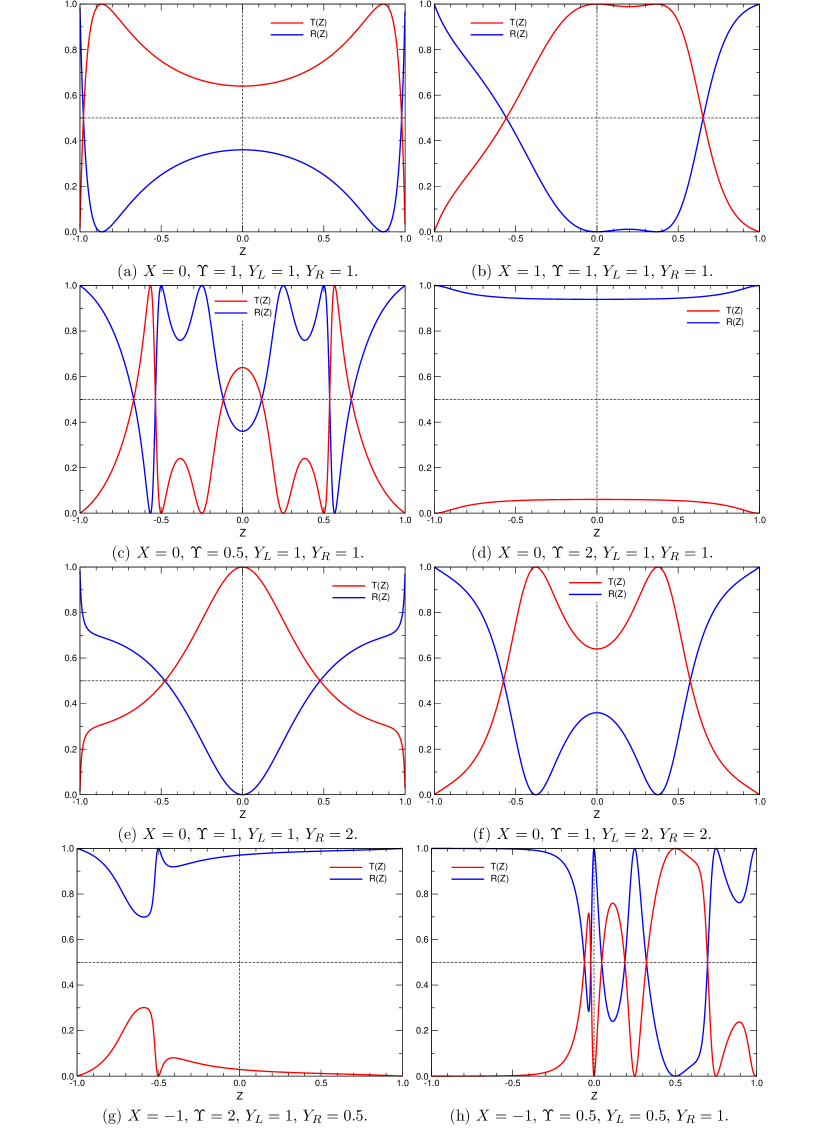
Figure 6: Graphic representations of the transmittance and reflectance through a benzene ring, as a function of energy, for different values of the parameters $X$, $\Upsilon$, $Y_{\mathrm{L}}$ and $Y_{\mathrm{R}}$.

3.1 Local Density of States

One of the main advantages of the Green’s function approach is that the calculation of the Local Density of States (LDOS) in the atom of the position $n$ is straightforward. It is given by [17]

$$\rho_{n}(Z)=-\frac{1}{\pi}\mathrm{Im}G_{n,n}(Z),$$ (82)

where $G_{n,n}\equiv\left<n\middle|G\middle|n\right>$. For the benzene system, we are interested in the LDOS in each of the atoms of the benzene ring. In general, it should be different for each atom except, due to the symmetry of the system, $\rho_{b_{2}}(Z)=\rho_{b_{6}}(Z)$ and $\rho_{b_{3}}(Z)=\rho_{b_{5}}(Z)$. In the particular case when $\alpha_{\mathrm{L}}=\alpha_{\mathrm{R}}$, there is a higher level of symmetry which imposes that $\rho_{b_{2}}(Z)=\rho_{b_{3}}(Z)=\rho_{b_{5}}(Z)=\rho_{b_{6}}(Z)$ and also $\rho_{b_{1}}(Z)=\rho_{b_{4}}(Z)$.

To calculate each of this different local densities of states, we need to find the matrix elements $\left<b_{n}\middle|G\middle|b_{n}\right>$, with $n=1,...,6$. Through Dyson equation, we find

$$\left<b_{n}\middle|G\middle|b_{n}\right>=\left<b_{n}\middle|G_{0}\middle|b_{n}\right>-\alpha_{\mathrm{L}}\left<b_{n}\middle|G_{0}\middle|b_{1}\right>\left<-1\middle|G\middle|b_{n}\right>-\alpha_{\mathrm{R}}\left<b_{n}\middle|G_{0}\middle|b_{4}\right>\left<1\middle|G\middle|b_{n}\right>,$$ (83)

$$\left<-1\middle|G\middle|b_{n}\right>=-\alpha_{\mathrm{L}}\left<-1\middle|G_{0}\middle|-1\right>\left<b_{1}\middle|G\middle|b_{n}\right>,$$ (84)

$$\left<1\middle|G\middle|b_{n}\right>=-\alpha_{\mathrm{R}}\left<1\middle|G_{0}\middle|1\right>\left<b_{4}\middle|G\middle|b_{n}\right>,$$ (85)

$$\left<b_{1}\middle|G\middle|b_{n}\right>=\left<b_{1}\middle|G_{0}\middle|b_{n}\right>-\alpha_{\mathrm{L}}\left<b_{1}\middle|G_{0}\middle|b_{1}\right>\left<-1\middle|G\middle|b_{n}\right>-\alpha_{\mathrm{R}}\left<b_{1}\middle|G_{0}\middle|b_{4}\right>\left<1\middle|G\middle|b_{n}\right>,$$ (86)

$$\left<b_{4}\middle|G\middle|b_{n}\right>=\left<b_{4}\middle|G_{0}\middle|b_{n}\right>-\alpha_{\mathrm{L}}\left<b_{4}\middle|G_{0}\middle|b_{1}\right>\left<-1\middle|G\middle|b_{n}\right>-\alpha_{\mathrm{R}}\left<b_{4}\middle|G_{0}\middle|b_{4}\right>\left<1\middle|G\middle|b_{n}\right>.$$ (87)

These five equations make up a closed system from where it is possible to find the value of $\left<b_{n}\middle|G\middle|b_{n}\right>$. However, the analytic solutions, although possible to find, are too complex to have any interest in being presented. As an alternative, we present, in figure 7, graphical representations of the LDOS in each atom, as function of the energy $Z$, for several combinations of the parameters $X$, $\Upsilon$, $Y_{\mathrm{L}}$ and $Y_{\mathrm{R}}$. From the study of this figure it is clear that the behaviour of the LDOS is rather complex, depending on the actual values of the parameters.

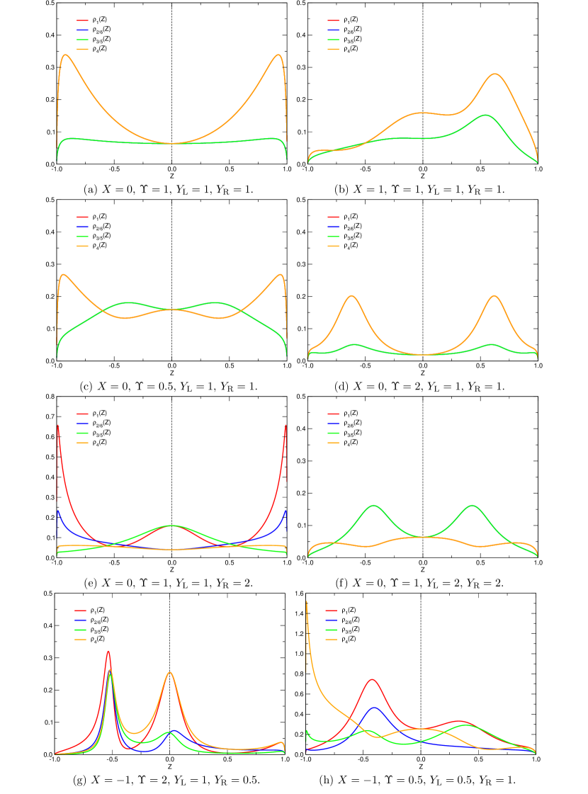
Figure 7: Graphic representations of the local density of states in the atoms of a benzene ring, as a function of energy, for different values of the parameters $X$, $\Upsilon$, $Y_{\mathrm{L}}$ and $Y_{\mathrm{R}}$. Note that, in figures (a)–(d) and (f), the red and orange lines are superimposed, as well as the blue and green ones.

4 Discussion

In conclusion, we have developed a formalism, based on Green’s functions, for describing the electronic transport through molecules represented by tight-binding models. We started by explaining the general method, defining some useful operators. To illustrate its usage, we then applied it to the case of the resonant level system, where we were able to find its transmittance. To do so, we also found the wave functions and the allowed energies of electrons propagating in an ideal unidimensional chain. From the expressions found for the transmittance and reflectance of this system, and the subsequent presented plots, we draw a number of useful results:

• both $\mathcal{T}$ and $\mathcal{R}$ are symmetrical with respect to the line $\mathcal{T}=\mathcal{R}=0.5$. This is due to the condition $\mathcal{T}+\mathcal{R}=1$;

• in most cases, at $Z=\pm 1$, we found that $\mathcal{T}=0$ and $\mathcal{R}=1$. The exception was the plot presented in figure 4(h), in which $\mathcal{T}=1$ and $\mathcal{R}=0$ at $Z=1$. Through an analysis of the limits of (51), we found that this exceptions occur whenever one set of parameters respects the condition $\left|X/2\right|=\left|(Y_{\mathrm{L}}^{2}+Y_{\mathrm{R}}^{2})/2-1\right|$ [which is the case of the parameters in figure 4(h)]. In these cases, the transmittance is total in at least one of the extremes of the band;

• when $X=0$, the these functions are also symmetrical with respect to $Z=0$. This means that they must have a maximum or minimum at this energy. On the other hand, when $X$ was a positive (negative) number, the peak tended to slide to the right (left), for the same parameters $Y_{\mathrm{L}}$ and $Y_{\mathrm{R}}$. Analysing (51), we found that the extreme of these functions depends on the other parameters through the expression

  $$Z_{\mathrm{extremo}}= \frac{\frac{X}{2}}{\frac{Y_{\mathrm{L}}^{2}+Y_{\mathrm{R}}^{2}}{2}-1}, \left|\frac{X}{2}\right|\leq\left|\frac{Y_{\mathrm{L}}^{2}+Y_{\mathrm{R}}^{2}}{2}-1\right|$$ , (88)

  $$Z_{\mathrm{extremo}}= \frac{\frac{Y_{\mathrm{L}}^{2}+Y_{\mathrm{R}}^{2}}{2}-1}{\frac{X}{2}}, \left|\frac{X}{2}\right|>\left|\frac{Y_{\mathrm{L}}^{2}+Y_{\mathrm{R}}^{2}}{2}-1\right|$$ . (89)

  This result explains both the behaviour of the peak with a change in $X$ and also the exception presented in the previous point;

• through the two previous points, we conclude that the extreme found must be a maximum of the transmittance and a minimum of the reflectance. Using (51), we obtain that [19]

  $$\mathcal{T}_{\mathrm{max}}= \frac{4Y_{\mathrm{L}}^{2}Y_{\mathrm{R}}^{2}}{\left(Y_{\mathrm{L}}^{2}+Y_{\mathrm{R}}^{2}\right)^{2}}, \left|\frac{X}{2}\right|\leq\left|\frac{Y_{\mathrm{L}}^{2}+Y_{\mathrm{R}}^{2}}{2}-1\right|$$ , (90)

  $$\mathcal{T}_{\mathrm{max}}= \frac{Y_{\mathrm{L}}^{2}Y_{\mathrm{R}}^{2}}{\left(\frac{X}{2}\right)^{2}+Y_{\mathrm{L}}^{2}+Y_{\mathrm{R}}^{2}-1}, \left|\frac{X}{2}\right|>\left|\frac{Y_{\mathrm{L}}^{2}+Y_{\mathrm{R}}^{2}}{2}-1\right|$$ . (91)

  In particular, when $Y_{\mathrm{L}}=Y_{\mathrm{R}}\equiv Y$, we get the important result

  $$\mathcal{T}_{\mathrm{max}}= 1, \left|\frac{X}{2}\right|\leq\left|Y^{2}-1\right|$$ , (92)

  $$\mathcal{T}_{\mathrm{max}}= \frac{Y^{4}}{\left(\frac{X}{2}\right)^{2}+2Y^{2}-1}, \left|\frac{X}{2}\right|>\left|Y^{2}-1\right|$$ . (93)

  This result is important because, as we can see, when $Y_{\mathrm{L}}=Y_{\mathrm{R}}$, we can adjust the parameters $X$ and $Y$ so that, at some energy, we have maximum transmittance. This is not possible when $Y_{\mathrm{L}}\neq Y_{\mathrm{R}}$, nor in the simplest case of point defect in which $Y_{\mathrm{L}}=Y_{\mathrm{R}}=1$. This is why this problem is called the level resonant system. In the diagram of figure 8, the region of the phase space $XY$ where $\mathcal{T}_{\mathrm{max}}=1$ is presented in grey. On the other hand, in the white region of the same diagram, the maximum transmittance is always lower than one, decreasing with the distance to the bold line defined by $\left|X/2\right|=\left|Y^{2}-1\right|$. To understand the topology of this region, some level lines are represented;

  

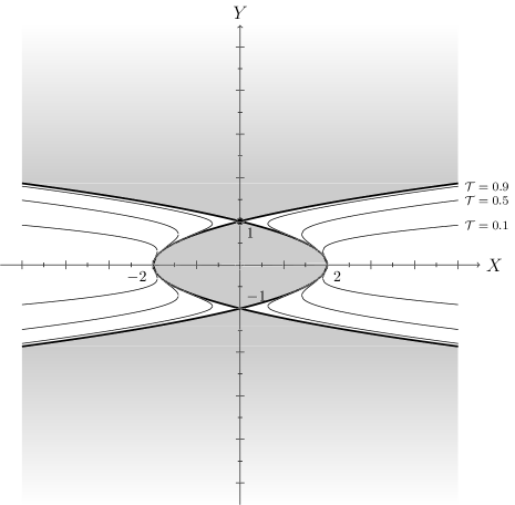
  Figure 8: This diagram shows: in a bold line, the points for which $\left|X/2\right|=\left|Y^{2}-1\right|$; in a grey shadow, the region of the phase space $XY$ where $\mathcal{T}_{\mathrm{max}}=1$; in white, the region where $\mathcal{T}_{\mathrm{max}}<1$; in thin lines, some level lines, for $\mathcal{T}_{\mathrm{max}}=0.1$, $\mathcal{T}_{\mathrm{max}}=0.5$ and $\mathcal{T}_{\mathrm{max}}=0.9$; and a black dot which represents the point in the phase space corresponding to the ideal system, that is, $Y=1$ and $X=0$. The grey shaded region continues as $Y\rightarrow\pm\infty$. Note that the diagram is symmetrical both with respect to the lines $X=0$ and $Y=0$.

• in the general case, for the same $Y_{\mathrm{L}}$ and $Y_{\mathrm{R}}$, the transmittance increases with the decreasing of $X$, as expected, but only when $\left|X/2\right|>\left|(Y_{\mathrm{L}}^{2}+Y_{\mathrm{R}}^{2})/2-1\right|$. Elsewhere, this value is independent of $X$. On the other hand, for the same $X$, the transmittance tends to increase when $Y_{\mathrm{L}}=Y_{\mathrm{R}}$ and also when $Y_{\mathrm{L}}$ and $Y_{\mathrm{R}}$, as represented in the phase space $XY_{\mathrm{L}}Y_{\mathrm{R}}$, get closer to the surface defined by $\left|X/2\right|=\left|(Y_{\mathrm{L}}^{2}+Y_{\mathrm{R}}^{2})/2-1\right|$, and decrease with the distance to that surface. In particular, it is null when either $Y_{\mathrm{L}}$ or $Y_{\mathrm{R}}$ are null.

We then studied the case of the benzene system, and presented plots of its transmittance and reflectance, for different sets of parameters. Here, the plots obtained for the transmittance were much more complex, depending on four parameters, which means that a study like the one presented for the resonant level system above is much more difficult to elaborate. Indeed, It would require an extensive study of the limits of the transmittance and reflectance for several values of the presented parameters, and also the production of much more plots than the ones presented here, what would worth of paper of itself. Our goal was rather to show that the Green’s function method an easily be applied to a problem of moderate difficulty. The same can be said about the local density of states in each atom of the benzene ring, which was also calculated in this paper.

Nevertheless, some qualitative aspects can be drawn from the results of Fig. 6. Taking the single example of panel (h) of that figure we seen that the transmittance is strongly suppressed for values of the energy such that $Z<-0.5$. If we now imagine that the energy of the electrons can be tuned, such a system would correspond to an electronic filter, where only the electrons with energies in the range $-0.5<Z<0$ would be transmitted. The same can be said for the results in panel (g) and energies $Z>0$.

This method, as should now be clear, can be easily generalized to more complex problems, such as a chain of atoms, like a polyacetylene, or two (or more) benzene rings in a row. However, we can conclude that the analytical expressions of the found quantities, although possible to find through this method, can get rather complex when the complexity of the problem increases, due to the increase of the number of atoms involved in the calculation. In this case, the method can be formulated using efficient numerical methods.

In synthesis, as should now be obvious, the Green’s functions method is ideal for tackling transport problems in molecular electronics, providing, in many cases, analytical expressions for the quantum transmittance, which can further be analysed in detail for the benefit of gaining insight on the transport properties of a given system.

Appendix A Matrix elements of the free Green’s operator for the resonant level system

In this appendix, we present the calculation of the matrix elements $G_{0}(n,m)$ of the free Green’s function operator for the resonant level system. These elements are given by

$$G_{0}(n,m)=\left<n\middle|G_{0}\middle|m\right> =\left<n\right|\frac{1}{E-H_{0}+i\epsilon}\left|m\right>$$ (94)

where $H_{0}=H_{\mathrm{L}}+H_{\mathrm{C}}+H_{\mathrm{R}}$, defined as in (16)–(18). We start by using a Taylor expansion of the form $1/(x_{0}-x)=\sum_{l=0}^{+\infty}x^{l}/x_{0}^{l+1}$, so that

$$G_{0}(n,m) =\sum_{l=0}^{+\infty}\left<n\right|\frac{\left(H_{\mathrm{L}}+H_{\mathrm{C}}+H_{\mathrm{R}}\right)^{l}}{\left(E+i\epsilon\right)^{l+1}}\left|m\right>.$$ (95)

The subsequent expansion of the power in the numerator, for any $l$, will mix the different components of $H_{0}$ in many possible combinations. However, since the three components $H_{\mathrm{L}}$, $H_{\mathrm{C}}$ and $H_{\mathrm{R}}$ are uncoupled, any operator operating in a position state of a different region will vanish (and, once these particular operators are Hermitian, this is valid for both the bra and the ket surrounding it), remaining only

$$G_{0}(n,m)= \sum_{l=0}^{+\infty}\frac{\left<n\middle|H_{\mathrm{L}}^{l}\middle|m\right>}{\left(E+i\epsilon\right)^{l+1}}=\left<n\right|\frac{1}{E-H_{\mathrm{L}}+i\epsilon}\left|m\right>\equiv\left<n\right|G_{\mathrm{L}}\left|m\right>, n,m<0$$ , (96)

$$G_{0}(n,m)= \sum_{l=0}^{+\infty}\frac{\left<n\middle|H_{\mathrm{C}}^{l}\middle|m\right>}{\left(E+i\epsilon\right)^{l+1}}=\left<n\right|\frac{1}{E-H_{\mathrm{C}}+i\epsilon}\left|m\right>\equiv\left<n\right|G_{\mathrm{C}}\left|m\right>, n,m=0$$ , (97)

$$G_{0}(n,m)= \sum_{l=0}^{+\infty}\frac{\left<n\middle|H_{\mathrm{R}}^{l}\middle|m\right>}{\left(E+i\epsilon\right)^{l+1}}=\left<n\right|\frac{1}{E-H_{\mathrm{R}}+i\epsilon}\left|m\right>\equiv\left<n\right|G_{\mathrm{R}}\left|m\right>, n,m>0$$ , (98)

$$G_{0}(n,m)= 0,$$ otherwise. (99)

As we can see now, the value of the matrix elements will, in general, be different for three different regions, so we shall now proceed to each calculation separately.

A.1 Calculation for the 1D chains next to the defect

Due to the high symmetry verified between the chains in both sides of the defect, these two cases will be treated simultaneously. In these regions, we ought to find the elements

$$G_{0}(n,m)= G_{\mathrm{L}}(n,m)=\left<n\middle|G_{\mathrm{L}}\middle|m\right>, n,m<0$$ , (100)

$$G_{0}(n,m)= G_{\mathrm{R}}(n,m)=\left<n\middle|G_{\mathrm{R}}\middle|m\right>, n,m>0$$ . (101)

where

$$G_{\mathrm{L}}=\frac{1}{E-H_{\mathrm{L}}+i\epsilon},$$ (102)

$$G_{\mathrm{R}}=\frac{1}{E-H_{\mathrm{R}}+i\epsilon}.$$ (103)

Back in section 2, the eigenstates of $H_{\mathrm{L}}$ and $H_{\mathrm{R}}$ were found, and are presented in (31) and (34). Since each of them makes up a complete basis, we can use the notation $\left|\psi_{\mathrm{L}}\right>\equiv\left|k_{\mathrm{L}}\right>$ and $\left|\psi_{\mathrm{R}}\right>\equiv\left|k_{\mathrm{R}}\right>$ to write

$$\mathbb{I} =\sum_{k}\left|k_{\mathrm{L}}\right>\left<k_{\mathrm{L}}\right|=\sum_{k}\left|k_{\mathrm{R}}\right>\left<k_{\mathrm{R}}\right|$$ (104)

where $\mathbb{I}$ is the unity operator and the sums are over all allowed values of $k$. With this result, the matrix elements can be written as

$$G_{0}(n,m)= \sum_{k}\left<n\middle|k_{\mathrm{L}}\right>\left<k_{\mathrm{L}}\middle|G_{\mathrm{L}}\middle|m\right>=\sum_{k}\sum_{l=0}^{+\infty}\frac{\left<k_{\mathrm{L}}\middle|H_{\mathrm{L}}^{l}\middle|m\right>}{\left(E+i\epsilon\right)^{l+1}}\left<n\middle|k_{\mathrm{L}}\right>, n,m<0$$ , (105)

$$G_{0}(n,m)= \sum_{k}\left<n\middle|k_{\mathrm{R}}\right>\left<k_{\mathrm{R}}\middle|G_{\mathrm{R}}\middle|m\right>=\sum_{k}\sum_{l=0}^{+\infty}\frac{\left<k_{\mathrm{R}}\middle|H_{\mathrm{R}}^{l}\middle|m\right>}{\left(E+i\epsilon\right)^{l+1}}\left<n\middle|k_{\mathrm{R}}\right>, n,m>0$$ . (106)

The advantage of writing these elements as such is that $H_{\mathrm{L}}^{l}\left|k_{\mathrm{L}}\right>=E(k)^{l}\left|k_{\mathrm{L}}\right>$, with $E(k)$ defined in (33). The same is true for $\left|k_{\mathrm{R}}\right>$ and $H_{\mathrm{R}}$. Through this result, the previous expression simplifies to

$$G_{0}(n,m)= \sum_{k}\frac{\left<n\middle|k_{\mathrm{L}}\right>\left<k_{\mathrm{L}}\middle|m\right>}{E+2t\cos\left(ka\right)+i\epsilon}, n,m<0$$ , (107)

$$G_{0}(n,m)= \sum_{k}\frac{\left<n\middle|k_{\mathrm{R}}\right>\left<k_{\mathrm{R}}\middle|m\right>}{E+2t\cos\left(ka\right)+i\epsilon}, n,m>0$$ . (108)

Now, if we recall (30), we see that $\Delta k\equiv k_{n+1}-k_{n}=\pi\left[a\left(N+1\right)\right]^{-1}$. When $N\gg 1$, then $\Delta k$ tends to an infinitesimal element $dk$, and thus, if we multiply (and divide) the previous equations by $\Delta k$, we can approximate the sum to an integral. Moreover, we already know the value of the operations $\left<n\middle|k\right>$ and $\left<k\middle|n\right>$ ($k=k_{\mathrm{L}},k_{\mathrm{R}}$). Through these two results, we find that, for both sides of the defect, the matrix elements of $G_{0}$ are given by

$$G_{0}(n,m) =\frac{1}{\Delta k}\frac{2}{N+1}\int_{0}^{\frac{\pi}{a}}dk\frac{\sin\left(kan\right)\sin\left(kam\right)}{E+2t\cos\left(ka\right)+i\epsilon}$$ (109)

$$=\frac{2a}{\pi}\frac{1}{2}\int_{-\frac{\pi}{a}}^{\frac{\pi}{a}}dk\frac{\sin\left(kan\right)\sin\left(kam\right)}{E+2t\cos\left(ka\right)+i\epsilon},$$ (110)

where we noted that the function being integrated is even. This expression is now valid when $n,m>0$ or $n,m<0$, or, to simplify, when $n\times m>0$. Writing now the sine functions in the Euler notation, we get

$$G_{0}(n,m)=-\frac{a}{4\pi}\int_{-\frac{\pi}{a}}^{\frac{\pi}{a}}dk\frac{e^{ika(n+m)}-e^{ika(n-m)}+e^{-ika(n+m)}-e^{-ika(n-m)}}{E+2t\cos\left(ka\right)+i\epsilon}.$$ (111)

However, due to the parity of the functions sine and cosine that make up each complex exponential in the previous equation, we verify that the integration of the terms whose numerator is $e^{ika(n+m)}-e^{ika(n-m)}$ is equal to ones whose numerator is $e^{-ika(n+m)}-e^{-ika(n-m)}$, which means the integral can be rewritten in the simpler form

$$G_{0}(n,m) =-\frac{a}{4\pi}2\int_{-\frac{\pi}{a}}^{\frac{\pi}{a}}dk\frac{e^{ika\left|n+m\right|}-e^{ika\left|n-m\right|}}{E+2t\cos\left(ka\right)+i\epsilon}$$ (112)

$$=\frac{a}{2\pi}\left[\int_{-\frac{\pi}{a}}^{\frac{\pi}{a}}dk\frac{e^{ika\left|n-m\right|}}{E+2t\cos\left(ka\right)+i\epsilon}-\int_{-\frac{\pi}{a}}^{\frac{\pi}{a}}dk\frac{e^{ika\left|n+m\right|}}{E+2t\cos\left(ka\right)+i\epsilon}\right]$$ (113)

$$\equiv I(\left|n-m\right|)-I(\left|n+m\right|),$$ (114)

where

$$I(x)\equiv\frac{a}{2\pi}\int_{-\frac{\pi}{a}}^{\frac{\pi}{a}}dk\frac{e^{ikax}}{E+2t\cos\left(ka\right)+i\epsilon}.$$ (115)

Thus, we need now to find the general solution of $I(x)$ to find the matrix elements we need. The solution of this integral was found to be (see below)

$$I(x)=\frac{-ie^{ikax}}{2t\sqrt{1-\left(\frac{E}{2t}\right)^{2}}},$$ (116)

what means that the general result for the matrix elements of $G_{0}$, for $n\times m>0$, is

$$G_{0}(n,m)=\frac{i}{2t\sqrt{1-\left(\frac{E}{2t}\right)^{2}}}\left(e^{ika\left|n+m\right|}-e^{ika\left|n-m\right|}\right).$$ (117)

We need yet to prove the solution of the integral $I(x)$. Defining $\theta\equiv ka$ and $z=E+i\epsilon$, we rewrite the integral as

$$I(x)=\frac{1}{2\pi}\int_{-\pi}^{\pi}d\theta\frac{e^{i\theta x}}{z+t\left(e^{i\theta}+e^{-i\theta}\right)}.$$ (118)

Defining also $w\equiv e^{ix}$, the previous integral takes the form

$$I(x) =\frac{1}{2\pi}\oint_{\gamma}\frac{dw}{iw}\frac{w^{x}}{z+t(w+w^{-1})}$$ (119)

$$=\frac{1}{2\pi it}\oint_{\gamma}dw\frac{w^{x}}{w^{2}+\frac{wz}{t}+1}$$ (120)

$$=\frac{1}{2\pi it}\oint_{\gamma}dw\frac{w^{x}}{(w-w_{1})(w-w_{2})},$$ (121)

where $\gamma$ is an unitary circle in the complex plane and $w_{1}$ e $w_{2}$ are the two roots of $w^{2}+wz/t+1$, given by

$$w_{1,2}=-\frac{z}{2t}\pm i\sqrt{1-\left(\frac{z}{2t}\right)^{2}}$$ (122)

(where the subscript $1$ corresponds to the signal $+$, and vice versa). Note that we are interested in the case when $-2t<E<2t$ (what corresponds to the bandwidth of these chains). The integral in now written in such a way that it is now convenient to use the Residue Theorem. However, to do so, we need to know whether each singularity is contained in $\gamma$. That calculation is done in A.3, from where it was concluded that, when $\epsilon\to 0^{+}$, then ${w_{1}}\to 1^{-}$ and ${w_{2}}\to 1^{+}$. This means that

$$I(x) =\frac{1}{2\pi it}2\pi i\mathrm{Res}_{w=w_{1}}\left[\frac{w^{x}}{(w-w_{1})(w-w_{2})}\right]$$ (123)

$$=\frac{1}{t}\frac{w_{1}^{x}}{w_{1}-w_{2}},$$ (124)

where $\mathrm{Res}_{z=z_{0}}f(z)$ denotes the residue of $f(z)$ at $z=z_{0}$. Note now that, when $\epsilon\to 0$, we can use the relation $E=-2t\cos\left(ka\right)$ to write the singularities as

$$w_{1,2}=-\frac{E}{2t}\pm i\sqrt{1-\left(\frac{E}{2t}\right)^{2}}=e^{\pm ika}.$$ (125)

Through this result, we finally obtain the already stated result

$$I(x)=\frac{-ie^{ikax}}{2t\sqrt{1-\left(\frac{E}{2t}\right)^{2}}}.$$ (126)

A.2 Calculation for the defect

In this region, we need to find the elements

$$G_{\mathrm{C}}(n,m)=\left<n\middle|G_{\mathrm{C}}\middle|m\right>,$$ (127)

where

$$G_{\mathrm{C}}=\frac{1}{E-H_{\mathrm{C}}+i\epsilon},$$ (128)

and the Hamiltonian $H_{\mathrm{C}}$ was defined in (17). As was stated before, the only matrix element of $G_{\mathrm{C}}$ that does not vanish is $G_{\mathrm{C}}(0,0)$. This case is much simpler than the previous one, because the position state $\left|0\right>$ is already an eigenstate of $H_{\mathrm{C}}$, with $H_{\mathrm{C}}\left|0\right>=-\varepsilon_{0}\left|0\right>$. As such,

$$G_{0}(0,0) =\sum_{l=0}^{+\infty}\frac{\left<0\middle|H_{\mathrm{C}}^{l}\middle|0\right>}{\left(E+i\epsilon\right)^{l+1}}$$ (129)

$$=\sum_{l=0}^{+\infty}\frac{\left<0\middle|\left(-\varepsilon_{0}\right)^{l}\middle|0\right>}{\left(E+i\epsilon\right)^{l+1}}$$ (130)

$$\rightarrow\frac{1}{E+\varepsilon_{0}},$$ (131)

when $\epsilon\to 0$.

In short, the matrix elements of $G_{0}$ for the resonant level system are

$$G_{0}(n,m)= \frac{1}{E+\varepsilon_{0}}, n=m=0$$ , (132)

$$G_{0}(n,m)= \frac{i}{2t\sqrt{1-\left(\frac{E}{2t}\right)^{2}}}\left(e^{ika\left|n+m\right|}-e^{ika\left|n-m\right|}\right), n\times m>0$$ , (133)

$$G_{0}(n,m)= 0,$$ otherwise. (134)

A.3 Evaluation of the absolute value of the singularities found

In this appendix, we will evaluate the absolute value of the complex numbers $w_{1,2}$, defined in (122). Let us consider that $\epsilon$ is so small that

$$\epsilon^{2}=0,$$ (135)

$$x\epsilon=\mathrm{sgn}\left(x\right)\epsilon$$ (136)

and, as a particular case of the previous,

$$\epsilon+\epsilon=\epsilon,$$ (137)

where $x$ is some real number and the signal function is defined as

$$\mathrm{sgn}\left(x\right)= +1, x>0$$ , (138)

$$\mathrm{sgn}\left(x\right)= 0, x=0$$ , (139)

$$\mathrm{sgn}\left(x\right)= -1, x<0$$ . (140)

Expanding now the squared binomial expression present in (122), and noting the previous considerations, we get

$$w_{1,2} =-\left(\frac{E+i\epsilon}{2t}\right)\pm\sqrt{\left(\frac{E}{2t}\right)^{2}-1+i\mathrm{sgn}\left(E\right)\epsilon}$$ (141)

$$=-\left(\frac{E+i\epsilon}{2t}\right)\pm\sqrt{\left[1-\left(\frac{E}{2t}\right)^{2}\right]\left[-1+i\mathrm{sgn}\left(E\right)\epsilon\right]}$$ (142)

$$=-\left(\frac{E+i\epsilon}{2t}\right)\pm i\sqrt{1-\left(\frac{E}{2t}\right)^{2}}\sqrt{1-i\mathrm{sgn}\left(E\right)\epsilon}.$$ (143)

Since $\epsilon$ is as small as necessary, we can use a first order Taylor approximation of the function $\sqrt{1-x}$ at $x\approx 0$, with the result $\sqrt{1+x}\approx 1+{x}/{2}$. Doing so, the previous expression simplifies to

$$w_{1,2} =-\left(\frac{E+i\epsilon}{2t}\right)\pm i\sqrt{1-\left(\frac{E}{2t}\right)^{2}}\left[1-i\mathrm{sgn}\left(E\right)\epsilon\right]$$ (144)

$$=-\left[\frac{E}{2t}\mp\mathrm{sgn}\left(E\right)\epsilon\right]-i\left[\mp\sqrt{1-\left(\frac{E}{2t}\right)^{2}}+\epsilon\right].$$ (145)

Consider now the squared absolute value $w_{1,2}$, given by $\left|w_{1,2}\right|^{2}=w_{1,2}w_{1,2}^{*}$. Through this expression,

$$\left|w_{1,2}\right|^{2} =\left[\frac{E}{2t}\mp\mathrm{sgn}\left(E\right)\epsilon\right]^{2}+\left[\mp\sqrt{1-\left(\frac{E}{2t}\right)^{2}}+\epsilon\right]^{2}$$ (146)

$$=\left[\left(\frac{E}{2t}\right)^{2}\mp\mathrm{sgn}\left(E\right)^{2}\epsilon\right]+\left[1-\left(\frac{E}{2t}\right)^{2}\mp\epsilon\sqrt{1-\left(\frac{E}{2t}\right)^{2}}\right]$$ (147)

$$=1\mp\epsilon.$$ (148)

Using again the previously presented Taylor approximation, we get

$$\left|w_{1,2}\right|=1\mp\epsilon,$$ (149)

or, writing it in a different way,

$$\lim_{\epsilon\to 0^{+}}\left|w_{1}\right|=1^{-},$$ (150)

$$\lim_{\epsilon\to 0^{+}}\left|w_{2}\right|=1^{+}.$$ (151)

We conclude, therefore, that $w_{1}$ lies within the unitary circle, unlike $w_{2}$.

Appendix B Matrix elements of the free Green’s operator for the benzene system

In this appendix, we present the calculation of the matrix elements $G_{0}(n,m)$ of the free Green’s operator for the benzene system. The method will be similar to the one carried out for the case of the resonant level system (A). These elements are given by

$$G_{0}(n,m)\equiv\left<n\middle|G_{0}\middle|m\right> =\left<n\right|\frac{1}{E-H_{0}+i\epsilon}\left|m\right>$$ (152)

where $H_{0}=H_{\mathrm{L}}+H_{\mathrm{C}}+H_{\mathrm{R}}$, defined as in (54)–(56). As before, we can use a Taylor expansion, to obtain

$$G_{0}(n,m)=\sum_{l=0}^{+\infty}\left<n\right|\frac{\left(H_{\mathrm{L}}+H_{\mathrm{C}}+H_{\mathrm{R}}\right)^{l}}{\left(E+i\epsilon\right)^{l+1}}\left|m\right>.$$ (153)

Due to the same argumentation presented for the resonant level case, the division of the Hamiltonian in three uncoupled terms allows us to write these elements as

$$G_{0}(n,m)= \sum_{l=0}^{+\infty}\frac{\left<n\middle|H_{\mathrm{L}}^{l}\middle|m\right>}{\left(E+i\epsilon\right)^{l+1}}=\left<n\right|\frac{1}{E-H_{\mathrm{L}}+i\epsilon}\left|m\right>\equiv\left<n\right|G_{\mathrm{L}}\left|m\right>, n,m<0$$ , (154)

$$G_{0}(n,m)= \sum_{l=0}^{+\infty}\frac{\left<n\middle|H_{\mathrm{C}}^{l}\middle|m\right>}{\left(E+i\epsilon\right)^{l+1}}=\left<n\right|\frac{1}{E-H_{\mathrm{C}}+i\epsilon}\left|m\right>\equiv\left<n\right|G_{\mathrm{C}}\left|m\right>, n,m=b_{i,j}$$ , (155)

$$G_{0}(n,m)= \sum_{l=0}^{+\infty}\frac{\left<n\middle|H_{\mathrm{R}}^{l}\middle|m\right>}{\left(E+i\epsilon\right)^{l+1}}=\left<n\right|\frac{1}{E-H_{\mathrm{R}}+i\epsilon}\left|m\right>\equiv\left<n\right|G_{\mathrm{R}}\left|m\right>, n,m>0$$ . (156)

where $i,j=1,\dots,6$. As before, we shall study these regions separately.

B.1 Calculation for the 1D chains next to the defect

The 1D chains surrounding the benzene molecule are similar to the ones surrounding the defect, in the resonant level system. Therefore, the matrix elements in these regions are equal to the ones calculated in the previous appendix, what means that the expression (117), is still valid for the benzene system, equally for $n\times m>0$.

B.2 Calculation for the benzene molecule

In this region, we want to find the elements

$$G_{0}(b_{n},b_{m})=G_{\mathrm{C}}(b_{n},b_{m})=\left<b_{n}\middle|G_{\mathrm{C}}\middle|b_{m}\right>,$$ (157)

where

$$G_{\mathrm{C}}=\frac{1}{E-H_{\mathrm{C}}+i\epsilon},$$ (158)

and the Hamiltonian $H_{\mathrm{C}}$ is defined in (55). However, unlike the previous case, the Hamiltonian $H_{\mathrm{C}}$ is not diagonal in a basis composed by the position states, so we must now find its eigenstates $\left|\psi_{\mathrm{C}}\right>$. To do so, we start by assuming that they have the form

$$\left|\psi_{\mathrm{C}}\right>=\sum_{j=1}^{6}c_{\mathrm{b}}(j)\left|b_{j}\right>,$$ (159)

and that, now, the coefficients $c_{\mathrm{b}}(j)$ have the form

$$c_{\mathrm{b}}(j)=c_{\mathrm{b}}(0)e^{ik_{\mathrm{b}}aj},$$ (160)

where $k_{\mathrm{b}}$ is the wave vector of the waves propagating in the molecule. At this point, a similar procedure to the one carried out in the previous section can be carried out now, from where it follows that

$$\left|\psi_{\mathrm{C}}\right>=\frac{1}{\sqrt{6}}\sum_{j=1}^{6}e^{ik_{\mathrm{b}}aj}\left|b_{j}\right>,$$ (161)

$$k_{\mathrm{b}}\equiv k_{\mathrm{b}}(l)=\frac{2\pi l}{6a},$$ (162)

with $l=1,\dots,6$, and also

$$E(k_{\mathrm{b}})\equiv E_{\mathrm{b}}(k_{\mathrm{b}})=-\varepsilon_{0}-2t_{\mathrm{b}}\cos\left(k_{\mathrm{b}}a\right).$$ (163)

Since the states $\left|\psi_{\mathrm{C}}(l)\right>\equiv\left|k_{\mathrm{b}}(l)\right>$ compose a complete basis, we can write

$$G_{0}(b_{n},b_{m})=\sum_{l=1}^{6}\left<b_{n}\middle|k_{\mathrm{b}}(l)\right>\left<k_{\mathrm{b}}(l)\middle|G_{\mathrm{C}}\middle|b_{m}\right>.$$ (164)

The advantage of doing so is that $H_{\mathrm{C}}\left|k_{\mathrm{b}}(l)\right>=E_{\mathrm{b}}\left(k_{\mathrm{b}}\right)\left|k_{\mathrm{b}}(l)\right>$, which means that (omitting the index $l$, for simplicity),

$$G_{0}(b_{n},b_{m}) =\sum_{l=1}^{6}\left<b_{n}\middle|k_{\mathrm{b}}\right>\frac{\left<k_{\mathrm{b}}\right|\left(H_{\mathrm{C}}\right)^{j}\left|b_{m}\right>}{\left(E+i\epsilon\right)^{j+1}}$$ (165)

$$=\sum_{l=1}^{6}\frac{\left<b_{n}\middle|k_{\mathrm{b}}\right>\left<k_{\mathrm{b}}\middle|b_{m}\right>}{E-E_{\mathrm{b}}\left(k_{\mathrm{b}}\right)+i\epsilon}.$$ (166)

Since we already know how to calculate the elements $\left<b_{n}\middle|k_{\mathrm{b}}\right>$ and $\left<k_{\mathrm{b}}\middle|b_{m}\right>$, and we also know the explicit form of $E_{\mathrm{b}}\left(k_{\mathrm{b}}\right)$, we finally obtain

$$G_{0}(b_{n},b_{m}) =\frac{1}{6}\sum_{l=1}^{6}\frac{e^{ik_{\mathrm{b}}(l)an}e^{-ik_{\mathrm{b}}(l)am}}{E+\varepsilon_{0}+2t_{\mathrm{b}}\cos\left[k_{\mathrm{b}}(l)a\right]}$$ (167)

$$=\frac{1}{6}\sum_{l=1}^{6}\frac{e^{2\pi il(n-m)/6}}{E+\varepsilon_{0}+2t_{\mathrm{b}}\cos\left(\frac{2\pi l}{6}\right)}.$$ (168)

In short, the matrix elements of $G_{0}$ for the benzene system are

$$G_{0}(n,m)= \frac{i}{2t\sqrt{1-\left(\frac{E}{2t}\right)^{2}}}\left(e^{ika\left|n+m\right|}-e^{ika\left|n-m\right|}\right), n\times m>0$$ , (169)

$$G_{0}(n,m)= \frac{1}{6}\sum_{l=1}^{6}\frac{e^{2\pi il(n-m)/6}}{E+\varepsilon_{0}+2t_{\mathrm{b}}\cos\left(\frac{2\pi l}{6}\right)} n,m=b_{i,j}$$ , (170)

$$G_{0}(n,m)= 0,$$ otherwise. (171)

where $i,j=1,\dots,6$.

References

References

- [1] M. A. Reed, C. Zhou, C. J. Muller, T. P. Burgin, and J. M. Tour, Conductance of a molecular junction, Science 278, 252 (1997).
- [2] Jason D. Slinker, Natalie B. Muren, Sara E. Renfrew, and Jacqueline K. Barton, DNA charge transport over 34 nm, Nature Chemistry 3, 228 (2011)
- [3] Phaedon Avouris, Molecular Electronics with Carbon Nanotubes, Acc. Chem. Res. 35, 1026 (2002).
- [4] Mark Ratner, Nature Nanotechnology, A brief history of molecular electronics, 8, 378 (2013).
- [5] A. von Hippel, Molecular engineering, Science 123, 315 (1956).
- [6] J. C. Cuevas and E. Scheer, Molecular Electronics: An Introduction to Theory and Experiment, (World Scientific, 2010).
- [7] J. R. Heath and M. A. Ratner, Molecular electronics, Physics Today 56, 43 (2003).
- [8] H. Choi and C.C.M. Mody, The Long History of Molecular Electronics: Microelectronics Origins of Nanotechnology, Social Studies of Science 39, 11 (2009).
- [9] A. Kasumov and M. Kociak and M. Ferrier and R. Deblock and S. Gueron and B. Reulet and I. Khodos and O. Stephan and H. Bouchiat, Quantum transport through carbon nanotubes: Proximity-induced and intrinsic superconductivity, Physical Review B 68, 214521 (2003).
- [10] B. A. Z. António, A. A. Lopes, and R. G. Dias, Transport through quantum rings, Eur. J. Phys. 34, 831 (2013).
- [11] F. Domínguez-Adame, Tight-binding description of impurity states in semiconductors, Eur. J. Phys. 33, 1083 (2012).
- [12] Michael Knap, Enrico Arrigoni, and Wolfgang von der Linden, Phys. Rev. B 88, 054301 (2013).
- [13] Supriyo Datta, Electronic Transport in Mesoscopic Systems, (Cambridge University Press, 1997)
- [14] Supriyo Datta, Quantum Transport: Atom to Transistor, (Cambridge University Press, 2013)
- [15] Alessandro Pecchia and Aldo Di Carlo, Atomistic theory of transport in organic and inorganic nanostructures, Rep. Prog. Phys. 67, 1497 (2004).
- [16] Hartmut Haug and Antti-Pekka Jauho, Quantum Kinetics in Transport and Optics of Semiconductors, 2nd. edition, (Springer, 2007).
- [17] Eleftherios N. Economou, Green’s Functions in Quantum Physics, 3th. edition, (Springer, 2010).
- [18] This is due to the separation of in three independent and uncoupled parts, and is further explored in A.
- [19] It is now only presented the study of the transmittance. The case of the reflectance in analogue, since .