Distribution of particle displacements
due to swimming microorganisms

Abstract

The experiments of Leptos et al.. [Phys. Rev. Lett. 103, 198103 (2009)] show that the displacements of small particles affected by swimming microorganisms achieve a non-Gaussian distribution, which nevertheless scales diffusively — the ‘diffusive scaling.’ We use a simple model where the particles undergo repeated ‘kicks’ due to the swimmers to explain the shape of the distribution as a function of the volume fraction of swimmers. The net displacement is determined by the inverse Fourier transform of a single-swimmer characteristic function. The only adjustable parameter is the strength of the stresslet term in our spherical squirmer model. We give a criterion for convergence to a Gaussian distribution in terms of moments of the drift function, and show that the experimentally-observed diffusive scaling is a transient related to the slow crossover of the fourth moment from a ballistic to a linear regime with path length. We also present a simple model, with logarithmic drift function, that can be solved analytically.

I Introduction

The study of microswimming has exploded in recent years with the advent of precise, well-controlled experiments. (See for instance the reviews of Pedley and Kessler (1992) and Lauga and Powers (2009).) This has uncovered a plethora of fascinating behavior, for example the complex interaction of microswimmers with boundaries Rothschild (1963); Winet et al. (1984); Cosson et al. (2003); Lauga et al. (2006); Berke et al. (2008); Drescher et al. (2009), or the collective suspension instability (swirls and jets) at high concentrations of ‘pushers,’ organisms whose propulsion mechanism is at the rear Dombrowski et al. (2004); Hernandez-Ortiz et al. (2005); Underhill et al. (2008); Underhill and Graham (2011); Saintillan and Shelley (2007); Sokolov et al. (2009); Saintillan and Shelley (2012).

Another fruitful research direction is biogenic mixing, or biomixing for short. Does the motion of swimmers influence the effective diffusivity of passive scalars advected by the fluid, such as the nutrients the organisms depend on? This has been proposed as a mixing mechanism in the ocean Huntley and Zhou (2004); Dewar et al. (2006); Kunze et al. (2006); Katija and Dabiri (2009); Dabiri (2010); Leshansky and Pismen (2010); Thiffeault and Childress (2010); Lorke and Probst (2010); Katija (2012), though its effectiveness is still very much open to debate Visser (2007); Gregg and Horne (2009); Kunze (2011); Noss and Lorke (2014). Biomixing has also been studied in suspensions of small organisms Ishikawa et al. (2010); Kurtuldu et al. (2011); Miño et al. (2011); Zaid et al. (2011).

The main ingredient in formulating a theory for the enhanced diffusion due to swimming organisms is the drift caused by the swimmer Maxwell (1869); Darwin (1953); Lighthill (1956). Katija and Dabiri (2009) and Thiffeault and Childress (2010) proposed that the enhanced diffusivity is due to the repeated displacements induced by a swimmer on a particle of fluid. Thiffeault and Childress (2010) and Lin et al. (2011) formulated a probabilistic model where, given the drift caused by one swimmer, an effective diffusivity could be computed. This model has been tested in physical and numerical experiments Jepson et al. (2013); Morozov and Marenduzzo (2014); Kasyap et al. (2014) and modified to include curved trajectories Pushkin and Yeomans (2013) and confined environments Pushkin and Yeomans (2014). Miño et al. Miño et al. (2011, 2013) observe that effective diffusivity is inversely related to swimming efficiency, and find increased diffusivity near solid surfaces, both theoretically and experimentally. The drift caused by individual microswimmers has also been studied in its own right Dunkel et al. (2010); Pushkin et al. (2013). Pushkin and Yeomans (2013) also found an analytical expression for stresslet displacements, valid in the far field.

The studies mentioned above have typically been concerned with the effective diffusivity induced by the swimmers, but one can also ask more detailed questions about the distribution of displacements of fluid particles. Wu and Libchaber (2000) studied the displacement of spheres larger than the swimming organisms. More recently, Leptos et al. (2009) studied the microscopic algae Chlamydomonas reinhardtii. They used spheres that are much smaller than the organisms, so their distributions can be taken to be close to the displacements of idealized fluid particles. The probability density function (pdf) of tracer displacements was found to be strongly non-Gaussian, though the distributions scaled ‘diffusively’: they collapsed onto each other if rescaled by their standard deviation.

Several papers have dealt with these non-Gaussian distributions. Zaid et al. (2011) examine the velocity fluctuations due to swimmers modeled as regularized point stresslets, and obtain strongly non-Gaussian tails. The non-Gaussianity in their case is due to the divergence of the stresslet near the singularity, which indicates large displacements. While the broad outline of this mechanism is surely correct, examining this singular limit is questionable: it is never valid to evaluate terms such as the stresslet in the singular limit, since the swimmer’s body necessarily regularizes the velocity. In addition, no direct comparison to experiments is offered beyond a comment that the data ‘resemble the measurements of Leptos et al. (2009).’ Pushkin and Yeomans (2014) extended this work to confined environments, and we will contrast their results to ours. As we will show here, the non-Gaussianity arises from the rarity of interaction events — the system is very far from the Gaussian limit. Note also that Eckhardt and Zammert (2012) have fitted the distributions of Leptos et al. (2009) very well to a continuous-time random walk model, but this does not suggest a mechanism and requires fitting different parameters at each concentration.

What causes the non-Gaussian form of the displacement distribution? As was pointed out by Pushkin and Yeomans (2014), the experiments are run for a very short time. Let us quantify what is meant by ‘short.’ Leptos et al. (2009) define a ‘sphere of influence’ of radius $R_{\text{eff}}$ around a particle: swimmers outside that sphere do not significantly displace the particle. If swimmers with number density $n$ moves a distance $\lambda$ in random directions, the expected number of ‘interactions’ with a target particle is roughly

$$n\lambda\,\pi R_{\text{eff}}^{2}\sim 0.4.$$

Here we took $\lambda\sim 30\,\mu\mathrm{m}$ and $n\sim 4\times 10^{-5}\,\mu\mathrm{m}^{-3}$, which are the largest values used in the experiments, and $R_{\text{eff}}\sim 10\,\mu\mathrm{m}$ as estimated in Leptos et al. (2009). Hence, a typical fluid particle feels very few near-encounters with any swimmer. In order for the central limit theorem to apply, the net displacement must be the sum of many independent displacements, and this is clearly not the case here for the larger values of the displacement. We thus expect a Gaussian core (due to the many small displacements a particle feels) but non-Gaussian tails (due to the rarity of large displacements), which is exactly what was observed in the experiments.

Here, we present a calculation that quantitatively predicts essentially all the details of the distributions obtained by Leptos et al. (2009). The underlying model is not new, being based on the particle-displacement picture of Thiffeault and Childress (2010) and Lin et al. (2011). However, the analysis is new: we show how to combine multiple displacements to obtain the probability density function due to multiple swimmers, and take the appropriate infinite-volume limit. As we go, we discuss the mathematical assumptions that are required. Upon comparing with experiments, we find the agreement to be excellent, in spite of the differences between our model swimmer and the experiments. Only a single parameter needs to be fitted: the dimensionless stresslet strength, $\beta$.

The paper is organized as follows. In Section II we derive the probability density of displacements based on the drift function of a single swimmer, in the infinite-volume limit. We use numerical simulations of a model swimmer (of the squirmer type Lighthill (1952); Blake (1971); Ishikawa et al. (2006); Ishikawa and Pedley (2007); Drescher et al. (2009)) in Section III to obtain a distribution of displacements which we match to the experiments of Leptos et al.  In Section IV we give a different interpretation of the main formula of Section II in terms of ‘interactions’ between swimmers and a fluid particle. This alternative form can be used to obtain some analytic results, in particular when the drift function is logarithmic. We examine in Section V the long-time (or long swimming path) asymptotics of the model, and find what features of the drift function affect the convergence to Gaussian. In Section VI we address the ‘diffusive scaling’ observed in the experiments, and show that it is a transient phenomenon. Finally, we discuss our results as well as future directions in Section VII.

II Distribution of displacements

The setting of our problem is a large volume $V$ that contains a number of swimmers $N$, also typically large. The swimmers move independently of each other in randomly directions. In the dilute limit that we consider, the velocity field of one swimmer is not significantly affected by the others. A random fluid particle (not too near the edges of the domain), will be displaced by the cumulative action of the swimmers. If we follow the displacements of a large number of well-separated fluid particles, which we treat as independent, we can obtain the full pdf of displacements. Our goal is to derive the exact pdf of displacements from a simple probabilistic model. Our starting point is the model described by Thiffeault and Childress (2010) and improved by Lin et al. (2011), which captures the important features observed in experiments.

For simplicity, we assume the swimmers move along straight paths at a fixed speed $U$. The velocity field induced at point $\bm{x}$ by a swimmer is $\bm{u}(\bm{x}-\bm{U}t)$, with the time dependence reflecting the motion of the swimmer. The main ingredient in the model is the finite-path drift function $\bm{\Delta}_{\lambda}(\bm{\eta})$ for a fluid particle, initially at $\bm{x}=\bm{\eta}$, affected by a single swimmer:

$$\bm{\Delta}_{\lambda}(\bm{\eta})=\int_{0}^{\lambda/U}\bm{u}(\bm{x}(s)-\bm{U}s)\,{\mathrm{d}}s,\qquad\dot{}\bm{x}=\bm{u}(\bm{x}-\bm{U}t),\quad\bm{x}(0)=\bm{\eta}\,.$$ (1)

Here $Ut=\lambda$ is the swimming distance. To obtain $\bm{\Delta}_{\lambda}(\bm{\eta})$ we must solve the differential equation $\dot{}\bm{x}=\bm{u}$ for each initial condition $\bm{\eta}$. Assuming homogeneity and isotropy, we obtain the probability density of displacements Pushkin and Yeomans (2014),

$$p_{\bm{R}_{\lambda}^{1}}(\bm{r})=\frac{1}{\Omega\,r^{d-1}}\int_{V}\delta(r-\Delta_{\lambda}(\bm{\eta}))\,\frac{\!\,{\mathrm{d}}V_{\bm{\eta}}}{V}$$ (2)

where $\Omega=\Omega(d)$ is the area of the unit sphere in $d$ dimensions: $\Omega(2)=2\pi$, $\Omega(3)=4\pi$. Here $\bm{R}_{\lambda}^{1}$ is a random variable that gives the displacement of the particle from its initial position after being affected by a single swimmer with path length $\lambda$. We denote by $p_{\bm{R}_{\lambda}^{1}}(\bm{r})$ the pdf of $\bm{R}_{\lambda}^{1}$. Because of the isotropy assumption, only the magnitude $\Delta_{\lambda}(\bm{\eta})=\lVert\bm{\Delta}_{\lambda}(\bm{\eta})\rVert$ enters (2).

Before we continue with finding the pdf for multiple swimmers, let us investigate how the variance of displacements evolves. The second moment of $\bm{R}_{\lambda}^{1}$ is

$$\langle(R_{\lambda}^{1})^{2}\rangle=\int_{V}r^{2}\,p_{\bm{R}_{\lambda}^{1}}(\bm{r})\,{\mathrm{d}}V_{\bm{r}}=\int_{V}\Delta_{\lambda}^{2}(\bm{\eta})\,\frac{\!\,{\mathrm{d}}V_{\bm{\eta}}}{V}.$$ (3)

This typically goes to zero as $V\rightarrow\infty$, since a single swimmer in an infinite volume shouldn’t give any fluctuations on average. We write $\bm{R}_{\lambda}^{N}$ for the random particle displacement due to $N$ swimmers; the second moment of $\bm{R}_{\lambda}^{N}$ is

$$\langle(R_{\lambda}^{N})^{2}\rangle=N\langle(R_{\lambda}^{1})^{2}\rangle=n\int_{V}\Delta_{\lambda}^{2}(\bm{\eta})\,{\mathrm{d}}V_{\bm{\eta}}$$ (4)

with $n=N/V$ the number density of swimmers. This is nonzero (and might diverge) in the limit $V\rightarrow\infty$, reflecting the cumulative effect of multiple swimmers. Note that this expression is exact, within the problem assumptions: it doesn’t even require $N$ to be large.

The expression (4) will lead to diffusive behavior if the integral grows linearly in $\lambda$ (or if the swimmers change direction Lin et al. (2011), which we shall not treat here). Surprisingly, it has been found to do so in two distinct ways. In the first, exemplified by bodies in inviscid flow Thiffeault and Childress (2010); Lin et al. (2011), the support of $\Delta_{\lambda}$ grows linearly with $\lambda$, but the displacements themselves become independent of $\lambda$ when $\lambda$ is large. The intuition is that the swimmer pushes particles a finite distance as it encounters them. As we wait longer, the volume of such displaced particles grows linearly in $\lambda$, but once particles are displaced they are left behind and suffer no further displacement. This diffusive behavior is thus appropriate for very localized interactions, where the only displaced particles are very near the axis of swimming. This tends to occur in inviscid flow, or for spherical ‘treadmillers’ in viscous flow. See Fig. 1 for an illustration.

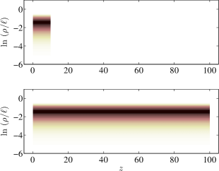
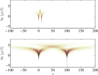
Figure 1: The natural log of $\rho^{2}\Delta^{2}(\rho,z)$ (integrand of (4) with $\,{\mathrm{d}}V_{\bm{\eta}}=2\pi\rho^{2}\,{\mathrm{d}}(\ln\rho)\,{\mathrm{d}}z$) for (a) a sphere of radius $\ell=1$ in inviscid flow, moving a path length $\lambda=10$ (top) and $100$ (bottom), plotted on the same scale. The scale of the integrand doesn’t change, only its support. Here $\bm{\eta}=(\rho,z)$ with $z$ the swimming direction and $\rho$ the distance from the $z$ axis. (b) Same as (a) but for a stresslet velocity field. The integral (4) grows linearly with $\lambda$ for both (a) and (b).

The second situation in which (4) shows diffusive behavior even for straight swimming paths is when the far-field velocity has the form of a stresslet, as is the case for a force-free swimmer in a viscous fluid. This diffusive behavior was observed in Lin et al. (2011) but it was Pushkin and Yeomans (2013) who provided a full explanation. For a stresslet swimmer, the main contributions to (4) come from $\lVert\bm{\eta}\rVert$ of order $\lambda$, so it is appropriate to use a point singularity model swimmer for large $\lambda$. In that case the drift function has the scaling $\Delta_{\lambda}(\bm{\eta})=\Delta_{\lambda}(\lambda\bm{\zeta})=\lambda^{-1}D(\bm{\zeta})$, where $\bm{\zeta}=\bm{\eta}/\lambda$ is a dimensionless variable and the function $D(\bm{\zeta})$ is independent of $\lambda$ for large $\lambda$ Pushkin and Yeomans (2013). Inserting this form in (4), we find

$$\int\Delta_{\lambda}^{2}(\bm{\eta})\,{\mathrm{d}}V_{\bm{\eta}}=\int\left(\lambda^{-2}D^{2}(\bm{\zeta})\right)\left(\lambda^{3}\,{\mathrm{d}}V_{\bm{\zeta}}\right)\sim\lambda.$$ (5)

The integral of $D^{2}(\bm{\zeta})$ converges despite having singularities Pushkin and Yeomans (2013). We thus see that the integral in (4) grows linearly in $\lambda$ for very different reasons than our first case: here the volume of particles affected by the swimmer grows as $\lambda^{3}$ (particles are affected further and further away), but they are displaced less (since they are further away, see Fig. 1). Any truncation of the integral in (5) (because of finite volume effect) will lead to a decrease in the diffusivity, a possible origin for the decrease in diffusivity with path length observed in Jepson et al. (2013). Note also that the reorientation mechanism discussed by Lin et al. (2011) is not necessary in this case to achieve the diffusive behavior, as pointed out by Pushkin and Yeomans (2014).

Having addressed the growth of the variance, we continue with finding the pdf of displacements for multiple swimmers. We write $X_{\lambda}^{N}$ for a single coordinate of $\bm{R}_{\lambda}^{N}$ (which coordinate is immaterial, because of isotropy). From (2) with $d=2$ we can compute $p_{X_{\lambda}^{1}}(x)$, the marginal distribution for one coordinate:

$$p_{X_{\lambda}^{1}}(x)=\int_{-\infty}^{\infty}p_{\bm{R}_{\lambda}^{1}}(\bm{r})\,{\mathrm{d}}y=\int_{V}\int_{-\infty}^{\infty}\frac{1}{2\pi r}\,\delta(r-\Delta_{\lambda}(\bm{\eta}))\,{\mathrm{d}}y\,\frac{\!\,{\mathrm{d}}V_{\bm{\eta}}}{V}.$$ (6)

Since $r^{2}=x^{2}+y^{2}$, the $\delta$-function will capture two values of $y$, and with the Jacobian included we obtain

$$p_{X_{\lambda}^{1}}(x)=\frac{1}{\pi}\int_{V}\frac{1}{\sqrt{\Delta_{\lambda}^{2}(\bm{\eta})-x^{2}}}\left[\Delta_{\lambda}(\bm{\eta})>\lvert x\rvert\right]\,\frac{\!\,{\mathrm{d}}V_{\bm{\eta}}}{V}\,,$$ (7)

where $\left[A\right]$ is an indicator function: it is $1$ if $A$ is satisfied, $0$ otherwise.

The marginal distribution in the three-dimensional case proceeds the same way from (2) with $d=3$:

$$p_{X_{\lambda}^{1}}(x)=\int_{-\infty}^{\infty}p_{\bm{R}_{\lambda}^{1}}(\bm{r})\,{\mathrm{d}}y\,{\mathrm{d}}z=\int_{V}\int_{-\infty}^{\infty}\int_{-\infty}^{\infty}\frac{1}{4\pi r^{2}}\,\delta(r-\Delta_{\lambda}(\bm{\eta}))\,{\mathrm{d}}y\,{\mathrm{d}}z\,\frac{\!\,{\mathrm{d}}V_{\bm{\eta}}}{V}.$$ (8)

Again with $r^{2}=x^{2}+y^{2}+z^{2}$ the $\delta$-function captures two values of $z$, and with the Jacobian included we obtain

$$p_{X_{\lambda}^{1}}(x)=\frac{1}{2\pi}\int_{V}\int_{-\infty}^{\infty}\frac{1}{\Delta_{\lambda}(\bm{\eta})}\,\frac{1}{\sqrt{\Delta_{\lambda}^{2}(\bm{\eta})-x^{2}-y^{2}}}\left[\Delta_{\lambda}^{2}(\bm{\eta})>x^{2}+y^{2}\right]\!\,{\mathrm{d}}y\,\frac{\!\,{\mathrm{d}}V_{\bm{\eta}}}{V}.$$ (9)

Now we integrate over $y$ to get

$$p_{X_{\lambda}^{1}}(x)=\tfrac{1}{2}\int_{V}\frac{1}{\Delta_{\lambda}(\bm{\eta})}\,\left[\Delta_{\lambda}(\bm{\eta})>\lvert x\rvert\right]\,\frac{\!\,{\mathrm{d}}V_{\bm{\eta}}}{V}$$ (10)

which is the three-dimensional analogue of (7). The integrand of (10) has an intuitive interpretation. The indicator function says that a displacement in a random direction must at least be larger than $\lvert x\rvert$ to project to a value $x$. The factor of $\Delta_{\lambda}(\bm{\eta})$ in the denominator then tells us that large displacements in a random direction are less likely to project to a value $x$. (The two-dimensional form (7) has essentially the same interpretation, with a different weight.)

In order to sum the displacements due to multiple swimmers, we need the characteristic function of $p_{X_{\lambda}^{1}}(x)$, defined by

$$\langle\mathrm{e}^{\mathrm{i}kX_{\lambda}^{1}}\rangle=\int_{-\infty}^{\infty}p_{X_{\lambda}^{1}}(x)\,\mathrm{e}^{\mathrm{i}kx}\,{\mathrm{d}}x.$$ (11)

For the two-dimensional pdf (7), we have

$$\langle\mathrm{e}^{\mathrm{i}kX_{\lambda}^{1}}\rangle=\int_{V}J_{0}(k\Delta_{\lambda}(\bm{\eta}))\,\frac{\!\,{\mathrm{d}}V_{\bm{\eta}}}{V}$$ (12)

where $J_{0}(x)$ is a Bessel function of the first kind. For the three-dimensional pdf (10), the characteristic function is

$$\langle\mathrm{e}^{\mathrm{i}kX_{\lambda}^{1}}\rangle=\int_{V}\operatorname{sinc}{(k\Delta_{\lambda}(\bm{\eta}))}\,\frac{\!\,{\mathrm{d}}V_{\bm{\eta}}}{V}$$ (13)

where $\operatorname{sinc}x\mathrel{\raisebox{0.29707pt}{:}\!\!=}x^{-1}\sin x$ for $x\neq 0$, and $\operatorname{sinc}0\mathrel{\raisebox{0.29707pt}{:}\!\!=}1$. The expression (13) appears in Pushkin and Yeomans (2014), except here we compute it directly from a spatial integral rather than from the pdf of $\Delta$. The main difference will come in the way we take the limit $V\rightarrow\infty$ below, which will allow us to study the number density dependence directly.

We define

$$\gamma(x)\mathrel{\raisebox{0.29707pt}{:}\!\!=}\begin{cases}1-J_{0}(x),\quad&d=2;\\ 1-\operatorname{sinc}x,\quad&d=3,\end{cases}$$ (14)

We have $\gamma(0)=\gamma^{\prime}(0)=0$, $\gamma^{\prime\prime}(0)=1/d$, so $\gamma(\xi)\sim(1/2d)\,\xi^{2}+\mathrm{O}(\xi^{4})$ as $\xi\rightarrow 0$. For large argument, $\gamma(\xi)\rightarrow 1$. We can then write the two cases (12)–(13) for the characteristic function together as

$$\langle\mathrm{e}^{\mathrm{i}kX_{\lambda}^{1}}\rangle=1-(v_{\lambda}/V)\,\Gamma_{\lambda}(k)$$ (15)

where

$$\Gamma_{\lambda}(k)\mathrel{\raisebox{0.29707pt}{:}\!\!=}\frac{1}{v_{\lambda}}\int_{V}\gamma(k\Delta_{\lambda}(\bm{\eta}))\,{\mathrm{d}}V_{\bm{\eta}}.$$ (16)

Here $v_{\lambda}$ is the volume ‘carved out’ by a swimmer moving a distance $\lambda$:

$$v_{\lambda}=\lambda\sigma$$ (17)

with $\sigma$ the cross-sectional area of the swimmer in the direction of motion.

Since we are summing independent particle displacements, the probability distribution of the sum is the convolution of $N$ one-swimmer distributions. Using the Fourier transform convolution property, the characteristic function for $N$ swimmers is thus $\langle\mathrm{e}^{\mathrm{i}kX_{\lambda}^{N}}\rangle=\langle\mathrm{e}^{\mathrm{i}kX_{\lambda}^{1}}\rangle^{N}$. From (15),

$$\langle\mathrm{e}^{\mathrm{i}kX_{\lambda}^{1}}\rangle^{N}=\left(1-v_{\lambda}\Gamma_{\lambda}(k)/V\right)^{nV},$$ (18)

where we used $N=nV$, with $n$ the number density of swimmers. We will need the following simple result:

Proposition 1.

Let $y(\varepsilon)\sim\mathrm{o}(\varepsilon^{-M/(M+1)})$ as $\varepsilon\rightarrow 0$ for an integer $M\geq 1$; then

$$(1-\varepsilon y(\varepsilon))^{1/\varepsilon}=\exp\biggl{(}-\sum_{m=1}^{M}\frac{\varepsilon^{m-1}y^{m}(\varepsilon)}{m}\biggr{)}\left(1+\mathrm{o}(\varepsilon^{0})\right),\quad\varepsilon\rightarrow 0.$$ (19)

See Appendix A for a short proof.

Let’s examine the assumption of Proposition 1 for $M=1$ applied to (18), with $\varepsilon=1/V$ and $y=v_{\lambda}\Gamma_{\lambda}(k)$. For $M=1$, the assumption of Proposition 1 requires

$$\Gamma_{\lambda}(k)\sim\mathrm{o}(V^{1/2}),\qquad V\rightarrow\infty.$$ (20)

A stronger divergence with $V$ means using a larger $M$ in Proposition 1, but we shall not need to consider this here. Note that it is not possible for $\Gamma_{\lambda}(k)$ to diverge faster than $\mathrm{O}(V)$, since $\gamma(x)$ is bounded. In order for $\Gamma_{\lambda}(k)$ to diverge as $\mathrm{O}(V)$, the displacement must be nonzero as $V\rightarrow\infty$, an unlikely situation that can be ruled out.

Assuming that (20) is satisfied, we use Proposition 1 with $M=1$ to make the large-volume approximation

$$\langle\mathrm{e}^{\mathrm{i}kX_{\lambda}^{1}}\rangle^{N}=\left(1-v_{\lambda}\Gamma_{\lambda}(k)/V\right)^{nV}\sim\exp\left(-nv_{\lambda}\,\Gamma_{\lambda}(k)\right),\quad V\rightarrow\infty.$$ (21)

If the integral $\Gamma_{\lambda}(k)$ is convergent as $V\rightarrow\infty$ we have achieved a volume-independent form for the characteristic function, and hence for the distribution of $x$ for a fixed swimmer density. We define the quantity

$$\nu_{\lambda}\mathrel{\raisebox{0.29707pt}{:}\!\!=}nv_{\lambda}=\lambda/\ell_{\text{mfp}}$$ (22)

where $\ell_{\text{mfp}}=(n\sigma)^{-1}$ is the swimmer mean free path. Since $v_{\lambda}$ is the volume carved out by a single swimmer moving a distance $\lambda$ (Eq. (17)), $\nu_{\lambda}$ is the expected number of swimmers that will ‘hit’ a given fluid particle.

A comment is in order about evaluating (16) numerically: if we take $\lvert k\rvert$ to $\infty$, then $\gamma(k\Delta)\rightarrow 1$, and thus $v_{\lambda}\Gamma\rightarrow V$, which then leads to $\mathrm{e}^{-N}$ in (21). This is negligible as long as the number of swimmers $N$ is moderately large. In practice, this means that $\lvert k\rvert$ only needs to be large enough that the argument of the decaying exponential in (21) is of order one, that is

$$\nu_{\lambda}\,\Gamma_{\lambda}(k_{\text{max}})\sim\mathrm{O}(1).$$ (23)

Wavenumbers $\lvert k\rvert>k_{\text{max}}$ do not contribute to (21). (We are assuming monotonicity of $\Gamma_{\lambda}(k)$ for $k>0$, which will hold for our case.) Note that (23) implies that we need larger wavenumbers for smaller densities $n$: a typical fluid particle then encounters very few swimmers, and the distribution should be far from Gaussian.

Now that we’ve computed the characteristic function for $N$ swimmers (21), we finally recover the pdf of $x$ for $N=nV$ swimmers as the inverse Fourier transform

$$p_{X_{\lambda}}(x)=\frac{1}{2\pi}\int_{-\infty}^{\infty}\exp\left(-\nu_{\lambda}\,\Gamma_{\lambda}(k)\right)\mathrm{e}^{-\mathrm{i}kx}\,{\mathrm{d}}k,$$ (24)

where we dropped the superscript $N$ from $X_{\lambda}^{N}$ since the number of swimmers no longer enters the expression directly.

III Comparing to experiments

We now compare the theory discussed in the previous sections to the experiments of Leptos et al.  in particular the observed dependence of the distribution on the number density $\phi$. (Another aspect of their experiments, the ‘diffusive scaling’ of the distributions, will be discussed in Section VI.) In their experiments they use the microorganism C. reinhardtii, an alga of the ‘puller’ type, since its two flagella are frontal. This organism has a roughly spherical body with radius $\ell\approx 5\,\mu\mathrm{m}$. They observe a distribution of swimming speeds with a strong peak around $100\,\mu\mathrm{m}/\mathrm{s}$. They place fluorescent microspheres of about a micron in radius in the fluid, and optically measure their displacement as the organisms move. The volume fraction of organisms varies from $\phi=0\%$ (pure fluid) to $2.2\%$.

They measure the displacement of the microspheres along a reference direction, arbitrarily called $x$ (the system is assumed isotropic). Observing many microspheres allows them to compute the pdf of tracer displacements $X_{\lambda}$, which we’ve denoted $p_{X_{\lambda}}(x)$. Thus, $p_{X_{\lambda}}(x)\,{\mathrm{d}}x$ is the probability of observing a particle displacement $X_{\lambda}\in[x,x+\,{\mathrm{d}}x]$ after a path length $\lambda$. (They write their density $P(\Delta x,\Delta t)$, where $(\Delta x,\Delta t)$ are the same as our $(x,\lambda/U)$.)

At zero volume fraction ($\phi=0$), the pdf $p_{X_{\lambda}}(x)$ is Gaussian, due solely to thermal noise. For higher number densities, Leptos et al. see exponential tails appear and the Gaussian core broaden. The distribution is well-fitted by the sum of a Gaussian and an exponential:

$$p_{X_{\lambda}}(x)=\frac{1-f}{\sqrt{2\pi\delta_{\text{g}}^{2}}}\,\mathrm{e}^{-x^{2}/2\delta_{\text{g}}^{2}}+\frac{f}{2\delta_{\text{e}}}\,\mathrm{e}^{-\lvert x\rvert/\delta_{\text{e}}}.$$ (25)

They observe the scalings $\delta_{\text{g}}\approx A_{\text{g}}t^{1/2}$ and $\delta_{\text{e}}\approx A_{\text{e}}t^{1/2}$, where $A_{\text{g}}$ and $A_{\text{e}}$ depend on $\phi$. The dependence on $t^{1/2}$ is referred to as the ‘diffusive scaling’ and will be discussed in Section VI. Exploiting this scaling, Eckhardt and Zammert (2012) have fitted these distributions very well to a continuous-time random walk model, but this does not suggest a mechanism.

We shall use a model swimmer of the squirmer type Lighthill (1952); Blake (1971); Ishikawa et al. (2006); Ishikawa and Pedley (2007); Drescher et al. (2009), with axisymmetric streamfunction Lin et al. (2011)

$$\Psi_{\text{sf}}(\rho,z)=\tfrac{1}{2}{\rho^{2}\,U}\left\{-1+\frac{\ell^{3}}{(\rho^{2}+z^{2})^{3/2}}+\tfrac{3}{2}\frac{\beta\ell^{2}z}{(\rho^{2}+z^{2})^{3/2}}\left(\frac{\ell^{2}}{\rho^{2}+z^{2}}-1\right)\right\}$$ (26)

in a frame moving at speed $U$. Here $z$ is the swimming direction and $\rho$ is the distance from the $z$ axis. To mimic C. reinhardtii, we use $\ell=5\,\mu\mathrm{m}$ and $U=100\,\mu\mathrm{m}/\mathrm{s}$. (Leptos et al. (2009) observe a distribution of velocities but the peak is near $100\,\mu\mathrm{m}/\mathrm{s}$.) We take $\beta=0.5$ for the relative stresslet strength, which gives a swimmer of the puller type, just like C. reinhardtii. The contour lines of the axisymmetric streamfunction (26) are depicted in Fig. 2. The parameter $\beta=0.5$ is the only one that was fitted (visually) to give good agreement later.

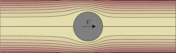
Figure 2: Contour lines for the axisymmetric streamfunction of a squirmer of the form (26), with $\beta=0.5$. This swimmer is of the puller type, as for C. reinhardtii.

First we compute the drift function $\Delta_{\lambda}(\bm{\eta})$ for a single swimmer moving along the $z$ axis. The model swimmer is axially symmetric, so $\bm{\eta}$ can be written in terms of $z$ and $\rho$, the perpendicular distance to the swimming axis. We take $\lambda=12\,\mu\mathrm{m}$, since the time is $t=0.12\,\mathrm{s}$ in Fig. 2(a) of Leptos et al., and our swimmer moves at speed $U=100\,\mu\mathrm{m}/\mathrm{s}$. We compute $\Delta_{\lambda}(\rho,z)$ for a large grid of $\ln\rho$ and $z$ values, using the analytic far-field stresslet form for the displacement Dunkel et al. (2010); Miño et al. (2013); Pushkin and Yeomans (2013) when far away from the swimmer’s path.

From the drift function $\Delta_{\lambda}(\bm{\eta})$ we now want to compute $\Gamma_{\lambda}(k)$ defined by (16). To estimate how large a $k$ value we will need, we start from the smallest volume fraction in the experiments, $\phi\sim 0.4\%$. For spherical swimmers of radius $\ell\sim 5\,\mu\mathrm{m}$ (with cross-sectional area $\sigma=\pi\ell^{2}\sim 78.5\,\mu\mathrm{m}^{2}$), this gives a number density of $7.6\times 10^{-6}\,\mu\mathrm{m}^{-3}$. We thus get $\nu_{\lambda}=n\sigma\lambda\sim 7.2\times 10^{-3}$. The criterion (23) then tells us that we need $k_{\text{max}}$ large enough that $\Gamma_{\lambda}(k_{\text{max}})\sim 1/\nu_{\lambda}\sim 139$.

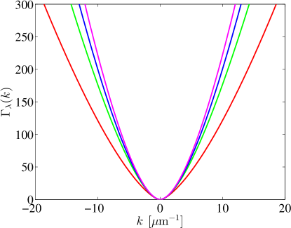
Figure 3: The function $\Gamma_{\lambda}(k)$ defined by Eq. (16) for (from broadest to narrowest) $\lambda=12\,\mu\mathrm{m}$, $36\,\mu\mathrm{m}$, $60\,\mu\mathrm{m}$, and $96\,\mu\mathrm{m}$.

Figure 3 shows the numerically-computed $\Gamma_{\lambda}(k)$ for several values of $\lambda$, with $\lambda=12\,\mu\mathrm{m}$ the broadest curve. We can see from the figure that choosing $k_{\text{max}}\sim 20\,\mu\mathrm{m}^{-1}$ will ensure that $\nu_{\lambda}\Gamma_{\lambda}(k_{\text{max}})$ is large enough. As $\lambda$ gets larger, $k_{\text{max}}$ decreases, reflecting the trend towards the central limit theorem (which corresponds to the small-$k$ expansion of $\Gamma_{\lambda}(k)$, see Section V). Note also that $\Gamma_{\lambda}(k)$ tends to become independent of $\lambda$ as $\lambda$ gets larger.

To obtain $p_{X_{\lambda}}(x)$ and compare to Leptos et al., we must now take the inverse Fourier transform of $\exp(-\nu_{\lambda}\Gamma_{\lambda}(k))$, as dictated by (24). This is straightforward using Matlab’s ifft routine. The ‘period’ (domain in $x$) is controlled by the spacing of the $k$ grid, so we make sure the grid is fine enough to give us the largest values of $x$ required. We also convolve with a Gaussian distribution of half-width $\sqrt{2D_{0}t}=0.26\,\mu\mathrm{m}$ to mimic thermal noise. This follows from the value $D_{0}=0.28\,\mu\mathrm{m}^{2}/\mathrm{s}$ measured by Leptos et al. for the diffusivity of the microspheres. The value of $D_{0}$ is consistent with the Stokes–Einstein equation for the diffusivity of thermally-agitated small spheres in a fluid.

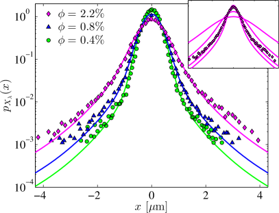
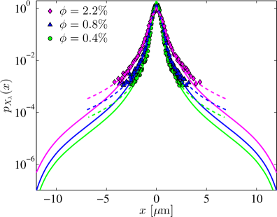
Figure 4: (a) The pdf of particle displacements after a path length $\lambda=12\,\mu\mathrm{m}$, for several values of the volume fraction $\phi$. The data is from Leptos et al. (2009), and the figure should be compared to their Fig. 2(a). The theoretical curves were obtained from (24) for the model squirmer in Fig. 2, with some noise corresponding to thermal diffusivity as measured in Leptos et al. (2009). Inset: comparison of (from broadest to narrowest) $\beta=2$, $1$, $0.5$, and $0.1$, for $\phi=2.2\%$, showing the sensitivity of the fit $\beta=0.5$. (b) Same as (a) but on a wider scale, also showing the form suggested by Eckhardt and Zammert (2012) (dashed lines).

The results are plotted in Fig. 4 and compared to the data of Fig. 2(a) of Leptos et al. (2009). The agreement is excellent: we remind the reader that we adjusted only one parameter, $\beta=0.5$. This parameter was visually adjusted to the $\phi=2.2\%$ data in Fig. 4, since the larger concentration is most sensitive to $\beta$; a more careful fit is unnecessary given the uncertainties in both model and data. (The inset shows the sensitivity of the fit to $\beta$.) All the other physical quantities were gleaned from Leptos et al.  What is most remarkable about the agreement in Fig. 4 is that it was obtained using a model swimmer, the spherical squirmer, which is not expected to be such a good model for C. reinhardtii. The real organisms are strongly time-dependent, for instance, and do not move in a perfect straight line. Nevertheless the model captures very well the pdf of displacements, in particular the volume fraction dependence. The model swimmer slightly underpredicts the tails, but since the tails are associated to large displacements they depend on the near-field details of the swimmer, so it is not surprising that our model swimmer should deviate from the data.

In Figure 4 we compare our results to the phenomenological fit of Eckhardt and Zammert (2012) based on continuous-time random walks: their fit is better in the tails, but our models disagree immediately after the data runs out. Our model has the realistic feature that the distribution is cut off at the path length $\lambda=12\,\mu\mathrm{m}$, since it is extremely unlikely that a particle had two close encounters with a swimmer at these low volume fractions.

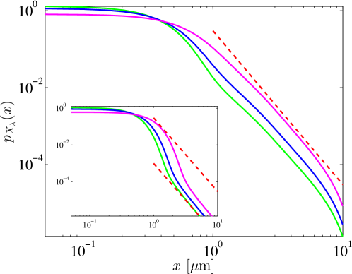
Figure 5: The same distributions as in Fig. 4, but on a log-log plot. The dashed line is the $x^{-4}$ power law predicted by Pushkin and Yeomans (2014). Inset: numerical simulation with only the stresslet far-field displacement included.

A possible explanation as to why the squirmer model does so well was provided by Pushkin and Yeomans (2014). They used numerical simulations of squirmers (with a larger value $\beta=2$ that leads to a trapped volume) to show that the tails of distribution scale as $x^{-4}$, which is the asymptotic form of the stresslet displacement distribution. Figure 5 shows that our computations have a similar tail, though we emphasize here that our agreement with the experiments of Leptos et al. (2009) is quantitative and correctly reproduces the volume fraction dependence. We also point out that though the trend in Fig. 5 follows $x^{-4}$, the slope changes gradually and does not have a clear power law (the log scale means the deviations are quite large). The inset in Fig. 5 is a numerical simulation that includes only the singularity in the stresslet displacement, $\Delta(\bm{\eta})\sim\lVert\bm{\eta}\rVert^{-1}$, as assumed in the analysis of Pushkin and Yeomans (2014). Though the $x^{-4}$ tails are eventually achieved, they have far lower probability than needed to explain the numerics. Pushkin and Yeomans’s use of the far-field stresslet form to predict the tails is thus questionable, at least for short path lengths.

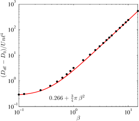
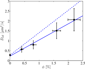
Figure 6: (a) For the squirmer model (26), dependence of the effective diffusivity $D_{\text{eff}}$ on the stresslet strength $\beta$. For small $\beta$, we recover the value for spheres in inviscid flow Thiffeault and Childress (2010). An approximate formula is also shown as a solid curve. (b) Comparison of the effective diffusivity data from Leptos et al. (2009), showing their fit (solid line). The dashed line is the prediction for $\beta=0.5$, used in this paper.

For the effective diffusivity, Leptos et al. (2009) give the formula $D_{\text{eff}}\simeq D_{0}+\alpha\,\phi$, with $D_{0}=0.23\,\mu\mathrm{m}/\mathrm{s}^{2}$ and $\alpha=81.3\,\mu\mathrm{m}/\mathrm{s}^{2}$. Elsewhere in their paper they also give $D_{0}=0.28\,\mu\mathrm{m}/\mathrm{s}^{2}$ for the diffusivity of the microspheres in the absence of swimmers, but their fitting procedure changes the intercept slightly. (Here we used $D_{0}=0.28\,\mu\mathrm{m}/\mathrm{s}^{2}$, but the difference is minute.) Figure 6 shows the numerically-computed effective diffusivity for our squirmer model, as a function of $\beta$. This curve is as in Lin et al. (2011), Fig. 6(a), except that we corrected the integrals in the far field using the analytic expression of Pushkin and Yeomans (2013), which gives a more accurate result. The Figure also shows the fit

$$\frac{D_{\text{eff}}-D_{0}}{Un\ell^{4}}\simeq 0.266+\tfrac{3}{4}\pi\beta^{2},$$ (27)

which is fairly good over the whole range (keeping in mind that this is a logarithmic plot, so the discrepancy at moderate $\beta$ are of the order of $20$–$30\%$). Here the value $0.266$ is the diffusivity due to spheres in inviscid flow ($\beta=0$, see Thiffeault and Childress (2010)), and $\tfrac{3}{4}\pi\beta^{2}$ is the large-$\beta$ analytic expression Pushkin and Yeomans (2013) for stresslets. From the data in Fig. 6 we find $\alpha\simeq 113\,\mu\mathrm{m}/\mathrm{s}^{2}$, significantly larger than Leptos et al. (2009), as can be seen in Fig. 6. The solid line is their fit, the dashed is our model prediction for $\beta=0.5$. The overestimate is likely due to the method of fitting to the squared displacement: their Fig. 3(a) clearly shows a change in slope with time, and the early times tend to be steeper, which would increase the effective diffusivity. Note also that their Fig. 3(a) has a much longer temporal range than their PDFs, going all the way to $2\,\mathrm{s}$ (compared to $0.3\,\mathrm{s}$), raising the possibility that particles were lost by moving out of the focal plane.

IV The ‘interaction’ viewpoint

Equation (24) gives the exact solution for the distribution of uncorrelated displacements due to swimmers of number density $n$. In this section we derive an alternative form, in terms of an infinite series, which is often useful and provides an elegant interpretation for (24).

The displacement $\Delta_{\lambda}(\bm{\eta})$ typically decays rapidly away from the swimmer, so that it may often be taken to vanish outside a specified ‘interaction volume’ $\widetilde{V}_{\lambda}$. Then from (16), since $\gamma(0)=0$, we have

$$\Gamma_{\lambda}(k)=\frac{1}{v_{\lambda}}\int_{\widetilde{V}_{\lambda}}\gamma(k\Delta_{\lambda}(\bm{\eta}))\,{\mathrm{d}}V_{\bm{\eta}}\\ =\frac{\widetilde{V}_{\lambda}}{v_{\lambda}}\left(1-\widetilde{\Gamma}_{\lambda}(k)\right)$$ (28)

where

$$\widetilde{\Gamma}_{\lambda}(k)=\frac{1}{\widetilde{V}_{\lambda}}\int_{\widetilde{V}_{\lambda}}(1-\gamma(k\Delta_{\lambda}(\bm{\eta})))\,{\mathrm{d}}V_{\bm{\eta}}\,.$$ (29)

Define $\tilde{\nu}_{\lambda}\mathrel{\raisebox{0.29707pt}{:}\!\!=}n\widetilde{V}_{\lambda}$; we insert (28) into (24) and Taylor expand the exponential to obtain

$$p_{X_{\lambda}}(x)=\sum_{m=0}^{\infty}\frac{\tilde{\nu}_{\lambda}^{m}}{m!}\,\mathrm{e}^{-\tilde{\nu}_{\lambda}}\,\frac{1}{2\pi}\int_{-\infty}^{\infty}\widetilde{\Gamma}_{\lambda}^{m}(k)\,\mathrm{e}^{-\mathrm{i}kx}\,{\mathrm{d}}k.$$ (30)

The factor $\tilde{\nu}_{\lambda}^{m}\,\mathrm{e}^{-\tilde{\nu}_{\lambda}}/m!$ is a Poisson distribution for the number of ‘interactions’ $m$ between swimmers and a particle: it measures the probability of finding $m$ swimmers inside the volume $\widetilde{V}_{\lambda}$. The inverse transform in (30) gives the $m$-fold convolution of the single-swimmer displacement pdf. This was the basis for the model used in Thiffeault and Childress (2010); Lin et al. (2011) and in an earlier version of this paper Thiffeault (2014). We have thus shown that formula (24) is the natural infinite-volume limit of the interaction picture.

Formula (30) is very useful in many instances, such as when $\tilde{\nu}_{\lambda}$ is small, in which case only a few terms are needed in (30) for a very accurate representation. Note that the first term of the sum in (30) is a $\delta$-function, which corresponds to particles that are outside the interaction volume $\widetilde{V}_{\lambda}$. This singular behavior disappears after $p_{X_{\lambda}}(x)$ is convolved with a Gaussian distribution associated with molecular noise.

Let us apply (30) to a specific example. A model for cylinders and spheres of radius $\ell$ traveling along the $z$ axis in an inviscid fluid Thiffeault and Childress (2010); Lin et al. (2011) is the log model,

$$\Delta_{\lambda}(\bm{\eta})=\begin{cases}C\ln^{+}(\ell/\rho),&\text{if $0\leq z\leq\lambda$,}\\ 0,&\text{otherwise},\end{cases}$$ (31)

where $\rho$ is the perpendicular distance to the swimming direction and $\ln^{+}x\mathrel{\raisebox{0.29707pt}{:}\!\!=}\ln\max(x,1)$. The logarithmic form comes from the stagnation points on the surface of the swimmer, which dominate transport in this inviscid limit. This model is also appropriate for a spherical ‘treadmiller’ swimmer in viscous flow. The drift function (31) resembles Fig. 1.

For the form (31) the interaction volume $\widetilde{V}_{\lambda}$ is the same as $v_{\lambda}$, the volume carved out during the swimmer’s motion (Eq. (17)). By changing integration variable from $\rho$ to $\Delta$ in (16) we can carry out the integrals explicitly to obtain (see Appendix B)

$$\widetilde{\Gamma}_{\lambda}(k)=\begin{cases}(1+(Ck)^{2})^{-1/2},\qquad&\text{(cylinders)};\\ (Ck/2)^{-1}\arctan(Ck/2),\qquad&\text{(spheres)}.\end{cases}$$ (32)

This is independent of $\lambda$, even for short paths (but note that (31) is not a good model for $\lambda<\ell$).

Furthermore, for $d=2$ we can also explicitly obtain the convolutions that arise in (30) to find the full distribution,

$$p_{X_{\lambda}}(x)=\mathrm{e}^{-\nu_{\lambda}}\left(\delta(x)+\sum_{m=1}^{\infty}\frac{\nu_{\lambda}^{m}}{m!}\,\frac{1}{C\sqrt{\pi}\,\Gamma(m/2)}\left(\lvert x\rvert/2C\right)^{(m-1)/2}K_{(m-1)/2}(\lvert x\rvert/C)\right),$$ (33)

where $K_{\alpha}(x)$ are modified Bessel functions of the second kind, and $\Gamma(x)$ is the Gamma function (not to be confused with $\Gamma_{\lambda}(k)$ above). Equation (33) is a very good approximation to the distribution of displacements due to inviscid cylinders. Unfortunately no exact form is known for spheres: we must numerically evaluate (24) with (32) or use asymptotic methods (see Section V).

V Long paths: Large-deviation theory

In Section IV we derived an alternative form of our master equation (24) as an expansion in an ‘interaction’ volume. Here we look at another way to evaluate the inverse Fourier transform in (24), using large-deviation theory Gärtner (1977); Ellis (1984, 1985); Touchette (2009). In essence, large-deviation theory is valid in the limit when a particle encounters many swimmers, so that $\nu_{\lambda}$ is large (in practice ‘large’ often means order one for a reasonable approximation). This includes the central limit theorem (Gaussian form) as a special case. In this section we provide a criterion for how much time is needed before Gaussian behavior is observed, which can help guide future experiments.

Earlier we used the characteristic function (21). Here it is more convenient to work with the moment-generating function, which in our case can be obtained simply by letting $s=\mathrm{i}k$. The moment-generating function of the distribution is then

$$\langle\mathrm{e}^{sX_{\lambda}}\rangle=\exp\left(-\nu_{\lambda}\,\Gamma_{\lambda}(-\mathrm{i}s)\right)=\exp\left(\nu_{\lambda}\,\Lambda(s)\right)$$

where $\nu_{\lambda}$ was defined by Eq. (22), and

$$\Lambda(s)\mathrel{\raisebox{0.29707pt}{:}\!\!=}\frac{1}{\nu_{\lambda}}\ln\langle\mathrm{e}^{sX_{\lambda}}\rangle=-\Gamma_{\lambda}(-\mathrm{i}s)$$ (34)

is the scaled cumulant-generating function. As its name implies, this function has the property that its derivatives at $s=0$ give the cumulants of $X_{\lambda}$ scaled by $\nu_{\lambda}$, for example

$$\Lambda^{\prime\prime}(0)=\nu_{\lambda}^{-1}\langle X_{\lambda}^{2}\rangle,\qquad\Lambda^{\prime\prime\prime\prime}(0)=\nu_{\lambda}^{-1}\left(\langle X_{\lambda}^{4}\rangle-3\langle X_{\lambda}^{2}\rangle^{2}\right),$$ (35)

where we left out the vanishing odd moments. We left out the $\lambda$ subscript on $\Lambda(s)$ since we assume that it becomes independent of $\lambda$ for large $\lambda$.

If $\Lambda(s)$ is differentiable over some interval of interest, $p_{X_{\lambda}}(x)$ satisfies a large-deviation principle Gärtner (1977); Ellis (1984, 1985); Touchette (2009),

$$p_{X_{\lambda}}(x)\sim\mathrm{e}^{-\nu_{\lambda}\,I(x/\nu_{\lambda})+\mathrm{o}(\nu_{\lambda})},\qquad\nu_{\lambda}\gg 1,$$ (36)

where $I(X)$ is the rate function, which is the Legendre–Fenchel transformation of $\Lambda(s)$:

$$I(X)=\sup_{s\in\mathbb{R}}\{sX-\Lambda(s)\}.$$ (37)

The large-deviation principle is in essence an application of the method of steepest descent for large $\nu_{\lambda}$.

The scaled cumulant-generating function $\Lambda(s)$ is always convex, which guarantees a unique solution to (37). The rate function $I(X)$ is also convex, with a global minimum at $X=0$. This means that for small $X=x/\nu_{\lambda}$ we can use the Taylor expansion

$$I(X)=\tfrac{1}{2}I^{\prime\prime}(0)X^{2}+\tfrac{1}{4!}I^{\prime\prime\prime\prime}(0)X^{4}+\mathrm{O}(X^{6})$$ (38)

to write

$$p_{X_{\lambda}}(x)\sim\mathrm{e}^{-\tfrac{1}{2}I^{\prime\prime}(0)\,x^{2}/\nu_{\lambda}},\qquad x\ll c\,\nu_{\lambda},\quad\nu_{\lambda}\gg 1,$$ (39)

with $c=\lvert 12I^{\prime\prime}(0)/I^{\prime\prime\prime\prime}(0)\rvert^{1/2}$. This is a Gaussian approximation with variance $\nu_{\lambda}/I^{\prime\prime}(0)$, which can be shown to agree with (4) after multiplying by $d$. To recover a Gaussian distribution over an appreciable range of $x$ (say, a standard deviation) we insert $x\sim\sqrt{\nu_{\lambda}/I^{\prime\prime}(0)}$ in the condition $x\ll c\,\nu_{\lambda}$ to find the Gaussian criterion

$$\nu_{\lambda}\gg\frac{1}{12}\,\frac{\lvert I^{\prime\prime\prime\prime}(0)\rvert}{(I^{\prime\prime}(0))^{2}}=\frac{1}{12}\,\frac{\lvert\Lambda^{\prime\prime\prime\prime}(0)\rvert}{(\Lambda^{\prime\prime}(0))^{2}}.$$ (40)

After using $\Lambda(s)$ to find the cumulants, we can rewrite this as

$$\Phi_{\lambda}\mathrel{\raisebox{0.29707pt}{:}\!\!=}\frac{(d+3)}{40}\,\frac{v_{\text{sw}}\int_{V}\Delta_{\lambda}^{4}(\bm{\eta})\,{\mathrm{d}}V_{\bm{\eta}}}{\left(\int_{V}\Delta_{\lambda}^{2}(\bm{\eta})\,{\mathrm{d}}V_{\bm{\eta}}\right)^{2}}\ll\phi,$$ (41)

where $v_{\text{sw}}$ is the volume of one swimmer. When (40) or (41) is satisfied, we can expect that the distribution will be Gaussian (except in the far tails). (The constant prefactor in (41) is only valid for $d=2$ or $3$.) The criterion (41) can be interpreted as the minimum volume fraction $\Phi_{\lambda}$ required to observe Gaussian behavior, roughly within a standard deviation of the mean. We note that, at small swimmer volume fraction, a long time (i.e., path length $\lambda$) is required to achieve the Gaussian form. Figure 7 highlights this: the solid curve is $\Phi_{\lambda}$ from Eq. (41) for the squirmer model in Section III, with parameter values appropriate for the experiments of Leptos et al. (2009). Their experiments had $\lambda\lesssim 30\,\mu\mathrm{m}$, so they are in the slowly-decreasing region of Fig. 7, before more rapid $\lambda^{-1}$ convergence sets in after $\lambda\gtrsim 50\,\mu\mathrm{m}$. It is thus not surprising that Gaussian tails were not observed in the experiments.

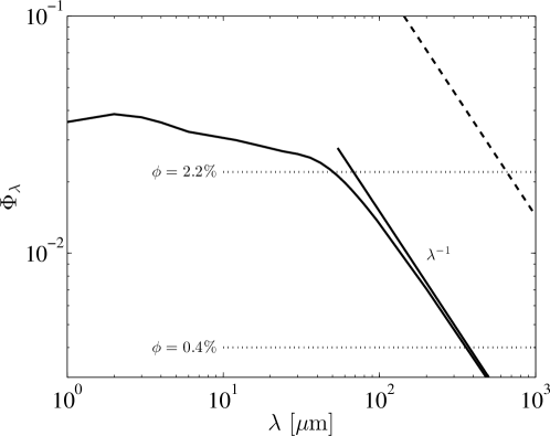
Figure 7: The minimum volume fraction $\Phi_{\lambda}$ for the threshold of Gaussian behavior (Eq. (41)). The solid line is the the squirmer model (Section III) with $\beta=0.5$ and radius $\ell=5\,\mu\mathrm{m}$. The dashed line is for spherical treadmillers (inviscid spheres) of the same radius. The latter require an order of magnitude longer to achieve Gaussianity, due to the short range of their velocity field.

As an illustration of the large-deviation approach, we consider again the inviscid cylinder and sphere results (32). We have then respectively

$$\Lambda(s)=\begin{cases}(1-(Cs)^{2})^{-1/2}-1,\qquad&\text{(cylinders)};\\ (Cs/2)^{-1}\operatorname{arctanh}(Cs/2)-1,\qquad&\text{(spheres)}.\end{cases}$$ (42)

We can see from (37) that the singularities in (42) ($\lvert s\rvert=1/C$ for cylinders, $\lvert s\rvert=2/C$ for spheres) immediately lead to $I(X)\sim\lvert X\rvert/C$ and $2\lvert X\rvert/C$ as $\lvert X\rvert\rightarrow\infty$, respectively, corresponding to exponential tails in (36) independent of $\nu_{\lambda}$. These are the displacements of particles that come near the stagnation points at the surface of the cylinder or sphere Lin et al. (2011). We can also use (42) to compute the constant on the right-hand side of (40): $3/4$ (cylinders) and $9/10$ (spheres), which are both of order unity. This reflects the fact that the drift function $\Delta_{\lambda}(\bm{\eta})$ is very localized, so convergence to Gaussian is tied directly to the volume carved out by the swimmers. For swimmers with a longer-range velocity field, such as squirmers, the constant is much larger, as reflected by the large difference between the solid (squirmers) and the dashed (inviscid spheres) curves in Fig. 7.

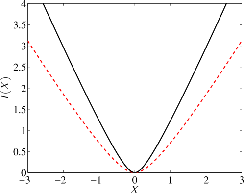
Figure 8: The rate function $I(X)$ for cylinders (Eq. (43), dashed line) and spheres (solid line, numerical solution of (36)). In both cases we used $C=1$. The linear behavior for large $\lvert X\rvert$ indicates exponential tails in (36). When $X$ is small, expanding near the quadratic minimum recovers the Gaussian limit.

For inviscid cylinders the Legendre–Fenchel transform (37) can be done explicitly to find (with $C=1$)

$$I(X)=1-\sqrt{3\pi\alpha}\left(12-\alpha^{2}X^{-2}\right)^{-1/2}+\tfrac{1}{2}\sqrt{\pi\alpha}\left(\left(\pi\alpha-4\right)\alpha^{-2}X^{2}+\tfrac{1}{3}\right)^{1/2}$$ (43)

where $\alpha(X)\geq 0$ is defined by

$$\alpha^{3}(X)=6\left(\sqrt{(9\pi X^{4})^{2}+48X^{6}}-9\pi X^{4}\right).$$ (44)

For spheres (37) must be solved numerically for each $X$, which is straightforward since this is a one-dimensional problem with a unique solution. The function $I(X)$ for both cylinders and spheres is plotted in Fig. 8.

VI The diffusive scaling

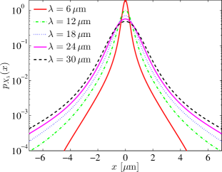
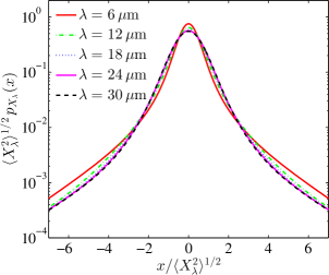
Figure 9: (a) pdfs of particle displacements for squirmers for different times, at a number density $\phi=2.2\%$. (b) The same pdfs rescaled by their standard deviation exhibit the ‘diffusive scaling’ observed in the experiments of Leptos et al. (2009), where the curves collapse onto one despite not being Gaussian. As in the experiments, the scaling is worst for $\lambda=6\,\mu\mathrm{m}$.

One of the most remarkable property of the pdfs found by Leptos et al. is the diffusive scaling. This is illustrated in Fig. 9: the unrescaled displacement pdfs are shown in Fig. 9; the same pdfs are shown again in Fig. 9, but rescaled by their standard deviation. The pdfs collapse onto a single curve (the shortest path length collapses more poorly). Figure 9 was obtained in the same manner as Fig. 4, using our probabilistic approach. Hence, the diffusive scaling is also present in our model, as it was in the direct simulations of Lin et al. (2011) for a similar range of path lengths. In Fig. 9 we left out thermal diffusion completely, which shows that it is not needed for the diffusive scaling to emerge.

Here we have the luxury of going much further in time and to examine the probability of larger displacements, since we are simply carrying out integrals and not running a statistically-limited experiment or simulation. (The numerical integrals are of course limited by resolution.) Figure 10 shows much longer runs (maximum $\lambda=500\,\mu\mathrm{m}$ compared to $30\,\mu\mathrm{m}$ in the experiments). We see that, though the diffusive scaling holds in the core (as it must, since the core is Gaussian), the tails are narrowing, consistent with convergence to a Gaussian distribution but breaking the diffusive scaling. We now explain why the diffusive scaling appears to hold for some time, but eventually breaks down.

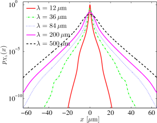
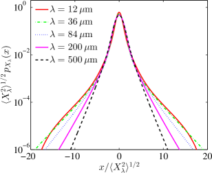
Figure 10: Same as Fig. 9 but for longer times and with a wider scale. In (a) the distributions broaden with time since their standard deviation is increasing; in (b), after rescaling by the standard deviation, the distributions’ tails narrow with increasing $\lambda$ as they converge to a Gaussian.

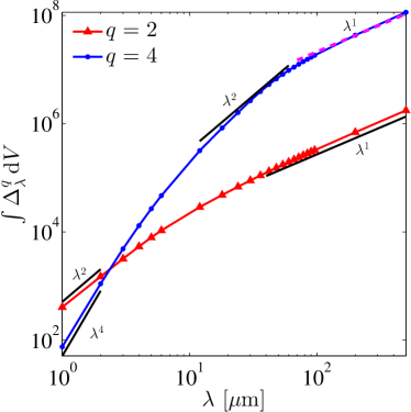
Figure 11: The second and fourth integrated moments of $\Delta_{\lambda}$. These grow ballistically ($\lambda^{q}$) for short times, and eventually grow linearly with $\lambda$. The slow crossover of $\Delta_{\lambda}^{4}$ is the origin of the ‘diffusive scaling’ of Leptos et al. (2009), since in their narrow range of $\lambda$ the curve is tangent to $\lambda^{2}$.

To understand the origin of the diffusive scaling, let us first examine how the integrated moments of $\Delta_{\lambda}$ change with $\lambda$. Figure 11 shows the evolution of the spatial integrals of $\Delta_{\lambda}^{2}$ and $\Delta_{\lambda}^{4}$ for our squirmer model. For short $\lambda$, the moment of $\Delta_{\lambda}^{q}$ grows as $\lambda^{q}$. This is a typical ‘ballistic’ regime: it occurs because for short times the integrals are dominated by fluid particles that are displaced proportionately to the swimmer’s path length. These particles are typically very close to the swimmer, and get dragged along for a while. This regime is visible for $\lambda\lesssim 2\,\mu\mathrm{m}$ in Fig. 11.

As $\lambda$ becomes larger, the particles initially near the swimmer are left behind, and thus undergo only a finite displacement even as $\lambda$ increases. Eventually, for $q=2$ the scenario illustrated in Fig. 1 takes over and leads to linear growth of the moment with $\lambda$. This can be seen in Fig. 11 (triangles) for $\lambda\gtrsim 40\,\mu\mathrm{m}$, though the scaling already looks fairly linear at $\lambda\sim 10\,\mu\mathrm{m}$. For $q=4$ the moment also eventually grows linearly with $\lambda$, but the mechanism is different: the larger power downplays the far-field stresslet effect, and the near-field dominates. The linear growth is thus due to a corresponding linear growth of the support of $\Delta_{\lambda}^{4}$ as in Fig. 1. This can be seen in Fig. 11 (dots) for $\lambda\gtrsim 100\,\mu\mathrm{m}$, as indicated by a dashed line (see Appendix B for the computation of this asymptotic form). The crucial fact is that for $q=4$ the crossover from $\lambda^{q}$ to $\lambda^{1}$ takes much longer than for $q=2$. This is because the larger power weighs the largest displacements (with $\Delta_{\lambda}^{q}\sim\lambda^{q}$) more heavily, so they dominate for longer before becoming too rare. This crossover is at the heart of the diffusive scaling, as we now show.

Let us assume that the distribution $p_{X_{t}}(x)$ does satisfy a diffusive scaling, such that $\sqrt{\lambda}\,p_{X_{\lambda}}(\sqrt{\lambda}\tilde{}x)=\tilde{}p_{X_{\lambda}}(\tilde{}x)$ is independent of $\lambda$. From (24), after changing integration variable to $\tilde{k}=\sqrt{\lambda}k$,

$$\tilde{}p_{X_{\lambda}}(\tilde{}x)=\sqrt{\lambda}\,p_{X_{\lambda}}(\sqrt{\lambda}\tilde{}x)=\frac{1}{2\pi}\int_{-\infty}^{\infty}\exp\left(-\nu_{\lambda}\,\Gamma_{\lambda}(\tilde{k}/\sqrt{\lambda})\right)\mathrm{e}^{-\mathrm{i}\tilde{k}\tilde{}x}\,{\mathrm{d}}\tilde{k}.$$ (45)

Hence, a diffusive scaling law requires that $\nu_{\lambda}\Gamma_{\lambda}(\tilde{k}/\sqrt{\lambda})$ be independent of $\lambda$. Using this scaling in (16), we have

$$\nu_{\lambda}\Gamma_{\lambda}(\tilde{k}/\sqrt{\lambda})=n\int_{V}\gamma(\Delta_{\lambda}(\bm{\eta})\tilde{k}/\sqrt{\lambda})\,{\mathrm{d}}V_{\bm{\eta}}\,.$$ (46)

We Taylor expand $\gamma$ (for $d=3$):

$$\nu_{\lambda}\Gamma_{\lambda}(\tilde{k}/\sqrt{\lambda})/n=\tfrac{1}{6}\,\tilde{k}^{2}\lambda^{-1}\int_{V}\Delta_{\lambda}^{2}(\bm{\eta})\,{\mathrm{d}}V_{\bm{\eta}}+\tfrac{1}{120}\,\tilde{k}^{4}\lambda^{-2}\int_{V}\Delta_{\lambda}^{4}(\bm{\eta})\,{\mathrm{d}}V_{\bm{\eta}}+\mathrm{O}(\tilde{k}^{6}).$$ (47)

The first term recovers the Gaussian approximation; the second is the first correction to Gaussian. Again this must be independent of $\lambda$ to obtain a diffusive scaling, so we need

$$\int_{V}\Delta_{\lambda}^{2}(\bm{\eta})\,{\mathrm{d}}V_{\bm{\eta}}\sim\lambda,\qquad\int_{V}\Delta_{\lambda}^{4}(\bm{\eta})\,{\mathrm{d}}V_{\bm{\eta}}\sim\lambda^{2},$$ (48)

and clearly in general we would need each even moment $q$ to scale as $\lambda^{q/2}$. However, we’ve already seen that all the moments typically eventually scale linearly with $\lambda$, so there can be no diffusive scaling. Because there is a transition from a power larger than $2$ ($\lambda^{4}$) to one less that $2$ ($\lambda^{1}$), observe that in Fig. 11 there is a range of $\lambda$ (roughly $10\,\mu\mathrm{m}\lesssim\lambda\lesssim 60\,\mu\mathrm{m}$) where $\lambda^{2}$ is tangent to the $q=4$ curve, as indicated by the line segment. In that range the distribution will appear to have a reasonably good diffusive scaling, consistent with Fig. 9. But, as we saw in Fig. 10, the diffusive scaling does not persist for larger $\lambda$. It is a coincidence that the range of $\lambda$ used in the experiments of Leptos et al. (2009) were exactly in that intermediate regime.

VII Discussion

In this paper, we showed how to use the single-swimmer drift function to fully derive the probability distribution of particle displacements. We took the limit of infinite volume and discussed the underlying assumptions, such as the need for the function $\Gamma_{\lambda}(k)$ in (20) to not diverge too quickly with volume. In typical cases, the function becomes independent of volume as we make $V$ large, but it is possible for the integral to diverge with $V$, as may occur for example in sedimentation problems. If the divergence is rapid enough a larger value of $M$ would need to be used when applying Proposition 1, potentially leading to interesting new distributions. Whether this can happen in practice is a topic for future investigation.

An intriguing question is: why does the squirmer model do so well? As was observed previously Lin et al. (2011); Pushkin and Yeomans (2014), it reproduces the pdf very well in the core and part of the tails (Fig. 4). However, the high precision of our calculation reveals that the experiments have slightly ‘fatter’ tails. This means that the specific details of the organisms only begin to matter when considering rather large displacements. In future work, we shall attempt to determine what is the dominant cause of large displacements in the near-field for a more realistic model of C. reinhardtii. The large displacements could arise, for instance, from the strong time-dependence of the swimming organism, or from particles ‘sticking’ to the no-slip body of the organism or to stagnation points.

We have not discussed at all the role of reorientation, that is, running-and-tumbling or orientation diffusion. Pushkin and Yeomans (2013) showed that some curvature in the paths does not influence the diffusivity very much, so it is likely not a very important factor here. In experiments involving different organisms it could matter, especially if the swimmer carries a volume of trapped fluid.

One glaring absence from the present theory is any asymmetry between pushers and pullers. This suggests that correlations between swimmers must be taken into account to see this asymmetry emerge. These correlations begin to matter as swimmer densities are increased. However, how to incorporate these correlations into a model similar to the one presented here is a challenge.

Appendix A Proof of Proposition 1

Proof.

Observe that $\varepsilon y(\varepsilon)\sim\mathrm{o}(\varepsilon^{1/(M+1)})\rightarrow 0$ as $\varepsilon\rightarrow 0$. Writing $(1-\varepsilon y)^{1/\varepsilon}=\mathrm{e}^{\varepsilon^{-1}\,\ln(1-\varepsilon y)}$, we expand the exponent as a convergent Taylor series:

$$(1-\varepsilon y)^{1/\varepsilon} =\exp\biggl{(}-\varepsilon^{-1}\sum_{m=1}^{\infty}\frac{(\varepsilon y)^{m}}{m}\biggr{)}\quad\text{(converges since $\varepsilon y\sim\mathrm{o}(\varepsilon^{1/(M+1)})$)}$$

$$=\exp\biggl{(}-\varepsilon^{-1}\biggl{(}\sum_{m=1}^{M}\frac{(\varepsilon y)^{m}}{m}+\mathrm{O}((\varepsilon y)^{M+1})\biggr{)}\biggr{)}$$

$$=\exp\biggl{(}-\varepsilon^{-1}\sum_{m=1}^{M}\frac{(\varepsilon y)^{m}}{m}\biggr{)}\exp\left(\mathrm{O}(\varepsilon^{M}y^{M+1})\right)$$

$$=\exp\biggl{(}-\varepsilon^{-1}\sum_{m=1}^{M}\frac{(\varepsilon y)^{m}}{m}\biggr{)}\left(1+\mathrm{o}(\varepsilon^{0})\right).\qed$$

Appendix B The log model

A reasonable model for objects in an inviscid fluid Thiffeault and Childress (2010); Lin et al. (2011) is the drift function

$$\Delta_{\lambda}(\rho,z)=\begin{cases}\widetilde{\Delta}(\rho),&\text{if $0\leq x\leq\lambda$,}\\ 0,&\text{otherwise},\end{cases}$$ (49)

where $\rho$ is the perpendicular distance to the swimming direction. The integral (16) then simplifies to

$$\Gamma_{\lambda}(k)=\frac{1}{v_{\lambda}}\int_{V}\gamma(k\Delta_{\lambda}(\bm{\eta}))\,{\mathrm{d}}V_{\bm{\eta}}=\frac{(d-1)}{\ell^{d-1}}\int_{0}^{\infty}\gamma(k\widetilde{\Delta}(\rho))\,\rho^{d-2}\,{\mathrm{d}}\rho.$$ (50)

Assume a monotonic relationship between $\rho$ and $\widetilde{\Delta}(\rho)$; we can then change the integration variable to $\widetilde{\Delta}$:

$$\Gamma_{\lambda}(k)=\frac{(d-1)}{\ell^{d-1}}\,\int_{0}^{\infty}\gamma(k\widetilde{\Delta})\,\rho^{d-2}(\widetilde{\Delta})\,\frac{\!\,{\mathrm{d}}\widetilde{\Delta}}{\lvert\widetilde{\Delta}^{\prime}(\rho(\widetilde{\Delta}))\rvert}\,.$$ (51)

To be more specific, let us use the log model:

$$\widetilde{\Delta}(\rho)=C\ln^{+}(\ell/\rho),$$ (52)

where $\ln^{+}x\mathrel{\raisebox{0.29707pt}{:}\!\!=}\ln\max(x,1)$. Here $\widetilde{\Delta}\in[0,\infty)$ for $\rho\in(0,\ell]$. The constant $C$ is set by the linear structure of the stagnation points around the swimmer Thiffeault and Childress (2010); Thiffeault (2010); Lin et al. (2011), and usually scales with the size of the organism (not the path length $\lambda$). For example, $C=\ell$ for a cylinder of radius $\ell$ moving through inviscid fluid Thiffeault and Childress (2010); Thiffeault (2010). For spheres in the same type of fluid, $C=\tfrac{4}{3}\ell$ Thiffeault and Childress (2010).

We can write $\rho=\ell\,\mathrm{e}^{-\widetilde{\Delta}/C}$, with $\widetilde{\Delta}^{\prime}(\rho)=C/\rho=(C/\ell)\,\mathrm{e}^{\widetilde{\Delta}/C}$. The integral (51) is then

$$\Gamma_{\lambda}(k)=\frac{(d-1)}{C}\int_{0}^{\infty}\gamma(k\widetilde{\Delta})\,\mathrm{e}^{-(d-1)\widetilde{\Delta}/C}\,{\mathrm{d}}\widetilde{\Delta}.$$ (53)

This is easily integrated to give (32), after using (29) with $\widetilde{V}_{\lambda}=v_{\lambda}$.

The log model is also appropriate for squirmers when computing moments $\int_{V}\Delta_{\lambda}^{q}\,{\mathrm{d}}V$ for $q>2$. The constant $C$ of Eq. (52) is then $C(\beta)=\tfrac{4}{3}(1-\beta^{2})^{-1}\ell$, obtained by linearization around the two stagnation points at the front and rear of the squirmer (Fig. 2). For $\beta^{2}\geq 1$ the topology of the stagnation points changes and this expression becomes invalid — the squirmer develops a trapped ‘bubble’ or wake Lin et al. (2011). To get a reasonably accurate representation of $\Delta_{\lambda}$ it is important to also include the constant correction to the log approximation. This constant can be absorbed in the choice of $\ell$ in (52), instead of using the swimmer radius. This gives an ‘effective radius’ $\ell\rightarrow b(\beta)\ell$ in (52), which for our squirmer is smaller than the ‘true’ swimmer radius $\ell$. The explicit calculation of this correction involves thorny integrals and is beyond the scope of this paper. The relevant numerical values for our purposes are $b(0.5)=0.5382$ and $b(0)=0.6464$ (inviscid sphere limit Thiffeault and Childress (2010)). The log model was used to compute the asymptotic form (dashed line) in Fig. 11.