Modelling across extremal dependence classes
Abstract
Different dependence scenarios can arise in multivariate extremes, entailing careful selection of an appropriate class of models. In bivariate extremes, the variables are either asymptotically dependent or are asymptotically independent. Most available statistical models suit one or other of these cases, but not both, resulting in a stage in the inference that is unaccounted for, but can substantially impact subsequent extrapolation. Existing modelling solutions to this problem are either applicable only on sub-domains, or appeal to multiple limit theories. We introduce a unified representation for bivariate extremes that encompasses a wide variety of dependence scenarios, and applies when at least one variable is large. Our representation motivates a parametric model that encompasses both dependence classes. We implement a simple version of this model, and show that it performs well in a range of settings.
Keywords: asymptotic independence, censored likelihood, conditional extremes, dependence modelling, extreme value theory, multivariate regular variation.
1 Introduction
The first challenge faced when modelling extremes of two or more variables is to decide which type of dependence they exhibit. There are two possibilities in the bivariate case. For a random vector , with marginal distributions , define the limiting probability
| (1.1) |
if it exists. The pair are termed asymptotically dependent if , and asymptotically independent if . In higher dimensions the situation becomes more complicated; Wadsworth and Tawn, (2013) outline the idea of -dimensional joint tail dependence, which is summarized by limits such as (1.1). For this reason, we focus on bivariate data, but discuss higher dimensional cases in Section 7.
It is important to detect the appropriate dependence class because most models for bivariate extremes encompass one or the other, but not both. Classical multivariate extreme value theory (e.g., Resnick,, 1987, Chapter 5) yields asymptotic dependence models (Coles and Tawn,, 1991; de Haan and de Ronde,, 1998). Its first stage is usually to transform variables to a common marginal distribution. Suppose that have marginal standard Pareto distributions (interpreted asymptotically, if are discontinuous). In the asymptotic dependence case the basic modelling principle is that for an arbitrary pair of norms and , the pseudo angular and radial variables
| (1.2) |
become independent in the limit, in the sense that
| (1.3) |
for continuity sets of the limit measure . The limit holds for both dependence classes, but is only useful under asymptotic dependence: under any form of asymptotic independence, is a discrete two-point distribution that places atoms of probability on the endpoints of the continuous arc , , . Since is arbitrary, we henceforth use the -norm, , and redefine to be the limiting distribution of , with . Under asymptotic dependence, has mass on the interior of and likelihood-based statistical modelling typically assumes the existence of a spectral density, (Coles and Tawn,, 1991). One common goal of multivariate extreme value modelling is to estimate probabilities such as , where the set is extreme in at least one margin. Under asymptotic dependence, this is aided by inference on , and the independent limit distribution of the scaling appearing in (1.3).
The degeneracy of under asymptotic independence occurs because (1.1) implies that the very largest values of or , and hence of or , occur singly, pushing all the mass of to the boundaries of the interval . This is due to the heavy tails of Pareto random variables: since the high quantiles on the Pareto scale are very large, one of and will dominate the other when is extreme.
This argument suggests that the choice of margins is central to simplifying extremal dependence modelling. Thus, rather than (1.3), we assume that there exist a common marginal distribution , where is the upper endpoint of the support, a norm , and normalization functions and , such that the positive random variables satisfy
| (1.4) |
at continuity points of , where is a non-degenerate probability distribution having mass on the interior of , and is the survivor function of the generalized Pareto, GP, distribution. That is,
| (1.5) |
the case is interpreted as the limit . In (1.4), and are the same as in the theory for univariate extremes for the variable ; see Chapter 1 of Leadbetter et al., (1983), for example. When are asymptotically dependent and , so that have standard Pareto margins, then (1.4) is equivalent to (1.3), with and ; thus , and the distribution in (1.4) equals as defined following (1.3). When are asymptotically independent, then a marginal with a lighter tail is required to obtain a distribution placing mass in . The extremal dependence is then described by the combination of , and . Section 3 contains further discussion of the meaning and interpretation of (1.4), and motivates it with a variety of examples.
Under asymptotic dependence, the norms used in transformation (1.2) to and are arbitrary and need not be the same. In (1.4), we have again defined a pseudo angular and radial transformation
| (1.6) |
where for later simplicity we use the -norm in the definition of , but the norm defining must be chosen so that the limit (1.4) holds. The inverse of (1.6) is
| (1.7) |
When assumption (1.4) holds, we see from (1.7) that for large the variables behave as if the angular component is randomly scaled by an independent generalized Pareto variable. However, it is not straightforward to exploit this statistically, because the flexibility in (1.4) stems from not having specified the margins in which we make the pseudo radial-angular transformation. Nonetheless, the dependence structure defined by (1.7) must describe a rich variety of extremal dependencies, and motivates a copula model, described in Section 4, that we can apply to both asymptotically dependent and asymptotically independent data. This model can indeed capture many extremal dependence structures, reproducing the entire ranges of common summary statistics for extremal dependence in both dependence classes.
In Section 2 we review current statistical methods for bivariate extremes, focussing on those providing a non-trivial treatment of asymptotic independence. In Section 3 we present examples to illustrate assumption (1.4), and discuss further the interpretation of the limit assumption. Section 4 introduces a statistical model and describes its dependence properties. Inference approaches are developed in Section 5, with some simulations to assess how well a given version of the model can estimate rare event probabilities, and in Section 6 we apply our model to oceanographic data previously analyzed using both dependence structures. We conclude the article by outlining extensions to higher dimensions and discussing related issues.
2 Existing methodology incorporating asymptotic independence
Many inferential approaches for extremal dependence assume the applicability of equation (1.3) with asymptotic dependence; see for example Coles and Tawn, (1991), Einmahl et al., (1997), de Haan and de Ronde, (1998), Mikosch, (2005) and Sabourin and Naveau, (2014). Ledford and Tawn, (1997) noted a gap in the theory for practical treatment of asymptotic independence and introduced the coefficient of tail dependence, . For as defined in Section 1, this coefficient may be defined through the equation
| (2.1) |
where is bivariate slowly varying at infinity, i.e., , , with termed the ray dependence function, depending only on the ray . When and as we obtain asymptotic dependence, but otherwise there is asymptotic independence.
Setting in (2.1) gives . Under asymptotic dependence, and the dependence is summarized by the parameter . Under asymptotic independence, and summarizes the degree of dependence.
The parameters and do not explain all the features of the extremal dependence of . Under asymptotic dependence, the function prescribes how to scale in order to find joint survivor probabilities across different rays, in Pareto margins. When , the link between and , as defined following equation (1.3), is
| (2.2) |
By definition, , so . Ramos and Ledford, (2009) offered a characterization of the function when , beginning with the limit assumption
| (2.3) |
In this case we may write
| (2.4) |
where is the hidden angular measure, characterized in Ramos and Ledford, (2009); see also Resnick, (2002, 2006) and Das and Resnick, (2014) for further details of this framework of hidden regular variation. Suitable parametric models for give probability models for simultaneously extreme random variables on regions of the form for large ; see Ramos and Ledford, (2009) for examples.
Unfortunately the Ramos–Ledford–Tawn approach is applicable only within regions where both variables are large. However, under asymptotic independence, the variables do not grow in their joint extremes at the same rate as their marginal extremes, so these may not be the regions of most practical interest. Wadsworth and Tawn, (2013) provided an alternative representation for multivariate tail probabilities, allowing study of regions where one variable may be larger than the other. Their assumption was
| (2.5) |
where the function is homogeneous of order 1, and the function is slowly varying at infinity, i.e., for all , . Under asymptotic independence was shown to display structure similar to that provided by under asymptotic dependence. Representation (2.5) is useful for estimation of joint survivor probabilities when one variable may be much larger than the other, although the inferential methodology of Wadsworth and Tawn, (2013) does not easily extend to regions more general than joint survivor regions. Example 2 in Section 3 covers some special cases of this set-up.
Heffernan and Tawn, (2004) developed a very general modelling assumption that we present in the adapted form of Heffernan and Resnick, (2007). For with (asymptotically) standard exponential marginal distributions, they assume the existence of a non-degenerate in
| (2.6) |
Inference under (2.6) is semiparametric, as the functions and are typically chosen to be , , , for non-negative dependence, and is estimated nonparametrically. Asymptotic dependence arises in the model only when , , and then any structure is captured through . Once more the limiting independence of the normalized and is crucial to the inference. This method is a very flexible approaches to multivariate extreme value modelling, though we address some of its drawbacks with the representation (1.4) and the associated model to be developed in Section 4. One problem is that when conditioning on different variables, consistency of the resulting models is an unresolved issue (Liu and Tawn,, 2014). The need for nonparametric estimation of may be viewed as a strength or weakness, but can lead to difficulties in estimating non-zero probabilities (Peng and Qi,, 2004; Wadsworth and Tawn,, 2013).
Like the methods described above, the new approach described in Section 4 is suitable for both asymptotically dependent and asymptotically independent data. However, it is motivated by a single limit representation, and may be applied when either variable is large. Moreover, our framework allows a smooth transition across the dependence class boundary, in a sense to be described in Section 4.3.
3 Limit Assumption
In Section 3.1 we provide a condition that is equivalent to (1.4) under additional smoothness assumptions. This condition is useful to illustrate applicability of (1.4) when these extra assumptions are met. In Section 3.2 we discuss flexibility in how the limit may be exploited, and then discuss the interpretation of the limit assumption. A variety of examples are presented in Section 3.3.
3.1 Alternative Condition
Suppose that are continuous random variables with a joint density, so this is also true for , as defined in (1.6). This assumption is more restrictive than necessary, but it facilitates development and is often reasonable. Let denote the density of the copula, i.e., the density of . Then, with denoting the density of , the joint density of is . The Jacobian of the transformation from to as defined in (1.6) is , and the density of equals
| (3.1) |
To demonstrate applicability of (1.4), we use the following simpler condition, which is valid when the relevant densities and limits exist. In Appendix A we show that under mild assumptions (1.4) is implied by
| (3.2) |
with , the quantile of ; or, terms of the joint density function ,
| (3.3) |
Thus, when integration over the coordinate does not affect the rate at which the joint density decays in as , then condition (3.2), and hence (1.4), is satisfied. Expression (3.1) shows how the transformed margins, defined by , and the copula, , interact for (3.3) to apply.
In order to study the domain of attraction of the radial variable , we assume differentiability of its density , and define the reciprocal hazard function . If then lies in the domain of attraction of the GP distribution with shape parameter (Pickands,, 1986). Moreover if one takes , and , then in (1.5), i.e.
3.2 Uniqueness of limits
In general, for a given copula, no unique choice of marginal distribution leads to assumption (1.4) being satisfied. Consider, for example, the independence copula, with . The following cases are all covered by (1.4):
-
(i)
gamma margins, with shape parameter . Then , has a GP limit. The limiting distribution for is Beta;
-
(ii)
Weibull margins, with shape parameter . Then , has a GP limit. The limiting distribution for has density ;
-
(iii)
uniform margins. Then , has a GP limit. The limiting distribution for has density ;
-
(iv)
truncated Gaussian margins. Then , has a GP limit. The limiting distribution for has density .
The corresponding marginal densities may all be expressed as , with (i) ; (ii) ; (iii) ; and (iv) . In each case the norm is the norm, and the resulting density for satisfies
demonstrating a link between the margins of , the norm , and the distribution .
This lack of uniqueness also applies to multivariate regularly varying random vectors with asymptotically dependent copulas: equal heavy-tailed margins with any positive shape parameter will give a convergence as in (1.4), and the resulting distribution of will depend on this shape parameter and the norm used to define ; see Example 1 of Section 3.3. Hence in considering how the distribution describes the extremal dependence, one must simultaneously consider , and . In convergence (1.3), by contrast, the effect of the margins is removed by standardization, and the extremal dependence depends only on and the norm used to define .
The necessity of considering , and together can be more clearly seen by observing what convergence (1.4) implies for that of the normalized . Multiplying by , and conditioning on the event , the continuous mapping theorem gives that on ,
| (3.4) |
with , . Here denotes convergence in distribution, and GP is a random variable with survivor function . Equations (1.4), (1.7) and (3.4) suggest that for large we have the approximate distributional equality on ,
| (3.5) |
Therefore the extremes of are described by the combination of the shape parameter , the norm defining the sphere on which live, and the distribution giving the density of on .
3.3 Examples
We present three broad classes of examples, assuming throughout that derivatives of second order terms are also second order.
Example 1.
Suppose that have -Pareto margins, , and that is a differentiable bivariate regularly varying function of index as . Then one can write
with as in (1.1), a homogeneous function of order , and the associated ray dependence function, discussed in Section 2. Such examples are asymptotically dependent. Then taking , an arbitrary norm, yields
here , the joint derivative of , is homogeneous of order . The reciprocal hazard function of satisfies (), so the limiting distribution of normalized exceedances of is generalized Pareto with . The limiting density of is
Example 2.
Suppose that have standard exponential margins, and that for a constant ,
where is a differentiable positive homogeneous function that defines a norm. This special case of the set-up of Wadsworth and Tawn, (2013) is satisfied by the Morgenstern, inverted extreme value, Ali–Mikhail–Haq, and Pareto copulas, amongst others; see Heffernan, (2000) for a summary of their extremal dependence properties. All such examples are asymptotically independent, with . Let denote the partial derivative of with respect to its th argument, and similarly let denote the joint derivative. Taking gives
which satisfies condition (3.3). Furthermore, since the reciprocal hazard function as , : normalized exceedances of have a limiting exponential distribution. The limiting density of as is
Example 3.
Let be elliptically distributed, truncated to the positive quadrant, so one can write
with the Cholesky factor of a positive-definite matrix, lying on the part of the unit circle such that lies in the positive quadrant, and a random variable known as the generator. Then the norm returns the variable , i.e., . Thus we have exact independence of and , and the density of is
The exact form of the limiting distribution for exceedances of depends on : Abdous et al., (2005) consider extremes of elliptical distributions and provide details on the domain of attraction of the generator. The variables and are asymptotically dependent if and only if has regularly varying tails (Hult and Lindskog,, 2002). This links precisely to the asymptotic dependence features described in Section 4.2. As highlighted by Example 1, the norm may be chosen arbitrarily if has a heavy tail, though an advantage of the norm is that independence is exact, rather than asymptotic, in the sense of equation (1.4). The Gaussian is the best-known elliptical distribution; its extremes are asymptotically independent, with having the Weibull density ; thus .
Like elliptical copulas, Archimedean survival copulas have a radial-angular decomposition, with the pseudo-angles being uniformly distributed on (McNeil and Nešlehová,, 2009). Thus (1.4) is satisfied whenever the radial variable falls into the domain of attraction of a generalized Pareto distribution.
3.4 Application of (1.4)
In order to apply (1.4) directly, one must know the (class of) margins , and the (class of) norm , to which it applies. The basis of statistical procedures assuming asymptotic dependence is that any choice of heavy-tailed margins and norm will lead to a limit, and so that choice is arbitrary. If asymptotic dependence cannot be assumed, then the correct class of marginal distributions and the correct norm must be chosen, and this makes direct exploitation of (1.4) challenging. One might choose among marginal classes based on some measure of fit, but this would not account for uncertainty in the dependence class. For this reason we aim to construct a model having the essential features of (3.5).
4 Model
4.1 Introduction
We use the observations of Section 3, and in particular equation (3.5), to motivate a model that can capture both asymptotic dependence and asymptotic independence. Consider the dependence structure of
| (4.1) | ||||
where is a distribution defined on . The norm and distribution are modelling choices; and any parameters of are to be inferred. Model (4.1) reflects the structure of (3.5), which provides an asymptotic representation of the extremes of a wide variety of dependence structures. As we show in Section 4.2, the dependence structure of (4.1) is broad enough to capture both types of extremal dependence structures. Although (4.1) is motivated by (3.5), we adopt different notation in order to emphasize that the former is a modelling approach rather than than an assumption on the underlying random vector.
Model (4.1) has parameters that are common to the margins and dependence structure, but we are interested only in exploiting its copula,
| (4.2) |
where, , , and are the joint and marginal distribution functions of (4.1). We refer to as pseudo-marginals throughout, as they are unrelated to the true marginals of the observable random vector, reflecting only those in which the factorization (4.1) holds best for the extremes.
Representation (3.5) holds when a suitable pseudo-radial variable is large. By analogy, it is reasonable to assume that (4.1) holds only when some norm of the variables is large. This will be implemented in our inference strategy, explained in Section 5. Thus, if the observed vector has joint distribution function , then we suppose for all sufficiently extreme observations that , with as in (4.2). Finally note that the fact that and may have different margins is not incompatible with the spirit of (3.5), as the margins therein are those of given that , which may be unequal if the dependence structure is asymmetric.
4.2 Extremal dependence properties
We detail the extremal dependence properties of the model (4.1) under some mild restrictions on the types of norm considered and the support of . Proofs of all propositions may be found in Appendix A. The following conditions on are imposed throughout this section.
Condition 1 (Symmetry).
.
Condition 2 (Boundary).
.
Condition 3 (Equality with ).
for some .
These conditions specify ranges for the marginal projections , and to be . In particular the mapping given by is surjective. Condition 3 imposes that if equality with occurs at , then since we must also have equality somewhere off the diagonal, the norm must behave locally like around , by convexity. This specifically rules out cases such as , , for which , but which does not behave locally like the norm; these can induce dependence properties different from those claimed under Condition 3.
We focus on the dependence measures (equation (1.1)) and (equation (2.1)) and the function (equation (2.5)). These were defined following a transformation of the variables to standard Pareto margins, but for exposition of calculation, here we will exploit the equivalence , where (, ) is the quantile function. Wadsworth and Tawn, (2013) show that under asymptotic dependence, if (2.5) holds, then , whereas more interesting structures are obtained under asymptotic independence. The dependence structure of asymptotically dependent distributions is described by the ray dependence function or distribution in equation (2.2). We discuss these below, also giving the corresponding quantities for the Ramos–Ledford framework under hidden regular variation.
The marginal and joint survivor functions are key to the study of dependence. The former can be expressed as and , where, noting the link between and , E denotes expectation with respect to . This provides
| (4.3) |
The joint survivor function can likewise be expressed as
| (4.4) |
Below we present , and for the different ranges of , and types of norm under consideration. For all cases we assume:
Assumption 1.
The distribution function of , , is continuous and strictly increasing.
Equivalently the measure associated to has no point masses and its support is the entire unit interval. With as defined above, define and .
Case 1 ().
Define the positive quantity
| (4.5) |
Proposition 1.
If , then
where is slowly varying at infinity. Furthermore, as if , and otherwise.
It is an immediate corollary that , and . However, for any fixed , as the dependence weakens to asymptotic independence, by the following:
Proposition 2.
Given a fixed , as .
Remark 1.
Case 2 ().
Proposition 3.
Let , and define . Then
where is slowly varying at infinity, and
Case 3 ( and ).
For this case only, we further assume:
Assumption 2.
is continuously differentiable near with .
Proposition 4.
If , then
where and is slowly varying at infinity with
| (4.6) |
for and .
A corollary when is that . Since we must have , asymptotic independence.
Remark 2.
Case 4 ( and ).
In this case , but the regular variation assumptions (2.1) and (2.5) are not satisfied. The marginal densities have upper endpoint , i.e., as , but the upper endpoint of the joint survivor function is strictly below , as can be seen by substituting , in (4.4); this probability will be exactly zero whenever
| (4.7) |
For , , yielding , so
Moreover , since is largest when . Combining these two observations we have
so there is a such that (4.7) is satisfied for all . It follows that , whereas and are ill-defined.
Propositions 1, 3, 4 and Remark 1 show how different combinations of , and influence extremal dependence properties, under the assumed conditions on the support of and type of norm. To summarize: asymptotic dependence is present when , with the dependence then described by given in Remark 1, determined by , and . Asymptotic independence is present when ; for , is determined by the shape of , while for , hidden regular variation only arises if . Overlap in dependence structures might seem to arise when and , , since this matches the case and . However, Proposition 4 shows that in general the slowly varying function arising when depends on the properties of the norm used for a fixed distribution , whereas the slowly varying function arising when cannot change in this way.
4.3 Transition between dependence classes
Due to the focus on limits such as (1.1), the classification between asymptotic dependence and asymptotic independence is viewed as dichotomous: either the joint and marginal survivor probabilities decay at the same rate or they do not. Where existing modelling approaches are suitable for both dependence types, the transition between them occurs on the boundary of a parameter space, inducing an undesirable discontinuity in the extremal dependence features. For example, consider (). In the Ramos–Ledford–Tawn approach, when there is an instant “jump” to for all above the level at which the model is assumed to hold, whereas when , as . Similarly in the Heffernan–Tawn model, when , the value of for all above the level at which the model is assumed to hold, where is as in limit (2.6), whereas for all other values of . Consequently, any decrease in an empirically estimated suggests that asymptotic independence will be inferred under the Ramos–Ledford–Tawn and Heffernan–Tawn models.
An elegant feature of model (4.1) is the smoothness of the transitions across dependence classes in , and the fact that asymptotic independence or dependence does not occur at boundary points for . In particular when , the function defined in (4.5) tends to zero, and the value of the function discussed in Section 4.3 may depend on in regions where the model holds, thereby smoothing out some of the discontinuity discussed above. Furthermore, if , achieved if we set , then as and decreases from 1 at towards as . In this sense the model smoothly interpolates across the dependence classes. We will adopt these modelling choices in Section 5.
5 Inference
5.1 Likelihood and parameterization
We now consider fitting (4.1) as a dependence model for extreme bivariate data by likelihood methods. Let and denote the pseudo-marginal distribution and density functions respectively, and let denote the joint density of . The density corresponding to the copula is
Recall that ; we assume that has a Lebesgue density (thus Assumptions 1 and 2 are satisfied), denoted by . Using the independence of and we obtain the joint density
The pseudo-marginal density and distribution functions required to compute are not explicit, requiring numerical evaluation of a one-dimensional integral.
We only wish to use model (4.1) for extreme dependence, so we must censor non-extreme data. Since the margins and dependence have a common parameterization, it is only straightforward to censor on regions that remain of the same form under marginal transformation. We therefore choose to censor data for which the maximum value on the uniform marginal scale is less than some close to 1. This translates to the uncensored variables having large, and by equivalence of norms, any will also be large. Thus the likelihood that we use for independent pairs with uniform margins is
| (5.1) |
with a parameter vector. In practice the data must be transformed to uniform margins using the probability integral transform. One possibility is semiparametric transformation, using the empirical distribution below a high threshold and the asymptotically-motivated generalized Pareto distribution above it (Coles and Tawn,, 1991). A simpler alternative is to use the empirical distribution function throughout. The properties of censored two-stage parametric and semiparametric maximum likelihood estimators of copula parameters are explored in Shih and Louis, (1995).
In this implementation, we constrain . In order to fit the model, points must be transformed onto , pseudo-margins using numerical inversion; if is large, then numerical instabilities may arise because the pseudo-margins are heavy-tailed. Considering the form of given in Remark 1, this still yields a slightly richer class of spectral densities than those defined simply by . The complete set of parameters is determined by the choice of and any parameterization of the norm . Below we take
| (5.2) |
giving . The beta distribution is chosen for its simplicity and flexibility of shape, but might be replaced by other distributions. As mentioned in Section 4.2, (5.2) permits all possible and values; it also provides a simple model for the dependence structure in both asymptotic independence and dependence frameworks, through the attainable forms of , and ray dependence function . Although (5.2) represents a misspecification for each of the dependence structures to be used in Section 5.3, our numerical results suggest that it works reasonably well.
Recalling Section 3.2, the choice of a fixed norm in model (4.1) is not as restrictive as might first appear. Since the extremal dependence depends on the combination of , and the distribution of , the fixing of the norm can be offset by the other model elements to yield a good representation of the data anyway.
An R package for fitting and checking model (4.1), EVcopula, is available at www.lancaster.ac.uk/wadswojl/.
5.2 Parameter Identifiability
The parameters of the model defined by (4.1) and (5.2) exhibit negative association, as increasing either parameter whilst fixing the other gives stronger dependence. When the data derive from an asymptotically dependent random vector exhibiting multivariate regular variation, this trade-off may be particularly strong, because each leads to a spectral density (in the sense described in Section 1, derived using standard Pareto margins and the norm) , as detailed in Remark 1. With the modelling choices in (5.2) the spectral density simplifies to
with due to symmetry. A dominant factor in maximum likelihood estimation of is thus the combination of these parameters giving a spectral density most similar to the underlying truth. Although the parameters have different roles, in practice there are many combinations that yield a similar . To determine if the resulting identifiability issues matter in applications, we suggest inspection of the joint log-likelihood surface for ; we implement this in Section 6. More generally for other norms and choices of , parameter identifiability must be considered.
5.3 Simulation
For three different dependence structures, we estimate the probability of lying in rectangular-shaped sets on the copula scale, where , , and represents an extreme quantile. We call them Set 1, …, Set 5, with , and , respectively. We compare our method to that of Heffernan and Tawn, (2004), the only other approach easily able to estimate probabilities when the components may not both be extreme.
We simulate 100 replicate samples of size 1000 from (i) the bivariate extreme value distribution with symmetric logistic dependence structure (Coles and Tawn,, 1991); (ii) the inverted copula of (i) (Ledford and Tawn,, 1997); and (iii) the bivariate normal distribution. The first is asymptotically dependent, and the others are asymptotically independent. We use dependence parameters , representing decreasing dependence for (i) and (ii) and increasing dependence for (iii): we label the dependence levels from 1–4 in order of increasing strength. The censoring threshold in likelihood (5.1) was , and the data were transformed to uniformity using the empirical distribution function. Estimation for the Heffernan and Tawn, (2004) method was based on all data whose coordinate exceeded a 90% quantile threshold.
Table 1 displays the root mean squared errors (RMSEs) of the log of all non-zero estimated probabilities. For our model, we define a probability to be zero if its estimate is less than twice machine epsilon in R, since numerical procedures are involved in the calculations; this can occasionally produce negative numbers, which we also set to zero. The number of probabilities estimated as zero is also provided in the table. Overall the new model produces estimates with lower RMSEs than the Heffernan–Tawn model. Any exceptions arise when the Heffernan–Tawn model estimates only a very few non-zero probabilities. In general, estimation for sets closer to one of the axes is better when the dependence is lower. This seems natural as when dependence is high, few if any points in a dataset will be observed near the axes. Both models perform poorly under strong dependence for sets near the axes. Future work could explore whether a more sophisticated implementation of our approach, such as allowing different , , or changing the censoring scheme, improves this.
| RMSE | Number of zeroes | ||||||||||
|---|---|---|---|---|---|---|---|---|---|---|---|
| Dep. / Method | Level | Set 1 | Set 2 | Set 3 | Set 4 | Set 5 | Set 1 | Set 2 | Set 3 | Set 4 | Set 5 |
| (i) / New | 1 | 0.47 | 0.39 | 0.33 | 0.28 | 0.095 | 1 | 0 | 0 | 0 | 0 |
| 2 | 1.70 | 1.00 | 0.71 | 0.52 | 0.023 | 0 | 0 | 0 | 0 | 0 | |
| 3 | 5.30 | 4.30 | 3.30 | 1.90 | 0.0011 | 41 | 2 | 0 | 0 | 0 | |
| 4 | 13.00 | 11.00 | 6.90 | 8.90 | 0.0009 | 95 | 97 | 85 | 62 | 0 | |
| (i) / HT | 1 | 1.70 | 1.40 | 1.40 | 0.69 | 0.17 | 45 | 19 | 8 | 0 | 0 |
| 2 | 1.10 | 1.10 | 1.00 | 1.50 | 0.033 | 98 | 87 | 57 | 18 | 0 | |
| 3 | – | 4.40 | 3.70 | 2.00 | 0.02 | 100 | 99 | 99 | 89 | 0 | |
| 4 | – | – | – | – | 0.018 | 100 | 100 | 100 | 100 | 0 | |
| (ii) / New | 1 | 0.25 | 0.15 | 0.13 | 0.10 | 0.16 | 0 | 0 | 0 | 0 | 0 |
| 2 | 0.53 | 0.27 | 0.24 | 0.19 | 0.11 | 0 | 0 | 0 | 0 | 0 | |
| 3 | 2.50 | 1.30 | 0.66 | 0.41 | 0.043 | 5 | 0 | 0 | 0 | 0 | |
| 4 | 6.90 | 5.20 | 3.60 | 1.90 | 0.0041 | 20 | 11 | 7 | 0 | 0 | |
| (ii) / HT | 1 | 1.60 | 0.93 | 0.40 | 0.29 | 0.31 | 16 | 4 | 0 | 0 | 0 |
| 2 | 0.90 | 1.30 | 1.30 | 0.55 | 0.20 | 56 | 20 | 1 | 0 | 0 | |
| 3 | 2.10 | 0.92 | 1.20 | 1.20 | 0.067 | 94 | 73 | 30 | 1 | 0 | |
| 4 | – | – | – | 1.20 | 0.02 | 100 | 100 | 100 | 82 | 0 | |
| (iii) / New | 1 | 0.24 | 0.17 | 0.14 | 0.13 | 0.20 | 0 | 0 | 0 | 0 | 0 |
| 2 | 0.52 | 0.38 | 0.29 | 0.18 | 0.17 | 0 | 0 | 0 | 0 | 0 | |
| 3 | 1.20 | 0.75 | 0.56 | 0.35 | 0.095 | 1 | 0 | 0 | 0 | 0 | |
| 4 | 3.60 | 2.10 | 1.40 | 0.88 | 0.016 | 19 | 3 | 0 | 0 | 0 | |
| (iii) / HT | 1 | 1.70 | 0.86 | 0.41 | 0.29 | 0.37 | 13 | 2 | 0 | 0 | 0 |
| 2 | 1.20 | 1.40 | 0.79 | 0.33 | 0.21 | 51 | 15 | 1 | 0 | 0 | |
| 3 | 2.70 | 1.30 | 1.40 | 1.00 | 0.10 | 93 | 69 | 27 | 1 | 0 | |
| 4 | – | – | 2.30 | 1.50 | 0.021 | 100 | 100 | 96 | 54 | 0 | |
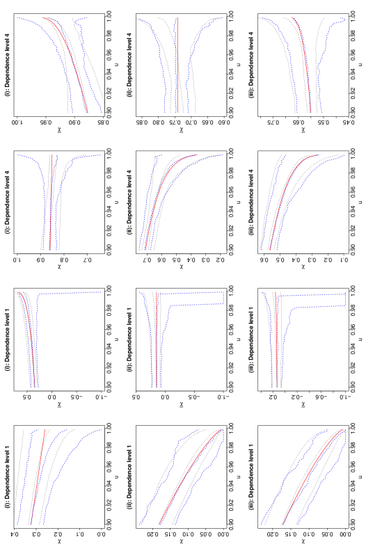
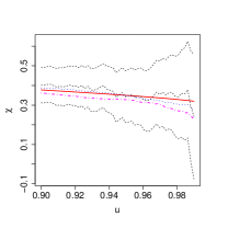
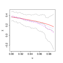
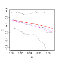
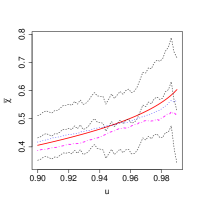
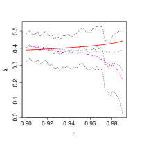
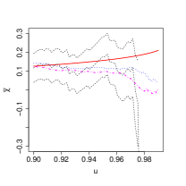
As a diagnostic for the model fit, we also consider the extremal dependence functions , defined in Section 4.3, and for (Coles et al.,, 1999). As , , as in (1.1), whilst . The value of thus gives some discrimination between different asymptotically dependent copulas, whilst can discriminate between different asymptotically independent copulas. As functions of , and are useful for checking model fits under either dependence scenario. Figure 1 displays pointwise medians and 90% confidence intervals of for each dependence structure and for both methods of inference. Small biases of the new model are typically offset by lower variability and better performance away from the diagonal, i.e., away from the region on which and focus.
6 Environmental application
We consider an oceanographic dataset comprising measurements of wave height, surge and wave period recorded at Newlyn, U.K., filtered to correspond to a 15-hour time window for approximate temporal independence, and previously analyzed by Coles and Tawn, (1994), Bortot et al., (2000) and Coles and Pauli, (2002). Coles and Tawn, (1994) noted the presence of seasonality, which was not taken into account in their, or subsequent, analyses; for ease of comparison we also ignore it. Coles and Tawn, (1994) used an asymptotically dependent model for these data, whilst Bortot et al., (2000) used an asymptotically independent Gaussian tail model. Coles and Pauli, (2002) employed a mixture-type model, able to encompass both dependence types, with asymptotic dependence arising at a boundary point. The literature appears to have reached a consensus that there is strong, but not overwhelming, evidence for asymptotic dependence between wave height and surge, and fairly strong evidence for asymptotic independence between the other two pairs.
Here we fit the simple symmetric model (5.2), with dependence threshold in likelihood (5.1). Marginal transformations to uniformity were carried out using the semiparametric procedure of Coles and Tawn, (1991) described in Section 5.1, but the dependence parameter estimates were almost the same using the fully empirical marginal transformation.
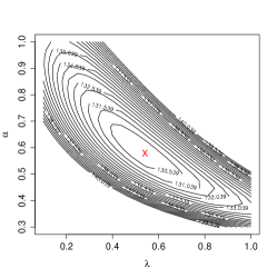
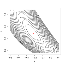
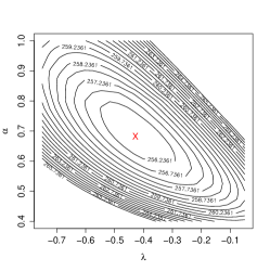
Table 2 gives maximum likelihood estimates and confidence intervals for the dependence parameters. The estimate suggests asymptotic dependence between wave height and surge, whilst the values and indicate asymptotic independence for the pairs involving period; this is supported by the confidence intervals. The likelihood surfaces plotted in Figure 2 show that the parameters are identifiable and give an appreciation of the joint asymptotic confidence regions. Figure 3 shows the empirical and fitted functions and , which suggest a reasonable fit to the data. Fits from the Heffernan–Tawn model are also displayed, conditioned on each variable in turn, and show potential discrepancies in the inferred strength of the dependence; by having only a single model, we can avoid such discrepancies and the need to decide which variable should be chosen for conditioning upon.
| Height–Surge | Height–Period | Surge–Period | |
|---|---|---|---|
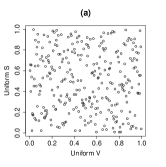
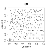
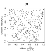
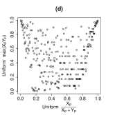
A further diagnostic is presented in Figures 4 (a) and (b), where “fitted” values of , and are plotted for the pairs height–surge and period–surge, on a uniform scale. Plots for height–period are similar to those for period–surge, and hence are omitted. Here , where is the fitted common pseudo-marginal distribution, and are the estimated true marginals. Points are plotted corresponding to where exceeds its 90% quantile. A lack of discernible patterns in Figures 4 (a) and (b) suggests that independence of and is a reasonable approximation. For comparison, Figures 4 (c) and (d) show equivalent plots with and on a uniform scale, ; this would be the approach to modelling under asymptotic dependence (Coles and Tawn,, 1991). The patterns in Figure 4 (c) suggest that asymptotic dependence is plausible, but that a higher threshold is required for independence of and . Figure 4 (d) shows that these variables would be dependent at any finite threshold.
7 Extensions and discussion
We have provided an alternative limit representation for bivariate extremes, which motivates a statistical model that can capture a wide spectrum of asymptotically dependent and asymptotically independent behaviour. An obvious question concerns extensions to higher dimensions. Assumption (1.4) is indeed simple to extend to the multivariate case: in some common margins, , the vector of positive random variables satisfies
| (7.1) |
at continuity points of , with placing mass on the interior of , and as in (1.5). This is a more general assumption than multivariate regular variation, the -dimensional extension of (1.3), that underpins much of classical multivariate extreme value theory (de Haan and de Ronde,, 1998).
However, the practical applicability of assumption (7.1) in higher dimensions is more limited than in the bivariate case. The assumption that the distribution of has mass on the interior of requires a certain regularity in the multivariate dependence structure, which is present in many theoretical examples, such as in the multivariate extensions of Examples 1–3, but often absent in datasets. For example, the data analyzed in Section 6 exhibited asymptotic dependence between one pair of variables, but asymptotic independence between the other two pairs. The only existing model which can handle this is that of Heffernan and Tawn, (2004). However there are obvious issues with the curse of dimensionality when using a semiparametric model for higher dimensions. The simulation study in Section 5 demonstrated a tendency for the semiparametric distribution estimator not to cover all parts of the plane, and this drawback would be exacerbated in higher dimensions.
We have assumed throughout that the radial variable is defined by a norm, following the development of much of classical multivariate extreme value theory. In fact the convexity property does not appear necessary, and some recent articles on multivariate extremes have shifted focus on to positive homogeneous functions rather than norms (e.g. Dombry and Ribatet,, 2015; Scheffler and Stoev,, 2015). For our model the convexity property of was used in some of the derivations; further work could explore more deeply the consequences of relaxing this assumption.
A simple extension to the practical modelling introduced in Sections 5 and 6 is to allow an asymmetric dependence structure. Our theoretical results in Section 4 already cover this scenario, but for simplicity of implementation we assumed the distribution of to be symmetric, so that the pseudo-marginals of were equal. As noted in Remark 1, the implied incorporates the necessary moment constraint for any .
In essence our approach is intermediate between assuming multivariate regular variation and the approach of Heffernan and Tawn, (2004). With the former, both the marginal distribution and the form of the normalization of each marginal variable, i.e., , are fixed. This is restrictive, but allows for simpler characterization of the consequences of the assumption. With the latter, the margins are fixed to be of exponential type, but the form of the normalization of each marginal variable, , is not fixed. This permits great flexibility in the variety of distributions that satisfy the assumption, but leaves possible limits, each with parameters to estimate, and a -dimensional empirical distribution. Our main assumption does not fix the form of the margins, but does fix the form of the normalization of the variables . This offers greater flexibility than multivariate regular variation, and although less flexible than the model of Heffernan and Tawn, (2004) has the benefit of giving only a single limit. In the bivariate case, model (4.1), inspired by (1.4), permits inference across both extremal dependence classes, with a smooth transition between them.
Acknowledgements
This work was undertaken whilst JLW was based at EPFL and the University of Cambridge. We thank the Swiss National Science Foundation for funding, and the referees and associate editor for comments that have greatly improved the work.
Appendix A Auxiliary results and proofs
A.1 Link between (1.4) and (3.2)
Proposition 5.
Let , , and assume that and have a joint density. Further assume to be in the domain of attraction of a generalized Pareto distribution, with normalization functions , . Then, provided that the limit on the right exists,
Proof.
Right to left: The statement on the right is equivalent to
Since both and equal zero, but the ratio of the derivatives has limit , the general form of l’Hôpital’s rule states that
Consequently, as ,
Left to right: Set in the left-hand statement, yielding
and note that . Then applying l’Hôpital’s rule again provides
∎
A.2 Proofs of Propositions 1–4
We prove Propositions 1–4, giving the values of , and claimed in Section 4.2. The following lemma on inversion of regularly varying functions will be useful throughout.
Lemma 1.
Suppose and is a slowly varying function such that defines a continuous strictly decreasing function from onto for some . Then we can find a slowly varying function defined on such that whenever . Furthermore as iff as (here can be any value in the extended range ).
The slowly varying functions and are de Bruijn conjugates.
Proof.
The expression defines a strictly increasing continuous map which is regularly varying with index (note that is slowly varying). Let denote the corresponding inverse, which is also regularly varying with index , and set for all ; it follows that is continuous and slowly varying. Setting we then get
The final part of the result follows (note that as since is slowly varying). ∎
Define as the reciprocal of defined in Section 4.2, i.e., , so that and . Using this notation equation (4.3) becomes
| (A.1) |
where the upper endpoint of the support is if and if ; and (4.4) becomes
| (A.2a) | ||||
| (A.2b) | ||||
The expressions and define continuous strictly decreasing functions from onto ; this observation can be used to help justify the conditions for Lemma 1 when it is used below.
From Condition 2, for , while Conditions 1 and 3 imply for some . Set . Now where is the continuous convex function defined by . It follows that is a closed subinterval of , so with , as defined in Section 4.2. Also note that ,
| is strictly decreasing on and strictly increasing on , | (A.3) |
and
| (A.4) |
The quantities and as given in Proposition 4 can be expressed
by Assumption 1, iff . We proceed with Cases 1–3 in turn, firstly by establishing the form of the quantile functions and , followed by proofs of the main Propositions concerning the behaviour of the joint survivor functions.
A.2.1 Case 1:
Recall the positive quantities defined in Remark 1; these can be expressed , and .
Proposition 6.
Let . Then there exist slowly varying functions , such that and for all . Furthermore and as .
Proof.
We have
As increases from to , decreases monotonically to ; hence increases monotonically to . Dominated convergence then gives
Since this limit is non-zero it follows that is slowly varying. The result for now follows from Lemma 1 (with ). The case is similar. ∎
Proof of Proposition 1.
Firstly suppose . From (A.2a), as defined in Proposition 1, is
Since , and (or ) has a non-zero limit as , we can bound uniformly away from for all sufficiently large . Furthermore Proposition 6 implies as . Applying dominated convergence and using the definitions of and then gives
The fact that this limit is non-zero implies is slowly varying. Now assume (the case can be handled similarly). Then
If then (A.4) gives
Combined with (A.1) and (A.2b) we thus have
The continuity of at gives as . Since we then get as . The result follows. ∎
Proof of Proposition 2.
Note that by Condition 3, . From (4.5) we get where
Now with equality iff . Since dominated convergence then gives
If then so as . Otherwise , in which case we can find so that when . Setting we then get
where and (positivity follows from Assumption 1 and the fact that the interval length ). As , and hence . A similar argument shows . ∎
A.2.2 Case 2:
Let and set . Then while (A.4) gives
| (A.5) |
The function is a positive, continuous and convex function on , with . Set and ; in particular, is a non-empty closed subinterval of . The general shape of and key properties of and can be deduced from (A.3):
-
C1: . Then is strictly decreasing on , is strictly increasing on and these quantities are equal when . It follows that and .
-
C2: . Then is strictly decreasing on and (a constant) on . Also is strictly increasing on and so is strictly increasing and not less than on ; hence is strictly increasing on . It follows that and (note that, which implies ).
-
C3: . By a similar argument to C2, and .
The main results in this case are built from the following lemma.
Lemma 2.
Suppose is continuous, is regularly varying at infinity with index , and for is a collection of closed intervals with the interval length and as . Define by
for each , and set . Then is regularly varying with index .
Note that by we mean that the Hausdorff distance between and tends to ; equivalently, the end points of converge to the end points of .
Proof.
For each set .
Claim 1: there exists such that when and . The continuity of implies is an open neighbourhood of . Since as it follows that for all sufficiently large .
Claim 2: there exists and such that for all . Choose and so that and . Then is an interval of length at least (recall that is an interval). Since is an interval converging to it follows that, for all sufficiently large , is an interval of length at least , which is contained in . We can then let be the infimum of , taken over all intervals of length at least ; this quantity is positive by Assumption 1.
Setting
we clearly have
| (A.6) |
Claim 3: there exists such that
| (A.7) |
Set . Since is regularly varying with index there exists such that
If then so
so, for any ,
When , Claim 2 then leads to
On the other hand, if then so
and thus, for any ,
When it follows that
When our estimates for and can be combined with (A.6) to give (A.7).
Let and . Choose so that . Since is regularly varying with index we can find such that
If and , Claim 1 gives and so
Integration then gives
| (A.8) |
Proposition 7.
Let . Then there exist slowly varying functions , such that and for all . Furthermore , are continuous, take values in and respectively, and satisfy and as .
Proof.
Proof of Proposition 3.
Setting
| (A.9) |
we have as (note that and are slowly varying). Furthermore (A.2b) gives
| (A.10) |
Now assume (the case can be handled similarly). Then so (A.3) gives . Furthermore, (recall the description of at the beginning of this section) so . Lemma 2 can now be applied to show that the integrals on the right hand side of (A.10) are regularly varying functions, the first with index and the second with index . By the forms of described in C1–C3 immediately preceding Lemma 2, the result follows. ∎
The fact that when in this case is given by the following.
Proposition 8.
If (equivalently ) and then .
A.2.3 Case 3: , with Assumption 2
Proposition 9.
Let . Then there exist slowly varying functions , such that and for all . Furthermore and as .
Proof.
Set . For we get
| (A.11) |
using (A.1). For we have (recall that ) so the integrand in (A.11) is bounded above by . Also note that as , so
As , dominated convergence now gives
Since this limit is non-zero it follows that is slowly varying. The result for now follows from Lemma 1 (with ). The case is similar. ∎
Let be a neighbourhood of on which is continuous; in particular, for .
Proof of Proposition 4.
Set so (A.2b) gives where
To consider firstly set . Since and as we get while as . As we can then choose so that whenever . For it follows that when ; in particular . Furthermore (A.3) implies is decreasing on . For we thus have
Therefore
Consider the new variable , and its inverse . We have (respectively ) when (respectively ). Thus
| (A.12a) | ||||
| (A.12b) | ||||
where
As we have so , uniformly for . Using Assumption 2 it follows that , uniformly for . Hence the integrands in (A.12) are uniformly bounded for all sufficiently large . Proposition 9 gives
| (A.13) |
Appendix B Derivations of ray dependence functions ( and ) and spectral density ()
Derivation of for
This follows simply by noting that Proposition 6 gives that marginal quantile functions are
for so that using the same dominated convergence arguments as in given in the proof of Proposition 1,
| (B.1) |
Therefore converges to with the form claimed in Remark 1.
Derivation of for
To derive , consider (B.1), with . This expression can be set equal to
By differentiating under the integral sign, we have
so that is recovered upon setting , and dividing by two. Thus we begin with
with . Differentiating with respect to yields
whilst differentiating what remains with respect to gives
Substituting in and noting that
gives
so that substituting and dividing by two yields
which is denoted in Remark 1.
Derivation of for
This follows firstly by noting that Proposition 9 gives that marginal quantile functions are
for . The ray dependence function can be found by following the proof of Proposition 4 through with these and , which reveals that
Therefore converges to with the form claimed in Remark 2.
References
- Abdous et al., (2005) Abdous, B., Fougères, A.-L., and Ghoudi, K. (2005). Extreme behaviour for bivariate elliptical distributions. The Canadian Journal of Statistics, 33(3):317–334.
- Beirlant et al., (2004) Beirlant, J., Goegebeur, Y., Segers, J., and Teugels, J. (2004). Statistics of Extremes. Wiley.
- Bortot et al., (2000) Bortot, P., Coles, S. G., and Tawn, J. A. (2000). The multivariate Gaussian tail model: an application to oceanographic data. Journal of the Royal Statistical Society, Series C, 49(1):31–49.
- Coles et al., (1999) Coles, S. G., Heffernan, J. A., and Tawn, J. A. (1999). Dependence measures for extreme value analyses. Extremes, 2(4):339–365.
- Coles and Pauli, (2002) Coles, S. G. and Pauli, F. (2002). Models and inference for uncertainty in extremal dependence. Biometrika, 89(1):183–196.
- Coles and Tawn, (1991) Coles, S. G. and Tawn, J. A. (1991). Modelling extreme multivariate events. Journal of the Royal Statistical Society, Series B, 53(2):377–392.
- Coles and Tawn, (1994) Coles, S. G. and Tawn, J. A. (1994). Statistical methods for multivariate extremes – an application to structural design (with discussion). Journal of the Royal Statistical Society, Series C, 43(1):1–48.
- Das and Resnick, (2014) Das, B. and Resnick, S. (2014). Generation and detection of multivariate regular variation and hidden regular variation. http://arxiv.org/abs/1403.5774.
- de Haan and de Ronde, (1998) de Haan, L. and de Ronde, J. (1998). Sea and wind: multivariate extremes at work. Extremes, 1(1):7–45.
- Dombry and Ribatet, (2015) Dombry, C. and Ribatet, M. (2015). Functional regular variations, Pareto processes and peaks over threshold. Statistics and its interface, to appear.
- Einmahl et al., (1997) Einmahl, J., de Haan, L., and Sinha, A. (1997). Estimation of the spectral measure of an extreme-value distribution. Stoch. Proc. Appl., 70:143–171.
- Heffernan, (2000) Heffernan, J. E. (2000). A directory of coefficients of tail dependence. Extremes, 3(3):279–290.
- Heffernan and Resnick, (2007) Heffernan, J. E. and Resnick, S. I. (2007). Limit laws for random vectors with an extreme component. Annals of Applied Probability, 17(2):537–571.
- Heffernan and Tawn, (2004) Heffernan, J. E. and Tawn, J. A. (2004). A conditional approach for multivariate extreme values (with discussion). Journal of the Royal Statistical Society, Series B, 66(3):497–546.
- Hult and Lindskog, (2002) Hult, H. and Lindskog, F. (2002). Multivariate extremes, aggregation and dependence in elliptical distributions. Advances in Applied Probability, 34(3):587–608.
- Leadbetter et al., (1983) Leadbetter, M. R., Lindgren, G., and Rootzén, H. (1983). Extremes and Related Properties of Random Sequences and Processes. Springer Verlag, New York.
- Ledford and Tawn, (1997) Ledford, A. W. and Tawn, J. A. (1997). Modelling dependence within joint tail regions. Journal of the Royal Statistical Society, Series B, 59(2):475–499.
- Liu and Tawn, (2014) Liu, Y. and Tawn, J. A. (2014). Self-consistent estimation of conditional multivariate extreme value distributions. Journal of Multivariate Analysis, 127:19–35.
- McNeil and Nešlehová, (2009) McNeil, A. J. and Nešlehová, J. (2009). Multivariate Archimedean copulas, -monotone functions and -norm symmetric distributions. Annals of Statistics, 37(5B):3059–3097.
- Mikosch, (2005) Mikosch, T. (2005). How to model multivariate extremes if one must? Statistica Neerlandica, 59(3):324–338.
- Peng and Qi, (2004) Peng, L. and Qi, Y. (2004). Discussion of A conditional approach for multivariate extreme values, by J. E. Heffernan and J. A. Tawn. Journal of the Royal Statistical Society, Series B, 66(3):541–542.
- Pickands, (1986) Pickands, J. (1986). The continuous and differentiable domains of attraction of the extreme value distributions. Ann. Probab., 14(3):996–1004.
- Ramos and Ledford, (2009) Ramos, A. and Ledford, A. W. (2009). A new class of models for bivariate joint tails. Journal of the Royal Statistical Society, Series B, 71(1):219–241.
- Resnick, (1987) Resnick, S. I. (1987). Extremes Values, Regular Variation and Point Processes. Springer Verlag, New York.
- Resnick, (2002) Resnick, S. I. (2002). Hidden regular variation, second order regular variation and asymptotic independence. Extremes, 5(4):303–336.
- Resnick, (2006) Resnick, S. I. (2006). Heavy Tail Phenomena: Probabilistic and Statistical Modeling. Springer, New York.
- Sabourin and Naveau, (2014) Sabourin, A. and Naveau, P. (2014). Bayesian Dirichlet mixture model for multivariate extremes: a re-parametrization. Computational Statistics and Data Analysis, 71:542–567.
- Scheffler and Stoev, (2015) Scheffler, H.-P. and Stoev, S. (2015). Implicit extremes and implicit max-stable laws. http://arxiv.org/abs/1411.4688.
- Shih and Louis, (1995) Shih, J. H. and Louis, T. A. (1995). Inferences on the association parameter in copula models for bivariate survival data. Biometrics, 51:1384–1399.
- Wadsworth and Tawn, (2013) Wadsworth, J. L. and Tawn, J. A. (2013). A new representation for multivariate tail probabilities. Bernoulli, 19(5B):2689–2714.