Harmonic-oscillator excitations of precise few-body wave functions

Abstract

A method for calculating the occupation probability of the number of harmonic oscillator (HO) quanta is developed for a precise few-body wave function obtained in a correlated Gaussian basis. The probability distributions of two- to four-nucleon wave functions obtained using different nucleon-nucleon ($NN$) interactions are analyzed to gain insight into the characteristic behavior of the various interactions. Tensor correlations as well as short-range correlations play a crucial role in enhancing the probability of high HO excitations. For the excited states of ⁴He, the interaction dependence is much less because high HO quanta are mainly responsible for describing the relative motion function between the $3N+N$ (³H$+p$ and ³He$+n$) clusters.

I Introduction

The nuclear shell model is a standard microscopic theory for describing a many-nucleon system. For doubly closed nuclei, first we consider the lowest HO state expressed with a single Slater determinant (SD), an antisymmetrized product of single-particle HO orbits. To take many-body correlations into account, multi-particle-multi-hole ($m$p-$m$h) configuration mixing calculations are performed by superposing many SD states that include higher HO excitations.

Thus far, the ab initio no-core shell model (NCSM) with modern nuclear forces has been developed extensively barrett13 . In the NCSM, all nucleons are active, but a crucial approximation is the truncation of maximum HO quanta, which determines the NCSM space. Compared to ordinary shell-model effective interactions, the use of realistic nuclear forces requires many SD states in higher major shells to reach convergence because of strong couplings between low- and high-momentum components arising from the tensor component and short-range repulsion of the nuclear force.

The HO expansion provides us with systematic and size extensive calculations, but it is not advantageous to describe the spatial extent of the wave function because of a rapid fall-off of the HO wave functions. If a system exhibits a cluster structure, the subsystems are localized and their relative motion wave function can have a long tail. For example, the first excited state of ¹⁶O is still difficult to reproduce by present large-scale shell-model calculations wloch05 ; maris09 . As shown in Refs. suzuki76 ; suzuki96 ; neff09 ; horiuchi14 , the cluster structure always induces extremely high HO quanta beyond the limitation of present computational resources. To make an efficient description of nuclear many-body systems using the HO expansion, it is useful to know how many HO excitations are required to account for those important correlations which are induced by the tensor force, the short-range repulsion, and the cluster structure.

Nowadays, precise wave functions of very light nuclei can be obtained using ab initio few-body methods. Though the few-body method can only be applied to very light nuclei, long-ranged asymptotics as well as short-range correlations are accurately described. Such few-body wave functions can provide important hints on how to tackle complicated many-body problems. Since the shell model and the few-body model are formulated in different frameworks, it is convenient to relate the few-body wave function to the HO wave function. For this purpose, by extending the formulation of Ref. suzuki96 , we calculate the occupation probability of the number of total HO quanta in the wave function obtained with an ab initio few-body method, in particular, using a correlated Gaussian (CG) basis with global vectors varga95 ; svm ; suzuki08 ; aoyama12 . We calculate the HO occupation probability of the wave functions of two- to four-nucleon systems and discuss its properties, especially focusing on the ⁴He system.

The nucleus ⁴He is an interesting example because important ingredients of many-nucleon dynamics show up in its spectrum. The ground state is strongly correlated due to the tensor component and short-range repulsion of the nuclear force. The tensor force induces a $D-$state mixing of approximately 14% kamada01 . Since the two nucleons cannot overlap with each other due to the short-range repulsion, the universal short-ranged behavior is found in the pair correlation functions forest96 ; feldmeier11 . In the excited states, the structure changes drastically. The first excited $0_{2}^{+}$ state of ⁴He is recognized to have a ³H$+p$ and ³He$+n$ ($3N+N$) cluster structure with $S$-wave relative motion hiyama02 . The negative-parity states are located at just a few MeV above the $0_{2}^{+}$ state and are considered to be parity-inverted partners of the $0_{2}^{+}$ state. They have the intrinsic structure of $3N+N$ with $P$-wave relative motion horiuchi08 . Thus, ⁴He has a similarity to ¹⁶O suzuki76 that exhibits a ${}^{12}{\rm C}+\alpha$ cluster structure in its spectrum.

The analysis of the oscillator excitations will be useful for developing and improving a truncation scheme for the model space in, e.g., ab initio NCSM barrett13 , importance-truncated NCSM roth07 ; forssen13 , symmetry-adapted no-core shell model dytrych07 , Monte Carlo shell model shimizu13 as well as a model approach like the tensor-optimized shell model myo07 .

The paper is organized as follows. Section II.1 gives a basic formula to calculate the occupation probability of the HO quanta in the CG basis. Section II.2 defines the Hamiltonian and the CG basis, and briefly explains how we obtain the precise few-body wave functions. Section III demonstrates the HO occupation probability distributions for two- to four-nucleon systems. Four different potentials are employed in order to examine how the HO distribution reflects the characteristics of the nuclear force. In Sec. III.1, we discuss the role of the HO quanta higher than the lowest $(0s)^{N}$ configuration, focusing on the relationship with the short-range repulsion and tensor correlations in the ground state of ⁴He. Long-ranged cluster correlations in the excited states of ⁴He are discussed in Sec. III.2. Section III.3 discusses the parity-inverted partners of the first excited state of ⁴He. The summary is given in Sec. IV. An appendix details a method for calculating the probability of the HO quanta.

II Formulation

II.1 Harmonic-oscillator occupation probability

Let $\Psi$ denote an $N$-nucleon wave function that is spurious center-of-mass (c.m.) motion free. The occupation probability $P_{Q}$ of the $Q\,\hbar\omega$ components in $\Psi$ is calculated using an integral of the projection-operator type

$$P_{Q}=\frac{1}{2\pi}\int_{0}^{2\pi}d\theta\,\text{e}^{-iQ\theta}\left<\Psi\right|\text{e}^{i\theta\mathcal{O}}\left|\Psi\right>,$$ (1)

where $\mathcal{O}$ is an operator that counts the number of HO quanta

$$\mathcal{O}=\sum_{i=1}^{N-1}\left(\frac{1}{\hbar\omega}H_{\rm HO}(i)-\frac{3}{2}\right).$$ (2)

Here $H_{\rm HO}(i)$ is the HO Hamiltonian for the $i$th relative coordinate. See the appendix for details. The method for calculating $P_{Q}$ was developed for microscopic multicluster wave functions in Ref. suzuki96 . We extend it to the case where $\Psi$ is given in terms of a combination of CG basis functions.

The CG is constructed from the generating function varga95 ; svm

$$g(\bm{s};A,\bm{x})=\exp\left(-\frac{1}{2}\tilde{\bm{x}}A\bm{x}+\tilde{\bm{s}}\bm{x}\right),$$ (3)

where the $(N-1)\times(N-1)$ matrix $A$ is positive-definite and symmetric, $\bm{s}$ is a column vector of an $(N-1)$ dimension to describe the angular motion of the system, and $\bm{x}$ is a column vector of an $(N-1)$ dimension whose element is the 3-dimensional relative coordinate $\bm{x}_{i}$. The transpose of a matrix is indicated by a tilde symbol. Both $A$ and $\bm{s}$ are variational parameters, which makes the CG flexible and easily adapted to few-body problems. To calculate the quantity (1) with the CG, we start from the matrix element of $\text{e}^{i\theta\mathcal{O}}$ between the generating functions (3). As detailed in the appendix, the required matrix element reads

$$\left<g(\bm{s}^{\prime};A^{\prime},\bm{x})\right|\text{e}^{i\theta\mathcal{O}}\left|g(\bm{s};A,\bm{x})\right>$$

$$=\left(\frac{(2\pi)^{N-1}\det\Gamma}{\det B\det C}\right)^{\frac{3}{2}}\exp\left(-\frac{1}{2}\tilde{\bm{s}}G\bm{s}+\frac{1}{2}\tilde{\bm{v}}B^{-1}\bm{v}\right),$$ (4)

where $B=D+A^{\prime}$, $\bm{v}=z\Gamma C^{-1}\bm{s}+\bm{s}^{\prime}$, and $z=\text{e}^{i\theta}$. The matrices $\Gamma,C,D$, and $G$ are defined in the appendix. Once the matrix element between the CG bases is obtained as a function of $\theta$, the integration in Eq. (1) is performed numerically.

II.2 Few-body wave functions

II.2.1 Hamiltonian

The Hamiltonian of the $N$-nucleon system is composed of the kinetic energy, two-body $NN$ interaction, and three-body interaction (3NF) terms

$$H=\sum_{i=1}^{N}T_{i}-T_{\rm cm}+\sum_{i<j}v_{ij}+\sum_{i<j<k}v_{ijk}.$$ (5)

The c.m. kinetic energy is subtracted and no spurious c.m. motion is involved in the calculation. The inputs used in this paper are $\hbar^{2}/m=41.47106$ MeV fm² and $e^{2}=1.440$ MeV fm. The proton mass and neutron mass are taken to be equal.

We adopt (i) Minnesota (MN) MN , (ii) Afnan-Tang S3 (ATS3) ATS3 , (iii) G3RS G3RS , and (iv) AV8^′ AV8p potential models as the $NN$ interaction. A central 3NF hiyama02 is added together with the realistic G3RS and AV8^′ potentials in order to reproduce the binding energies of ³H and ⁴He. The MN potential is often used in microscopic cluster-model calculations. Though it has only a central term, the potential reproduces the binding energies of $N=2-6$ systems fairly well varga95 . The ATS3 potential also has only the central term but contains a strong short-range repulsive core. The AV8^′ potential consists of central, spin-orbit, and tensor components, as well as has strong short-range repulsion. The G3RS potential is somewhat softer than AV8^′ and gives a smaller $D$-state probability. The $\bm{L}^{2}$ and quadratic $\bm{L}\cdot\bm{S}$ terms in the G3RS potential are ignored.

II.2.2 Correlated Gaussians and global vectors

The wave function $\Psi$ is given as a combination of the basis functions expressed in the $LS$ coupling scheme

$$\Phi_{(LS)JM_{J}TM_{T}}=\mathcal{A}\left[F_{L}(\bm{x})\chi_{S}^{\text{(spin)}}\right]_{JMJ}\eta_{TM_{T}}^{\text{(isospin)}},$$ (6)

where $\mathcal{A}$ is the antisymmetrizer, and the square brackets, $[\dots]$, denote the angular momentum coupling. The spin function is given in a successive coupling scheme

$$\chi^{\text{(spin)}}_{SM_{S}}=[\dots[[\chi_{1/2}(1)\chi_{1/2}(2)]_{S_{12}}\chi(3)]_{S_{123}}\dots]_{SM_{S}}.$$ (7)

The isospin wave function has exactly the same form as the spin part. All possible intermediate spins and isospins are included in the basis set. The orbital part is represented by the CG with two global vectors

$$F_{(L_{1}L_{2})LM_{L}}(u_{1},u_{2},A,\bm{x})$$

$$=\exp\left(-\frac{1}{2}\tilde{\bm{x}}A\bm{x}\right)\left[\mathcal{Y}_{L_{1}}(\tilde{u}_{1}\bm{x})\mathcal{Y}_{L_{2}}(\tilde{u}_{2}\bm{x})\right]_{LM_{L}}$$ (8)

with a solid harmonic

$$\mathcal{Y}_{\ell m}(\bm{r})=r^{\ell}Y_{\ell m}(\hat{\bm{r}}),$$ (9)

where $u_{i}$ is an $(N-1)$-dimensional column vector and $\tilde{u}_{i}\bm{x}$ is called a global vector that describes the rotational motion of the system. The off-diagonal matrix elements of $A$ explicitly describe correlations among the particles. The matrix element of the Hamiltonian between the CG of Eq. (8) can be obtained analytically from the one between the generating functions (3) in a systematic, algebraic procedure prescribed in Refs. svm ; suzuki08 ; aoyama12 . The CG basis (8) has the great advantage that its functional form remains unchanged under a coordinate transformation, thereby facilitating easily operations such as the ones involved in channel rearrangements and permutations, etc. This flexibility enables us to apply the CG approach to many quantum-mechanical few-body problems. See Ref. mitroy13 for recent various applications of the CG.

The ground states of ^2,3H, ⁴He and the excited states of ⁴He are obtained using the stochastic variational method varga95 ; svm . Though all the excited states of ⁴He are above the ³H+$p$ threshold, we describe them in the square-integrable CG basis functions. Since they have relatively small decay widths ranging from 0.5 to 2 MeV tilley92 , the bound-state approximation works reasonably well as discussed in Ref. horiuchi13a . More details of calculations are given in Refs. suzuki08 ; horiuchi08 ; horiuchi13b .

III Results and discussions

III.1 Ground states: tensor and short-range correlations

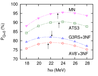
Figure 1: (Color online) $\hbar\omega$ dependence of the occupation probability of the lowest HO quantum in the ground state of ⁴He. The arrow indicates the $\hbar\omega$ value that is employed to calculate $P_{Q}$ values of ⁴He. See text for detail.

Figure 1 displays the probability of the lowest HO quantum, $P_{0}$, for the ground state of ⁴He as a function of the oscillator frequency $\hbar\omega$. We see moderate $\hbar\omega$ dependence of $P_{0}$ in all the potential models. Since the $P_{Q}$ distribution depends on $\hbar\omega$, we fix it by requiring that the lowest shell-model configuration, $(0s)^{N}$, for the fixed $\hbar\omega$ reproduces the root-mean-square (rms) matter radius of the precise wave function. This is reasonable because the $(0s)^{N}$ configuration is the dominant component of the wave function for $s$-shell nuclei. The $\hbar\omega$ values determined for ⁴He are 23.2, 23.4, 22.2, and 21.6 MeV for MN, ATS3, G3RS+3NF, and AV8^′+3NF potentials, respectively. The $P_{0}$ values calculated with these $\hbar\omega$ values are close to the maximum values in Fig. 1.

Table 1: Ground-state energies ($E$) and rms matter radii ($r_{m}$) of two- to four-nucleon systems calculated with different potential models: (i) MN, (ii) ATS3, (iii) G3RS+3NF, and (iv) AV8^′+3NF potentials. The $D$-state probability $P(D)$ and the occupation probability $P_{0}$ of the $0\,\hbar\omega$ component are given in percents. $M_{Q}$ and $\sigma_{Q}$ denote the average and standard deviation of the $P_{Q}$ distribution.

			$E$(MeV)	$r_{m}$(fm)	$P(D)$(%)	$P_{0}$(%)	$M_{Q}$	$\sigma_{Q}$
2H	(i)		$-$2.20	1.95	0.00	89.6	0.534	1.95
($1^{+}0$)	(ii)		$-$2.22	1.94	0.00	89.4	0.692	3.77
	(iii)		$-$2.28	1.98	4.78	86.9	1.27	5.80
	(iv)		$-$2.24	1.96	5.77	85.5	1.57	6.84
3H	(i)		$-$8.38	1.71	0.00	90.8	0.409	1.70
($\tfrac{1}{2}^{+}\tfrac{1}{2}$)	(ii)		$-$8.76	1.67	0.00	89.7	0.787	3.99
	(iii)		$-$8.35	1.74	7.10	84.9	1.52	5.96
	(iv)		$-$8.41	1.70	8.69	83.1	1.92	7.08
4He	(i)		$-$29.94	1.41	0.00	95.4	0.263	1.48
($0_{1}^{+}0$)	(ii)		$-$30.83	1.42	0.00	90.4	0.934	4.00
	(iii)		$-$28.56	1.47	11.42	82.1	1.96	5.98
	(iv)		$-$28.43	1.45	14.07	79.1	2.59	7.31

Table 1 summarizes the calculated energy $E$, rms matter radius $r_{m}$, $D$-state probability $P(D)$, and $P_{0}$ of the ground state of ²H, ³H, and ⁴He for the different potential models. All the interactions give approximately the same $E$ and $r_{m}$ but quite different $P(D)$. The MN potential, which is the softest among the four potentials, gives the largest $P_{0}$ of approximately 95% for ⁴He. The $N=2-4$ wave functions with the MN potential are well described by the $(0s)^{N}$ configurations. When the other interactions are employed, the mixing of higher-$Q$ components becomes important. When a realistic potential is used, the deviation from the $(0s)^{N}$ structure is the largest in ⁴He, which is the most tightly bound and has the largest $D$-state probability, as a result of the effects of short-range and tensor correlations. The ground state of ⁴He obtained with the AV8^′+3NF interaction predicts at most 80% of the $(0s)^{4}$ configuration.

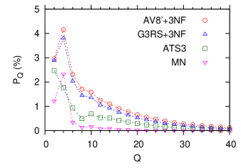
Figure 2: (Color online) Occupation probability distributions of the total HO quanta for the ground state of ⁴He calculated with different potential models. $P_{0}$ is not shown in the figure but given in Table 1. $P_{Q}$ values are connected by dotted lines to guide the eye.

Figure 2 plots $P_{Q}\,(Q>0)$ of ⁴He. Consistently with the $M_{Q}$ and $\sigma_{Q}$ values in Table 1, a harder interaction leads to $P_{Q\neq 0}$ that is more enhanced and extended to larger $Q$. In the case of the MN potential, $P_{Q}$ is found to be about 1% to 2% for $Q=2$ and $4$, but it diminishes rapidly with increasing $Q$. Since no short-range repulsion is present in the MN potential, the configurations contributing to $P_{2}$ and $P_{4}$, e.g., $(0s)^{3}(1s)$ for $Q=2$ and $(0s)^{2}(1s)^{2}$, $(0s)^{3}(2s)$ for $Q=4$ are expected to improve the tail of the wave function that cannot be described with $(0s)^{4}$ alone. One may wonder why $P_{2}$ is smaller than $P_{4}$. We recalculate $P_{Q}$ using smaller $\hbar\omega$ to describe the tail part more efficiently. For $\hbar\omega$ less than 20 MeV, the $P_{Q}$ distribution shows a monotonous decrease with increasing $Q$. The $P_{Q}$ values for small $Q$ depend on the choice of $\hbar\omega$. We will discuss this later in this section. With the ATS3 potential, $P_{Q}$ decreases monotonously up to $Q=8$ and exhibits a bump at $Q=10$ with a long tail extending to more than $Q=30$, which is apparently due to the short-range repulsion. The G3RS+3NF and AV8^′+3NF potentials give a very similar pattern characterized by large and very extended $P_{Q}$ distributions. The probability is still 1.6% at $Q=10$ and 0.7% at $Q=20$ when the AV8^′+3NF potential is used.

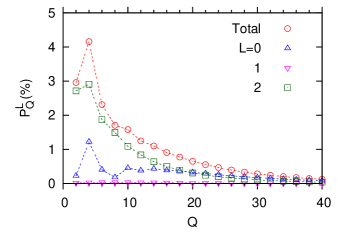
Figure 3: (Color online) Angular momentum decomposition of the occupation probability of the total HO quanta for the ground state of ⁴He. $P^{L}_{0}$ values in percents are 79.1, 0, 0 for $L=0,1,2$, respectively. The AV8^′+3NF potential is used.

To discuss whether the short-range repulsion or the tensor component in the $NN$ interaction is important in determining the $P_{Q}$ distribution, we decompose $P_{Q}$ according to the total orbital angular momentum $L$. The ground-state wave function of ⁴He is expressed in the notation of Eq. (6) as

$$\Psi=\sum_{L=0,1,2}\sum_{i}C_{L}^{(i)}\Phi_{(LL)0000}^{(i)},$$ (10)

where the amplitude $C_{L}^{(i)}$ of the $i$th basis state $\Phi_{(LL)0000}^{(i)}$ satisfies $\sum_{L=0,1,2}\sum_{i}(C_{L}^{(i)})^{2}=1$. The $P_{Q}$ is decomposed to a sum of $P_{Q}^{L}$ that is defined by

$$P_{Q}^{L} =\frac{1}{2\pi}\sum_{i}(C_{L}^{(i)})^{2}\int_{0}^{2\pi}d\theta\,\text{e}^{-iQ\theta}$$

$$\times\left<\Phi_{(LL)0000}^{(i)}\right|\text{e}^{i\theta\mathcal{O}}\left|\Phi_{(LL)0000}^{(i)}\right>.$$ (11)

Figure 3 displays $P_{Q}^{L}$ of the ground state of ⁴He calculated with the AV8^′+3NF potential. The $P^{1}_{Q}$ is negligibly small because the $L=1$ component occupies only 0.37% of the total wave function horiuchi13b . The $L=2$ component can couple with the $L=0$ configurations through the tensor force that induces a major shell mixing in the wave function. The $P_{Q}^{2}$ dominates up to $Q=18$, where the $P_{Q}^{0}$ gives an equal contribution. The $P^{0}_{Q}$ distribution shows a bump at $Q=10$ with a long tail similarly to the ATS3 potential case. This suggests that the bump and tail behavior in the $L=0$ component is due to the short-range repulsion. Both the tensor and short-range characters of the $NN$ potential make the convergence of conventional shell-model calculations very slow.

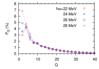
Figure 4: (Color online) $\hbar\omega$ dependence of the occupation probability of the total HO quanta with $Q>0$ for the ground state of ⁴He. The AV8^′+3NF potential is used.

Figure 4 presents how the probability distribution changes with different $\hbar\omega$ values. Though $P_{2}$ depends on $\hbar\omega$, the dependence of the sum of $P_{0}$ and $P_{2}$ is much weaker. This is understood as follows. Since the main role of the configurations with $Q=0$ and 2 is considered to describe the mean-field correlation of the system, each of $P_{Q}$ values may depend on a choice of $\hbar\omega$ but the sum of them may not so much. A weaker dependence of $P_{Q}$ at $Q=4$ and 6 reflects the dominance of the tensor correlations. Finally no $\hbar\omega$ dependence is found for $Q>6$. The higher-$Q$ components are always present and remain unchanged for different choices of $\hbar\omega$.

The mechanism responsible for enhancing the high-$Q$ components is different for the short-range repulsion and the tensor correlations of the realistic $NN$ interaction. The total number of HO quanta $Q$ is a sum of the HO quanta, $\sum_{i=1}^{N}(2n_{i}+l_{i})$, where $n_{i}$ and $l_{i}$ are respectively the principal and azimuthal quantum numbers of the HO wave function of the $i$th nucleon. Since no spurious c.m. motion is included, the sum ranges over all the nucleons. As shown in Refs. forest96 ; kamada01 ; feldmeier11 , the short-range repulsion makes a strong depression at short distances in the pair correlation function. In the HO expansion, this depression of the pairwise relative wave functions at short distances is taken care of by superposing many HO wave functions that have larger $n_{i}$ with the same $l_{i}$, which obviously leads to the large-$Q$ components. On the other hand, the tensor correlations induce high-$Q$ components, because of the couplings between the HO wave functions with different $l_{i}$.

The $P_{Q}$ distribution actually reflects the momentum distribution. As we have already mentioned, the realistic interaction demands HO functions with large $Q$ in the coordinate space. Noting that the Fourier transform of the HO function in the coordinate space is again the HO function in the momentum space, the HO functions with large $Q$ certainly contain large-momentum components. Refs. schiavilla07 ; horiuchi07 ; suzuki08 ; feldmeier11 showed that the momentum distribution has a long tail due to the tensor and short-range correlations. The HO functions with large $Q$ play a role in enhancing the high momentum tail of the momentum distribution, whereas those with small $Q$ describe the mean-field structure below the Fermi momentum.

Since the inclusion of all the high-$Q$ components is not practical for heavier nuclei, an effective interaction starting from the realistic $NN$ interaction is usually employed to accelerate the convergence. Such effective interactions are derived in several approaches, for example, Lee-Suzuki transformation suzuki80 , unitary correlation operator method (UCOM) feldmeier98 ; neff03 , and similarity renormalization group bogner07 . A softened interaction always improves the energy convergence roth10 ; bogner10 and succeeds to reproduce some low-lying spectra of light nuclei. See Ref. barrett13 for many such applications in the NCSM framework.

III.2 First excited state of ⁴He: cluster correlation

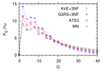
Figure 5: (Color online) Occupation probability distributions of the total HO quanta for the first excited state of ⁴He.

The $P_{Q}$ distribution of the excited state of ⁴He shows a pattern quite different from that of the ground state. Figure 5 plots $P_{Q}$ of the first excited $J^{\pi}T=0^{+}0$ state calculated with the four interaction models. The $P_{0}$ value almost vanishes, obviously because the state is orthogonal to the ground state whose major configuration is $(0s)^{4}$. The distribution is less interaction-dependent at $Q<10$ compared to that of the ground state, which appears to be attributed to the weakly bound $3N+N$ cluster structure of the first excited state hiyama02 ; horiuchi08 . Assuming that the scattering length between $3N$ and $N$ is much larger than its effective range, the system does not depend much on the detail of the interaction. This universal property is found in atomic systems and its similarity to the first excited $0^{+}0$ state is discussed in Ref. hiyama12 . Beyond $Q=10$, $P_{Q}$ decreases monotonously and very slowly with increasing $Q$, and the values of $M_{Q}$ and $\sigma_{Q}$ in the case of the AV8^′+3NF potential turn out to be 15.3 and 13.3, respectively. Appreciable probability still exists even at $Q=30$, which is too large for standard shell-model calculations to incorporate jurgenson11 . From the angular momentum decomposition of $P_{Q}$ we find out that the $L=0$ component, $P^{0}_{Q}$, dominates over the whole $Q$ region. This is also consistent with the fact that the $0_{2}^{+}$ state has an $S$-wave $3N+N$ cluster structure. If a state has a cluster structure, its $P_{Q}$ distribution spreads over large $Q$ because describing the relative motion between the clusters up to the asymptotic region requires configurations with large $Q$, even though the intrinsic wave functions of the clusters do not contain high HO excitations suzuki96 . Other well-known examples, which support this fact, include the Hoyle state of ¹²C suzuki96 ; neff09 and the first excited state of ¹⁶O suzuki76 ; horiuchi14 .

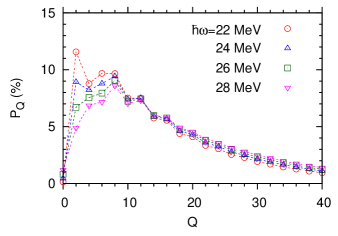
Figure 6: (Color online) $\hbar\omega$ dependence of the occupation probability of the total HO quanta for the first excited state of ⁴He. The AV8^′+3NF potential is used.

One may think that the first excited state of ⁴He can be described well in a shell model by choosing $\hbar\omega$ appropriately. To examine this question more closely, we exhibit the $\hbar\omega$ dependence of $P_{Q}$ in Fig. 6. The probability for $Q<10$ depends on $\hbar\omega$, but no practical dependence is found beyond this $Q$ value. Since the occupation probability is still significant for $Q>8$, we conclude that no appropriate choice for $\hbar\omega$ exists to describe the cluster state in the conventional shell-model truncation. Since the maximum major shell in shell-model calculations cannot be taken sufficiently large at present, it is reasonable to improve the wrong asymptotic behavior of the HO basis by combining with some other methods such as the resonating group method baroni13 ; quaglioni13 .

III.3 Inversion doublets in ⁴He

As shown in Ref. horiuchi08 , the first excited state of ⁴He has those negative-parity partners that have basically the same intrinsic structure. If a system has a two-cluster structure consisting of asymmetric subsystems, both positive and negative parity states may be found around the relevant threshold energy. A well-known example is ¹⁶O with a ¹²C$+\alpha$ structure suzuki76 ; horiuchi14 . As a ‘mini’ version of ¹⁶O  the spectrum of ⁴He has some similarity to that of ¹⁶O. Because of the spin-isospin coupling of $3N+N$ clusters, seven negative-parity states appear in ⁴He above the first excited $0^{+}0$ state, as shown in calculations with the AV8^′+3NF potential horiuchi13a .

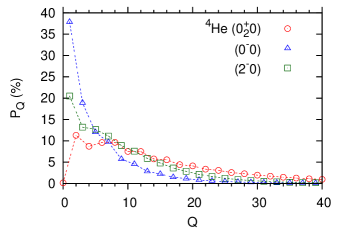
Figure 7: (Color online) Occupation probability distributions of the HO quanta for the excited states of ⁴He. The AV8^′+3NF potential is used.

Figure 7 plots the $P_{Q}$ values of the $0^{-}0\,(21.01\,\text{MeV})$ and $2^{-}0\,(21.84\,\text{MeV})$ states that are identified as the parity-inverted partners horiuchi08 . For the sake of comparison, the $P_{Q}$ of the positive-parity partner, the $0^{+}_{2}0$ state, is also drawn. Though the HO occupation probability is widely distributed to high $Q$ values, the $P_{1}$ value of the $0^{-}$ state is 37.9%, as well as the $M_{Q}$ and $\sigma_{Q}$ values are 5.42 and 6.36, respectively. These values are not as large as the corresponding values for the $0^{+}_{2}0$ state. Since it has a significant overlap with the 1p-1h configurations, the $0^{-}0$ state is expected to be described fairly well in large-scale shell-model calculations. Compared to the $0^{-}0$ state, the $P_{Q}$ distribution of the $2^{-}0$ state is closer to that of the $0^{+}0$: the $P_{1}$ value is 20.5%, while the $M_{Q}$ and $\sigma_{Q}$ values grow to 8.72 and 8.00, respectively. Because of the $P$-wave centrifugal barrier between $3N$ and $N$ clusters, the $2^{-}0$ state shrinks compared to the $0^{+}_{2}0$ state and consequently the distribution of $P_{Q}$ is shifted to lower $Q$ values than that of the $0^{+}_{2}0$ state.

IV Summary

We have formulated a method for calculating the occupation probability of the number of total harmonic-oscillator (HO) quanta $Q$ to shed light on various types of nuclear correlations. We have analyzed the occupation probability distributions of the precise wave functions of $s$-shell nuclei that are obtained in the correlated Gaussian basis employing four kinds of interactions.

The HO probability distributions show quite different behavior reflecting the characteristics of the interaction employed. In the case of the ground state of ⁴He, the tensor force significantly enhances the probability below $Q=20$. The short-range repulsion also plays an important role in mixing configurations with more than $Q=10$ excitations. For the excited states of ⁴He, the occupation probability is widely distributed to large $Q$ values and does not depend so much on the detail of the interaction. Configurations with a higher number of HO quanta are needed to describe the tail of the relative motion between the $3N$ and $N$ clusters. In conformity to the parity-inverted doublet structure, the similarity of the HO distribution of the first excited $J^{\pi}T=0^{+}0$ state to that of the negative-parity excited states with $0^{-}0$ and $2^{-}0$ is discussed.

We find that all the probability distributions beyond $Q=10$ are insensitive to the choice for the HO oscillator frequency $\hbar\omega$. These high-$Q$ components in the wave function always exist irrespective of whether the interaction is effective or realistic and thereby lead to the difficulty or extremely slow convergence in describing the cluster structure in the HO basis. The analysis presented here is useful for confirming that the occupation probability distribution in fact reflects important correlations and various kinds of structure of the nuclear wave functions. This analysis will be useful for providing a hint on how to develop an improved truncation scheme for huge shell-model spaces.

Appendix A Matrix element for the projection operator of number of HO quanta

We define the Jacobi coordinate and the corresponding reduced mass as

$$\bm{x}_{i}=\frac{1}{i+1}\sum_{j=1}^{i}\bm{r}_{j}-\bm{r}_{i+1},\quad\mu_{i}=\frac{i}{i+1}m$$ (12)

with $i=1,\dots,N-1$, where $\bm{r}_{j}$ is the $j$th nucleon coordinate. Letting $\bm{\pi}_{i}$ denote the momentum conjugate to $\bm{x}_{i}$, the HO Hamiltonian $H_{\rm HO}(i)$ in Eq. (2) reads

$$H_{\rm HO}(i)=\frac{\bm{\pi}_{i}^{2}}{2\mu_{i}}+\frac{1}{2}\mu_{i}\omega^{2}\bm{x}_{i}^{2}.$$ (13)

We evaluate the matrix element of $\text{e}^{i\theta\mathcal{O}}$ between the generating functions of the CG (3) in three steps. First, we rewrite the generating function in a multiple-integral form of a product of Gaussian wave-packets. Next, we act with $\text{e}^{i\theta\mathcal{O}}$ on the Gaussian wave-packets. Finally, the multiple-integral is performed analytically, which leads to the required matrix element.

Let $\psi_{\bm{R}_{i}}^{\gamma_{i}}(\bm{x}_{i})$ denote a Gaussian wave-packet centered at $\bm{R}_{i}$ with a width parameter $\gamma_{i}$

$$\psi_{\bm{R}_{i}}^{\gamma_{i}}(\bm{x}_{i})=\left(\frac{\gamma_{i}}{\pi}\right)^{3/4}\exp\left(-\frac{\gamma_{i}}{2}(\bm{x}_{i}-\bm{R}_{i})^{2}\right).$$ (14)

The first step is to use the identity varga95

$$g(\bm{s};A,\bm{x}) =\left[\frac{(\det\Gamma)^{3}}{(4\pi)^{N-1}(\det(\Gamma-A))^{2}}\right]^{\frac{3}{4}}\exp\Big{(}-\frac{1}{2}\tilde{\bm{s}}(\Gamma-A)^{-1}\bm{s}\Big{)}$$

$$\quad\times\int d\bm{R}\,g(\Gamma(\Gamma-A)^{-1}\bm{s};A(\Gamma-A)^{-1}\Gamma,\bm{R})\prod_{i=1}^{N-1}\psi_{\bm{R}_{i}}^{\gamma_{i}}(\bm{x}_{i}),$$ (15)

where $\bm{R}$ stands for an ($N-1$)-dimensional column vector whose $i$th element is $\bm{R}_{i}$ and $d\bm{R}=d\bm{R}_{1}d\bm{R}_{2}\ldots d\bm{R}_{N-1}$. $\Gamma$ is an $(N-1)\times(N-1)$ diagonal matrix whose element is chosen to be

$$\Gamma_{ij}=\gamma_{i}\delta_{i,j}=\frac{\mu_{i}\omega}{\hbar}\delta_{i,j}.$$ (16)

The second step is to use the identity (see Eq. (5) of Ref. suzuki96 ), which makes it possible to obtain

$$\exp\left(i\theta\left[\frac{1}{\hbar\omega}H_{\rm HO}(j)-\frac{3}{2}\right]\right)\psi_{\bm{R}_{j}}^{\gamma_{j}}(\bm{x}_{j})$$

$$\quad=\exp\left(-\frac{\gamma_{j}}{4}(1-z^{2}){\bm{R}_{j}^{2}}\right)\psi_{z\bm{R}_{j}}^{\gamma_{j}}(\bm{x}_{j}),$$ (17)

where $z=\text{e}^{i\theta}$. The operation of $\text{e}^{i\theta\mathcal{O}}$ on the product of the Gaussian wave-packets is then given in a simple form:

$$\text{e}^{i\theta\mathcal{O}}\prod_{i=1}^{N-1}\psi_{\bm{R}_{i}}^{\gamma_{i}}(\bm{x}_{i})=\exp\left(-\frac{1}{4}(1-z^{2})\tilde{\bm{R}}\Gamma\bm{R}\right)\left(\frac{{\rm det}\Gamma}{\pi^{N-1}}\right)^{3/4}\exp\left(-\frac{1}{2}\tilde{\bm{x}}\Gamma\bm{x}+z\tilde{\bm{R}}\Gamma\bm{x}-\frac{1}{2}z^{2}\tilde{\bm{R}}\Gamma\bm{R}\right).$$ (18)

The third step for obtaining $e^{i\theta\mathcal{O}}g(\bm{s};A,\bm{x})$ is to substitute the above result into Eq. (15) and integrate over $\bm{R}$, which leads to the following compact result expressed again in terms of the generating function (3) of CG:

$$\text{e}^{i\theta\mathcal{O}}g(\bm{s};A,\bm{x})$$

$$\ =\left(\frac{\det\Gamma}{\det C}\right)^{3/2}\exp\left(-\frac{1}{2}\tilde{\bm{s}}G\bm{s}\right)g(z\Gamma C^{-1}\bm{s};D,\bm{x}),$$ (19)

where the matrices $C,\,D$, and $G$ are given by

$$C =A+\frac{1+z^{2}}{2}(\Gamma-A),$$

$$D =\left(A+\frac{1-z^{2}}{2}(\Gamma-A)\right)C^{-1}\Gamma,$$ (20)

$$G =-\frac{1-z^{2}}{2}C^{-1}.$$

It is easy to derive Eq. (4) using the result above.

A calculation of the matrix element of $\text{e}^{i\theta\mathcal{O}}$ between the CG (8) is therefore reduced to that of the overlap matrix element of the CG. See Refs. svm ; suzuki08 ; aoyama12 that detail this process. An explicit form for the matrix element reads

$$\left<F_{(L_{3}L_{4})LM}(u_{3},u_{4},A^{\prime},\bm{x})|{\rm e}^{i\theta\mathcal{O}}|F_{(L_{1}L_{2})LM}(u_{1},u_{2},A,\bm{x})\right>$$

$$\quad=\left(\frac{{\rm det}\,\Gamma\ {\rm det}\,(A+A^{\prime})}{{\rm det}B\,{\rm det}C}\right)^{3/2}\left<F_{(L_{3}L_{4})LM}(u_{3},u_{4},A^{\prime},\bm{x})|F_{(L_{1}L_{2})LM}(u_{1},u_{2},A,\bm{x})\right>_{\rho_{ij}\to X_{ij}},$$ (21)

where $\left<F_{(L_{3}L_{4})LM}(u_{3},u_{4},A^{\prime},\bm{x})|F_{(L_{1}L_{2})LM}(u_{1},u_{2},A,\bm{x})\right>$ is the overlap matrix element (see Eq. (B.10) of Ref. suzuki08 ) and the $\rho_{ij}=\tilde{u}_{i}(A+A^{\prime})^{-1}u_{j}$, which appears in Ref. suzuki08 , should be replaced by $X_{ij}$ defined as follows:

$$X_{12} =\tilde{u}_{1}\left\{\frac{1-z^{2}}{2}C^{-1}+z^{2}C^{-1}\Gamma G^{-1}\Gamma C^{-1}\right\}u_{2},$$

$$X_{13} =z\tilde{u}_{1}C^{-1}\Gamma G^{-1}u_{3},$$

$$X_{14} =z\tilde{u}_{1}C^{-1}\Gamma G^{-1}u_{4},$$

$$X_{23} =z\tilde{u}_{2}C^{-1}\Gamma G^{-1}u_{3},$$

$$X_{24} =z\tilde{u}_{2}C^{-1}\Gamma G^{-1}u_{4},$$

$$X_{34} =\tilde{u}_{3}G^{-1}u_{4}.$$ (22)

References

- (1) B. R. Barrett, P. Navrátil, and J.P. Vary, Prog. Part. Nucl. Phys. 69, 131 (2013) and references threin.
- (2) M. Włoch, D. J. Dean, J. R. Gour, M. Hjorth-Jensen, K. Kowalski, T. Papenbrock, and P. Piecuch, Phys. Rev. Lett. 94, 212501 (2005).
- (3) P. Maris, J. P. Vary, and A. M. Shirokov, Phys. Rev. C 79, 014308 (2009).
- (4) Y. Suzuki, Prog. Theor. Phys. 55, 1751 (1976); ibid. 56, 111 (1976).
- (5) Y. Suzuki, K. Arai, Y. Ogawa, and K. Varga, Phys. Rev. C 54, 2073 (1996).
- (6) T. Neff, J. Phys. Conference Series 403, 012028 (2012).
- (7) W. Horiuchi and Y. Suzuki, Phys. Rev. C 89, 011304(R) (2014).
- (8) K. Varga and Y. Suzuki, Phys. Rev. C 52, 2885 (1995).
- (9) Y. Suzuki and K. Varga, Stochastic Variational Approach to Quantum-Mechanical Few-Body Problems, Lecture Notes in Physics, (Springer, Berlin, 1998), Vol. m54.
- (10) Y. Suzuki, W. Horiuchi, M. Orabi, and K. Arai, Few-Body Syst. 42, 33 (2008).
- (11) S. Aoyama, K. Arai, Y. Suzuki, P. Descouvemont, and D. Baye, Few-Body Syst. 52, 97 (2012).
- (12) H. Kamada et al., Phys. Rev. C 64, 044001 (2001).
- (13) J. L. Forest, V. R. Pandharipande, S. C. Pieper, R. B. Wiringa, R. Schiavilla, and A. Arriaga, Phys. Rev. C 54, 646 (1996).
- (14) H. Feldmeier, W. Horiuchi, T. Neff, and Y. Suzuki, Phys. Rev. C 84, 054003 (2011).
- (15) E. Hiyama, B. F. Gibson, and M. Kamimura, Phys. Rev. C 70, 031001(R) (2004).
- (16) W. Horiuchi and Y. Suzuki, Phys. Rev. C 78, 034305 (2008).
- (17) R. Roth and P. Navrátil, Phys. Rev. Lett. 99, 092501 (2007).
- (18) C. Forssén, R. Roth, and P. Navrátil, J. Phys. G: Nucl. Part. Phys. 40, 055105 (2013).
- (19) T. Dytrych, K. D. Sviratcheva, C. Bahri, J. P. Draayer, and J. P. Vary, Phys. Rev. Lett. 98, 162503 (2007).
- (20) N. Shimizu, T. Abe, Y. Tsunoda, Y. Utsuno, T. Yoshida, T. Mizusaki, M. Honma, and T. Otsuka, Prog. Theor. Exp. Phys. 01A205 (2012).
- (21) T. Myo, S. Sugimoto, K. Kato, H. Toki, and K. Ikeda, Prog. Theor. Phys. 117, 257 (2007).
- (22) D. R. Thompson, M. LeMere, and Y. C. Tang, Nucl. Phys. A 286, 53 (1977).
- (23) I. R. Afnan and Y. C. Tang, Phys. Rev. 175, 1337 (1968).
- (24) R. Tamagaki, Prog. Theor. Phys. 39, 91 (1968).
- (25) B. S. Pudliner, V. R. Pandharipande, J. Carlson, S. C. Pieper, and R. B. Wiringa, Phys. Rev. C 56, 1720 (1997).
- (26) J. Mitroy, S. Bubin, W. Horiuchi, Y. Suzuki, L. Adamowicz, W. Cencek, K. Szalewicz, J. Komasa, D. Blume, and K. Varga, Rev. Mod. Phys. 85, 693 (2013).
- (27) D. R. Tilley, H. R. Weller, and G. M. Hale, Nucl. Phys. A 541, 1 (1992).
- (28) W. Horiuchi and Y. Suzuki, Phys. Rev. C 87, 034001 (2013).
- (29) W. Horiuchi and Y. Suzuki, Few-Body Syst. 54, 2407 (2013).
- (30) R. Schiavilla, R. B. Wiringa, S. C. Pieper, and J. Carlson, Phys. Rev. Lett. 98, 132501 (2007).
- (31) W. Horiuchi and Y. Suzuki, Phys. Rev. C 76, 024311 (2007).
- (32) K. Suzuki and S. Y. Lee, Prog. Theor. Phys. 64, 2091 (1980).
- (33) H. Feldmeier, T. Neff, R. Roth, and J. Schnack, Nucl. Phys. A 632, 61 (1998).
- (34) T. Neff and H. Feldmeier, Nucl. Phys. A 713, 311 (2003).
- (35) S. K. Bogner, R. J. Furnstahl, and R. J. Perry, Phys. Rev. C 75, 061001 (2007).
- (36) R. Roth, T. Neff, and H. Feldmeier, Prog. Part. Nucl. Phys. 65, 50 (2010).
- (37) S. K. Bogner, R. J. Furnstahl, A. Schwenk, Prog. Part. Nucl. Phys. 65, 94 (2010).
- (38) E. Hiyama and M. Kamimura, Phys. Rev. A 85, 062505 (2012).
- (39) E. D. Jurgenson, P. Navrátil, and R. J. Furnstahl, Phys. Rev. C 83, 034301 (2011).
- (40) S. Baroni, P. Navrátil, and S. Quaglioni, Phys. Rev. Lett. 110, 022505 (2013); Phys. Rev. C 87, 034326 (2013).
- (41) S. Quaglioni, C. Romero-Redondo, and P. Navrátil, Phys. Rev. C 88, 034320 (2013).