Finite size scaling of the 5D Ising model with free boundary conditions

Abstract

There has been a long running debate on the finite size scaling for the Ising model with free boundary conditions above the upper critical dimension, where the standard picture gives a $L^{2}$ scaling for the susceptibility and an alternative theory has promoted a $L^{5/2}$ scaling, as would be the case for cyclic boundary. In this paper we present results from simulation of the far largest systems used so far, up to side $L=160$ and find that this data clearly supports the standard scaling. Further we present a discussion of why rigorous results for the random-cluster model provides both supports the standard scaling picture and provides a clear explanation of why the scalings for free and cyclic boundary should be different.

I Introduction

Above the upper critical dimension $d=4$, for the Ising model with nearest-neigbour interaction, the critical exponents assume their mean field values Aizenman (1982); Sokal (1979); $\alpha=0$ (finite specific heat), $\beta=1/2$, $\gamma=1$, $\nu=1/2$, and the so called hyperscaling law $d\nu=2-\alpha$ fails for $d>4$. However, for periodic boundary conditions most finite-size scaling properties near the critical (inverse) temperature $K_{c}$ are well known. For example, the susceptibility behaves as $\chi\propto L^{5/2}$ for $d=5$, in sharp contrast to $L^{\gamma/\nu}$ for $1<d<5$, with a logarithmic correction for $d=4$. There is plenty of literature on $d>4$ for periodic boundary conditions, to name but a few, see e.g. Luijten et al. (1999); Binder (2008); Jones and Young (2005); Berche et al. (2008); Brezin and Zinn-Justin (1985); Lundow and Rosengren (2013); Chen and Dohm (2000).

Much less has been written on the subject of free boundary conditions above the upper critical dimension, but see e.g. Lundow and Markström (2011); Berche et al. (2012a). As can be seen from the references in those two papers there has been some debate on whether the standard scaling picture, saying that e.g. the susceptibility scales as $L^{2}$ for free boundary, holds or whether an alternative theory proposing that it scales as $L^{5/2}$ is correct. In Lundow and Markström (2011) the current authors simulated the 5-dimensional model on larger systems than previous authors and found that the data supported the standard scaling picture. In a reply Berche et al. (2012a) it was again suggested that the alternative picture is correct and that the results of Lundow and Markström (2011) were due to too small systems, dominated by finite size effects stemming from their large boundaries.

The purpose of this paper is two-fold. We have extended the 5-dimensional simulations with free boundary from Lundow and Markström (2011) to much larger systems, up to $L=160$, where the boundary vertices make up less than $6.1\%$ of the system. First, using the new data, we give improved estimates of the critical energy, specific heat and several other quantities at the critical point. Second, we compare how well the standard scaling and the alternative theory fit our new large system data, and discuss why, based on mathematical results on the random cluster model, there are good reasons for expecting the standard picture to be the correct one, as the data also suggests.

II Definitions and details

For a given graph $G$ the Hamiltonian with interactions of unit strength along the edges is $\mathcal{H}=-\sum_{ij}S_{i}S_{j}$ where the sum is taken over the edges $ij$. As usual $K=1/k_{B}T$ is the dimensionless inverse temperature and we denote the temperature equilibrium mean by $\left\langle\cdots\right\rangle$. The susceptibility is defined as $\chi=N\left\langle m^{2}\right\rangle$, where $m=(1/N)\sum_{i}S_{i}$ is the magnetisation per spin, and the specific heat as $\mathcal{C}=N\left(\left\langle U^{2}\right\rangle-\left\langle U\right\rangle^{2}\right)$, where $U=(1/N)\sum_{ij}S_{i}S_{j}$ is the energy per spin, and for short we write $\mathcal{U}=\left\langle U\right\rangle$.

The underlying graph in question is an $L\times L\times L\times L\times L$ grid graph with free boundary conditions, or equivalently, the cartesian product of five paths on $L$ vertices.

We have collected data for grid graphs of linear order $L=3$, $5$, $7$, $11$, $15$, $19$, $23$, $31$, $39$, $47$, $55$, $63$, $72$, $96$, $128$ and $160$. For $L=160$ we thus present data for systems on more than 100 billion vertices. States were generated with the Wolff cluster method Wolff (1989). Between measurements, clusters were updated until an expected $L^{5}$ spins were flipped.

For $3\leq L\leq 63$ we kept $64$ separate systems at nine couplings $K=0.1139130$, $0.1139135$, $\ldots 0.1139170$. For $L=72,96$ we used 48 separate systems, 116 for $L=128$ and 108 for $L=160$. For these larger systems the number of measurements were just short of $30000$ for $L=72$ down to about 4000 for $L=160$. Means and standard errors were estimated by exploiting the separate systems. For the larger systems ($L\geq 72$), due to the comparably few measurements, we also used bootstrapping on the entire data set for estimating standard errors. To double-check for equilibration problems we compared with subsets of the data after rejecting early measurements.

The different couplings for $3\leq L\leq 63$ showed no discernible difference in their scaling behaviour for $L\leq 63$. Based on the behaviour for $L\leq 63$ we have designated $K_{c}=0.1139150$, which is a little higher than what we used in Ref. Lundow and Markström (2011) and marginally lower than that used in e.g. Ref. Berche et al. (2012a). The lion’s share of sampling were then made at $0.1139150$ and for $L\geq 72$ we have measured only at $K_{c}$.

For all sizes we measured magnetisation and energy, storing their moment sums. For $3\leq L\leq 63$ we also measured many properties regarding the clusters that were generated and used for consistency checks, and one of them will be shown in the Discussion section.

II.1 Geometry and boundary effects

A potentially important issue for systems with free boundary condition is the size of the boundary, and in particular the fraction of vertices on the boundary. Of the $N=L^{5}$ vertices in the graph $(L-2)^{5}$ are inner vertices and thus $L^{5}-(L-2)^{5}$ vertices sit on the boundary. The fraction of boundary vertices is then $1-(1-2/L)^{5}$. For $L=8$ this means that the boundary constitutes no less than $76\%$ of all vertices. To continue, for $L=16$ the boundary’s share is $49\%$, for $L=32$ it is $28\%$, for $L=64$ it is $15\%$, for $L=128$ it is $7.6\%$ and for $L=160$, our largest system studied here, it makes up $6.1\%$. So our largest system have a clear minority of their vertices on the boundary.

Another important measure is the number of vertices with a given minimum distance to the boundary. If we consider the cube of side $cL$ around the centre vertex of the cube, i.e. the set of vertices with distance at least $\frac{cL}{2}$ to the boundary we find that it contains a $c^{5}$ fraction of the $N$ vertices. That means that at least 50% of the vertices are at a distance of at most $0.065L$ from the boundary, for every $L$. Similarly, the central cube with side $L/2$ contains just $3.1\%$ of the vertices of the cube.

This means that even in the limit the effect of vertices close to the boundary will always be large, and that the vertices close to the central vertex will also remain atypical for any property which depend both on the distance to the boundary and the majority of the vertices in the cube. In particular we should expect such properties to be bounded from above the corresponding values in the infinite system thermodynamic limit, if they tend to decrease with the distance to the boundary.

III Energy and specific heat

It is known Sokal (1979) that in the limit ,for $d\geq 5$, the specific heat, i.e. the energy variance, is bounded for all temperatures, but the value is not known, and likewise for the critical energy. In Fig. 1 the mean energy $\mathcal{U}$ is shown versus $1/L$. The leading scaling term is here set to the order $1/L$ and the correction term to order $1/L^{3/2}$. This gave by far the most stable coefficients of the fitted curve among the simple exponents. We find that the best fitted curve is $0.675647(3)-1.013(1)\,x+0.395(1)\,x^{3/2}$, where $x=1/L$. The fit is excellent down to $L=3$. The coefficients and their error estimates are here based on the median and interquartile range of the coefficients when deleting one of the data points from the fitting process. In the inset picture in Fig. 1 we zoom into the plot by showing $L(\mathcal{U}-\mathcal{U}_{c})$ versus $1/L^{1/2}$ together with the line $-1.013+0.395x$. The fit is vey good and hence we conclude that the correction term is of the order $1/L^{1/2}$. Note that the error bars in both plots are included but they are far too small to be seen at this scale. The limit energy $\mathcal{U}_{c}=\lim_{L\to\infty}\mathcal{U}(K_{c},L)=0.675647(3)$ is only marginally larger than the value we gave in Lundow and Markström (2011) which may be explained by the slightly smaller $K_{c}$. Note that for free boundary conditions the limit is reached from below whereas for periodic boundary conditions $\mathcal{U}$ approaches its limit from above, roughly as $\mathcal{U}(K_{c},L)-\mathcal{U}_{c}\sim 5.5/L^{5/2}$ Lundow and Markström (2011).

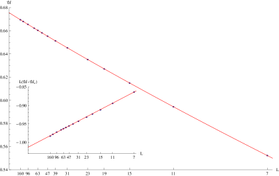
Figure 1: (Colour on-line) Mean energy $\mathcal{U}$ at $K_{c}$ versus $1/L$ for $L=7$, $11$, $15$, $19$, $23$, $31$, $39$, $47$, $55$, $63$, $72$, $96$, $128$ and $160$. The red curve is $0.675647-1.013\,x+0.395\,x^{3/2}$ where $x=1/L$. Error bars are too small to be seen. See text for details. The inset shows the scaled energy $L(\mathcal{U}-\mathcal{U}_{c})$ at $K_{c}$ versus $1/L^{1/2}$ for the same range of $L$. Error bars are too small to be seen. The red curve $-1.013+0.395\,x$.

For the specific heat we note that the error bars are noticeable, but this is to be expected. It is not known at which rate $\mathcal{C}(K_{c},L)$ approaches its asymptotic value $\mathcal{C}_{c}$ but judging from the excellent line-up of the points in Fig. 2 it appears $\mathcal{C}(K_{c},L)-\mathcal{C}_{c}\propto 1/L^{1/3}$. This is the only time we see a $1/3$ in a scaling exponent for free boundary conditions and we have no theoretical basis for it. In Fig. 2 we show $\mathcal{C}(K_{c},L)$ versus $1/L^{1/3}$ and the line $14.69(1)-14.93(2)x$, where $x=1/L^{1/3}$. As before the error estimates of the coefficients are based on the variability of a fitted curve after deleting one of the points. We estimate thus that $\mathcal{C}_{c}=\lim_{L\to\infty}\mathcal{C}(K_{c},L)=14.69(1)$. The inset picture of Fig. 2 zoom into the correction term by plotting $L^{1/3}(\mathcal{C}-\mathcal{C}_{c})$ versus $1/L^{1/3}$ together with the constant line $-14.93$. The error bars now become quite noticeable, especially for the larger $L$. There is no clear trend upwards or downwards in the data points which suggests that any further corrections to scaling must be truly negligible.

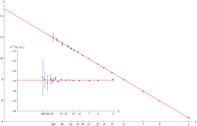
Figure 2: (Colour on-line) Specific heat $\mathcal{C}$ at $K_{c}$ versus $1/L^{1/3}$ for $L=3$, $5$, $7$, $11$, $15$, $19$, $23$, $31$, $39$, $47$, $55$, $63$, $72$, $96$, $128$ and $160$. The red line is $14.69-14.93\,x$ where $x=1/L^{1/3}$. The inset shows the scaled specific heat $L^{1/3}(\mathcal{C}-\mathcal{C}_{c})$ at $K_{c}$ versus $1/L^{1/3}$ for the same range of $L$. The red line is the constant $-14.93$.

IV Magnetisation and susceptibility

The scaling of the modulus of the magnetisation $\langle|m|\rangle$ for free boundary conditions is very different from that of periodic boundary conditions. In the first case we find $\langle|m|\rangle\propto L^{-3/2}$ whereas in the second it is well-known that $\langle|m|\rangle\propto L^{-5/4}$. In the free boundary case we note the need for correction to scaling. Indeed, if we want perfectly fitted curves down to $L=3$ we need two correction terms. We have instead chosen to ignore $L\leq 7$ and stay with just one correction term for the remaining $13$ points. In Fig. 3 we show $\langle|m|\rangle L^{3/2}$ versus $1/L$ for $11\leq L\leq 160$ together with the curve $0.22958(6)+1.101(3)\,x-1.63(3)\,x^{2}$. We test the fit of this curve by zooming into the picture and instead show $(\langle|m|\rangle L^{3/2}-0.22958)L$ which then should be well fitted by the line $1.101-1.63\,x$. As the inset of Fig 3 shows, it is and we conclude that to leading order $\langle|m|\rangle\sim 0.22958(6)L^{-3/2}$. However, the error bars for the largest systems are now quite pronounced.

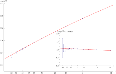
Figure 3: (Colour on-line) Modulus magnetisation $\langle|m|\rangle L^{3/2}$ at $K_{c}$ versus $1/L$ for $L=11$, $15$, $19$, $23$, $31$, $39$, $47$, $55$, $63$, $72$, $96$, $128$ and $160$. The red curve is $0.22958+1.101\,x-1.63\,x^{2}$, where $x=1/L$. The inset shows the scaled magnetisation $(\langle|m|\rangle L^{3/2}-0.22958)L$ at $K_{c}$ versus $1/L$ for the same range of $L$. The red line is $1.101-1.63\,x$.

As we mentioned above the susceptibility $\chi=N\langle m^{2}\rangle$ scales to leading order as $\chi\propto L^{5/2}$ for periodic boundary conditions but it is not known what the corresponding order is for free boundary conditions. We find here, as in Ref. Lundow and Markström (2011), that $\chi\propto L^{2}$ is by far the best scaling rule. In Fig. 4 we show $\chi/L^{2}$ versus $1/L$ for $7\leq L\leq 160$ together with the line $0.08269(2)+0.8174(3)\,x$. The coefficients were determined after excluding $L\leq 5$ from the fitting process. Had we included the two smallest systems an extra correction to scaling term would have been required. Again we zoom in and the inset of Fig. 4 shows $(\chi/L^{2}-0.08269)L$ versus $1/L$ together with the constant line $0.8174$. Though the error bars are quite big for the largest systems the fit is quite acceptable. In short we find $\chi(K_{c})\sim 0.08269(2)L^{2}$. We might add that the corresponding expression for periodic boundary is not known exactly but we suggested recently Lundow and Rosengren (2013) that $\chi\sim 1.742L^{5/2}$.

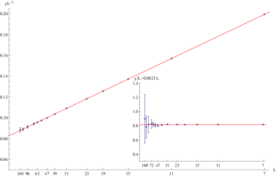
Figure 4: (Colour on-line) Normalised susceptibility $\chi/L^{2}$ at $K_{c}$ versus $1/L$ for $L=7$, $11$, $15$, $19$, $23$, $31$, $39$, $47$, $55$, $63$, $72$, $96$, $128$ and $160$. The red line is $0.08269+0.8174\,x$, where $x=1/L$. The inset shows the scaled and normalised susceptibility $(\chi/L^{2}-0.08269)L$ at $K_{c}$ versus $1/L$ for the same range of $L$. The red line is the constant $0.8174$.

V Susceptibility compared to $L^{5/2}$

It has been suggested Berche et al. (2012b) that $L^{2}$ is in fact not the correct scaling for the susceptibility. The authors of Berche et al. (2012b) claim that the correct scaling should be $L^{5/2}$, as for the case with cyclic boundary conditions, and that the exponent previously found by us, and other authors, are based on either finite size effects due to too many boundary vertices in small systems, for simulation studies, or incomplete theory. In our previous work the boundary did indeed contain a large fraction of the system’s vertices but in our current study this fraction has been reduced to a lower value than in any previous study, including the truncated systems used in Berche et al. (2012b).

To avoid implicit bias in our scaling of the susceptibility to we can also test the ratio $\chi/L^{5/2}$. If the claims of Berche et al. (2012b) are correct this quantity should converge to a finite non-zero limit, at least for large enough systems, and if the standard scaling is correct it should to leading order converge to 0 as $L^{-0.5}$. We make a scaling ansatz $c_{0}+c_{1}\,x^{\lambda_{1}}+c_{2}\,x^{\lambda_{2}}$, where $x=1/L$, and let Mathematica find the five free parameters using a least squares fit, after excluding $L=3,5$. As usual, we let each remaining point be deleted in turn from the fitting data to obtain error bars of the parameters. We find on average the curve $0.0000(4)+0.085(9)\,x^{0.51(3)}+0.820(7)\,x^{1.51(3)}$. Clearly the parameters we estimated above for $\chi/L^{2}$ falls inside these estimates, though the error bars are a magnitude larger here. Using the middle point values we plot the curve together with the data points in Fig. 5. The data for large systems is clearly consistent with the standard scaling, even for an unrestricted data fitting like this.

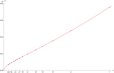
Figure 5: (Colour on-line) Normalised susceptibility $\chi/L^{5/2}$ at $K_{c}$ versus $1/L$ for $L=7$, $11$, $15$, $19$, $23$, $31$, $39$, $47$, $55$, $63$, $72$, $96$, $128$ and $160$. The red curve is $0.085\,x^{0.51}+0.82\,x^{1.51}$, where $x=1/L$.

VI Fourth moment and kurtosis

Our final property of interest is the fourth moment of the magnetisation at $K_{c}$. We find that the fourth moment of the magnetisation scales as $\langle m^{4}\rangle\propto L^{-6}$. The general rule would then be $\langle|m^{k}|\rangle\propto L^{-3k/2}$ whereas the corresponding rule for periodic boundary conditions is $\langle|m^{k}|\rangle\propto L^{-5k/4}$. Proceeding in the same manner as before, we plot the normalised fourth moment’s behaviour as $\langle m^{4}\rangle L^{6}$ versus $1/L$ in Fig. 6 together with the estimated polynomial $0.02051(3)+0.4045(8)\,x+1.989(4)\,x^{2}$. We excluded $L=3$ from the coefficient estimates. To leading order we thus find $\langle m^{4}\rangle\sim 0.02051(3)L^{-6}$.

The moment ratio $Q=\langle m^{4}\rangle/\langle m^{2}\rangle^{2}$, or kurtosis, indicates the shape of the underlying magnetisation distribution. In Fig. 7 we show the kurtosis versus $1/L$ and the line $3-0.14\,x$. The error bars are based on the formula for the error of a quotient, $\mathrm{d}(x/y^{2})$. The line is based on the coefficient estimates for $m^{2}$ and $m^{4}$ above by taking the quotient of their respective series expansions in the standard fashion. Inserting the coefficients and their error estimates gives the limit $\langle m^{4}\rangle/\langle m^{2}\rangle^{2}\to 3.000(6)$ which is the characteristic value of a gaussian distribution. Recall that for periodic boundary conditions the kurtosis at $K_{c}$ takes the asymptotic value $\Gamma(1/4)^{4}/2\pi^{2}=2.1884\ldots$, see Refs. Brezin and Zinn-Justin (1985); Lundow and Rosengren (2013)

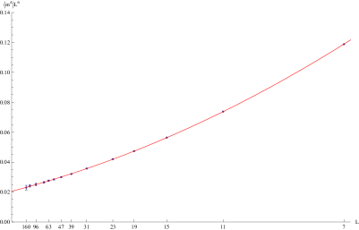
Figure 6: (Colour on-line) Normalised fourth moment $\langle m^{4}\rangle L^{6}$ at $K_{c}$ versus $1/L$ for $L=7$, $11$, $15$, $19$, $23$, $31$, $39$, $47$, $55$, $63$, $72$, $96$, $128$ and $160$. The red curve is $0.02051+0.4045\,x+1.989\,x^{2}$, where $x=1/L$.

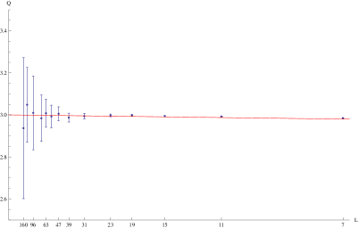
Figure 7: (Colour on-line) Kurtosis $\langle m^{4}\rangle/\langle m^{2}\rangle^{2}$ at $K_{c}$ versus $1/L$ for the same range of $L$ as in Fig. 6. The red line is $3-0.14\,x$, where $x=1/L$.

VII Kurtosis at an effective critical point

That the kurtosis takes the asymptotical value $3$ at $K_{c}$ does of course not mean that the kurtosis converges to $3$ for every sequence of temperatures $K_{c}(L)$ that has $K_{c}$ as limit. We exemplify this by reexamining some of our data used in Ref. Lundow and Markström (2011) where we relied on extremely detailed data on a wide temperature range for $4\leq L\leq 20$. For $L=4,6,8,10$ we also have magnetisation distributions. Let us say that $K_{c}(L)$ is the point where the variance of the modulus magnetisation, i.e. $\bar{\chi}=N\left(\left\langle m^{2}\right\rangle-\left\langle|m|\right\rangle^{2}\right)$, takes its maximum value. The distribution is here at its widest and on the threshold of breaking up into two parts, see Fig. 8 where we show a scaled distribution at $K_{c}(L)$ for $L=4,6,8,10$, in stark contrast to the distribution at $K_{c}$ of Fig. 9. Measuring the kurtosis at this point produces Fig. 10 which shows $Q(K_{c}(L),L)$ versus $1/L$ and a fitted 2nd degree polynomial which suggests the limit $1.520$. The absence of error bars is due to the method by which the original data were produced. However, we expect the error to be smaller than the plotted points. In fact, repeating this exercise for periodic boundary conditions suggests the limit $1.517$. There is a distinct possibility that these two limits are in fact the same, but that would require high-resolution data for larger systems to resolve than is at our disposal. In any case this subject falls outside the scope of this paper.

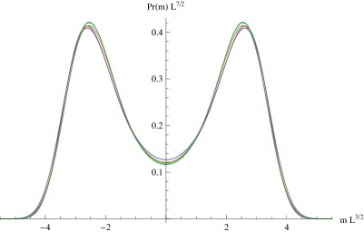
Figure 8: (Colour on-line) Scaled magnetisation distributions $\Pr(m)L^{7/2}$ versus $mL^{3/2}$ at $K_{c}(L)$ (see text) for $L=4$, $6$, $8$ and $10$.

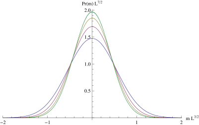
Figure 9: (Colour on-line) Scaled magnetisation distributions $\Pr(m)L^{7/2}$ versus $mL^{3/2}$ at $K_{c}$ for $L=4$, $6$, $8$ and $10$ (increasing at $y$-axis). Data from Ref. Lundow and Markström (2011).

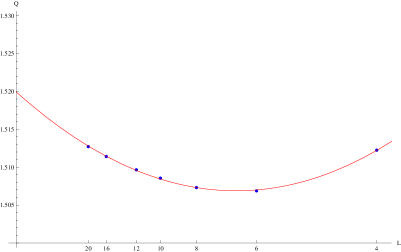
Figure 10: (Colour on-line) Kurtosis $Q=\langle m^{4}\rangle/\langle m^{2}\rangle^{2}$ at $K_{c}(L)$ (see text) versus $1/L$ for $L=4$, $6$, $8$, $10$, $12$, $16$, $20$. The red curve $1.52-0.17\,x+0.56\,x^{2}$, where $x=1/L$.

VIII Discussion and Conclusions

As we have seen the sampled data for cubes up to side $L=160$ agree well with the standard scaling picture for free boundary conditions, and e.g. recent long series expansions Butera and Pernici (2012) also appears to favour this version, nontheless without a rigorous bound for the rate of convergence a simulation study is always open to the claim that it is dominated by finite size effects.

However, the last decade has seen a number of rigorous mathematical results on the behaviour of the random-cluster model which leads us to believe that the standard scaling is indeed the right one. The Fortuin-Kasteleyn random-cluster model has a parameter $q$ which governs the properties of the model. We’ll refer the reader to Grimmett (2004) for more details and history. We recall that for $q=1$ the model is the standard bond percolation model, for $q=2$ it is equivalent to the Ising model, and in the limit $q\rightarrow 0$ we get the uniform random spanning tree, or the uniform spanning forest, depending on the parameter $p$.

For the random spanning tree on the $d$-dimensional lattice with different boundary conditions Pemantle Pemantle (1991) begun a study which related it to the loop erased random walk and demonstrated a strong dependency on both the dimension and boundary condition. In later papers Benjamini and Kozma (2005); Schweinsberg (2008, 2009) these results were refined to show, among other things, that for large enough $d$ that for two points in a grid with side $L$ and free boundary the distance between the two points within the tree scale as $L^{2}$, but that for the torus of side $L$ the distance scales as $L^{d/2}$.

Coming to the case $q=1$, Aizenman Aizenman (1997) studied the behaviour of the largest crossing clusters, i.e clusters which contain vertices on opposite sides of the box, in percolation on grids in different dimensions. Among other things he conjectured that at the critical point $p_{c}$, for all large enough dimensions $d$ the largest cluster in the case with free boundary should scale as $L^{4}$, and for the torus, or cyclic boundary, it should scale as $L^{2d/3}$. This conjecture was proven in Heydenreich and van der Hofstad (2007, 2011), and so we know that for percolation the boundary condition have a large and non-vanishing effect on the size of the largest clusters at the critical point. It is also important to point out that the results from Heydenreich and van der Hofstad (2007, 2011) are for the scaling exactly at the critical point $p_{c}$. For other sequences of points converging to $p_{c}$ different scaling behaviours can appear.

The reason for the drastic difference between the torus and free boundary case here is that for large $d$ the clusters in the model become much more spread out than in low dimensions. For $d=2$ clusters at $p_{c}$ are always finite and have a boundary which in the scaling limit is very close to a brownian motion Smirnov and Werner (2001). For a finite box of side $L$, with free boundary the number of crossing clusters, has a finite mean, bounded as $L$ grows, and the probability that there are more than $k$ such clusters is less than $\exp(-a_{1}k^{2})$, for some positive constant $a_{1}$ Aizenman (1997). For a box with free boundary in $d>6$, the critical dimension for $q=1$, the number of crossing clusters is at least $a_{2}L^{d-6}$, for some constant $a_{2}$ Aizenman (1997). Further, the largest cluster and a positive proportion of the crossing clusters have size proportional to $L^{4}$, independently of $d$. The clusters are here of much lower dimension relative to that of the lattice and much more tree like in their structure than for $d=2$. If we instead consider a torus with $d>6$ the large number of these more expanding clusters lead them to connect up with other clusters, which would have been separate in the free boundary case, and this merging leads to maximum clusters that are vastly larger than in the free boundary case.

The current authors expect a picture similar to that for $q=1$ to hold for the Ising case $q=2$ as well. Since the susceptibility in the Ising model is proportional to the average cluster size in the random-cluster model this leads to a prediction of $L^{2}$ as the correct scaling for the free boundary case and $L^{5/2}$ for cyclic boundaries, for $d=5$. This would also lead us to expect the largest clusters in the free boundary case to scale as $L^{2}$. For our small to medium sized systems we collected the size of the cluster containing the central vertex of our cubes, a property which was also considered in Berche et al. (2012b) for truncated systems.

In Fig. 11 we show the normalised mean cluster size $\langle S_{0}\rangle/L^{2}$ for $3\leq L\leq 55$ as used in Berche et al. (2012b), together with a linear function estimated to be $0.3505(2)+0.600(1)x$. The inset shows the zoomed-in version $\langle S_{0}\rangle L^{-5/4}-0.3505L^{3/4}$ versus $1/L$ which then should essentially take the constant value $0.600$, the red line. As we can see we have an excellent fit to the prediction that this cluster size should scale as $L^{2}$.

Aizenman’s prediction Aizenman (1997) of $L^{2d/3}$ as the correct scaling for percolation on the torus, for high $d$, came from a comparison with the Erdös-Renyi random graph on $N$ vertices, for which the largest connected component at the critical probability, scales as $N^{2/3}$. In Lundow and Markström we follow this analogy further by comparing the largest cluster for the random-cluster model on 5-dimensional tori with the detailed rigorous results on the random-cluster model for complete graphs from Luczak and Luczak (2006), and a good agreement is found.

To conclude, we find that both the data from our simulations and the current mathematical result for the random-cluster model gives good support for the standard scaling picture for the Ising model with free boundary conditions, as well as a framework predicting further properties for the case with cyclic boundary.

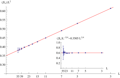
Figure 11: (Colour on-line) The normalised average size of the cluster containing the centre vertex, $\langle S_{0}\rangle/L^{2}$, plotted versus $1/L^{3/4}$ for $L=3$, $5$, $7$, $11$, $15$, $19$, $23$, $31$, $39$, $47$, $55$. The red line is $0.3505+0.600x$ where $x=1/L^{3/4}$. The inset shows the scaled and normalised cluster size $\langle S_{0}\rangle L^{-5/4}-0.3505L^{3/4}$ versus $1/L$. The red line is the constant $0.600$.

IX Acknowledgements

The simulations were performed on resources provided by the Swedish National Infrastructure for Computing (SNIC) at High Performance Computing Center North (HPC2N) and at Chalmers Centre for Computational Science and Engineering (C3SE).

References

- Aizenman (1982) M. Aizenman, Comm. Math. Phys. 86, 1 (1982), ISSN 0010-3616.
- Sokal (1979) A. D. Sokal, Phys. Lett. A 71, 451 (1979).
- Luijten et al. (1999) E. Luijten, K. Binder, and H. Blöte, Eur. Phys. J. B 9, 289 (1999).
- Binder (2008) K. Binder, Eur. Phys. J. B 64, 307 (2008), ISSN 1434-6028.
- Jones and Young (2005) J. L. Jones and A. P. Young, Phys. Rev. B 71, 174438 (2005).
- Berche et al. (2008) B. Berche, C. Chatelain, C. Dhall, R. Kenna, R. Low, and J.-C. Walter, J. Stat. Mech. 2008, P11010 (2008).
- Brezin and Zinn-Justin (1985) E. Brezin and J. Zinn-Justin, Nucl. Phys. B 257, 867 (1985).
- Lundow and Rosengren (2013) P. H. Lundow and A. Rosengren, Phil. Mag. 93, 1755 (2013).
- Chen and Dohm (2000) X. S. Chen and V. Dohm, Phys. Rev. E 63, 016113 (2000).
- Lundow and Markström (2011) P. H. Lundow and K. Markström, Nucl. Phys. B 845, 120 (2011).
- Berche et al. (2012a) B. Berche, R. Kenna, and J.-C. Walter, Nucl. Phys. B 865, 115 (2012a).
- Wolff (1989) U. Wolff, Phys. Rev. Lett 62, 361 (1989).
- Berche et al. (2012b) B. Berche, R. Kenna, and J.-C. Walter, Nucl. Phys. B 865, 115 (2012b).
- Butera and Pernici (2012) P. Butera and M. Pernici, Phys. Rev. E 85, 021105 (2012).
- Grimmett (2004) G. Grimmett, The random-cluster model (Springer, 2004).
- Pemantle (1991) R. Pemantle, Ann. Probab. 19, 1559 (1991).
- Benjamini and Kozma (2005) I. Benjamini and G. Kozma, Comm. Math. Phys. 259, 257 (2005).
- Schweinsberg (2008) J. Schweinsberg, J. Theoret. Probab. 21, 378 (2008).
- Schweinsberg (2009) J. Schweinsberg, Probab. Theory Related Fields 144, 319 (2009).
- Aizenman (1997) M. Aizenman, Nucl. Phys. B 485, 551 (1997).
- Heydenreich and van der Hofstad (2007) M. Heydenreich and R. van der Hofstad, Comm. Math. Phys. 270, 335 (2007).
- Heydenreich and van der Hofstad (2011) M. Heydenreich and R. van der Hofstad, Probab. Theory Related Fields 149, 397 (2011).
- Smirnov and Werner (2001) S. Smirnov and W. Werner, Math. Res. Lett. 8, 729 (2001).
- (24) P. H. Lundow and K. Markström, arXiv:1408.2155.
- Luczak and Luczak (2006) M. J. Luczak and T. Luczak, Random Struct. Algorithms 28, 215 (2006).