High Performance Financial Simulation Using Randomized Quasi-Monte Carlo Methods

Abstract

GPU computing has become popular in computational finance and many financial institutions are moving their CPU based applications to the GPU platform. Since most Monte Carlo algorithms are embarrassingly parallel, they benefit greatly from parallel implementations, and consequently Monte Carlo has become a focal point in GPU computing. GPU speed-up examples reported in the literature often involve Monte Carlo algorithms, and there are software tools commercially available that help migrate Monte Carlo financial pricing models to GPU.

We present a survey of Monte Carlo and randomized quasi-Monte Carlo methods, and discuss existing (quasi) Monte Carlo sequences in GPU libraries. We discuss specific features of GPU architecture relevant for developing efficient (quasi) Monte Carlo methods. We introduce a recent randomized quasi-Monte Carlo method, and compare it with some of the existing implementations on GPU, when they are used in pricing caplets in the LIBOR market model and mortgage backed securities.

1 Introduction

The recent trend towards parallel computing in the financial industry is not surprising. As the complexity of models used in the industry grows, while the demand for fast, sometimes real-time, solutions persists, parallel computing is a resource that is hard to ignore. In 2009, Bloomberg and NVIDIA worked together to run a two-factor model for calculating hard-to-price asset-backed securities on 48 Linux servers paired with Graphics Processing Units (GPUs), which traditionally required about 1000 servers to accommodate customer demand. GPU computing offers several advantages over traditional parallel computing on clusters of CPUs. Clusters consume non negligible energy and space, and computations over clusters are not always easy to scale. In contrast, GPU is small, fast, and consumes only a tiny fraction of energy consumed by clusters. Consequently, there has been a recent surge in academic papers and industry reports that document benefits of GPU computing in financial problems. Arguably, the numerical method that benefits most from GPUs is the Monte Carlo simulation. Monte Carlo methods are inherently parallel, and thus more suitable for implementing on GPU than most alternative methods. In this paper we concentrate on Monte Carlo methods and financial simulation, and discuss computational and algorithmic issues when financial simulation algorithms are developed over GPU and traditional clusters.

The computational framework we use is the estimation of an integral $I=\int_{(0,1)^{s}}f(x)dx$ over the $s$ dimensional unit cube, using sums of the form $\theta_{N}=\frac{1}{N}\sum_{i=1}^{N}f(x_{i}).$ In Monte Carlo and quasi-Monte Carlo, $\theta_{N}$ converges to $I$ as $N\rightarrow\infty.$ In the former the convergence is probabilistic and $x_{i}$ come from a pseudorandom sequence, and in the latter the convergence is deterministic and the $x_{i}$ come from a low-discrepancy sequence. For a comprehensive survey of Monte Carlo and quasi-Monte Carlo methods, see Niederreiter (1992). Often it is desirable to obtain multiple independent estimates for $\theta,$ say $\theta^{1},...,\theta^{m},$ so that one could use statistics to measure the accuracy of the estimation by the use of sample standard deviation, or confidence intervals. Let us assume that an allocation of computing resources is done and we choose parameters $N,M$: the first parameter, $N,$ is the sample size, and gives the number of vectors from the sequence (pseudorandom or low discrepancy) to use in estimating $\theta:=\theta_{N}^{m}$

$$\theta_{N}^{m}=\frac{1}{N}\sum_{i=1}^{N}f(q_{i}^{m})$$

and the parameter $M$ gives the number of independent replications we obtain for $\theta_{N}$, i.e., $\theta_{N}^{1},...,\theta_{N}^{M}.$ The grand average $RQ_{M,N}$ gives the overall point estimate for $I:$

$$RQ_{M,N}=\frac{1}{M}\sum_{m=1}^{M}\theta_{N}^{m}.$$

In Monte Carlo, to obtain the independent estimates $\theta_{N}^{1},...,\theta_{N}^{M},$ one simply uses blocks of $N$ pseudorandom numbers. In quasi-Monte Carlo, one has to use methods that enable independent randomizations of the underlying low-discrepancy sequence. These methods are called randomized quasi-Monte Carlo (RQMC) methods (see Ökten and Eastman (2004), Ökten (2009)).

Traditionally, in parallel implementations of Monte Carlo algorithms, one often assigns the $m$th processor (of the $M$ allocated processors) the evaluation of the estimate $\theta_{N}^{m}.$ To do this computation, each processor needs to have an assigned number sequence (pseudorandom or low-discrepancy) and methods like blocking, leap-frogging, and parameterization are used to make this assignment. Parameterization is particularly useful when independent replications are needed to compute $RQ_{M,N}$ (see Ökten and Willyard (2010), and also deDoncker et al. (2000), Hofbauer et al. (2007), Ökten and Srinivasan (2002)). If only a single estimate is needed, then blocking or leap-frogging can be used (Bromley (1996), Chen et al. (2006), Li and Mullen (2000), Schmid and Uhl (1999), Schmid and Uhl (2001)). Figure 1(a) describes this traditional Monte Carlo implementation where the $m$th processor $p_{m}$ generates its assigned sequence $q_{1}^{m},...,q_{N}^{m}$ to compute $\theta_{N}^{m},$ as $m=1,...,M$. In many applications $N$ is typically in millions, and $M$ is large enough for statistical accuracy, in the range 50 to 100.

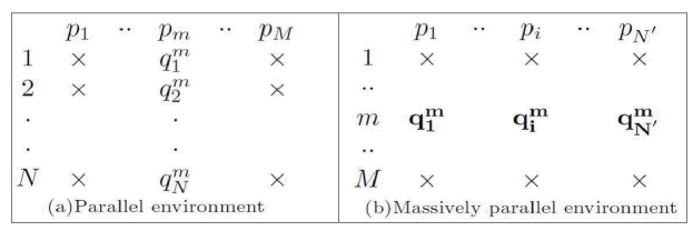
Figure 1: Different parallel computing strategies

In a massively parallel environment, depicted by the second diagram, where the number of processors $N^{{}^{\prime}}$is much larger than $M$, it can be a lot more efficient to completely “transpose” our computing strategy. Now the processors $p_{1},...,p_{N^{{}^{\prime}}}$ run simultaneously (for a total of $M$ times) to generate the sequence $\mathbf{q_{1}^{m}},\cdots,\mathbf{q_{N^{{}^{\prime}}}^{m}}$ to compute $\theta_{N}^{m},$ as $m=1,...,M$, where $\mathbf{q_{i}^{m}}$ is part of the sequence $\{q_{i}^{m},q_{N^{{}^{\prime}}+i}^{m},q_{2N^{{}^{\prime}}+i}^{m},...\}$ which is assigned to the $i$th processor.

The choice of the two computing paradigms, which we vaguely name as “parallel” and “massively parallel”, determines how the underlying sequence (pseudorandom or low-discrepancy) should be generated. In the parallel paradigm, a recursive algorithm for generating the underlying sequence works best since each processor generates the “entire” sequence. This paradigm is appropriate for a computing system with distributed memory, such as a cluster. For the massively parallel paradigm, a direct algorithm that generates the $n$th term of the sequence from $n$ is more appropriate. Salmon et al. (2011) use the term “counter-based” to describe such direct algorithms. The massively parallel paradigm is an appropriate model for GPU computing where prohibitive cost of memory access makes recursive computing inefficient.

In Section 2 we briefly discuss a counter-based pseudorandom number generator, called Philox, introduced by Salmon et al. (2011), and the pseudorandom number generators, Mersenne twister, and XORWOW. In Section 3 we introduce a randomized quasi-Monte Carlo sequence, which we name Rasrap, and give algorithms for recursive and counter-based implementations of this sequence. In this section, we also give a brief description of a well-known quasi-Monte Carlo sequence, the Sobol’ sequence. We will compare the computational time for generating these sequences on CPU and GPU, in Section 4.

2 Monte Carlo sequences

Most pseudorandom number generators are inherently iterative: they are generated by successive application of a transformation $F$ to an element of the state space to obtain the next element of the state space, i.e., $s_{n}=F(s_{n-1})$. Here we discuss some of the pseudorandom number generators considered in this paper. One of the most popular and high quality pseudorandom number generators is the Mersenne twister introduced by Matsumoto and Nishimura (1998). It has a very large period and excellent uniformity properties. It is available in many platforms, and recently Matlab adopted it as its default random number generator.

A parallel implementation of the Mersenne twister was also given by Matsumoto and Nishimura (1998). Their approach uses parameterization, and it falls under our parallel computing paradigm: each processor in the parallel environment generates a Mersenne twister, and different Mersenne twisters generated across different processors are assumed to be statistically independent. There are several parameters that need to be precomputed and stored to run the parallel implementation of Mersenne twister.

XORWOW is a fast pseudorandom number generator introduced by Marsaglia (2003). This generator is available in CURAND: a library for pseudorandom and quasi-random number generators for GPU provided by NVIDIA. However, the generator fails certain statistical tests; see Saito and Matsumoto (2012) for a discussion. The reason we consider this generator is because of its availability in CURAND, and that its computational speed can be used as a benchmark against which other generators can be compared.

Philox is a counter-based pseudorandom number generator introduced by Salmon et al. (2011). Its generation is in the form $s_{n}=F(n)$, and thus falls under our massively parallel computing paradigm. A comparison of some counter-based and conventional pseudorandom number generators (including Philox and Mersenne twister) is given in Salmon et al. (2011). In Section 4, we will present timing results comparing the pseudorandom number generators, and in Section 5 and 6, we will compare these sequences when they are used in some financial problems. These numerical results will also include Rasrap and Sobol’, two randomized-quasi Monte Carlo sequences that we discuss next.

3 Randomized-quasi Monte Carlo sequences

3.1 Rasrap

The van der Corput sequence, and its generalization to higher dimensions, the Halton sequence, are among the best well-known low-discrepancy sequences. The $n$th term of the van der Corput sequence in base $b$, $\phi_{b}(n)$, is defined as

$$\phi_{b}(n)=(.a_{0}a_{1}\cdots a_{k})_{b}=\frac{a_{0}}{b}+\frac{a_{1}}{b^{2}}+\cdots+\frac{a_{k}}{b^{k+1}},$$ (1)

where

$$n=(a_{k}\cdots a_{1}a_{0})_{b}=a_{0}+a_{1}b+\cdots+a_{k}b^{k}.$$ (2)

The Halton sequence in the bases $b_{1},\cdots,b_{s}$ is $(\phi_{b_{1}}(n),\cdots,\phi_{b_{s}}(n))_{n=0}^{\infty}$. This is a low-discrepancy sequence if the bases are relatively prime. In practice, $b_{i}$ is usually chosen as the $i$th prime number.

There is a well-known defect of the Halton sequence: in higher dimensions, when the base is larger, certain components of the sequence exhibit very poor uniformity. This is often referred to as high correlation between large bases. As a remedy, permuted (or, scrambled) Halton sequences were introduced. The permuted van der Corput sequence generalizes (1) as

$$\phi_{b}(n)=\frac{\sigma(a_{0})}{b}+\frac{\sigma(a_{1})}{b^{2}}+\cdots+\frac{\sigma(a_{k})}{b^{k+1}},$$ (3)

where $\sigma$ is a permutation on the digit set $\{0,\cdots,b-1\}$. By using different permutations for each base, one can define the permuted Halton sequences in the usual way. There are many choices for permutations published in the literature; a recent survey is given by Vandewoestyne and Cools (2006). In this paper, we will follow the approach used in Ökten et al. (2012) and pick these permutations at random.

The Halton sequence can be generated recursively, which would be appropriate for an implementation on CPU, or directly (counter-based), which would be appropriate for GPU. Next we discuss some recursive and counter-based algorithms for the Halton sequence.

A fast recursive method for generating the van der Corput sequence was given by Struckmeier (1993). We now explain his algorithm. Let $p$ be a positive integer and $x\in[0,1)$ arbitrary. Define the sequence $(b_{k}^{p})_{k\in\mathbb{N}}$ by

$$b_{k}^{p}=\frac{1}{p^{k}}(p+1-p^{k})\;\forall k\in\mathbb{N},$$ (4)

and the transformation $T_{p}$ by

$$T_{p}(x)=x+b_{k}^{p},$$ (5)

where

$$k=\left\lfloor-\frac{\ln(1-x)}{\ln p}\right\rfloor+1.$$ (6)

The transformation $T_{p}$ is called the von Neumann - Kakutani transformation in base $p.$ The orbit of zero under $T_{p},$ i.e., $\{0,T_{p}(0),T_{p}^{2}(0),...\}$ is the van der Corput sequence in base $p$. In fact, the orbit of any point $x_{0}\in[0,1)$ under $T_{p}$ is a low-discrepancy sequence. If $x_{0}$ is chosen at random from the uniform distribution on $[0,1),$ then the orbit of $x_{0}$ under $T_{p}$ is called a random-start van der Corput sequence in base $p.$ The following algorithm summarizes the construction by Struckmeier (1993) of the (random-start) van der Corput sequence in base $p.$ It can be generalized to Halton sequences in the obvious way.

Struckmeier (1993). Generates a random-start van der Corput sequence with starting point $x_{0}$ and base $p.$

1. Generate the sequence $b_{k}^{p}$ according to (4);

2. Choose an arbitrary starting point $x\in[0,1)$;

3. Calculate $k$ according to (6);

4. $x=x+b_{k}^{p}$;

5. Repeat step 3-4.

Algorithm 3.1 is prone to rounding error in floating number operations due to the floor operation in (6). For example, a C++ compiler gives a wrong index $k$ after 3 steps of iteration when the starting point is $x=0$ if the rounding error introduced in (4) is not carefully handled.

We now suggest an alternative algorithm that computes a random-start permuted Halton sequence. The advantages of this algorithm over Algorithm 3.1 are: (i) it avoids rounding errors, (ii) it is faster, and (iii) it can be used to generate permuted Halton sequences.

(Recursive) Generates a random-start permuted van der Corput sequence in base $p$.

1. Initialization Step. Generate a random number $\omega\in[0,1)$ and find some integer $n$ so that $\omega$ is the $n^{th}$ term in the van Corput sequence in base $p$. Initialize and store a random digit permutation $\sigma$. Expand $n$ in base $p$ as $n=(a_{k}\cdots a_{1}a_{0})_{p}$ ($k$ depends on $n$). Set $a_{i}=0$ for $i>k$. Store $a_{k},\cdots,a_{1},a_{0}$. Calculate and store $S_{j}=\sum_{i=j}^{k}\frac{\sigma(a_{i})}{p^{i+1}}$ for $j=k,k-1,\cdots,1,0$. Set $S_{j}=0$ for $j>k$. Set the quasi-random number $r=S_{0}$;

2. Let $n=n+1$. Find $\min\{m|a_{m}+1<p\}$;

3. $S_{m}=S_{m+1}+\frac{\sigma(a_{m}+1)}{p^{m+1}}$. Set $a_{m}=a_{m}+1$. Set $a_{i}=0,S_{i}=S_{i+1}+\frac{\sigma(0)}{p^{i+1}}$ for $i=m-1,m-2,\cdots,1,0$. The quasi-random number corresponding to $n+1$ is $r=S_{0}$;

4. Repeat step 2-3.

Algorithm 2 is an efficient iterative algorithm appropriate for the parallel computing paradigm. However, for the massively parallel computing paradigm, such as GPU computing, we need a counter-based algorithm. For the Halton sequence, this would be simply its definition:

(Counter-based) Generates a random-start permuted van der Corput sequence in base $p$.

1. Initialization step: Choose a small positive real number, $\epsilon$. Generate a random number $\omega$ from the uniform distribution on $(0,1)$, and find $n$ such that $|\phi_{p}(n)-\omega|<\epsilon$;

2. The quasi-random number corresponding to $n$ is $\phi_{p}(n)$;

3. Let $n=n+1$ and repeat step 2-3.

The name Rasrap is an abbreviation for random-start randomly permuted Halton sequence: if in Algorithms 3.1 and 3.1, the permutations for each base are generated at random, then we obtain Rasrap.

3.2 Sobol’ sequence

The Sobol’ sequence is a well-known fast low-discrepancy sequence popular among financial engineers. The $j$th component of the $i$th vector in a Sobol’ sequence is calculated by

$x_{i}^{j}=i_{1}v_{1}^{j}\oplus i_{2}v_{2}^{j}\oplus\cdots$,

where $i_{k}$ is the $k$th digit from the right when integer $i$ is represented in base $2$ and $\oplus$ is the bitwise exclusive-or operator. The so-called direction numbers, $v_{k}^{j}$, are defined as

$v_{k}^{j}=\frac{m_{k}^{j}}{2^{k}}.$

To generate the Sobol’ sequence, we need to generate a sequence of positive integers $\{m_{k}^{j}\}$. The sequence $\{m_{k}^{j}\}$ is defined recursively as follows:

$m_{k}^{j}=2a_{1}^{j}m_{k-1}^{j}\oplus 2^{2}a_{2}^{j}m_{k-2}^{j}\oplus\cdots\oplus 2^{s_{j}-1}a_{s_{j}-1}^{j}m_{k-s_{j}+1}^{j}\oplus 2^{s_{j}}m_{k-s_{j}}^{j}\oplus m_{k-s_{j}}^{j}$,

where $a_{1}^{j},a_{2}^{j},\cdots,a_{s_{j}-1}^{j}$ are coefficients of a primitive polynomial of degree $s_{j}$ in the field $\mathbb{Z}_{2}$,

$x^{s_{j}}+a_{1}^{j}x^{s_{j}-1}+a_{2}^{j}x^{s_{j}-2}+\cdots+a_{s_{j}-1}^{j}x+1$.

The initial values $m_{1}^{j},m_{2}^{j},\cdots,m_{s_{j}}^{j}$ can be chosen freely given that each $m_{l}^{j},1\leq l\leq s_{j}$, is odd and less than $2^{l}$. Because of this freedom, different choices for direction numbers can be made based on different search criteria minimizing the discrepancy of the sequence. We use the primitive polynomials and direction numbers provided by Joe and Kuo (2008).

The counter-based implementation of the Sobol’ sequence introduced here is convenient on GPUs, but a more efficient implementation proposed by Antonov and Saleev based on Gray code is used in practice on CPUs. For details about this approach, see Antonov and Saleev (1979).

The Sobol’ sequence can be randomized using various randomized quasi-Monte Carlo methods. Here we will use the random digit scrambling method of Matoušek (1998). More on randomized quasi-Monte Carlo and some parallel implementations can be found in Ökten and Eastman (2004), and, Ökten and Willyard (2010).

4 Performance Comparison

Mersenne twister, Philox, XORWOW, Rasrap, and Sobol’ sequences are run on Intel i7 3770K and NVIDIA GeForce GTX 670. We compare the throughput of different algorithms on CPU (Table 1) and GPU (Table 2).

Table 1 shows that the fastest algorithm for the Halton sequence on CPU is Algorithm 2. It is about 3.8 times as fast as the algorithm by Struckmeier (Algorithm 1). Not surprisingly Algorithm 3, the counter-based implementation, is considerably slower on CPU. Mersenne twister uses its serial CPU implementation and it is about 3.4 times faster than Algorithm 2 for the Halton sequence. And Sobol’ sequence based on Gray code is faster than Mersenne twister.

Table 2 shows that the throughput of Algorithm 3 on GPU improves significantly compared to the CPU value. Counter-based Sobol’ sequence is twice as fast as Rasrap, and the pseudorandom number generator Philox is almost 200 times faster than Rasrap.

Throughput of generators on CPU. Throughput (GNumbers/s) Twister 0.598 Rasrap Algo. 3.1 0.045 Rasrap Algo. 3.1 0.173 Rasrap Algo. 3.1 0.012 Sobol’(Counter based) 0.04 Sobol’(Gray Code) 0.97

Throughput of generators on GPU. Throughput (GNumbers/s) XORWOW 60 Philox 190 Rasrap Algo. 3.1 1.0 Sobol’(Counter based) 2.0

The computational speed at which various sequences are generated is only one part of the story. We next examine the accuracy of the estimates obtained when these sequences are used in simulation. In the next section, we use these sequences in two problems from computational finance, and compare them with respect to the standard deviation of their estimates and computational speed.

5 Pricing caplets in the LIBOR model

An interest rate derivative is a derivative where the underlying asset is the right to pay or receive a notional amount of money at a given interest rate. The interest rate derivatives market is the largest derivatives market in the world. To price interest rate derivatives, forward interest rate models are widely used in the industry. There are two kinds of forward rate models: the continuous rate model and the simple rate model.

The framework developed by Heath et al. (1992) (HJM) explicitly describes the dynamics of the term structure of the interest rates through the dynamics of the forward rate curve. HJM model has two major drawbacks: (1) the instantaneous forward rates are not directly observable in the market; (2) some simple choices of the form of volatility is not admissible.

In practice, many fixed income securities quote the interest rate on an annual basis with semi-annual or quarterly compounding, instead of a continuously compounded rate. The simple forward rate models describe the dynamics of the term structure of interest rates through simple forward rates, which are observable in the market. This approach is developed by Miltersen et al. (1997), Brace et al. (1997), Musiela and Rutkowski (1997) and Jamshidian (1997).

The London Inter-Bank Offered Rates (LIBOR) is one of the most important benchmark simple interest rates. Let $B(t,T)$ denote the time-$t$ value of a zero coupon bond paying 1 at the maturity time $T$. A forward rate $F(t,T_{1},T_{2})$ ($t<T_{1}<T_{2}$ ) is an interest rate fixed at time $t$ for borrowing or lending at time $T_{1}$ over the period $[T_{1},T_{2}]$. An arbitrage argument shows that forward rates are determined by bond prices in accordance to

$$F(t,T_{1},T_{2})=\frac{1}{T_{2}-T_{1}}\bigg{(}\frac{B(t,T_{1})-B(t,T_{2})}{B(t,T_{2})}\bigg{)}.$$ (7)

A forward LIBOR rate is a special case of (7) with a fixed period $\delta=T_{2}-T_{1}$ for the accrual period. Typically $\delta=0.5$ or $0.25$. Thus, the $\delta$-year forward LIBOR rate at time $t$ with maturity $T$ is

$$L(t,T)=F(t,T,T+\delta)=\frac{1}{\delta}\bigg{(}\frac{B(t,T)-B(t,T+\delta)}{B(t,T+\delta)}\bigg{)}.$$ (8)

So if we enter into a contract at time $0$ to borrow 1 at time $T$ and repay it with interest at time $T+\delta$, the interest due will be $\delta L(0,T)$.

Fix a finite set of maturities

$0=T_{0}<T_{1}<\cdots<T_{M}<T_{M+1}$

and let

$\delta_{i}=T_{i+1}-T_{i},\;i=0,\cdots,M$,

denote the lengths of the intervals between maturities. Normally we fix $\delta$ as a constant regardless of day-count conventions that would introduce slightly different values for the fractions $\delta_{i}$.

For each maturity $T_{n}$, let $B_{n}(t)$ denote the time-$t$ value of a zero coupon bond maturing at $T_{n},\;0\leq t\leq T_{n}$. And write $L_{n}(t)$ for the forward rate at time $t$ over the period $[T_{n},T_{n+1}]$. Equation (8) can be then rewritten as

$$L_{n}(t)=\frac{B_{n}(t)-B_{n+1}(t)}{\delta_{n}B_{n+1}(t)},\;0\leq t\leq T_{n},\;n=0,1,\cdots,M.$$ (9)

The subscript $n=0,1,\cdots,M$ emphasizes we are looking at a finite set of bonds.

The dynamics of the forward LIBOR rates can be described as a system of SDEs as follows. For a brief informal derivation, see Glasserman (2003).

$$\frac{dL_{n}(t)}{L_{n}(t)}=\sum_{j=\eta(t)}^{n}\frac{\delta_{j}(t)L_{j}(t)\sigma_{n}(t)^{\top}\sigma_{j}(t)}{1+\delta_{j}L_{j}(t)}dt+\sigma_{n}(t)^{\top}dW(t),\;0\leq t\leq T_{n},\;n=1,\cdots,M.$$ (10)

where $W$ is a $d$-dimensional standard Brownian motion and the volatility $\sigma_{n}$ may depend on the current vector of rates $(L_{1}(t),\cdots,L_{M}(t))$ as well as the current time $t$. $\eta(t)$ is the unique integer such that $T_{\eta(t)-1}\leq t<T_{\eta(t)}$.

Pricing interest rate derivative securities with LIBOR market models normally requires simulations. Since the LIBOR market model deals with a finite number of maturities, only the time variable needs to be discretized.

We fix a time grid $0=t_{0}<t_{1}<\cdots<t_{m}<t_{m+1}$ to simulate the LIBOR market model. In practice, one would often take $t_{i}=T_{i}$ so the simulation goes directly from one maturity date to the next. For simplicity, we use a constant volatility $\sigma$ in the simulation. We apply an Euler scheme to (10) to discretize the system of SDEs of the LIBOR market model, producing

$$\hat{L}_{n}(t_{i+1})=\hat{L}_{n}(t_{i})+\mu_{n}(\hat{L}(t_{i}),t_{i})\hat{L}_{n}(t_{i})[t_{i+1}-t_{i}]+\hat{L}_{n}(t_{i})\sqrt{t_{i+1}-t_{i}}\sigma_{n}(t_{i})^{\top}Z_{i+1},$$ (11)

where

$$\mu_{n}(\hat{L}(t_{i}),t_{i})=\sum_{j=\eta(t_{i})}^{n}\frac{\delta_{j}\hat{L}_{j}(t_{i})\sigma_{n}(t_{i})^{\top}\sigma_{j}(t_{i})}{1+\delta_{j}\hat{L}_{j}(t_{i})}$$ (12)

and $Z_{1},Z_{2},\cdots$ are independent $N(0,I)$ random vectors in $\mathbb{R}^{d}$. Here hats are used to identify discretized variables.

We assume an initial set of bond prices $B_{1}(0),\cdots,B_{M+1}(0)$ is given and initialize the simulation by setting

$$\hat{L}_{n}(0)=\frac{B_{n}(0)-B_{n+1}(0)}{\delta_{n}B_{n+1}(0)},\;n=1,\cdots,M,$$ (13)

in accordance with (9).

Next we use the simulated evolution of LIBOR market rates to price a caplet. An interest rate cap is a portfolio of options that serve to limit the interest paid on a floating rate liability over a set of consecutive periods. Each individual option in the cap applies to a single period and is called a caplet. It is sufficient to price caplets since the value of a cap is simply the sum of the values of its component caplets.

We follow the derivation in Glasserman (2003). Consider a caplet for the time period $[T,T+\delta]$. A party with a floating rate liability over that period would pay interest $\delta L(T,T)$ times the principle at time $T+\delta$. A caplet is designed to limit the interest paid to a fixed level $K$. The difference $\delta(L(T,T)-K)$ would be refunded only if it is positive. So the payoff function of a caplet is

$\delta(L(T,T)-K)^{+}$,

where the notation $(\cdot)^{+}$ indicates that we take the maximum of the expression in parentheses and zero. This payoff is exercised at time $T+\delta$ but determined at time $T$. There is no uncertainty in the payoff over the period $[T,T+\delta]$. Then the payoff function at time $T+\delta$ is equal to

$$\frac{\delta(L(T,T)-K)^{+}}{1+\delta L(T,T)}=\delta B(T,T+\delta)(L(T,T)-K)^{+}$$ (14)

at time $T$. This payoff typically requires the simulation of the dynamics of the term structure.

Black (1976) derived a formula for the time-$t$ price of the caplet under the assumption of $L_{n}(T_{n})$ following a lognormal distribution, which does not necessarily correspond to a price in the sense of the theory of derivatives valuation. In practice, this formula

$$\sigma B(t,T+\delta)\Bigg{(}L(t,T)\Phi\bigg{(}\frac{\log(L(t,T)/K)+\sigma^{2}(T-t)/2}{\sigma\sqrt{T-t}}\bigg{)}$$

$$-K\Phi\bigg{(}\frac{\log(L(t,T)/K)-\sigma^{2}(T-t)/2}{\sigma\sqrt{T-t}}\bigg{)}\Bigg{)}$$ (15)

is used to calculate the “implied volatility” $\sigma$ from the market price of caps.

To test the correctness of the LIBOR market model simulation, we use the daily treasury yield curve rates on 02/24/2012 as shown in Table 3 to initialize the LIBOR market rates simulation. We first apply a cubic spline interpolation to the rates in Table 3 to get estimated yield curve rates for every 6 months. Then the estimated yield curve rates are used to calculate the bond prices for every 6 months in order to initialize the LIBOR rates in (13). We assume the following parameters in LIBOR rates simulation

$(t,T,\delta,K,\sigma)=(0,5,0.5,0.01,0.04).$

The daily Treasury yield curve rates on 02/24/2012. Date 1 mo 3 mo 6 mo 1 yr 2 yr 3 yr 5 yr 7 yr 10 yr 20 yr 30 yr 02/24/2012 0.08 0.10 0.14 0.18 0.31 0.43 0.89 1.41 1.98 2.75 3.10

The simulations are run on Intel i7 3770K and NVIDIA GeForce GTX 670 respectively. For a fixed sample size $N$, we repeat the simulation 100 times using independent realizations of the underlying sequence. We investigate the sample standard deviation of the 100 estimates and computing time as a function of the sample size $N$. We also compare the efficiency of different sequences, where efficiency is defined as the product of sample standard deviation and execution time.

5.1 Comparison of Sobol’ sequence implementations

The Sobol’ sequence and a scrambled version of it are provided in the CURAND library from NVIDIA. We use both the single precision version (Sobol’-lib(Single)) and double precision version (Sobol’-lib(Double)) in our simulation. We also implement our own version of the Sobol’ sequence (Sobol’(Single) and Sobol’(Double)) for comparison. Figure 2 plots the sample standard deviation of 100 estimates for the caplet price, computing time, and efficiency, of different implementations of the Sobol’ sequence against the sample size $N$. We also include the numerical results obtained using the fast pseudorandom number sequence XORWOW from CURAND as a reference. We make the following observations:

1. The convergence rate exhibits a strange behavior and levels off for the CURAND Sobol’ sequence generators, Sobol’-Lib(Single) and Sobol’-Lib(Double), as $N$ gets large. Our implementation of the Sobol’ sequence gives monotonically decreasing sample standard deviation as $N$ increases;

2. The execution time for CURAND generators Sobol’-Lib(Single) and Sobol’-Lib(Double) is significantly longer than our implementation, and not monotonic for a specific range of $N$;

3. The efficiency of CURAND generators Sobol’-Lib(Single) and Sobol’-Lib(Double) is even worse than the efficiency of the pseudorandom number sequence XORWOW. Our Sobol’ sequence implementations have better efficiency than XORWOW.

Due to the poor behavior of the Sobol’ sequence in the CURAND library, we will use our implementation of the Sobol’ sequence with single precision in the rest of the paper. We will denote this sequence simply as “Sobol’” in the numerical results.

5.2 Performance of Rasrap and Sobol’ on CPU

In Section 4, we compared the computing times of several sequences. Here we compare the performance of Mersenne twister, Rasrap and Sobol’, when they are used in simulating the LIBOR market model. The sequences are run on one CPU core.

Figure 3 shows that the sample standard deviation of the estimates obtained from Rasrap and Sobol’ sequences converge at a much faster rate than the Mersenne twister. The convergence rate for Mersenne twister is about $O(N^{-0.50})$, and the rate for Rasrap and Sobol’ is about $O(N^{-0.87})$ and $O(N^{-0.93})$, respectively.

The recursive implementation of Rasrap does not introduce much overhead in running time and gives very close timing results to Mersenne twister. The Sobol’ sequence based on Gray code is faster than Mersenne twister. As a result, the two low-discrepancy sequences enjoy better and “flatter” efficiency than that of Mersenne twister.

We next investigate how well Rasrap and Sobol’ sequence results scale over multi-core CPU. We implement a parallel version of Rasrap and Sobol’ with OpenMP that can run on 8 CPU cores simultaneously. Figure 4 plots the performance of OpenMP version of Rasrap and Sobol’ on CPU. It exhibits the same pattern of convergence, running time, and efficiency as in Figure 3. The convergence remains the same as in the one core case, but we gain a speedup of four with the parallelism using OpenMP.

5.3 Performance of GPU

In this section we compare the counter-based implementations of Rasrap and Sobol’ with pseudorandom sequences Philox and XORWOW, on GPU.

Figure 5 plots the sample standard deviation, computing time, and effciency. We make the following observations:

1. The convergence rate for Philox and XORWOW is about $O(N^{-0.52})$ and $O(N^{-0.51})$, respectively;

2. The convergence rate for Rasrap and Sobol’ is about $O(N^{-0.86})$ and $O(N^{-0.95})$ respectively;

3. XORWOW is the fastest generator, followed by Philox and Sobol’. Rasrap is slightly slower than Sobol’;

4. The efficiency of Sobol’ is the best among all sequences.

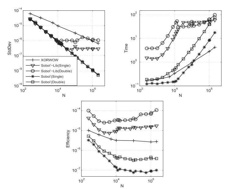
Figure 2: Comparing CURAND Sobol’ function with our implementation in pricing caplets

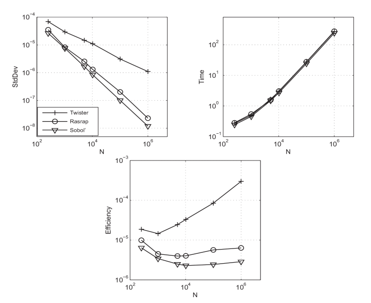
Figure 3: Comparing Mersenne twister, Rasrap, and Sobol’, when pricing caplets on CPU

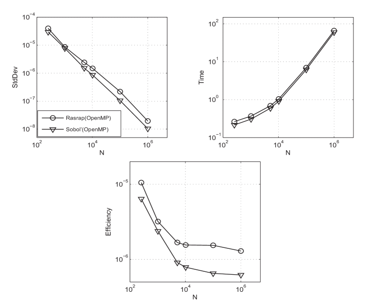
Figure 4: Comparing Rasrap and Sobol’ when pricing caplets with OpenMP on 8 CPU cores

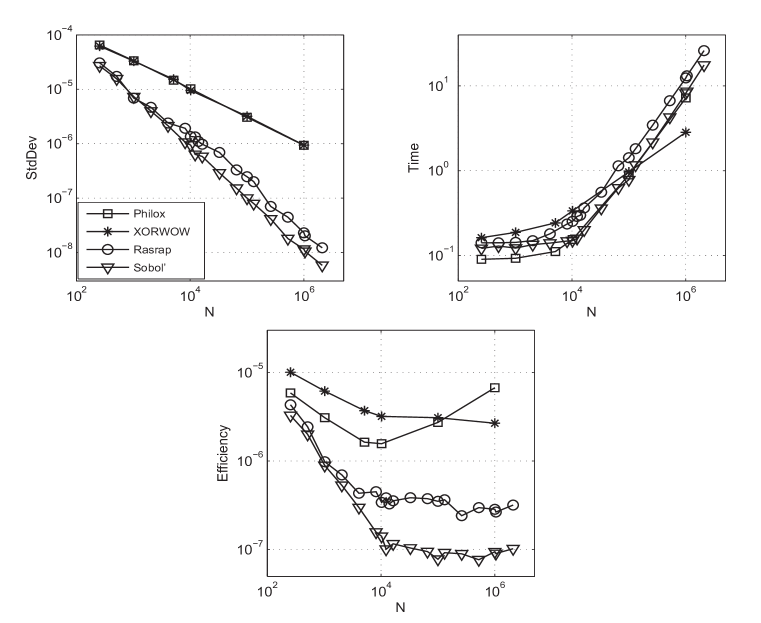
Figure 5: Comparing Philox, XORWOW, Rasrap, and Sobol’, when pricing caplets on GPU

6 Pricing Mortgage-Backed Securities

We follow the mortgage-backed securities (MBS) model given by Caflisch et al. (1997). Consider a security backed by mortgages of length $M$ with fixed interest rate $i_{0}$ which is the interest rate at the beginning of the mortgage. The present value of the security is then

$PV=E(\mathit{v})=E(\sum_{k=1}^{M}u_{k}m_{k})$,

where $E$ is the expectation over the random variables involved in the interest rate fluctuations. The parameters in the model are the following:

$u_{k}=$ discount factor for month $k$

$m_{k}=$ cash flow for month $k$

$i_{k}=$ interest rate for month $k$

$w_{k}=$ fraction of remaining mortgages prepaying in month $k$

$r_{k}=$ fraction of remaining mortgages at month $k$

$c_{k}=$ (remaining annuity at month $k$) $/c$

$c=$ monthly payment

$\xi_{k}=$$N(0,\sigma)$ random variable.

The model defines several of these variables as follows:

$u_{k}=\prod_{j=0}^{k-1}(1+i_{j})^{-1}$

$m_{k}=cr_{k}((1-w_{k})+w_{k}c_{k})$

$r_{k}=\prod_{j=1}^{k-1}(1-w_{j})$

$c_{k}=\sum_{j=0}^{M-k}(1+i_{0})^{-j}$

The interest rate fluctuations and the prepayment rate are given by

$i_{k}=K_{0}e^{\xi_{k}}i_{k-1}=K_{0}^{k}e^{\xi_{1}+\cdots+\xi_{k}}i_{0}$

$w_{k}=K_{1}+K_{2}\arctan(K_{3}i_{k}+K_{4})$

where $K_{1},K_{2},K_{3},K_{4}$ are constants of the model. The constant $K_{0}=e^{-\sigma^{2}/2}$ is chosen to normalize the log-normal distribution so that $E(i_{k})=i_{0}$. The initial interest rate $i_{0}$ also needs to be specified.

We choose the following parameters in our numerical results:

$(i_{0},K_{1},K_{2},K_{3},K_{4},\sigma^{2})=(0.007,0.01,-0.005,10,0.5,0.0004).$

Figure 6 compares OpenMP implementations of Rasrap and Sobol’ sequences on 8 CPU cores. The sample standard deviation of estimates obtained by Rasrap is smaller than that of Sobol’ for every sample size, however, the Sobol’ sequence gives a better rate of convergence. We gain a speedup of 6 with the parallelism using OpenMP compared to the single core version. Rasrap has the better efficiency for all sample sizes.

Figure 7 compares the GPU implementations of Rasrap, Sobol’, Philox, and XORWOW. We observe:

1. The convergence rate for Philox and XORWOW is about $O(N^{-0.5})$;

2. Rasrap gives lower standard deviation than Sobol’, however, the convergence rate for Sobol’ ($O(N^{-0.86})$) is better than Rasrap ($O(N^{-0.68})$);

3. The efficiency of Rasrap is the best among all sequences.

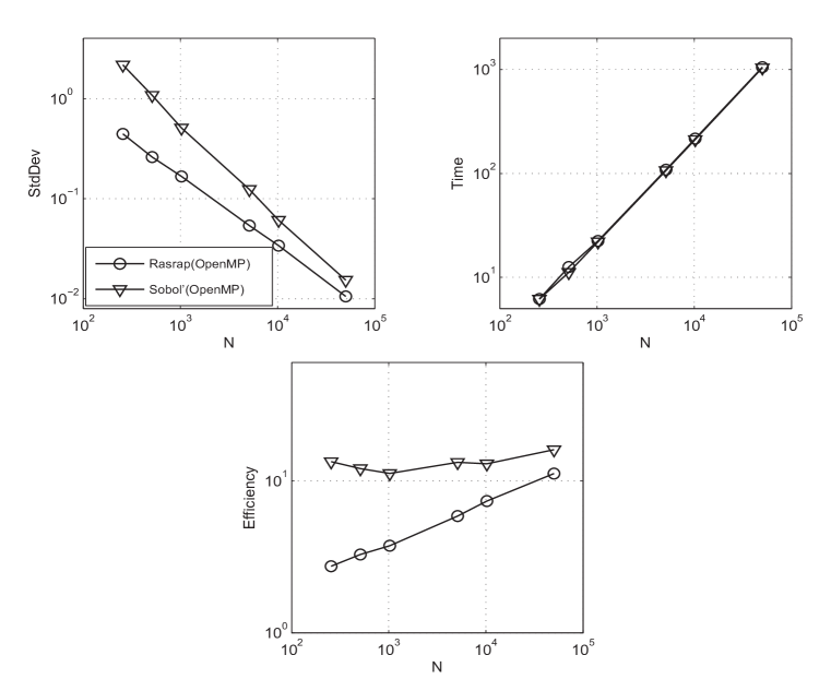
Figure 6: Comparing Rasrap and Sobol’ when pricing MBS with OpenMP on 8 CPU cores

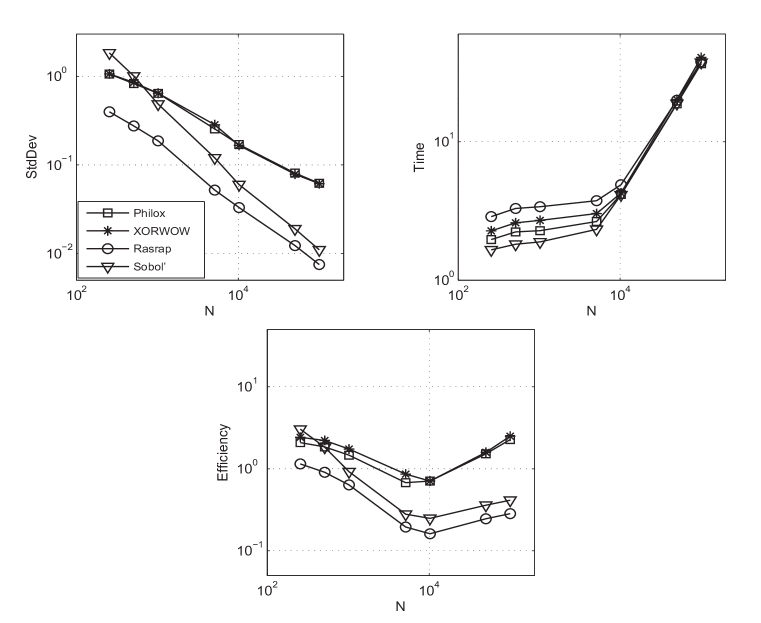
Figure 7: Comparing Philox, XORWOW, Rasrap, and Sobol’, when pricing MBS on GPU

7 Comparing GPU and cluster computing

In Figure 8, we display the GPU speed-up over CPU for both LIBOR and MBS examples. These results only consider the computing time, and the computing time of CPU-Twister is taken as the base value in each example. The largest speed-up is a factor of 95 and it is due to GPU-XORWOW for the LIBOR market model simulation. In the MBS example, GPU-Rasrap speed-up is a factor of 250, and the other GPU sequences give a speed-up of factor 290.

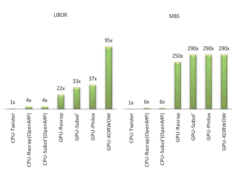
Figure 8: GPU speed-up over CPU in pricing LIBOR caplets and MBS

Finally, to demonstrate the impressive computing power of GPU, we compare GPU with the high performance computing (HPC) cluster at Florida State University. We implement a parallel Sobol’ sequence using MPI, and run simulations for the two examples, LIBOR and MBS. Figure 9 plots the computing time against the number of cores used by the cluster, when the sample size $N$ takes various values. The GPU computing time is plotted as a horizontal line since all the cores of GPU are used in computations. Figure 9 shows that for the LIBOR example, the GPU we used in our computations has equivalent computing power roughly as 128 nodes on the HPC cluster. This is about when the HPC computing time plot reaches the level of GPU computing time, for each $N$. In the MBS example, 256 nodes on the HPC cluster are equivalent to the GPU. We also point out that on a heterogeneous computing environment such as a cluster, continually increasing the number of nodes will not necessarily decrease the running time due to higher cost of communication between nodes and higher probability that slow nodes are used. But for GPUs, a more powerful product with more cores would suggest gains in computing time.

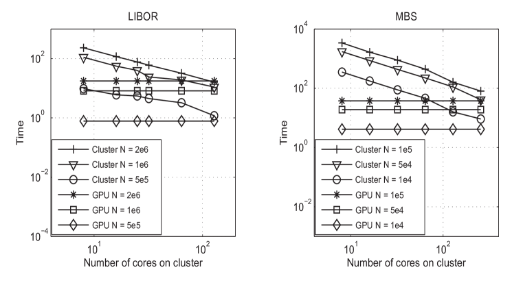
Figure 9: Comparing computing time of GPU and FSU HPC cluster in pricing LIBOR caplets and MBS

References

- Antonov and Saleev (1979) Antonov, I.A. and Saleev, V.M., An economic method of computing - sequences. English translation: U.S.S.R. Comput. Maths. Math. Phys., 1979, 19, 252–256.
- Black (1976) Black, F., The pricing of commodity contracts. Journal of Financial Economics, 1976, 3, 167–179.
- Brace et al. (1997) Brace, A., Gatarek, D. and Musiela, M., The market model of interest rate dynamics. Mathematical Finance, 1997, 7, 127–155.
- Bromley (1996) Bromley, B.C., Quasirandom number generators for parallel Monte Carlo algorithms. Journal of Parallel and Distributed Computing, 1996, 38, 101–104.
- Caflisch et al. (1997) Caflisch, R.E., Morokoff, W., and Owen, A.B., Valuation of mortgage backed securities using brownian bridges to reduce effective dimension. Journal of Computational Finance, 1997, 1, 27–46.
- Chen et al. (2006) Chen, G., Thulasiraman, P. and Thulasiram, R.K., Distributed Quasi-Monte Carlo Algorithm for Option Pricing on HNOWs Using mpC. In Proceedings of the 39th Annual Simulation Symposium, Huntsville, USA, 2–6 April 2006, pp. 90–97, 2006.
- deDoncker et al. (2000) deDoncker, E., Zanny, R., Ciobanu, M. and Guan, Y., Distributed quasi Monte-Carlo methods in a heterogeneous environment. In Proceedings of the 9th Heterogeneous Computing Workshop, Cancun, Mexico, May 2000, pp. 200–206, 2000.
- Glasserman (2003) Glasserman, P., Monte Carlo Methods in Financial Engineering. 2003, Springer.
- Heath et al. (1992) Heath, D., Jarrow, R. and Morton, A., Bond pricing and the term structure of interest rates: a new methodology for contingent claims valuation. Econometrica, 1992, 60, 77–105.
- Hofbauer et al. (2007) Hofbauer, H., Uhl, A. and Zinterhof, P., Parameterization of Zinterhof Sequences for GRID-based QMC Integration. In J. Volkert, T. Fahringer, D. Kranzlmüller, and W. Schreiner, editors, Proceedings of the 2nd Austrian Grid Symposium, volume 221 of books@ocg.at, Innsbruck, Austria, 2007, pp. 91–105, 2007. Austrian Computer Society.
- Jamshidian (1997) Jamshidian, F., Libor and swap market models and measures. Finance and Stochastics, 1997, 1, 43–67.
- Joe and Kuo (2008) Joe, S. and Kuo, F.Y., Constructing Sobol’ sequences with better two-dimensional projections. SIAM J. Sci. Comput., 2008, 30, 2635–2654.
- Li and Mullen (2000) Li, J.X. and Mullen, G.L., Parallel computing of a quasi-Monte Carlo algorithm for valuing derivatives. Parallel Computing, 2000, 26, 641–653.
- Marsaglia (2003) Marsaglia, G., Xorshift RNGs. Journal of Statistical Software, 2003, Vol 8, Issue 14.
- Matsumoto and Nishimura (1998) Matsumoto, M. and Nishimura, T., Dynamic creation of pseudorandom number generators. Monte Carlo and Quasi-Monte Carlo Methods, 1998, Springer 2000, 56–69.
- Matsumoto and Nishimura (1998) Matsumoto, M. and Nishimura, T., Mersenne twister: A 623-dimensionally equidistributed uniform pseudorandom number generator. ACM Transactions on Modeling and Computer Simulations, 1998, 8(1), 3–30.
- Matoušek (1998) Matoušek, J., On the L2-Discrepancy for Anchored Boxes. Journal of Complexity, 1998, 14, 527-556.
- Miltersen et al. (1997) Miltersen, K.R., Sandmann, K. and Sondermann, D., Closed-form solutions for term structure derivatives with lognormal interest rates. Journal of Finance, 1997, 52, 409–430.
- Musiela and Rutkowski (1997) Musiela, M. and Rutkowski, M.,Continuous-time term structure models: forward measure approach. Finance and Stochastics, 1997, 1, 261–292.
- Niederreiter (1992) Niederreiter, H., Random Number Generation and Quasi-Monte Carlo Methods SIAM, Philadelphia, 1992. Vol 8, Issue 14.
- Ökten and Eastman (2004) Ökten, G. and Eastman, W., Randomized quasi-Monte Carlo methods in pricing securities. Journal of Economic Dynamics &Control, 2004, 28, 2399–2426.
- Ökten (2009) Ökten, G., Generalized von Neumann-Kakutani transformation and random-start scrambled Halton sequences. Journal of Complexity, 2009, Vol 25, No 4, 318–331.
- Ökten and Willyard (2010) Ökten, G. and Willyard, M., Parameterization based on randomized quasi-Monte Carlo methods. Parallel Computing, 2010, Vol 36, 415–422.
- Ökten and Srinivasan (2002) Ökten, G. and Srinivasan, A., Parallel Quasi-Monte Carlo Applications on a Heterogeneous Cluster. In K. T. Fang, F. J. Hickernell and H. Niederreiter, editors, Monte Carlo and Quasi-Monte Carlo Methods 2000, Springer-Verlag, Berlin, 2002, pp. 406–421.
- Ökten et al. (2012) Ökten, G., Shah, M. and Goncharov, Y., Random and Deterministic Digit Permutations of the Halton Sequence. In L. Plaskota and H. Woźniakowski, editors, Monte Carlo and Quasi-Monte Carlo Methods 2010, Springer, 2012.
- Saito and Matsumoto (2012) Saito, M. and Matsumoto, M., A deviation of CURAND: standard pseudorandom number generator in CUDA for GPGPU. In 10th International Confrence on Monte carlo and quasi-Monte carlo Methods in Scientific Computing, Sydney, Australia, 13–17 February 2012.
- Salmon et al. (2011) Salmon, J.K., Moraes, M.A., Dror, R.O. and Shaw, D.E., Parallel Random Numbers: As Easy as 1, 2, 3. In SC’11 Proceedings of 2011 International Conference for High Performance Computing, Networking, Storage and Analysis, NY, USA, 2011.
- Schmid and Uhl (1999) Schmid, W. and Uhl, A., Parallel Quasi-Monte Carlo integration using (t,s)-sequences. Lecture Notes in Computer Science, Springer, 2010, 1557, 96–106.
- Schmid and Uhl (2001) Schmid, W. and Uhl, A., Techniques of parallel Quasi-Monte Carlo integration with digital sequences and associated problems. Mathematics and Computers in Simulation, 2001, 55, 249–257.
- Struckmeier (1993) Struckmeier, J., Fast generation of low-discrepancy sequences. Journal of Computational and Applied Mathematics, 1993, 61, 29–41.
- Vandewoestyne and Cools (2006) Vandewoestyne, B. and Cools, R., Good permutations for deterministic scrambled Halton sequences in terms of -discrepancy. Journal of Computational and Applied Mathematics, 2006, 189, 341–361.