On Some Hypergeometric Summations

Abstract

We develop a theoretical study of non-terminating hypergeometric summations with one free parameter. Composing various methods in complex and asymptotic analysis, geometry and arithmetic of certain transcendental curves and rational approximations of irrational numbers, we are able to obtain some necessary conditions of arithmetic flavor for a given hypergeometric sum to admit a gamma product formula. This kind of research seems to be new even in the most classical case of the Gauss hypergeometric series.

1 Introduction

Let ${}_{2}F_{1}(\alpha,\beta;\gamma;z)$ be the Gauss hypergeometric series:

$${}_{2}F_{1}(\alpha,\beta;\gamma;z):=\sum_{k=0}^{\infty}\dfrac{(\alpha)_{k}(\beta)_{k}}{(\gamma)_{k}(1)_{k}}\,z^{k},\qquad(\alpha)_{k}:=\alpha(\alpha+1)\cdots(\alpha+k-1).$$

Given a parameter $\lambda=(p,q,r;a,b;x)\in\mathbb{C}^{5}\times\mathbb{D}$, where $\mathbb{D}=\{x\in\mathbb{C}\,:\,|x|<1\}$ is the open unit disk in the complex plane $\mathbb{C}$, we consider an entire meromorphic function of $w$:

$$f(w)=f(w;\lambda):={}_{2}F_{1}(pw+a,\,qw+b;\,rw;\,x).$$ (1)

We say that $f(w)$ admits a gamma product formula (GPF), if there exist a rational function $S(w)\in\mathbb{C}(w)$; a nonzero complex number $d\in\mathbb{C}^{\times}$; two nonnegative integers $m,n\in\mathbb{Z}_{\geq 0}$; $m$ complex numbers $u_{1},\dots,u_{m}\in\mathbb{C}$; and $n$ complex numbers $v_{1},\dots,v_{n}\in\mathbb{C}$ such that

$$f(w)=S(w)\cdot d^{w}\cdot\dfrac{\varGamma(w+u_{1})\cdots\varGamma(w+u_{m})}{\varGamma(w+v_{1})\cdots\varGamma(w+v_{n})},$$ (2)

where $\varGamma(w)$ is the Euler gamma function. We shall discuss the following.

Problem 1.1

Find a parameter $\lambda=(p,q,r;a,b;x)$ for which $f(w)$ admits a GPF.

A bit of search in the classical literature gives us three solutions in Table 1, where $x=e^{\pm\pi i/3}$ is allowed to lie on the unit circle in the third solution.

$${}_{2}F_{1}\left(-\frac{w}{2}+\frac{3}{4},-\frac{w}{2}+\frac{5}{4};w;-\frac{1}{3}\right) =\left(\frac{8}{9}\right)^{w-3/2}\frac{\varGamma(4/3)\varGamma(w)}{\varGamma(3/2)\varGamma(w-1/6)},$$

$${}_{2}F_{1}\left(3w-\frac{5}{6},3w-\frac{1}{3};3w;\frac{1}{9}\right) =\frac{2^{17/18}}{3^{5/6}}\left(\frac{3^{3}}{2^{4}}\right)^{w}\frac{\varGamma(w+5/36)\varGamma(w+23/36)}{\varGamma(w+2/9)\varGamma(w+5/9)},$$

$${}_{2}F_{1}\left(w,3w-1;2w;e^{\pm\pi i/3}\right) =e^{\mp\pi i/6}\left(2^{2}\cdot 3^{-3/2}\cdot e^{\pm\pi i/2}\right)^{w}\frac{\varGamma(1/2)\varGamma(w+1/2)}{\varGamma(2/3)\varGamma(w+1/3)}.$$

Table 1: Three solutions to Problem 1.1 found in Erdélyi [8].

They are readily derived from formulas (53), (54) and (55)+(56) of Erdélyi [8, Chapter II, §2.8] by affine changes of a variable and the duplication formula for the gamma function. A more extensive search in the literature would give us more solutions. Problem 1.1 naturally extends to the generalized hypergeometric series ${}_{p+1}F_{p}$. Our ultimate goal is to enumerate all solutions to the problem, but it is far beyond the scope of this article even in the most classical case of ${}_{2}F_{1}$, being simply too hard to settle at present. Our aim here is more moderate, that is, to embark on a theoretical study of this very classical problem, but in a direction that has hitherto attracted scant attention.

The subject of hypergeometric evaluations has a long history. Recently it saw an important progress with the development of Wilf-Zeilberger methods [20] and Zeilberger’s algorithms [21, 22], which enabled systematic proofs (and sometimes discoveries) of a lot of combinatorial identities (see also [13, 16]). Gessel [9] and Koepf [12] applied these techniques to terminating hypergeometric sums to give mechanical proofs of classical evaluations in Bailey’s book [3] as well as Gosper, Gessel and Stanton’s “strange” evaluations [10]; see also Apagodu and Zeilberger [2] and Ekhad [7] for more evaluations. In some cases, formulas for terminating series remain true for non-terminating ones, due to Carlson’s theorem in function theory [3, p. 39]. These methods might be useful for our purpose in one direction, that is, toward finding and proving as many solutions as possible, but not in the other direction, that is, toward establishing necessary conditions, as strong as possible, for a given $\lambda=(p,q,r;a,b;x)$ to be a solution. It is expected that $\lambda$ must be subject to some severe constraints, perhaps of arithmetic flavor. In the latter direction we need more transcendental methods based on complex and asymptotic analysis, geometry and arithmetic of certain transcendental curves, as well as on rational approximations of irrational numbers. These are exactly what we want to explore in this article.

Problem 1.1 has a close relative. To state it we say that $f(w)$ is of closed form if

$$\dfrac{f(w+1)}{f(w)}=:R(w)\in\mathbb{C}(w)\,\,:\,\,\mbox{a rational function of $w$}.$$ (3)

Problem 1.2

Find a parameter $\lambda=(p,q,r;a,b;x)$ for which $f(w)$ is of closed form.

Any solution to Problem 1.1 leads to a solution to Problem 1.2. Indeed, by the recurrence formula $\varGamma(w+1)=w\,\varGamma(w)$ for the gamma function, if $f(w)$ admits the product formula (2) then it fulfills condition (3) with rational function

$$R(w)=\dfrac{S(w+1)}{S(w)}\cdot d\cdot\dfrac{(w+u_{1})\cdots(w+u_{m})}{(w+v_{1})\cdots(w+v_{n})}.$$ (4)

Now we can pose a converse question. To formulate it, notice that any rational function $R(w)\in\mathbb{C}(w)$ can be written in the form (4) such that $S(w)\in\mathbb{C}(w)$ is a rational function, $u_{i}-v_{j}$ is not an integer for every $i=1,\dots,m$ and $j=1,\dots,n$, and moreover if $R(w)\in\mathbb{R}(w)$ then $S(w)$, $d$, $P(w):=(w+u_{1})\cdots(w+u_{m})$ and $Q(w):=(w+v_{1})\cdots(w+v_{n})$ should be real (see Lemma 6.1). Such a representation (4) is said to be canonical. Note that in formula (4) one can multiply $S(w)$ by a nonzero (real) constant (if $R(w)$ is real) without changing the form.

Problem 1.3

Does a solution $f(w)$ to Problem 1.2 lead back to a solution to Problem 1.1? Namely, suppose that $f(w)$ satisfies condition (3) with a canonical representation (4) and multiply $S(w)$ by a suitable nonzero constant. Then does $f(w)$ admit GPF (2) ?

We shall give an affirmative solution when $\lambda$ lies in a certain real region (see Theorem 2.3).

There is a method of finding (partial) solutions to Problem 1.2, which we call the method of contiguous relations. It works only when $p,q,r\in\mathbb{Z}$ and relies on the fifteen contiguous relations of Gauss (see e.g. Andrews et. al. [1, §2.5]). Composing a series of contiguous relations yields

$$\begin{split}{}_{2}F_{1}(\alpha+p,\beta+q;\gamma+r;z)&=r(\alpha,\beta;\gamma;z)\,{}_{2}F_{1}(\alpha,\beta;\gamma;z)\\ &\phantom{=}+q(\alpha,\beta;\gamma;z)\,{}_{2}F_{1}(\alpha+1,\beta+1;\gamma+1;z),\end{split}$$ (5)

where $q(\alpha,\beta;\gamma;z)$ and $r(\alpha,\beta;\gamma;z)$ are rational functions of $(\alpha,\beta;\gamma;z)$ depending uniquely upon $(p,q,r)$. Recently Vidunas [18] and Ebisu [4] discussed some computational aspects of formula (5) and showed how to compute $q(\alpha,\beta;\gamma;z)$ and $r(\alpha,\beta;\gamma;z)$ rapidly and efficiently.

Given a parameter $\lambda=(p,q,r;a,b;x)$ with $p,q,r\in\mathbb{Z}$, we put

$$\tilde{f}(w)=\tilde{f}(w;\lambda):={}_{2}F_{1}(pw+a+1,\,qw+b+1;\,rw+1;\,x).$$ (6)

Substituting $(\alpha,\beta;\gamma;z)=(pw+a,qw+b;rw;x)$ into formula (5) we have

$$f(w+1)=R(w)\,f(w)+Q(w)\,\tilde{f}(w),$$ (7)

where $Q(w)=Q(w;\lambda)$ and $R(w)=R(w;\lambda)$ are rational functions of $w$ depending on $\lambda$. If $\lambda$ happens to be such a parameter that $Q(w)$ vanishes identically in $\mathbb{C}(w)$, then three-term relation (7) reduces to the two-term one (3) so that $\lambda$ happens to be a solution to Problem 1.2. The method of contiguous relations is developed by Ebisu [6, 5] (mostly for terminating series) and it will be amplified for non-terminating ones in this article. We say that a solution to Problem 1.2 comes from contiguous relations if it is obtained by this method.

Problem 1.4

When does a solution to Problem 1.2 come from contiguous relations?

In a certain real parameter region we will be able to show that all solutions essentially come from contiguous relations. For the precise statement of this result, including what we mean by essentially, we refer to Theorem 2.7 and a comment right after it.

Problems 1.1 and 1.2 are difficult for a general complex parameter $\lambda=(p,q,r;a,b;x)$. So we content ourselves to suppose that $\lambda$ be real and furthermore to restrict it into a real region

$$p,\,q,\,r\in\mathbb{R},\quad 0<p<r\quad\mbox{or}\quad 0<q<r;\qquad a,\,b\in\mathbb{R};\qquad-1<x<1,$$ (8)

whose $(p,q)$-component forms the cross-shaped domain $D\cup E$ in Figure 1, where $D:=D_{1}\cup D_{2}\cup D_{3}\cup D_{4}$ and $E:=E_{1}\cup E_{2}\cup E_{3}\cup E_{4}$. Of particular interest among (8) is a subregion

$$p,\,q,\,r\in\mathbb{R},\quad 0<p<r\quad\mbox{and}\quad 0<q<r;\qquad a,\,b\in\mathbb{R};\qquad-1<x<1,$$ (9)

whose $(p,q)$-component comprises the central square $D$ in Figure 1.

Figure 1: The real $(p,q)$-plane for a fixed $r>0$.

The main results of this article will be stated either in region (8) or (9) and other parameter regions will be left elsewhere.

The hypergeometric series enjoys well-known $\mathbb{Z}_{2}\ltimes(\mathbb{Z}_{2}\times\mathbb{Z}_{2})$ symmetries:

$${}_{2}F_{1}(\alpha,\,\beta;\,\gamma;\,z) ={}_{2}F_{1}(\beta,\,\alpha;\,\gamma;\,z),$$ (10a)

$$=(1-z)^{\gamma-\alpha-\beta}{}_{2}F_{1}(\gamma-\alpha,\,\gamma-\beta;\,\gamma;\,z),$$ (10b)

$$=(1-z)^{-\alpha}{}_{2}F_{1}(\alpha,\,\gamma-\beta;\,\gamma;\,z/(z-1)),$$ (10c)

$$=(1-z)^{-\beta}{}_{2}F_{1}(\gamma-\alpha,\,\beta;\,\gamma;\,z/(z-1)),$$ (10d)

where transformation (10a) is obvious, (10b) is due to Euler, whereas (10c) and (10d) are due to Pfaff (see [1, Theorem 2.2.5]). They induce symmetries of solutions to Problem 1.1 or 1.2:

$$\lambda=(p,q,r;a,b;x) \mapsto(q,p,r;b,a;x),$$ (11a)

$$\mapsto(r-p,\,r-q,\,r;\,-a,\,-b;\,x),$$ (11b)

$$\mapsto(p,\,r-q,\,r;\,a,\,-b;\,x/(x-1)),$$ (11c)

$$\mapsto(r-p,\,q,\,r;\,-a,\,b;\,x/(x-1)).$$ (11d)

Lemma 1.5

By symmetries (11) the parameter region (8) can be reduced to a subregion

$$p,\,q,\,r\in\mathbb{R},\quad 0<p<r\,\,\,\mbox{and}\,\,\,q\leq p\,\,\,\mbox{and}\,\,\,p+q\leq r;\qquad a,\,b\in\mathbb{R};\qquad 0\leq x<1,$$ (12)

whose $(p,q)$-component forms the “pencil-like” domain $D_{1}\cup E_{1}$ in Figure 1. In a similar manner the parameter region (9) can be reduced to a subregion

$$p,\,q,\,r\in\mathbb{R},\quad 0<q\leq p\,\,\,\mbox{and}\,\,\,p+q\leq r;\qquad a,\,b\in\mathbb{R};\qquad 0\leq x<1,$$ (13)

whose $(p,q)$-component corresponds to the isosceles right triangle $D_{1}$ in Figure 1.

Proof. First we claim that condition (8) can be reduced to

$$p,\,q,\,r\in\mathbb{R},\quad 0<p<r\,\,\,\mbox{and}\,\,\,q<r;\qquad a,\,b\in\mathbb{R};\qquad 0\leq x<1,$$ (14)

whose $(p,q)$-component corresponds to the region $D\cup E_{1}$ in Figure 1. Indeed, we may assume $0<p<r$ in condition (8), for otherwise transformation (11a) takes $0<q<r$ to $0<p<r$. Then $\lambda=(p,q,r;a,b;x)$ is brought to region (14) by transformation (11b) if $q\geq r$ and $0\leq x<1$; by (11c) if $q\geq r$ and $-1<x<0$; and by (11d) if $q<r$ and $-1<x<0$, respectively. Here the map $q\mapsto r-q$ exchanges the conditions $q\geq r$ and $q\leq 0$ $(<r)$, whereas $x\mapsto x/(x-1)$ maps the negative interval $-1<x<0$ to the positive one $0<x<1/2$. Next we show that condition (14) can be reduced to condition (12). If $(p,q)\in E_{1}$ then we are already done. When $(p,q)\in D$, we use transformations (11a) and/or (11b) which keep $x$ invariant. If $(p,q)\in D_{2}\cup D_{3}$, apply (11b) to make $(p,q)\in D_{1}\cup D_{4}$; and if $(p,q)\in D_{4}$, apply (11a) to have $(p,q)\in D_{1}$. These procedures also reduce condition (9) to condition (13). $\Box$

In what follows we shall always exclude the case $x=0$, for which everything is trivial.

2 Main Results

In this section we present the main results together with an outline of this article.

2.1 Elementary Solutions

A solution to Problem 1.1 or 1.2 is said to be elementary if the corresponding function $f(w)$ in definition (1) has at most finitely many poles in the entire complex $w$-plane $\mathbb{C}_{w}$.

Theorem 2.1

In region (8) Problem 1.2 has only two types of elementary solutions. Up to symmetries the first type of elementary solutions are given by

$$q=0,\qquad b\in\mathbb{Z}_{\leq 0},$$ (15)

in which case $f(w)$ itself is a rational function because the series (1) that defines it is terminating. These solutions are attached to the boundary of two strips $E_{1}\cup D\cup E_{3}$ and $E_{2}\cup D\cup E_{4}$ in Figure 1. The second type of elementary solutions are given by

$$p=q=\frac{r}{2}>0,\qquad a=i,\quad b=j-\frac{1}{2},\qquad i,\,j\in\mathbb{Z},$$ (16)

where $a$ and $b$ are permutable by symmetry. They are attached to the “core” of the pencil $D_{1}\cup E_{1}$, namely, to the bullet $\bullet$ in Figure 1. Via the scaling transformation $w\mapsto w/r$, solutions (16) correspond to a contiguous family of degenerate Gauss hypergeometric functions

$$f(w/r)={}_{2}F_{1}\left(\frac{w}{2}+i,\,\frac{w-1}{2}+j,\,w;\,x\right)=S_{ij}(w;x)\cdot\left(\frac{1+\sqrt{1-x}}{2}\right)^{1-w},$$ (17)

where $S_{00}(w;x)=1$ and $S_{ij}(w;x)$ is a rational function of $w$ defined by

$$S_{ij}(w;x)=(1-x)^{-\frac{i+j}{2}}F_{3}\Big{(}i+j,\,j-i;\,1-i-j,\,1+i-j;\,w;\,-\frac{1-\sqrt{1-x}}{2\sqrt{1-x}},\,\frac{1-\sqrt{1-x}}{2}\,\Big{)},$$

with $F_{3}(\alpha_{1},\alpha_{2};\beta_{1},\beta_{2};\gamma;u,v)$ being Appell’s hypergeometric series of two variables:

$$F_{3}(\alpha_{1},\alpha_{2};\beta_{1},\beta_{2};\gamma;u,v):=\sum_{i=0}^{\infty}\sum_{j=0}^{\infty}\frac{(\alpha_{1})_{i}(\alpha_{2})_{j}(\beta_{1})_{i}(\beta_{2})_{j}}{(\gamma)_{i+j}\,i!\,j!}\,u^{i}v^{j}.$$

Indeed, $S_{ij}(w;x)$ is rational in $w$ because the Appell series that defines it is terminating for every $i,j\in\mathbb{Z}$. Functions (17) are instances of Gauss hypergeometric functions with dihedral monodromy groups studied by Vidunas [19]. Theorem 2.1 will be proved in Proposition 4.8.

2.2 Some Examples of Non-Elementary Solutions

$$\begin{array}[]{c|c|c|c|c|c|l}\hline\cr&&&&&&\\[-11.38109pt] r&p&q&x&a&b&f(w+1)/f(w)=R(w)\\[2.84526pt] \cline{1-7}\cr&&&&&&\\[-11.38109pt] 4&1&1&\dfrac{8}{9}&0&\dfrac{1}{4}&\dfrac{4}{3}\cdot\dfrac{(w+2/4)(w+3/4)}{1\cdot 1\cdot(w+2/3)\cdot(w+7/12)}\\[8.53581pt] \cline{5-7}\cr&&&&&&\\[-11.38109pt] &&&&\dfrac{1}{2}&\dfrac{1}{4}&\dfrac{4}{3}\cdot\dfrac{w(w+3/4)}{1\cdot 1\cdot(w+7/12)\cdot(w+1/6)}\\[8.53581pt] \cline{5-7}\cr&&&&&&\\[-11.38109pt] &&&&0&\dfrac{1}{2}&\dfrac{4}{3}\cdot\dfrac{(w+1/4)(w+3/4)}{1\cdot 1\cdot(w+1/3)(w+2/3)\cdot 1}\\[8.53581pt] \cline{1-7}\cr&&&&&&\\[-11.38109pt] 6&1&1&\dfrac{4}{5}&0&\dfrac{1}{2}&\dfrac{3^{6}}{5^{4}}\cdot\dfrac{(w+1/6)(w+2/6)(w+4/6)(w+5/6)}{1\cdot 1\cdot(w+1/5)(w+4/5)\cdot(w+3/10)(w+7/10)}\\[8.53581pt] \cline{5-7}\cr&&&&&&\\[-11.38109pt] &&&&\dfrac{2}{3}&\dfrac{1}{6}&\dfrac{3^{6}}{5^{4}}\cdot\dfrac{w(w+2/6)(w+3/6)(w+5/6)}{1\cdot 1\cdot(w+17/30)(w+23/30)\cdot(w+1/15)(w+4/15)}\\[8.53581pt] \cline{2-7}\cr&&&&&&\\[-11.38109pt] &2&2&\dfrac{3}{4}(3-\sqrt{3})&0&\dfrac{1}{3}&\dfrac{3\sqrt{3}}{2}\cdot\dfrac{(w+2/6)(w+5/6)}{1\cdot 1\cdot(w+3/4)\cdot(w+5/12)}\\[8.53581pt] \cline{2-7}\cr&&&&&&\\[-11.38109pt] &3&1&4(\sqrt{5}-2)&0&\dfrac{1}{6}&\dfrac{27}{125}(5+2\sqrt{5})\cdot\dfrac{(w+3/6)(w+5/6)}{1\cdot 1\cdot 1\cdot(w+17/30)(w+23/30)}\\[8.53581pt] \cline{5-7}\cr&&&&&&\\[-11.38109pt] &&&&0&\dfrac{1}{2}&\dfrac{27}{125}(5+2\sqrt{5})\cdot\dfrac{(w+1/6)(w+5/6)}{1\cdot 1\cdot 1\cdot(w+3/10)(w+7/10)}\\[8.53581pt] \cline{1-7}\cr&&&&&&\\[-11.38109pt] 8&4&2&4(3\sqrt{2}-4)&0&\dfrac{1}{4}&\dfrac{4}{27}(17+12\sqrt{2})\cdot\dfrac{(w+3/8)(w+7/8)}{1\cdot 1\cdot 1\cdot(w+11/24)(w+19/24)}\\[8.53581pt] \hline\cr\end{array}$$

Table 2: Some non-elementary solutions to Problem 1.2 in region (13).

Table 2 exhibits some non-elementary solutions to Problem 1.2 in region (9); they are presented in region (13) upon reduced by symmetries (11). These examples are obtained by the method of contiguous relations. They also lead to solutions to Problem 1.1 due to Theorem 2.3 below. There are also non-elementary solutions to Problem 1.1 not lying in region (9). For example,

$$\begin{split}{}_{2}F_{1}(w,-w+1/2;3w;1/2)&=\dfrac{\csc(\pi/8)}{\sqrt{6}}\cdot\left(\frac{3^{3}}{2^{5}}\right)^{w}\cdot\frac{\varGamma(w+1/3)\varGamma(w+2/3)}{\varGamma(w+3/8)\varGamma(w+5/8)},\\ {}_{2}F_{1}(w+1/3,-w+7/6;3w;1/2)&=\dfrac{2^{5/6}\csc(3\pi/8)}{\sqrt{3}}\cdot\left(\frac{3^{3}}{2^{5}}\right)^{w}\cdot\frac{\varGamma(w)\varGamma(w+2/3)}{\varGamma(w+5/24)\varGamma(w+11/24)}\end{split}$$

are solutions in region (8), whose $(p,q)$-component lies in domain $E_{1}$ of Figure 1.

Problem 2.2

Find necessary conditions on $\lambda=(p,q,r;a,b,;x)$ as well as on the related quantities $d$; $m$, $n$; $u_{1},\dots,u_{m}$ and $v_{1},\dots,v_{n}$, in order for $\lambda$ to be a non-elementary solution to Problem 1.1 or 1.2. Of particular interests to us are arithmetic properties of these quantities.

Of course our ultimate goal is to establish necessary and sufficient conditions in the entire parameter region, but it is far beyond the scope of this article as mentioned in §1. We should content ourselves to establish some necessary conditions upon restricting $\lambda$ to subregion (8) or (9). “Arithmetic properties” in Problem 2.2 refer to such questions as follows. Observe that $p$, $q$ and $r$ in Table 2 are integers; they are trivially so because they come from contiguous relations. But to what extent is this true for a general solution? According to Table 2, the numbers $a$ and $b$ are rational, while $x$ and $d$ are algebraic; moreover, $u_{1},\dots,u_{m}$ and $v_{1},\dots,v_{n}$ are also rational, with $m=n$. Do these observations remain true in general? If so, what kinds of integers occur as the numerators and denominators of those rational numbers?

2.3 Arithmetic Properties

A first thing that can be said about Problem 2.2 in region (8) is the following.

Theorem 2.3

Let $\lambda=(p,q,r;a,b;x)$ be a solution to Problem 1.2 in region (8) and write $R(w)$ in a canonical form (4). Then the gamma product formula (2) is valid with $m=n$. This means that in region (8) any solutions to Problem 1.2 leads back to a solution to Problem 1.1. If the solution is non-elementary then $r$ must be integer with $1\leq m=n\leq r$ and there exist $m$ integers $s_{1},\dots,s_{m}$, mutually distinct modulo $r$, such that

$$u_{i}=s_{i}/r\qquad(i=1,\dots,m).$$ (18)

An essence for the proof of this theorem lies in asymptotic analysis. It consists of investigating the asymptotic behavior of $f(w)$ (see Proposition 3.3) and that of a gamma product expression as in the right-hand side of formula (2) (in §5) and then comparing both results (see Propositions 5.4 and 6.2). Theorem 2.3 will be established at the end of §6 right after Proposition 6.2. It turned out that $r$ must be an integer for any non-elementary solution. How about $p$ and $q$?

$$\begin{array}[]{c|c|c|c|c|c|l}\hline\cr&&&&&&\\[-11.38109pt] r&p&q&x&a&b&f(w+1)/f(w)=R(w)\\[2.84526pt] \cline{1-7}\cr&&&&&&\\[-11.38109pt] 3&\dfrac{1}{2}&\dfrac{1}{2}&\dfrac{4}{5}&0&\dfrac{1}{2}&\dfrac{3^{3}}{5^{2}}\cdot\dfrac{(w+1/3)(w+2/3)}{(w+2/5)(w+3/5)}\\[8.53581pt] \cline{5-7}\cr&&&&&&\\[-11.38109pt] &&&&\dfrac{2}{3}&\dfrac{1}{6}&\dfrac{3^{3}}{5^{2}}\cdot\dfrac{w(w+2/3)}{(w+2/15)(w+8/15)}\\[8.53581pt] \hline\cr\end{array}$$

Table 3: Two non-elementary solutions of type (B).

So far we have an answer to this question only when $\lambda$ is in subregion (9). Put

$$\alpha_{i}:=pu_{i}-a,\qquad\beta_{i}:=qu_{i}-b\qquad(i=1,\dots,m).$$ (19)

Theorem 2.4

For any non-elementary solution $\lambda=(p,q,r;a,b;x)$ in region (9), in addition to $r\in\mathbb{N}:=\mathbb{Z}_{>0}$ mentioned in Theorem 2.3, either $(\mathrm{A})$ or $(\mathrm{B})$ below must be satisfied:

1. $p$, $q\in\mathbb{Z}$;   $p+q+r$ is even;   $\alpha_{i}$, $\beta_{i}\in\mathbb{R}\setminus\mathbb{Z}$   $(i=1,\dots,m)$.

2. $p$, $q\in 1/2+\mathbb{Z}$;   $\alpha_{i}$, $\beta_{i}\in\mathbb{R}\setminus\mathbb{Z}$;   $\alpha_{i}-(-1)^{p+q+r}\,\beta_{i}\in 1/2+\mathbb{Z}$   $(i=1,\dots,m)$.

The dilation constant $d$ in the gamma product formula (2) must be

$$d=\dfrac{r^{r}}{\sqrt{p^{p}\cdot q^{q}\cdot(r-p)^{r-p}\cdot(r-q)^{r-q}\cdot x^{r}\cdot(1-x)^{p+q-r}}}.$$ (20)

Remark 2.5

In Theorem 2.4, if $\lambda=(p,q,r;a,b;x)$ is a solution of type (B) to Problem 1.2, then $\hat{\lambda}:=(2p,2q,2r;a,b;x)$ becomes a solution of type (A) to the problem, with the corresponding rational function $\hat{R}(w)=R(2w)\cdot R(2w+1)$. Indeed, since $f(w;\hat{\lambda})=f(2w;\lambda)$,

$$\dfrac{f(w+1;\hat{\lambda})}{f(w;\hat{\lambda})}=\dfrac{f(2w+2;\lambda)}{f(2w;\lambda)}=\dfrac{f(2w+1;\lambda)}{f(2w;\lambda)}\cdot\dfrac{f(2w+2;\lambda)}{f(2w+1;\lambda)}=R(2w)\cdot R(2w+1)\in\mathbb{C}(w).$$

We call $\hat{\lambda}$ the duplication of $\lambda$. Table 3 exhibits two solutions of type (B), the duplications of which are just those solutions with $(p,q,r)=(1,1,6)$ in Table 2.

The proof of Theorem 2.4 relies on an asymptotic analysis (details of which are developed in §7) and a key lemma below (Lemma 2.6). For a real number $t\in\mathbb{R}$, let $\{t\}:=t-[t]\in[0,\,1)$ denote the fractional part of $t$, where $[t]\in\mathbb{Z}$ stands for the largest integer not exceeding $t$.

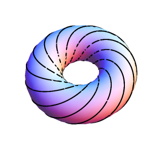
Figure 2: A torus line.

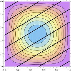
Figure 3: Level curves of $\sin\pi\{x\}\cdot\sin\pi\{y\}$.

Lemma 2.6 (Sine-Sine)

Let $r\in\mathbb{N}$, $p$, $q\in\mathbb{R}^{\times}$ and $\alpha$, $\beta\in\mathbb{R}$. Suppose that

1. there exist positive constants $C>0$ and $h>0$ such that

   $$C\cdot h^{j}\cdot\sin\pi\{pj+\alpha\}\cdot\sin\pi\{qj+\beta\}\to 1\quad\mbox{as}\quad\mathbb{N}\ni j\to\infty,$$ (21)

2. the parities of integers $[pj+\alpha]+[qj+\beta]+rj$ are stationary as $\mathbb{N}\ni j\to\infty$.

Then $h=1$ and either condition $(\mathrm{A})$ or $(\mathrm{B})$ below must be satisfied.

1. $p$, $q\in\mathbb{Z}$;   $p+q+r$ is even;   $\alpha$, $\beta\in\mathbb{R}\setminus\mathbb{Z}$.

2. $p$, $q\in 1/2+\mathbb{Z}$;   $\alpha$, $\beta\in\mathbb{R}\setminus\mathbb{Z}$,   $\alpha-(-1)^{p+q+r}\,\beta\in 1/2+\mathbb{Z}$.

It turns out that condition (21) is equivalent to a seemingly more restrictive condition

$$C\cdot\sin\pi\{pj+\alpha\}\cdot\sin\pi\{qj+\beta\}=1\qquad\mbox{for all}\quad j\in\mathbb{Z}.$$ (22)

The proof of Lemma 2.6 is divided into two parts. In the first part (in §8), Kronecker’s theorem on Diophantine approximations is used to show the rationality of $p$ and $q$; see Figure 3 to get a feel for the discussions around here. In the second part (in §9 and §10), a certain geometry and arithmetic (motivated by condition (22)) for the level curves of the function $\sin\pi\{x\}\cdot\sin\pi\{y\}$ on the torus $(\mathbb{R}/\mathbb{Z})\times(\mathbb{R}/\mathbb{Z})$ (see Figure 3) is used to reduce the possibilities of $(p,q;\alpha,\beta)$ into two types (A) and (B). Theorem 2.4 will be established at the end of §10 (see Proposition 10.2).

2.4 Coming from Contiguous Relations

As mentioned in §1 we can find (partial) solutions to Problem 1.2 by the method of contiguous relations and we may ask how often this class of solutions occur among all solutions to the problem (see Problem 1.4). So far it is only in region (9) that we have an answer to this question. Recall that in this region Problems 1.2 and 1.1 are equivalent by Theorem 2.3.

Theorem 2.7

All non-elementary solutions of type $(\mathrm{A})$ to Problem 1.2 in region (9) come from contiguous relations, where solution types are those mentioned in Theorem 2.4.

If $\lambda$ is a non-elementary solution of type (B), then by Remark 2.5 its duplication $\hat{\lambda}$ is a non-elementary solution of type (A) and hence comes from contiguous relations by Theorem 2.7. In this sense we can say that all non-elementary solutions in region (9) essentially come from contiguous relations. Theorem 2.7 will be proved in Proposition 11.2.

Problem 2.8

Let $\lambda=(p,q,r;a,b;x)$ be a parameter in region (9), where $p$, $q$ and $r$ are a priori supposed to be integers. Find a necessary and sufficient condition in algebraic terms in order for $\lambda$ to be a solution to Problem 1.2 that comes from contiguous relations.

Reduced by symmetries (11) this problem may be discussed in region (13). Given a nonnegative integer $k$, let $\langle\,\varphi(z)\,\rangle_{k}:=\sum_{j=0}^{k}c_{j}z^{j}$ denote the truncation at degree $k$ of a power series $\varphi(z)=\sum_{j=0}^{\infty}c_{j}z^{j}$. In what follows a truncation will always be taken with respect to variable $z$. We introduce a “truncated hypergeometric product” defined by

$$\begin{split}\Phi(w;\lambda)&:=(rw)_{r-1}\,\langle\,{}_{2}F_{1}(\mbox{\boldmath$\alpha$}^{*}(w);z)\cdot{}_{2}F_{1}(\mbox{\boldmath$v$}-\mbox{\boldmath$\alpha$}^{*}(w+1);z)\,\rangle_{r-q-1}\big{|}_{z=x}\\ &\phantom{:}=(rw)_{r-1}\,\langle\,(1-z)^{r-p-q}\cdot{}_{2}F_{1}(\mbox{\boldmath$\alpha$}(w);z)\cdot{}_{2}F_{1}(\mbox{\boldmath$v$}-\mbox{\boldmath$\alpha$}(w+1);z)\,\rangle_{r-q-1}\big{|}_{z=x},\end{split}$$ (23)

where $\mbox{\boldmath$\alpha$}(w):=(pw+a,\,qw+b;\,rw)$, $\mbox{\boldmath$\alpha$}^{*}(w):=((r-p)w-a,\,(r-q)w-b;\,rw)$, $\mbox{\boldmath$v$}:=(1,1;2)$ and the second equality in definition (23) is due to Euler’s transformation (10b). An inspection of definition (23) shows that $\Phi(w;\lambda)$ is a polynomial of $(w;\lambda)=(w;p,q,r;a,b;x)$ over $\mathbb{Q}$ with degree at most $2r-q-2$ in $w$. It is not immediate from definition (23) but can be seen that $\Phi(w;\lambda)$ is more strictly of degree at most $r-1$ in $w$ (see Lemma 11.10). So we can write

$$\Phi(w;\lambda)=\sum_{k=0}^{r-1}\Phi_{k}(\lambda)w^{k}.$$

Theorem 2.9

A parameter $\lambda=(p,q,r;a,b;x)$ in region (13) with $p,q,r\in\mathbb{Z}$ is a solution to Problem 1.2 that comes from contiguous relations if and only if $\Phi(w;\lambda)$ vanishes identically as a polynomial of $w$, that is, if and only if $\lambda$ is a simultaneous root of the following $r$ equations:

$$\Phi_{k}(\lambda)=0\qquad(k=0,1,\dots,r-1).$$ (24)

If a triple $(p,q,r)$ is given then condition (24) yields an overdetermined system of algebraic equations over $\mathbb{Q}$ for an unknown $(a,b;x)$. For a various value of $(p,q,r)$, ask if system (24) admits at least one root and, if so, solve it to obtain an example of solution to Problem 1.4. Actually all solutions in Table 2 were found in this manner with the aid of computer, where the use of Theorem 2.10 below was also helpful. Theorem 2.9 will be proved in Proposition 11.11. It will turn out that (24) leads to an algebraic system involving certain terminating hypergeometric summations, which is in some sense more explicit than (24) itself (see Proposition 11.12).

In view of Theorem 2.7, the method of contiguous relations brings us a further understanding of non-elementary solutions of type (A) in region (13) as in Theorem 2.10 below. To state it, let $p$, $q$ and $r$ be integers such that $0<q\leq p<r$ and $p+q\leq r$, and set

$$\varDelta=\varDelta(z):=(p-q)^{2}z^{2}-2\{(p+q)r-2pq\}z+r^{2}.$$ (25)

Note that $\varDelta(0)=r^{2}>0$ and $\varDelta(1)=(r-p-q)^{2}\geq 0$. If $p\neq q$ then $\varDelta(z)$ is a quadratic polynomial with axis of symmetry $z=1+(p-q)^{-2}\{p(r-p)+q(r-q)\}>1$. If $p=q$ then $\varDelta(z)$ is a linear polynomial with slope $-4p(r-p)<0$. In either case, $\varDelta=\varDelta(z)$ is strictly decreasing and positive in $0\leq z<1$, where we take the branch of $\sqrt{\varDelta}$ so that $\sqrt{\varDelta}>0$. Put

$$Z_{\pm}(z):=\big{\{}r+(p-q)z\pm\sqrt{\varDelta}\big{\}}^{p}\big{\{}r-(p-q)z\pm\sqrt{\varDelta}\big{\}}^{q}\big{\{}(2r-p-q)z-r\mp\sqrt{\varDelta}\big{\}}^{r-p-q}.$$ (26)

Then there exist polynomials $X(z)$ and $Y(z)$ with integer coefficients such that

$$Z_{\pm}(z)=X(z)\pm Y(z)\,\sqrt{\varDelta}.$$ (27)

Observe that $Z_{+}(0)=(-1)^{r-p-q}\,(2r)^{r}$ and $Z_{-}(0)=0$; thus $Y(0)=(-1)^{r-p-q}(2r)^{r-1}\neq 0$ and so the polynomial $Y(z)$ is nonzero. It is not hard to see that the degree of $Y(z)$ is at most $r-1$ if $p\neq q$ and at most $r-p-1$ if $p=q$. The following will be shown in Lemma 11.7:
 $\bullet$ If $r-p-q=0$ then $Y(z)$ has no root in $0\leq z<1$.
 $\bullet$ If $r-p-q$ is a positive even integer then $Y(z)$ has at least one root in $0<z<1$.

To state our result we introduce another truncated hypergeometric product defined by

$$\begin{split}P(w)&:=(rw)_{r}\,\langle\,{}_{2}F_{1}(\mbox{\boldmath$\alpha$}^{*}(w);z)\cdot{}_{2}F_{1}(\mbox{\boldmath$1$}-\mbox{\boldmath$\alpha$}^{*}(w+1);z)\,\rangle_{r-q-1}\big{|}_{z=x}\\ &\phantom{:}=(rw)_{r}\,\langle\,(1-z)^{r-p-q-1}\cdot{}_{2}F_{1}(\mbox{\boldmath$\alpha$}(w);z)\cdot{}_{2}F_{1}(\mbox{\boldmath$e$}_{3}-\mbox{\boldmath$\alpha$}(w+1);z)\,\rangle_{r-q-1}\big{|}_{z=x},\end{split}$$ (28)

where $\mbox{\boldmath$\alpha$}(w)$ and $\mbox{\boldmath$\alpha$}^{*}(w)$ are the same as in definition (23), $\mbox{\boldmath$1$}:=(1,1;1)$, $\mbox{\boldmath$e$}_{3}:=(0,0;1)$ and the second equality in (28) follows from Euler’s transformation (10b). An inspection of definition (28) shows that $P(w)$ is a polynomial of degree at most $2r-q-1$ in $w$. It turns out that if $r-p-q\geq 1$ then $P(w)$ is more strictly of degree at most $r$ in $w$ (see Lemma 11.10).

Regarding the number $x$ and the rational function $R(w)$ in formula (3) we have the following.

Theorem 2.10

For any non-elementary solution $\lambda=(p,q,r;a,b;x)$ of type $(\mathrm{A})$ to Problem 1.2 in region (13), the following statements must be true:

1. The number $x$ is a root of $Y(z)$ in the interval $0<z<1$. In particular $x$ is an algebraic number of degree at most $r-1$ if $p\neq q$ and at most $r-p-1$ if $p=q$, respectively.

2. The integer $r-p-q$ is positive and even.

3. $P(w)$ is exactly of degree $r$ and the rational function $R(w)$ in formula (3) is given by

   $$R(w)=(1-x)^{r-p-q-1}\cdot\dfrac{(rw)_{r}}{P(w)}.$$ (29)

   Moreover, in $\mathbb{C}[w]$ the polynomial $P(w)$ admits a division relation

   $$P(w)\,\big{|}\,(pw+a+1)_{p-1}(qw+b+1)_{q-1}((r-p)w-a)_{r-p}((r-q)w-b)_{r-q}.$$ (30)

Assertions (1) and (2) of Theorem 2.10 will be proved in Proposition 11.8, while assertion (3) will be established in Proposition 11.11, respectively.

Remark 2.11

A few comments on Theorem 2.10 should be in order at this stage.

1. In assertion (1) the condition that $x$ should be a root of $Y(z)$ is equivalent to the equation $\Phi_{r-1}(\lambda)=0$ in system (24) (see Lemma 11.10). The degree bound for $x$ there is by no means optimal. In fact, for every solution $\lambda$ known to the author, $Y(z)$ is reducible and $x$ is either rational or quadratic. Since $Y(z)$ depends only on $(p,q;r)$, so does the root $x$ and hence the dilation constant $d$ in formula (20), that is, $d$ is independent of $(a,b)$.

2. Exactly $r$ among all the $2r-2$ factors on the right side of division relation (30) appear as factors of $P(w)$. It is yet to be decided which $r$ should be chosen. This question seems quite hard in general, but it has something to do with certain terminating hypergeometric sums (see Proposition 11.14). At least one can say that $P(w)$ contains each of

   $$\textstyle w+\frac{r-p-1-a}{r-p};\quad w+\frac{r-q-1-b}{r-q};\quad w+\frac{a+p-1}{p}\quad\mbox{(if $p\geq 2$)};\quad w+\frac{b+q-1}{q}\quad\mbox{(if $q\geq 2$)},$$ (31)

   as a factor (see the end of §11.5). In any case, division relation (30) provides us with much, though not full, information about the numbers $u_{1},\dots,u_{n}$ in formula (2). In particular they are real numbers (rational numbers if so are $a$ and $b$).

3. It often occurs in formula (29) that the numerator $(rw)_{r}$ and denominator $P(w)$ have some factors in common that can be canceled to get a reduced representation. Or rather the author knows no example in region (9) for which such a cancellation does not occur.

3 Stationary Phase Method for Euler’s Integral

In this section $f(w)$ is just the function defined by formula (1), that is, it may or may not be a solution to Problem 1.1 or 1.2. We consider it in the parameter region (8), which can be reduced to subregion (12) by Lemma 1.5. Rather we may and shall work in the intermediate region (14). Thus under condition (14) we study the asymptotic behavior of $f(w)$ as $w\to\infty$ on a right half-plane. Euler’s integral representation for the hypergeometric function allows us to write $f(w)=\psi(w)f_{1}(w)$, where $\psi(w)$ and $f_{1}(w)$ are given by

$$\psi(w) =\frac{\varGamma(rw)}{\varGamma(pw+a)\varGamma((r-p)w-a)},$$ (32)

$$f_{1}(w) =\int_{0}^{1}t^{pw+a-1}(1-t)^{(r-p)w-a-1}(1-xt)^{-qw-b}dt.$$ (33)

The improper integral in formula (33) converges if $p\,\mathrm{Re}(w)+a>0$ and $(r-p)\,\mathrm{Re}(w)-a>0$. Due to assumption (14) this condition is satisfied on the right half-plane $\mathrm{Re}(w)\geq R_{1}$, if

$$R_{1}>\max\{-a/p,\,a/(r-p)\}\,(\geq 0).$$ (34)

The gamma factor $\psi(w)$ can be estimated by Stirling’s formula, which states that $\varGamma(t)\sim\sqrt{2\pi}\,e^{-t}\,t^{t-1/2}$ as $t\to\infty$ uniformly on every proper subsector of the sector $|\arg(t)|<\pi$, where $*\sim**$ indicates that the ratio of $*$ and $**$ tends to $1$ as $t\to\infty$ in the region considered. It is convenient to note a slightly generalized version of Stirling’s formula: for any $\alpha>0$ and $\beta\in\mathbb{C}$,

$$\varGamma(\alpha t+\beta)\sim\sqrt{2\pi}\,\alpha^{\beta-1/2}\,(\alpha/e)^{\alpha t}\,t^{\alpha t+\beta-1/2}\qquad\mbox{as}\quad t\to\infty,$$ (35)

which is valid on the same sector as above and is easily derived from the original formula.

Lemma 3.1

The function $\psi(w)$ is holomorphic and admits a uniform estimate

$$\psi(w)\sim A_{1}\cdot B_{1}^{w}\cdot w^{1/2},$$

on the right half-plane $\mathrm{Re}(w)>0$, where $A_{1}$ and $B_{1}$ are given by

$$A_{1}=\frac{1}{\sqrt{2\pi}}\cdot\frac{(r-p)^{a+1/2}}{p^{a-1/2}\,r^{1/2}},\qquad B_{1}=\frac{r^{r}}{p^{p}\,(r-p)^{r-p}}.$$

Proof. The poles of $\psi(w)$ are contained in the arithmetic progression $\{-j/r\}_{j=0}^{\infty}$ and so $\psi(w)$ is holomorphic on $\mathrm{Re}(w)>0$. By Stirling’s formula (35) we have

$$\psi(w) \sim\frac{\sqrt{2\pi}\,r^{-1/2}\,(r/e)^{rw}\,w^{rw-1/2}}{\sqrt{2\pi}\,p^{a-1/2}\,(p/e)^{pw}\,w^{pw+a-1/2}\cdot\sqrt{2\pi}\,(r-p)^{-a-1/2}\,((r-p)/e)^{(r-p)w}\,w^{(r-p)w-a-1/2}}$$

$$=\frac{1}{\sqrt{2\pi}}\cdot\frac{(r-p)^{a+1/2}}{p^{a-1/2}\,r^{1/2}}\cdot\left(\frac{r^{r}}{p^{p}\,(r-p)^{r-p}}\right)^{w}\cdot w^{1/2}=A_{1}\cdot B_{1}^{w}\cdot w^{1/2},$$

as $w\to\infty$ uniformly on $\mathrm{Re}(w)>0$. This proves the lemma. $\Box$

The integral in formula (33) can be written

$$f_{1}(w)=\int_{0}^{1}\Phi(t)^{w}\,\eta(t)\,dt=\int_{0}^{1}e^{-w\phi(t)}\,\eta(t)\,dt,$$ (36)

where $\Phi(t)$, $\phi(t)$ and $\eta(t)$ are defined by

$$\begin{split}\Phi(t)&=t^{p}(1-t)^{r-p}(1-xt)^{-q},\qquad\phi(t)=-\log\Phi(t),\\ \eta(t)&=t^{a-1}(1-t)^{-a-1}(1-xt)^{-b}.\end{split}$$ (37)

We apply the stationary phase method to evaluate integral (36). Observe that

$$\phi^{\prime}(t)=\frac{\phi_{1}(t)}{t(1-t)(1-xt)},\qquad\phi_{1}(t):=-(r-q)xt^{2}+\{(p-q)x+r\}t-p,$$

where $\phi_{1}(t)$ is a concave quadratic function thanks to assumption (14). Here recall that the trivial case $x=0$ is excluded. Since $\phi_{1}(0)=-p<0$ and $\phi_{1}(1)=(r-p)(1-x)>0$, there is a unique root $0<t_{0}<1$ of the quadratic equation $\phi_{1}(t)=0$. Note that $\phi_{1}^{\prime}(t_{0})>0$ and hence

$$\phi^{\prime\prime}(t_{0})=\frac{\phi_{1}^{\prime}(t_{0})}{t_{0}(1-t_{0})(1-xt_{0})}=\frac{-2(r-q)xt_{0}+(p-q)x+r}{t_{0}(1-t_{0})(1-xt_{0})}>0,$$

because $t_{0}$ lies strictly to the left of the axis of symmetry for the parabola $\phi_{1}(t)$.

Lemma 3.2

The function $f_{1}(w)$ is holomorphic and admits a uniform estimate

$$f_{1}(w)\sim\sqrt{2\pi}\,\frac{\eta(t_{0})}{\sqrt{\phi^{\prime\prime}(t_{0})}}\,\Phi(t_{0})^{w}\,w^{-1/2}\qquad\mbox{as}\quad w\to\infty,$$ (38)

on the right half-plane $\mathrm{Re}(w)\geq R_{1}$, where $R_{1}$ is any number satisfying condition (34).

Proof. The function $f_{1}(w)$ is holomorphic on $\mathrm{Re}(w)\geq R_{1}$ by the convergence condition for the improper integral (33) mentioned above. Asymptotic formula (38) is obtained by the standard stationary phase method, so only an outline of its derivation will be included below. Suppose that $\arg w=0$ for simplicity. Then the path of integration is just the real interval $0<t<1$ as taken in formula (36), where the phase function $\phi(t)$ attains its minimum at $t=t_{0}$ so that the vicinity of this point has the greatest contribution to the value of integral (36). Observing that

$$\phi(t)=\phi(t_{0})+\frac{1}{2}\phi^{\prime\prime}(t_{0})(t-t_{0})^{2}+O((t-t_{0})^{3}),\quad\eta(t)=\eta(t_{0})+O(t-t_{0}),\quad\mbox{as}\quad t\to t_{0},$$

we have for any sufficiently small positive number $\varepsilon>0$,

$$f_{1}(w) \sim\int_{t_{0}-\varepsilon}^{t_{0}+\varepsilon}e^{-w\{\phi(t_{0})+\frac{1}{2}\phi^{\prime\prime}(t_{0})(t-t_{0})^{2}\}}\,\eta(t)\,dt\sim\Phi(t_{0})^{w}\int_{t_{0}-\varepsilon}^{t_{0}+\varepsilon}e^{-\frac{1}{2}w\phi^{\prime\prime}(t_{0})(t-t_{0})^{2}}\,\eta(t_{0})\,dt$$

$$\sim\eta(t_{0})\,\Phi(t_{0})^{w}\int_{-\infty}^{\infty}e^{-\frac{1}{2}w\phi^{\prime\prime}(t_{0})t^{2}}\,dt=\dfrac{\eta(t_{0})}{\sqrt{\frac{1}{2}w\phi^{\prime\prime}(t_{0})}}\,\Phi(t_{0})^{w}\int_{-\infty}^{\infty}e^{-t^{2}}dt,$$

from which formula (38) follows, where we made a change of variable $t\sqrt{\frac{1}{2}w\phi^{\prime\prime}(t_{0})}\mapsto t$ to obtain the last equality.

Figure 4: A path of steepest descent in the $t$-plane.

This argument carries over for a general complex variable $w$ on the right half-plane $\mathrm{Re}(w)\geq R_{1}$ if the path of integration is deformed as in Figure 4. $\Box$

Lemmas 3.1 and 3.2 are put together to yield the following.

Proposition 3.3

The function $f(w)$ is holomorphic and admits a uniform estimate

$$f(w)\sim A\cdot B^{w}\qquad\mbox{as}\quad w\to\infty,$$ (39)

on the right half-plane $\mathrm{Re}(w)\geq R_{1}$, where $A$ and $B$ are given by

$$A=\frac{(r-p)^{a+1/2}}{p^{a-1/2}\,r^{1/2}}\cdot\frac{\eta(t_{0})}{\sqrt{\phi^{\prime\prime}(t_{0})}},\qquad B=\frac{r^{r}}{p^{p}\,(r-p)^{r-p}}\cdot\Phi(t_{0}).$$ (40)

Proof. This proposition follows immediately from Lemmas 3.1 and 3.2. $\Box$

4 Poles and Their Residues

Also in this section $f(w)$ is just the function defined by formula (1), which may or may not be a solution to Problem 1.1 or 1.2, while condition (14) is retained. We discuss the pole structure of the function $f(w)$. Any pole of $f(w)$ is simple and must lie in the arithmetic progression

$$W:=\{w_{j}:=-j/r\}_{j=0}^{\infty},$$ (41)

but $f(w)$ may be holomorphic at some points of (41). In order to know whether a given point $w_{j}$ is actually a pole or not, we need to calculate the residue of $f(w)$ at $w=w_{j}$.

Lemma 4.1

The residue of $f(w)$ at $w=w_{j}$ admits a hypergeometric expression

$$\underset{\scriptstyle w=w_{j}}{\mathrm{Res}}\,f(w)=C_{j}\cdot{}_{2}F_{1}(a_{j},\,b_{j};\,j+2;\,x)\qquad(j=0,1,2,\dots),$$ (42)

where $a_{j}:=pw_{j}+j+a+1$, $b_{j}:=qw_{j}+j+b+1$ and

$$C_{j}:=\frac{(-1)^{j}}{r}\cdot\frac{(pw_{j}+a)_{j+1}\,(qw_{j}+b)_{j+1}}{j!\,(j+1)!}\,x^{j+1}.$$ (43)

Proof. Let $j$ and $k$ be nonnegative integers. At the point $w=w_{j}$ the $k$-th summand of the hypergeometric series $f(w)={}_{2}F_{1}(pw+a,qw+b;rw;x)$ has residue

$$\underset{\scriptstyle w=w_{j}}{\mathrm{Res}}\,\frac{(pw+a)_{k}(qw+b)_{k}}{(rw)_{k}\,k!}x^{k}=\begin{cases}0&(k\leq j),\\[5.69054pt] \dfrac{1}{r}\cdot\dfrac{(-1)^{j}}{j!}\cdot\dfrac{(pw_{j}+a)_{k}(qw_{j}+b)_{k}}{(k-j-1)!\,k!}\,x^{k}&(k\geq j+1).\end{cases}$$

Sum of these numbers over $k\geq j+1$ gives the residue of $f(w)$ at $w=w_{j}$. Putting $k=i+j+1$,

$$\underset{\scriptstyle w=w_{j}}{\mathrm{Res}}\,f(w) =\dfrac{x^{j+1}}{r}\cdot\dfrac{(-1)^{j}}{j!}\sum_{i=0}^{\infty}\dfrac{(pw_{j}+a)_{i+j+1}\,(qw_{j}+b)_{i+j+1}}{(i+j+1)!\,i!}\,x^{i}$$

$$=\frac{x^{j+1}}{r}\cdot\frac{(-1)^{j}}{j!}\sum_{i=0}^{\infty}\frac{(pw_{j}+a)_{j+1}(pw_{j}+a+j+1)_{i}\cdot(qw_{j}+b)_{j+1}(qw_{j}+b+j+1)_{i}}{(j+1)!\,(j+2)_{i}\,i!}\,x^{i}$$

$$=C_{j}\sum_{i=0}^{\infty}\frac{(a_{j})_{i}\,(b_{j})_{i}}{(j+2)_{i}\,i!}\,x^{i}=C_{j}\cdot{}_{2}F_{1}(a_{j},\,b_{j};\,j+2;\,x),$$

where $(t)_{i+j+1}=(t)_{j+1}\,(t+j+1)_{i}$ is used in the second equality. This proves formula (42). $\Box$

For every sufficiently large integer $j$, Lemma 4.1 reduces it to an elementary arithmetic to know whether $f(w)$ is holomorphic or has a pole at $w=w_{j}$.

Lemma 4.2

There exists a positive integer $j_{0}$ such that for any integer $j\geq j_{0}$ the function $f(w)$ is holomorphic at $w=w_{j}$ if and only if either condition (44a) or (44b) below holds:

$$r(a+i) =pj\qquad\mbox{for some}\quad i\in\{0,\dots,j\},$$ (44a)

$$r(b+i) =qj\qquad\mbox{for some}\quad i\in\{0,\dots,j\}.$$ (44b)

Proof. Observe that $a_{j}=\{(r-p)j+r(a+1)\}/r$ and $b_{j}=\{(r-q)j+r(b+1)\}/r$, where $r-p$ and $r-q$ are positive numbers due to assumption (14). Take an integer $j_{0}$ so that

$$j_{0}>\max\left\{-\frac{r(a+1)}{r-p},\,-\frac{r(b+1)}{r-q},\,0\right\}.$$

Then $a_{j}$ and $b_{j}$ are positive for every $j\geq j_{0}$ so that $(a_{j})_{i}$ and $(b_{j})_{i}$ are also positive for every $i\geq 1$. Since $0\leq x<1$ by assumption (14), we have ${}_{2}F_{1}(a_{j},b_{j};j+2;x)\geq{}_{2}F_{1}(a_{j},b_{j};j+2;0)=1$. Thus formula (42) tells us that $\underset{\scriptstyle w=w_{j}}{\mathrm{Res}}\,f(w)=0$, that is, $f(w)$ is holomorphic at $w=w_{j}$ if and only if $C_{j}=0$. In view of definition (43) this condition is equivalent to

$$(pw_{j}+a)_{j+1}\,(qw_{j}+b)_{j+1}=0,$$

which in turn holds true exactly when either condition (44a) or (44b) is satisfied. $\Box$

Lemma 4.2 poses the problem of finding nonnegative integers $j$ with property (44a), which will be referred to as problem (44a); this convention also applies to property (44b). We wish to know whether each problem has infinitely many solutions and, if so, how the solutions look like. These questions will be answered after the following preliminary lemma.

Lemma 4.3

Let $\lambda$ and $\mu$ be coprime integers with $1\leq\mu<\lambda$ and $\nu$ a real number. Let $J$ be the set of all nonnegative integers $j$ such that $\nu+\lambda i=\mu j$ for some $i\in\{0,\dots,j\}$. Then $J$ is nonempty if and only if $\nu$ is an integer. If this is the case then $J$ comprises an arithmetic progression $J=\{j_{*}+\lambda k\}_{k=0}^{\infty}$ with $j_{*}\equiv\nu\mu_{*}\mod\lambda$, where $\mu_{*}\in\mathbb{Z}$ is inverse to $\mu\mod\lambda$.

Proof. If $J$ is nonempty and has an element $j\in J$ with the corresponding number $i\in\{0,\dots,j\}$, then evidently $\nu=\mu j-\lambda i$ must be an integer. Conversely suppose that $\nu$ is an integer. Since $\lambda$ and $\mu$ are coprime, there exist integers $i^{\prime}$ and $j^{\prime}$ such that $\nu=\mu j^{\prime}-\lambda i^{\prime}$, that is, $\nu+\lambda i^{\prime}=\mu j^{\prime}$. Consider $i=i^{\prime}+\mu k$ and $j=j^{\prime}+\lambda k$ for $k\in\mathbb{Z}$. Note that $j-i=j^{\prime}-i^{\prime}+(\lambda-\mu)k$. Since $\mu$ and $\lambda-\mu$ are positive, one has $0\leq i\leq j$ and $\nu+\lambda i=\mu j$ for every sufficiently large $k$. Thus $j\in J$ and so $J$ is nonempty. Supposing that $J$ is nonempty, let $j_{*}$ be the smallest element of $J$ with the corresponding $i_{*}$. It is easy to see the inclusion $\{j_{*}+\lambda k\}_{k=0}^{\infty}\subset J$. Conversely, if $j$ is any element of $J$ with the corresponding $i$, then taking the difference from the smallest element yields $\lambda(i-i_{*})=\mu(j-j_{*})$. Since $\lambda$ and $\mu$ are coprime, there is a nonnegative integer $k$ such that $i-i_{*}=\mu k$ and $j-j_{*}=\lambda k$ so that $j=j_{*}+\lambda k$ belongs to the arithmetic progression $\{j_{*}+\lambda k\}_{k=0}^{\infty}$. It follows from $\nu+\lambda i_{*}=\mu j_{*}$ that $j_{*}\equiv(\mu j_{*})\mu_{*}\equiv(\nu+\lambda i_{*})\mu_{*}\equiv\nu\mu_{*}\mod\lambda$. $\Box$

Lemma 4.4

Problem (44a) has infinitely many solutions if and only if

$$p/r=p_{1}/r_{p}\in\mathbb{Q},\quad p_{1},\,r_{p}\in\mathbb{Z},\quad(p_{1},r_{p})=1,\quad 1\leq p_{1}<r_{p};\quad a_{1}:=r_{p}\,a\in\mathbb{Z},$$ (45)

for some $p_{1}$ and $r_{p}$, in which case all solutions to (44a) comprise an arithmetic progression

$$J_{p}=\{j_{p}+r_{p}k\}_{k=0}^{\infty},\qquad\mbox{with}\quad j_{p}\equiv a_{2}:=a_{1}p_{2}\mod r_{p},$$ (46)

where $p_{2}$ is an $(\mbox{any})$ integer such that $p_{1}p_{2}\equiv 1\mod r_{p}$. On the other hand, problem (44b) has infinitely many solutions if and only if either condition (15) is satisfied, in which case all solutions to (44b) comprise an arithmetic progression $J_{q}=\{-b+k\}_{k=0}^{\infty};$ or otherwise,

$$q/r=q_{1}/r_{q}\in\mathbb{Q},\quad q_{1},\,r_{q}\in\mathbb{Z},\quad(q_{1},r_{q})=1,\quad 1\leq q_{1}<r_{q};\quad b_{1}:=r_{q}\,b\in\mathbb{Z},$$ (47)

for some $q_{1}$ and $r_{q}$, in which case all solutions to (44b) comprise an arithmetic progression

$$J_{q}=\{j_{q}+r_{q}k\}_{k=0}^{\infty},\qquad\mbox{with}\quad j_{q}\equiv b_{2}:=b_{1}q_{2}\mod r_{q},$$ (48)

where $q_{2}$ is an $(\mbox{any})$ integer such that $q_{1}q_{2}\equiv 1\mod r_{q}$.

Proof. If problem (44a) has infinitely many solutions, then of course it has two solutions $j<j^{\prime}$ with $i$ and $i^{\prime}$ being the corresponding values of $i$. Then $r(a+i)=pj$ and $r(a+i^{\prime})=pj^{\prime}$, whose difference makes $r(i^{\prime}-i)=p(j^{\prime}-j)$. Thus $p/r=(i^{\prime}-i)/(j^{\prime}-j)$ must be a rational number. From $0<p<r$ in assumption (14) one has $1\leq p_{1}<r_{p}$ in the reduced representation $p_{1}/r_{p}$ of the rational number $p/r$. In terms of $p_{1}$ and $r_{p}$, the condition (44a) is equivalent to

$$a_{1}+r_{p}i=p_{1}j\qquad\mbox{for some}\quad i\in\{0,\dots,j\}.$$ (49)

Now that $p_{1}$ and $r_{p}$ are coprime integers such that $1\leq p_{1}<r_{p}$, Lemma 4.3 can be applied to problem (49) to establish the assertion for problem (44a).

We proceed to the assertion for problem (44b). First we consider the case $q=0$. In this case condition (44b) becomes $b+i=0$ with $0\leq i\leq j$, that is, $b=-i$ is a nonpositive integer and $j\geq i=-b$. Thus problem (44b) has infinitely many solutions precisely when condition (15) is satisfied, in which case the integers $j\geq-b$ give all solutions. Next we consider the case where $q$ is nonzero. The proof is just the same as for problem (44a) except that we have to show $0<q<r$ if problem (44b) has infinitely many solutions. Note that $q<r$ is evident from condition (14). To show $0<q$, suppose the contrary that $q<0$ and problem (44b) has infinitely many solutions $j\in J$ with the corresponding $i\in I$’s. Since $q$ and $r$ are nonzero and $r(b+i)=qj$, the correspondence $J\to I$, $j\mapsto i$ is a one-to-one mapping. The infinite set $J$ contains an infinite subset $J^{\prime}$ such that $j>0$ for every $j\in J^{\prime}$. The corresponding subset $I^{\prime}\subset I$ is also infinite. For every $i\in I^{\prime}$ we have $r(b+i)=qj<0$ and so $0\leq i<-b$. But this is absurd and hence we must have $0<q<r$. $\Box$

To describe how (46) and (48) intersect we require another preliminary lemma.

Lemma 4.5

Consider two arithmetic progressions $J_{1}=\{j_{1}+\lambda_{1}k\}_{k=0}^{\infty}$ and $J_{2}=\{j_{2}+\lambda_{2}k\}_{k=0}^{\infty}$, where $\lambda_{1}$ and $\lambda_{2}$ are positive integers while $j_{1}$ and $j_{2}$ are integers. Then $J_{1}$ and $J_{2}$ intersect if and only if $j_{1}\equiv j_{2}\mod\lambda_{3}:=\gcd\{\lambda_{1},\,\lambda_{2}\}$. In this case the intersection $J_{1}\cap J_{2}$ comprises an arithmetic progression $J_{3}=\{j_{3}+(\lambda_{1}\lambda_{2}/\lambda_{3})k\}_{k=0}^{\infty}$, where $j_{3}\equiv j_{1}\equiv j_{2}\mod\lambda_{3}$.

Proof. If $J_{1}$ and $J_{2}$ have an element in common, say, $j_{1}+\lambda_{1}k_{1}=j_{2}+\lambda_{2}k_{2}$, then clearly $j_{1}-j_{2}=\lambda_{2}k_{2}-\lambda_{1}k_{1}\equiv 0\mod\lambda_{3}$. Conversely suppose that $j_{1}\equiv j_{2}\mod\lambda_{3}$. Then there exist integers $k_{1}^{\prime}$ and $k_{2}^{\prime}$ such that $j_{1}-j_{2}=\lambda_{2}k_{2}^{\prime}-\lambda_{1}k_{1}^{\prime}$, that is, $j_{1}+\lambda_{1}k_{1}^{\prime}=j_{2}+\lambda_{2}k_{2}^{\prime}$. Consider the number $j:=j_{1}+\lambda_{1}k_{1}=j_{2}+\lambda_{2}k_{2}$, where $k_{1}:=k_{1}^{\prime}+(\lambda_{2}/\lambda_{3})l$ and $k_{2}:=k_{2}^{\prime}+(\lambda_{1}/\lambda_{3})l$ with $l\in\mathbb{Z}$. For every sufficiently large $l$, one has $k_{1}\geq 0$ and $k_{2}\geq 0$ so that $j\in J_{1}\cap J_{2}$ and hence $J_{1}\cap J_{2}$ is nonempty. Suppose now that $J_{1}\cap J_{2}$ is nonempty and let $j_{3}=j_{1}+\lambda_{1}k_{1}^{\prime}=j_{2}+\lambda_{2}k_{2}^{\prime}$ be its smallest element. Then it is easy to see the inclusion $\{j_{3}+(\lambda_{1}\lambda_{2}/\lambda_{3})k\}_{k=0}^{\infty}\subset J_{1}\cap J_{2}$. Conversely, if $j=j_{1}+\lambda_{1}k_{1}=j_{2}+\lambda_{2}k_{2}$ is any element of $J_{1}\cap J_{2}$, then its difference from the smallest element yields $\lambda_{1}(k_{1}-k_{1}^{\prime})=\lambda_{2}(k_{2}-k_{2}^{\prime})\geq 0$, or equivalently $(\lambda_{1}/\lambda_{3})(k_{1}-k_{1}^{\prime})=(\lambda_{2}/\lambda_{3})(k_{2}-k_{2}^{\prime})\geq 0$. Since $\lambda_{1}/\lambda_{3}$ and $\lambda_{2}/\lambda_{3}$ are coprime, there exists a nonnegative integer $k$ such that $k_{1}-k_{1}^{\prime}=(\lambda_{2}/\lambda_{3})k$ and $k_{2}-k_{2}^{\prime}=(\lambda_{1}/\lambda_{3})k$. Thus $j=j_{1}+\lambda_{1}\{k_{1}^{\prime}+(\lambda_{2}/\lambda_{3})k\}=j_{3}+(\lambda_{1}\lambda_{2}/\lambda_{3})k$. This gives the reverse inclusion $J_{1}\cap J_{2}\subset\{j_{3}+(\lambda_{1}\lambda_{2}/\lambda_{3})k\}_{k=0}^{\infty}$. Finally $j_{3}\equiv j_{1}\equiv j_{2}\mod\lambda_{3}$ is immediate from $j_{3}=j_{1}+\lambda_{1}k_{1}^{\prime}=j_{2}+\lambda_{2}k_{2}^{\prime}$. The proof is complete. $\Box$

Lemma 4.6

If conditions (45) and (47) are satisfied, then $J_{p}$ and $J_{q}$ intersect if and only if

$$a_{2}\equiv b_{2}\mod r_{pq}:=\gcd\{r_{p},\,r_{q}\},$$ (50)

in which case the intersection $J_{p}\cap J_{q}$ comprises an arithmetic progression

$$J_{pq}:=\{\,j_{pq}+(r_{p}r_{q}/r_{pq})\,k\,\}_{k=0}^{\infty}\qquad\mbox{with}\quad j_{pq}\equiv a_{2}\equiv b_{2}\mod r_{pq}.$$ (51)

Proof. This lemma is an immediate consequence of Lemmas 4.4 and 4.5. $\Box$

For a subset $A\subset\mathbb{R}$ bounded below or above its density is defined by the limit

$$\delta(A):=\lim_{t\to\infty}\frac{1}{t}\,\#\{x\in A\,:\,\pm x\leq t\},$$

where $\#$ denotes the cardinality of a set and plus (resp. minus) sign is chosen when $A$ is bounded below (resp. above). We consider only those subsets for which density is well defined. When density is considered for two or more subsets, they are simultaneously bounded below or above. Two sets $A$ and $B$ are said to be commensurable if they share all but a finite number of elements, in which case we write $A\circeq B$. As basic properties of density we have

$$\delta(A\cup B) =\delta(A)+\delta(B)-\delta(A\cap B),$$

$$\delta(A^{\prime}) =|\mu|^{-1}\ \delta(A)\qquad\mbox{for}\quad A^{\prime}:=\mu A+\nu\quad\mbox{with}\quad(\mu,\nu)\in\mathbb{R}^{\times}\times\mathbb{R},$$

$$\delta(A) =\delta(B)\qquad\mbox{if}\quad A\circeq B.$$

Let $W_{\mathrm{hol}}\subset W$ be the set of all points in (41) at which $f(w)$ is holomorphic and $J$ the set of all nonnegative integers $j$ that satisfy condition (44a) or (44b). Lemma 4.2 implies that

$$W_{\mathrm{hol}}\circeq-J/r,\qquad\delta(W_{\mathrm{hol}})=r\,\delta(J).$$ (52)

Lemma 4.7

If condition (15) is satisfied then $\delta(J)=1$. Otherwise, $\delta(J)$ is given as in Table 4, depending upon whether condition (45), (47) or (50) is true $(\mathrm{T})$ or false $(\mathrm{F})$.

case	(45)	(47)	(50)	$\delta(J)$
I	F	F	—	$0$
II	F	T	—	$1/r_{q}$
III	T	F	—	$1/r_{p}$
IV	T	T	F	$1/r_{p}+1/r_{q}$
V	T	T	T	$1/r_{p}+1/r_{q}-r_{pq}/(r_{p}r_{q})$

Table 4: Density $\delta(J)$ in the failure of condition (15).

Proof. Note that the whole arithmetic progression (41) has density $r$. If condition (15) holds true then our hypergeometric sum is terminating so that $f(w)$ is a rational function, clearly having only a finite number of poles. If $f(w)$ has only a finite number of poles then all but a finite number of points in the set (41) belong to $W_{\mathrm{hol}}$ so that $\delta(W_{\mathrm{hol}})=r$ and hence $\delta(J)=1$ by formula (52). Now suppose that condition (15) is not satisfied. In case I of Table 4, it is obvious that $J$ is empty and $\delta(J)=0$. In case II one has $J=J_{q}$ and $\delta(J)=\delta(J_{q})=1/r_{q}$. Similarly in case III one has $J=J_{p}$ and $\delta(J)=\delta(J_{p})=1/r_{p}$. In cases IV and V one has $J=J_{p}\cup J_{q}$ and $\delta(J)=\delta(J_{p}\cup J_{q})=\delta(J_{p})+\delta(J_{q})-\delta(J_{p}\cap J_{q})$, so formulas (46), (48) and (51) yield $\delta(J)=1/r_{p}+1/r_{q}$ in case IV and $\delta(J)=1/r_{p}+1/r_{q}-r_{pq}/(r_{p}r_{q})$ in case V. $\Box$

Proposition 4.8

The function $f(w)$ has only a finite number of poles if and only if either condition (15) or (16) is satisfied. If this is the case then $f(w)$ yields an elementary solution to Problem 1.1 and hence to Problem 1.2. Therefore Theorem 2.1 follows.

Proof. If condition (15) holds then our hypergeometric sum is terminating so that $f(w)$ is a rational function, evidently having only a finite number of poles and giving an elementary solution to Problem 1.1. Suppose that condition (15) is not satisfied and so we are in one of the five cases in Table 4. As is seen in the proof of Lemma 4.7, $f(w)$ has only a finite number of poles only when $\delta(J)=1$. So let us consider when $\delta(J)=1$ occurs. Obviously it cannot occur in cases I, II and III, because $r_{p}\geq 2$ and $r_{q}\geq 2$. A simple check shows that in case IV it is again impossible unless $r_{p}=r_{q}=2$. This also implies that it is not possible in case V either, since the presence of positive term $r_{pq}/(r_{p}r_{q})>0$ forces $\delta(J)<1$ even when $r_{p}=r_{q}=2$. Finally, in case IV with $r_{p}=r_{q}=2$ the validity of conditions (45) and (47) shows that $p_{1}=q_{1}=1$, $p=q=r/2$ and $2a$, $2b\in\mathbb{Z}$, while the failure of condition (50) means that $2a$ and $2b$ must have distinct parities. By symmetry (11a) we may assume that $2a$ is even and $2b$ is odd, that is, $a=i$ and $b=j-1/2$ for some $i$, $j\in\mathbb{Z}$. This leads to condition (16). Conversely, if condition (16) is satisfied then formula (17) follows from an analysis of Vidunas [19]. This formula evidently shows that $f(w)$ yields an elementary solution to Problem 1.1. $\Box$

5 Gamma Product Formula

We continue to work on the parameter region (14). Suppose that $f(w)$ is a solution to Problem 1.2 with $R(w)$ in condition (3) being of the form (4), where representation (4) may or may not be in a canonical form, for example, it may be just the reduced expression of $R(w)$ with $S(w)\equiv 1$, while $S(w)$, $d$, $P(w):=(w+u_{1})\cdots(w+u_{m})$ and $Q(w):=(w+v_{1})\cdots(w+v_{n})$ are supposed to be real, since $R(w)$ is real. Consider the entire meromorphic function defined by

$$g(w):=S(w)\cdot d^{w}\cdot\frac{\varGamma(w+u_{1})\cdots\varGamma(w+u_{m})}{\varGamma(w+v_{1})\cdots\varGamma(w+v_{n})}.$$ (53)

Put $u:=u_{1}+\cdots+u_{m}$ and $v:=v_{1}+\cdots+v_{n}$; they are real because $P(w)$ and $Q(w)$ are real.

Lemma 5.1

There exists a constant $R_{2}$ such that on the right half-plane $\mathrm{Re}(w)\geq R_{2}$ the function $g(w)$ is holomorphic, nowhere vanishing, and admits a uniform estimate

$$g(w)\sim S_{0}\cdot(2\pi)^{(m-n)/2}\left(de^{n-m}\right)^{w}\cdot w^{-(m-n)/2+u-v+s_{0}}\cdot e^{(m-n)w\log w},$$

where $S_{0}\in\mathbb{R}^{\times}$ and $s_{0}\in\mathbb{Z}$ are determined by the condition $S(w)\sim S_{0}w^{s_{0}}$ as $w\to\infty$.

Proof. Take a number $R_{2}\in\mathbb{R}$ in such a manner that all the points $-u_{1},\dots,-u_{m};-v_{1},\dots,-v_{n}$ as well as all the zeros and poles of $S(w)$ are strictly to the left of the vertical line $\mathrm{Re}(w)=R_{2}$. Then it is clear from the locations of its poles and zeros that $g(w)$ is holomorphic and non-vanishing on the half-plane $\mathrm{Re}(w)\geq R_{2}$. By Stirling’s formula (35), we have

$$g(w) =S(w)\cdot d^{w}\frac{\prod_{i=1}^{m}\varGamma(w+u_{i})}{\prod_{j=1}^{n}\varGamma(w+v_{j})}\sim S_{0}w^{s_{0}}\cdot d^{w}\frac{\prod_{i=1}^{m}\sqrt{2\pi}\,e^{-w}\,w^{w+u_{i}-1/2}}{\prod_{j=1}^{n}\sqrt{2\pi}\,e^{-w}\,w^{w+v_{j}-1/2}}$$

$$=S_{0}w^{s_{0}}\cdot d^{w}\cdot(2\pi)^{(m-n)/2}\,e^{(n-m)w}\,w^{(m-n)(w-1/2)+u-v}$$

$$=S_{0}\cdot(2\pi)^{(m-n)/2}\cdot(de^{n-m})^{w}\cdot w^{-(m-n)/2+u-v+s_{0}}\cdot w^{(m-n)w}$$

$$=S_{0}\cdot(2\pi)^{(m-n)/2}\cdot(de^{n-m})^{w}\cdot w^{-(m-n)/2+u-v+s_{0}}\cdot e^{(m-n)w\log w}.$$

uniformly on $\mathrm{Re}(w)\geq R_{2}$. This establishes the lemma. $\Box$

Observe that $g(w)$ satisfies the same recurrence relation (3) as the function $f(w)$. So it is natural to compare $f(w)$ with $g(w)$ or in other words to think of the ratio

$$h(w):=\frac{f(w)}{g(w)}.$$ (54)

It is clear that $h(w)$ is an entire meromorphic function that does not vanish identically.

Lemma 5.2

$h(w)$ is an entire holomorphic function which is periodic of period one. For any $R_{3}>\max\{R_{1},\,R_{2},\,1\}$ there exists a constant $A_{2}>0$ such that

$$|h(w)|\leq A_{2}\cdot K^{\mathrm{Re}(w)}\cdot|w|^{(n-m)\{\mathrm{Re}(w)-1/2\}+v-u-s_{0}}\cdot e^{-(n-m)\arg(w)\cdot\mathrm{Im}(w)},$$ (55)

on $\mathrm{Re}(w)\geq R_{3}$, where $K:=e^{m-n}B/d$ with $B$ being the positive constant in Proposition 3.3.

Proof. Since $f(w)$ and $g(w)$ satisfy the same recurrence relation (3), their ratio $h(w)$ must be a periodic function of period one. From Proposition 3.3 and Lemma 5.1 the function $h(w)$ has no poles on $\mathrm{Re}(w)\geq R_{3}$ and so holomorphic there. The periodicity then implies that $h(w)$ must be holomorphic on the entire complex plane. In view of $\left|e^{w\log w}\right|=e^{\mathrm{Re}(w\log w)}=e^{\mathrm{Re}(w)\cdot\log|w|-\mathrm{Im}(w)\cdot\arg(w)}=|w|^{\mathrm{Re}(w)}e^{-\mathrm{Im}(w)\cdot\arg(w)}$, Lemma 5.1 implies that

$$|g(w)|\sim|S_{0}|\cdot(2\pi)^{(m-n)/2}\left(de^{n-m}\right)^{\mathrm{Re}(w)}\cdot|w|^{(m-n)\{\mathrm{Re}(w)-1/2\}+u-v+s_{0}}\cdot e^{-(m-n)\mathrm{Im}(w)\cdot\arg(w)},$$

uniformly on $\mathrm{Re}(w)\geq R_{3}$. Since $g(w)$ has no zero there, there is a constant $A_{3}>0$ such that

$$|g(w)|\geq A_{3}\cdot\left(de^{n-m}\right)^{\mathrm{Re}(w)}\cdot|w|^{(m-n)\{\mathrm{Re}(w)-1/2\}+u-v+s_{0}}\cdot e^{-(m-n)\mathrm{Im}(w)\cdot\arg(w)},$$

on $\mathrm{Re}(w)\geq R_{3}$. On the other hand, by Proposition 3.3 there exists a constant $A_{4}>0$ such that $|f(w)|\leq A_{4}\cdot B^{\mathrm{Re}(w)}$ on $\mathrm{Re}(w)\geq R_{3}$. Thus estimate (55) holds true with $A_{2}:=A_{4}/A_{3}$. $\Box$

Lemma 5.3

We have $m=n$ in formulas (4) and (53). Moreover $h(w)$ is a nonzero constant.

Proof. First we show $m\leq n$. Suppose the contrary $m>n$. Estimate (55) with real $w$ reads $|h(w)|\leq A_{2}\cdot K^{w}\cdot w^{-(m-n)(w-1/2)+v-u-s_{0}}$ for every $w\geq R_{3}$. Fix any $w\in\mathbb{R}$ and take a positive integer $k_{0}$ such that $w+k_{0}\geq R_{3}$. Since $h(w)$ is periodic of period one, for any integer $k\geq k_{0}$,

$$|h(w)|=|h(w+k)| \leq A_{2}\cdot K^{w+k}\cdot(w+k)^{-(m-n)(w+k-1/2)+v-u-s_{0}}$$

$$=A_{2}\cdot K^{w}\cdot(1+w/k)^{\rho}\cdot(1+w/k)^{-(m-n)k}\cdot k^{\rho}\cdot(K/k^{m-n})^{k}$$

$$\sim A_{2}\cdot K^{w}\cdot e^{-(m-n)w}\cdot k^{\rho}\cdot(K/k^{m-n})^{k}\quad\mbox{as}\quad k\to+\infty,$$

where $\rho:=-(m-n)(w-1/2)+v-u-s_{0}$. Since we are assuming that $m-n>0$ there exists an integer $k_{1}\geq k_{0}$ such that$0<K/k_{1}^{m-n}\leq 1/2$. Then there exists a constant $A_{5}>A_{2}\cdot K^{w}\cdot e^{-(m-n)w}$ such that $|h(w)|\leq A_{5}\cdot k^{\rho}\cdot 2^{-k}$ for every $k\geq k_{1}$. Letting $k\to+\infty$ we have $h(w)=0$ for every $w\in\mathbb{R}$. By the unicity theorem for holomorphic functions, $h(w)$ must vanish identically. But this is absurd because $h(w)$ is nontrivial and thus we have proved $m\leq n$.

Next we show that $h(w)$ is a nonzero constant. We make use of estimate (55) on the strip $R_{3}\leq\mathrm{Re}(w)\leq R_{3}+1$, where we recall $R_{3}>1$. On this strip $K^{\mathrm{Re}(w)}$ are bounded while $|w|^{(n-m)\{\mathrm{Re}(w)-1/2\}+v-u-s_{0}}\leq|w|^{\mu}\leq A_{6}(1+|\mathrm{Im}(w)|^{\mu})$ for some constant $A_{6}$, where $\mu$ is a nonnegative number with $\mu\geq(n-m)(R_{2}-1/2)+v-u-s_{0}$. On the strip, if $|\mathrm{Im}(w)|\geq R_{3}+1$ then $|\arg(w)|\geq\pi/4$ and $\arg(w)\cdot\mathrm{Im}(w)\geq(\pi/4)|\mathrm{Im}(w)|$. So there is a constant $A_{7}$ such that

$$|h(w)|\leq A_{7}(1+|\mathrm{Im}(w)|^{\mu})e^{-\pi(n-m)|\mathrm{Im}(w)|/4},$$ (56)

holds for any point $w$ on the strip $R_{3}\leq\mathrm{Re}(w)\leq R_{3}+1$ such that $|\mathrm{Im}(w)|\geq R_{3}+1$. Estimate (56) remains true on the entire strip if $A_{7}$ is chosen sufficiently large. Moreover this estimate extends to the entire complex plane, since both sides of it are periodic functions of period one. In particular, in view of $m\leq n$, estimate (56) yields $|h(w)|\leq A_{7}\cdot(1+|\mathrm{Im}(w)|^{\mu})\leq A_{7}\cdot(1+|w|^{\mu})$ for every $w\in\mathbb{C}$. Liouville’s theorem then implies that $h(w)$ must be a polynomial. But the fundamental theorem of algebra tells us that a polynomial can be a periodic function only when it is a constant. Hence $h(w)$ must be a constant, which is nonzero as $h(w)$ is nontrivial. Finally we show that $m=n$. We already know that $m\leq n$. If $m<n$ then the right-hand side of estimate (56) would tend to zero as $|\mathrm{Im}(w)|\to\infty$. But this contradicts the fact that $h(w)$ is a nonzero constant. Thus we must have $m=n$. The proof is complete. $\Box$

Recall that we can multiply the rational function $S(w)$ by any nonzero constant without changing the form of expression (4). Thus after multiplying $S(w)$ by a suitable constant if necessary, we may conclude that $h(w)\equiv 1$ in Lemma 5.3 and so definitions (53) and (54) yield

$$f(w)\equiv g(w):=S(w)\cdot d^{w}\cdot\frac{\varGamma(w+u_{1})\cdots\varGamma(w+u_{m})}{\varGamma(w+v_{1})\cdots\varGamma(w+v_{m})}.$$ (57)

Proposition 5.4

If $f(w)$ is a solution to Problem 1.2 in region (14), then we have an identity (57) with $m=n$, $S_{0}=A$, $d=B$ and $v=u+s_{0}$ in formula (4), where $S_{0}\in\mathbb{R}^{\times}$ and $s_{0}\in\mathbb{Z}$ are the numbers defined by the asymptotic condition $S(w)\sim S_{0}w^{s_{0}}$ as $w\to\infty$; $A$ and $B$ are the constants defined in Proposition 3.3; and $u:=u_{1}+\cdots+u_{m}$ and $v:=v_{1}+\cdots+v_{n}$.

Proof. We have only to evaluate $S_{0}$, $d$ and $v$. Now that we have $m=n$ by Lemma 5.3, the asymptotic formula in Lemma 5.1 reads $g(w)\sim S_{0}\cdot d^{w}\cdot w^{u-v+s_{0}}$ as $w\to\infty$ on the half-plane $\mathrm{Re}(w)\geq R_{2}$. Compare this with the asymptotic formula $f(w)\sim A\cdot B^{w}$ in Proposition 3.3. The identity $f(w)\equiv g(w)$ then implies that $S_{0}=A$, $d=B$ and $u-v+s_{0}=0$. $\Box$

6 Rational Functions in Canonical Form

We make a general discussion about rational functions in order to put representation (4) in a canonical form. Given a rational function $R(w)\in\mathbb{C}(w)$, consider an expression of the form

$$R(w)=\frac{S(w+1)}{S(w)}\cdot d\cdot\frac{P(w)}{Q(w)},$$ (58)

where $S(w)$ is a rational function, $d$ is a nonzero constant, and $P(w)$ and $Q(w)$ are monic polynomials. $P(w)$ and $Q(w)$ are said to be strongly coprime if $P(w)$ and $Q(w+j)$ are coprime over $\mathbb{C}$ for every integer $j$, in which case representation (58) is said to be canonical. We remark that Gosper [11] considered expression (58) in a similar but somewhat different situation where $P(w)$ and $Q(w+j)$ were coprime for every nonnegative integer $j$ with $S(w)$ being a polynomial.

Lemma 6.1

Any rational function $R(w)\in\mathbb{C}(w)$ admits a canonical representation (58). If $R(w)\in\mathbb{R}(w)$ then $d$, $P(w)$, $Q(w)$ and $S(w)$ can be taken to be real.

Proof. Start with the reduced expression $R(w)=d\cdot P_{0}(w)/Q_{0}(w)$, where $P_{0}(w)$ and $Q_{0}(w)$ are coprime monic polynomials. If they are strongly coprime then we are done with $P(w)=P_{0}(w)$, $Q(w)=Q_{0}(w)$ and $S(w)=1$. Otherwise the argument proceeds as follows. Suppose that there is a representation (58) in which $P(w)$ and $Q(w)$ are coprime but not strongly coprime. Then either there exists a positive integer $i$ such that $P(w+i)$ and $Q(w)$ have a common factor or there exists a positive integer $j$ such that $P(w)$ and $Q(w+j)$ have a common factor. In the former case there is a number $\alpha\in\mathbb{C}$ such that $(w+\alpha)|P(w)$ and $(w+\alpha+i)|Q(w)$. Put

$$P_{1}(w):=\frac{P(w)}{w+\alpha},\qquad Q_{1}(w):=\frac{Q(w)}{w+\alpha+i},\qquad S_{1}(w):=\frac{S(w)}{(w+\alpha)_{i}}.$$ (59)

In the latter case there is a number $\beta\in\mathbb{C}$ such that $(w+\beta+j)|P(w)$ and $(w+\beta)|Q(w)$. Put

$$P_{1}(w):=\frac{P(w)}{w+\beta+j},\qquad Q_{1}(w):=\frac{Q(w)}{w+\beta},\qquad S_{1}(w):=S(w)\cdot(w+\beta)_{j}.$$ (60)

In either case it is easy to see that $P_{1}(w)$ and $Q_{1}(w)$ are coprime monic polynomials such that

$$\frac{S_{1}(w+1)}{S_{1}(w)}\cdot d\cdot\frac{P_{1}(w)}{Q_{1}(w)}=\frac{S(w+1)}{S(w)}\cdot d\cdot\frac{P(w)}{Q(w)}=R(w),$$

with $\deg P_{1}(w)=\deg P(w)-1$ and $\deg Q_{1}(w)=\deg Q(w)-1$. If $P_{1}(w)$ and $Q_{1}(w)$ are strongly coprime then we are done. Otherwise, repeat the same procedure. This process must terminate in finite steps because the degrees of $P(w)$ and $Q(w)$ decrease by one in each step.

The proof of the second assertion requires a slight modification of the above argument. Suppose that $R(z)$ is real. Then $d$, $P_{0}(w)$ and $Q_{0}(w)$ above can be taken to be real. The induction procedure $(P,Q,S)\mapsto(P_{1},Q_{1},S_{1})$ in formula (59) resp. (60) carries over if $\alpha$ resp. $\beta$ is real. But if $\alpha$ resp. $\beta$ is not real then formula (59) resp. (60) should be replaced by

$$P_{1}(w) :=\textstyle\frac{P(w)}{(w+\alpha)(w+\bar{\alpha})}, Q_{1}(w) :=\textstyle\frac{Q(w)}{(w+\alpha+i)(w+\bar{\alpha}+i)}, S_{1}(w) :=\textstyle\frac{S(w)}{(w+\alpha)_{i}\cdot(w+\bar{\alpha})_{i}},$$

$$P_{1}(w) :=\textstyle\frac{P(w)}{(w+\beta+j)(w+\bar{\beta}+j)}, Q_{1}(w) :=\textstyle\frac{Q(w)}{(w+\beta)(w+\bar{\beta})}, S_{1}(w) :=S(w)\cdot(w+\beta)_{j}\cdot(w+\bar{\beta})_{j},$$

respectively. This is well defined since if a real polynomial has a non-real root then its complex conjugate is also a root of the same polynomial. The modified procedure keeps realness, so that the real initial data $(d,P_{0},Q_{0})$ leads to a final real output $(S,d,P,Q)$. $\Box$

Proposition 6.2

Let $f(w)$ be a non-elementary solution to Problem 1.2 in region (14). If representation (4) is canonical, then we have $m=n\geq 1$, the number $r$ must be a positive integer with $r\geq m$ and there exist integers $s_{1},\dots,s_{m}$ mutually distinct modulo $r$ such that (18) holds.

Proof. Let $W_{\mathrm{pole}}$ denote the set of all poles of $f(w)$, which is an infinite set since $f(w)$ is assumed to be non-elementary. In formula (57) the poles of $\varGamma(w+u_{1})\cdots\varGamma(w+u_{m})$ and those of $\varGamma(w+v_{1})\cdots\varGamma(w+v_{m})$ constitute two families of arithmetic progressions

$$U_{i} :=\{-u_{i}-k\}_{k=0}^{\infty}\qquad\,\,(i=1,\dots,m),$$ (61)

$$V_{j} :=\{\,-v_{j}-k\,\}_{k=0}^{\infty}\qquad(j=1,\dots,m),$$ (62)

respectively. Since representation (4) is canonical, $U_{i}$ and $V_{j}$ are disjoint for every $i,j=1,\dots,m$, so that $W_{\mathrm{pole}}$ is commensurable to the union $\bigcup_{i=1}^{m}U_{i}$, where this union is disjoint because all poles of $f(w)$ are simple so that $u_{i}-u_{j}$ is not an integer for every $i\neq j$, that is,

$$W_{\mathrm{pole}}\stackrel{{\scriptstyle\circ}}{{=}}\coprod_{i=1}^{m}U_{i}.$$ (63)

Thus when expression (4) is canonical, $f(w)$ is non-elementary if and only if $m\geq 1$.

Take $i=1$ and $k$ sufficiently large in the arithmetic progression (61). Equation (57) then shows that $w=-u_{1}-k$ and $w=-u_{1}-k-1$ are poles of $f(w)=g(w)$, so that they must lie in the arithmetic progression (41). Thus there exist nonnegative integers $j_{1}$ and $j_{2}$ with $j_{1}<j_{2}$ such that $-u_{1}-k=-j_{1}/r$ and $-u_{1}-k-1=-j_{2}/r$. Taking their difference gives $1=(j_{2}-j_{1})/r$, which shows that $r=j_{2}-j_{1}$ must be a positive integer. Similarly, for each $i=1,\dots,m$ there exists an integer $k_{i}$ such that $w=-u_{i}-k_{i}$ is a pole of $g(w)=f(w)$ and so it must lie in the arithmetic progression (41), namely, it can be written $-u_{i}-k_{i}=-j_{i}/r$ for some integer $j_{i}$. If we put $s_{i}:=j_{i}+rk_{i}$ then formula (18) holds true. Note that $s_{1},\dots,s_{m}$ are mutually distinct modulo $r$, because $U_{i},\dots,U_{m}$ are mutually disjoint. $\Box$

Note that putting Propositions 5.4 and 6.2 together yields Theorem 2.3.

7 Asymptotics of the Residues

Throughout this section let $\lambda=(p,q,r;a,b,x)$ and the associated $f(w)=f(w;\lambda)$ be a non-elementary solution to Problem 1.2 in region (14) with formula (4) in a canonical form. The poles of $f(w)$ are commensurable to the disjoint union of $m$ arithmetic progressions $U_{i}$ $(i=1,\dots,m)$ as in formula (63). In view of formulas (41) and (18) the general term of $U_{i}$ is expressed as $-u_{i}-k=-(rk+s_{i})/r=w_{j}$ with $j=rk+s_{i}$. In this situation, if we put

$$\mathrm{Res}_{k}^{(i)}:=\underset{\scriptstyle w=w_{j}}{\mathrm{Res}}\,f(w),\quad C_{k}^{(i)}:=C_{j},\quad F_{k}^{(i)}:={}_{2}F_{1}(a_{j},\,b_{j};\,j+2;\,x),$$

using the notation of Lemma 4.1, then formula (42) reads

$$\mathrm{Res}_{k}^{(i)}=C_{k}^{(i)}\cdot F_{k}^{(i)}.$$ (64)

We study the asymptotic behavior of $\mathrm{Res}_{k}^{(i)}$ as $k\to\infty$ for a fixed $i=1,\dots,m$.

Lemma 7.1

Let $B$ and $t_{0}$ be the same constants as in definition (40) and put

$$\xi(t) :=t^{-2p/r-1}(1-t)^{2p/r-3}(1-xt)^{2q/r-1},$$ (65)

$$\widetilde{A} :=\dfrac{p^{a+2p/r-1/2}}{(r-p)^{a+2p/r-3/2}\cdot r^{1/2}}\cdot\dfrac{\xi(t_{0})}{\eta(t_{0})\sqrt{\phi^{\prime\prime}(t_{0})}},$$ (66)

where $\phi(t)$ and $\eta(t)$ are defined by formula (37). Then for each $i=1,\dots,m$, we have

$$F_{k}^{(i)}\sim\{(1-x)^{(p+q-r)u_{i}-a-b}\widetilde{A}B^{u_{i}+2/r}\}\cdot\{(1-x)^{p+q-r}B\}^{k}\qquad\mbox{as}\quad k\to\infty.$$ (67)

Proof. Euler’s transformation (10b) and the definitions of $a_{j}$ and $b_{j}$ in Lemma 4.1 yield

$$\begin{split}F_{k}^{(i)}&=(1-x)^{j+2-a_{j}-b_{j}}\,{}_{2}F_{1}(j+2-a_{j},\,j+2-b_{j};\,j+2;\,x)\quad\mbox{with}\quad j=rk+s_{i}\\ &=(1-x)^{(p+q-r)(k+u_{i})-a-b}\,{}_{2}F_{1}(p\,w_{k}^{(i)}+\widetilde{a},\,q\,w_{k}^{(i)}+\widetilde{b};\,r\,w_{k}^{(i)};\,x),\end{split}$$

where $\widetilde{a}:=1-a-2p/r$, $\widetilde{b}:=1-b-2q/r$ and $w_{k}^{(i)}:=k+u_{i}+2/r$. Asymptotic behavior of $F(p\,w_{k}^{(i)}+\widetilde{a},\,q\,w_{k}^{(i)}+\widetilde{b},\,r\,w_{k}^{(i)};\,x)$ can be extracted from that of $f(w)=F(pw+a,qw+b,rw;x)$ in formula (39) by substitution $a\mapsto\widetilde{a}$, $b\mapsto\widetilde{b}$, $w\mapsto w_{k}^{(i)}$, where $p$, $q$, $r$, $x$ and so $\Phi(t)$, $\phi(t)$, $t_{0}$, $B$ in formula (40) are left unchanged. This substitution replaces $\eta(t)$ with

$$\widetilde{\eta}(t):=t^{-a-2p/r}(1-t)^{a+2p/r-2}(1-xt)^{b+2q/r-1}=\dfrac{t^{-1-2p/r}(1-t)^{2p/r-3}(1-xt)^{2q/r-1}}{t^{a-1}(1-t)^{-a-1}(1-xt)^{-b}}=\dfrac{\xi(t)}{\eta(t)},$$

where $\xi(t)$ is defined by formula (65), which in turn induces the change of constant $A\mapsto\widetilde{A}$ in formula (66). Lemma 3.2 then yields $F_{k}^{(i)}\sim(1-x)^{(p+q-r)(k+u_{i})-a-b}\cdot\widetilde{A}\cdot B^{k+u_{i}+2/r}$ as $k\to\infty$. After a rearrangement, it just gives the desired formula (67). $\Box$

We proceed to investigating $C_{k}^{(i)}$. Substituting $j=rk+s_{i}$ into formula (43) yields

$$C_{k}^{(i)}=\dfrac{(-1)^{rk+s_{i}}}{r}\cdot\dfrac{(-(pk+\alpha_{i}))_{rk+s_{i}+1}(-(qk+\beta_{i}))_{rk+s_{i}+1}}{(rk+s_{i})!\,(rk+s_{i}+1)!}\,x^{rk+s_{i}+1},$$ (68)

where $\alpha_{i}:=pu_{i}-a$ and $\beta_{i}:=qu_{i}-b$ as in definition (19). Using this formula we study the asymptotic behavior of $C_{k}^{(i)}$ as $k\to\infty$ under the condition (14) where $0<p<r$ and $q<r$.

Lemma 7.2

For each $i=1,\dots,m$, according to the value of $q$ we have

$$C_{k}^{(i)} \sim D_{1}^{(i)}\cdot E_{1}^{k}\cdot(-1)^{[pk+\alpha_{i}]+[qk+\beta_{i}]+rk+s_{i}}\cdot\sin\pi\{pk+\alpha_{i}\}\cdot\sin\pi\{qk+\beta_{i}\} (0<q<r),$$ (69a)

$$C_{k}^{(i)} \sim D_{2}^{(i)}\cdot E_{2}^{k}\cdot k^{b-1/2}\cdot(-1)^{[pk+\alpha_{i}]+rk+s_{i}+1}\cdot\sin\pi\{pk+\alpha_{i}\} (q=0<r),$$ (69b)

$$C_{k}^{(i)} \sim D_{3}^{(i)}\cdot E_{3}^{k}\cdot(-1)^{[pk+\alpha_{i}]+rk+s_{i}+1}\cdot\sin\pi\{pk+\alpha_{i}\} (q<0<r),$$ (69c)

as $k\to\infty$, where $D_{\nu}^{(i)}$ and $E_{\nu}$, $\nu=1,2,3$, are constants defined by

$$D_{1}^{(i)} :=\textstyle\frac{2\,p^{\alpha_{i}+1/2}(r-p)^{s_{i}-\alpha_{i}+1/2}q^{\beta_{i}+1/2}(r-q)^{s_{i}-\beta_{i}+1/2}}{\pi\,r^{2s_{i}+3}}\,x^{s_{i}+1}, E_{1} :=\textstyle\frac{p^{p}(r-p)^{r-p}q^{q}(r-q)^{r-q}}{r^{2r}}\,x^{r},$$ (70a)

$$D_{2}^{(i)} :=\textstyle\sqrt{\frac{2}{\pi}}\cdot\frac{p^{\alpha_{i}+1/2}(r-p)^{s_{i}-\alpha_{i}+1/2}}{\varGamma(b)\,r^{s_{i}-b+5/2}}\,x^{s_{i}+1}, E_{2} :=\textstyle\frac{p^{p}(r-p)^{r-p}}{r^{r}}\,x^{r},$$ (70b)

$$D_{3}^{(i)} :=\textstyle\frac{p^{\alpha_{i}+1/2}(r-p)^{s_{i}-\alpha_{i}+1/2}|q|^{\beta_{i}+1/2}(r-q)^{s_{i}-\beta_{i}+1/2}}{\pi\,r^{2s_{i}+3}}\,x^{s_{i}+1}, E_{3} :=\textstyle\frac{p^{p}(r-p)^{r-p}|q|^{q}(r-q)^{r-q}}{r^{2r}}\,x^{r}.$$ (70c)

Proof. It follows from $0<p<r$ that $[pk+\alpha_{i}]+1$ and $rk+s_{i}-[pk+\alpha_{i}]$ are positive integers for every sufficiently large integer $k$. Since $pk+\alpha_{i}=[pk+\alpha_{i}]+\{pk+\alpha_{i}\}$, we have

$$\begin{split}(-(pk+\alpha_{i}))_{rk+s_{i}+1}&=\overbrace{(-(pk+\alpha_{i}))(1-(pk+\alpha_{i}))\cdots(-\{pk+\alpha_{i}\})}^{[pk+\alpha_{i}]+1}\\ &\quad\times\overbrace{(1-\{pk+\alpha_{i}\})(2-\{pk+\alpha_{i}\})\cdots(rk+s_{i}-(pk+\alpha_{i}))}^{rk+s_{i}-[pk+\alpha_{i}]}\\ &=(-1)^{[pk+\alpha_{i}]+1}(\{pk+\alpha_{i}\})_{[pk+\alpha_{i}]+1}\,(1-\{pk+\alpha_{i}\})_{rk+s_{i}-[pk+\alpha_{i}]}\\ &=(-1)^{[pk+\alpha_{i}]+1}\frac{\varGamma(pk+\alpha_{i}+1)}{\varGamma(\{pk+\alpha_{i}\})}\cdot\frac{\varGamma((r-p)k+s_{i}-\alpha_{i}+1)}{\varGamma(1-\{pk+\alpha_{i}\})}\\ &=(-1)^{[pk+\alpha_{i}]+1}\frac{\sin\pi\{pk+\alpha_{i}\}}{\pi}\,\varGamma(pk+\alpha_{i}+1)\,\varGamma((r-p)k+s_{i}-\alpha_{i}+1),\end{split}$$

by the recursion and reflection formulas for the gamma function. By Stirling’s formula (35),

$$\frac{\varGamma(pk+\alpha_{i}+1)\varGamma((r-p)k+s_{i}-\alpha_{i}+1)}{\varGamma(rk+s_{i}+3/2)}\sim\sqrt{2\pi}\,\frac{p^{\alpha_{i}+1/2}(r-p)^{s_{i}-\alpha_{i}+1/2}}{r^{s_{i}+1}}\left(\frac{p^{p}(r-p)^{r-p}}{r^{r}}\right)^{k}$$

as $k\to\infty$. Using this asymptotic formula in the above equation we have

$$\frac{(-(pk+\alpha_{i}))_{rk+s_{i}+1}}{\varGamma(rk+s_{i}+3/2)}\sim\textstyle\sqrt{\frac{2}{\pi}}\cdot\frac{p^{\alpha_{i}+1/2}(r-p)^{s_{i}-\alpha_{i}+1/2}}{r^{s_{i}+1}}\left(\frac{p^{p}(r-p)^{r-p}}{r^{r}}\right)^{k}\!(-1)^{[pk+\alpha_{i}]+1}\sin\pi\{pk+\alpha_{i}\}$$ (71)

as $k\to\infty$. Exactly in the same manner, if $0<q<r$ then we have as $k\to\infty$,

$$\frac{(-(qk+\beta_{i}))_{rk+s_{i}+1}}{\varGamma(rk+s_{i}+3/2)}\sim\textstyle\sqrt{\frac{2}{\pi}}\cdot\frac{q^{\beta_{i}+1/2}(r-q)^{s_{i}-\beta_{i}+1/2}}{r^{s_{i}+1}}\left(\frac{q^{q}(r-q)^{r-q}}{r^{r}}\right)^{k}\!(-1)^{[qk+\beta_{i}]+1}\sin\pi\{qk+\beta_{i}\}.$$ (72)

Next we consider the case $q\leq 0<r$. For every sufficiently large integer $k$,

$$\frac{(-(qk+\beta_{i}))_{rk+s_{i}+1}}{\varGamma(rk+s_{i}+3/2)}=\begin{cases}\dfrac{\varGamma(b+rk+s_{i}+1)}{\varGamma(b)\varGamma(rk+s_{i}+3/2)}\quad&(q=0<r),\\[8.53581pt] \dfrac{\varGamma((r-q)k+s_{i}-\beta_{i}+1)}{\varGamma(|q|k-\beta_{i})\varGamma(rk+s_{i}+3/2)}\quad&(q<0<r).\end{cases}$$

Applying Stirling’s formula (35) to the right-hand side above we have as $k\to\infty$,

$$\frac{(-(qk+\beta_{i}))_{rk+s_{i}+1}}{\varGamma(rk+s_{i}+3/2)}\sim\textstyle\begin{cases}(rk)^{b-1/2}/\varGamma(b)&(q=0<r),\\[2.84526pt] \frac{1}{\sqrt{2\pi}}\cdot\frac{|q|^{\beta_{i}+1/2}(r-q)^{s_{i}-\beta_{i}+1/2}}{r^{s_{i}+1}}\left(\frac{|q|^{q}(r-q)^{r-q}}{r^{r}}\right)^{k}&(q<0<r),\end{cases}$$ (73)

Notice that $(rk+s_{i})!\,(rk+s_{i}+1)!\sim\varGamma(rk+s_{i}+3/2)^{2}$ as $k\to\infty$ by Stirling’s formula (35). Thus substituting formulas (71) and (72) into (68) yields formula (69a). Similarly substituting formulas (71) and (73) into (68) yields formulas (69b) and (69c). $\Box$

Remark 7.3

When $q=0$, the number $b$ must not be a non-positive integer, since elementary solutions (15) are excluded from our consideration. Thus the constant $D_{2}^{(i)}$ in (70b) is nonzero.

Proposition 7.4

For each $i=1,\dots,m$, according to the value of $q$ we have

$$\mathrm{Res}_{k}^{(i)} \sim D_{4}^{(i)}\cdot E_{4}^{k}\cdot(-1)^{[pk+\alpha_{i}]+[qk+\beta_{i}]+rk+s_{i}}\sin\pi\{pk+\alpha_{i}\}\cdot\sin\pi\{qk+\beta_{i}\} (0<q<r),$$ (74a)

$$\mathrm{Res}_{k}^{(i)} \sim D_{5}^{(i)}\cdot E_{5}^{k}\cdot k^{b-1/2}\cdot(-1)^{[pk+\alpha_{i}]+rk+s_{i}+1}\sin\pi\{pk+\alpha_{i}\} (q=0<r),$$ (74b)

$$\mathrm{Res}_{k}^{(i)} \sim D_{6}^{(i)}\cdot E_{6}^{k}\cdot(-1)^{[pk+\alpha_{i}]+rk+s_{i}+1}\sin\pi\{pk+\alpha_{i}\} (q<0<r),$$ (74c)

as $k\to\infty$, where $D_{\nu}^{(i)}$ and $E_{\nu}$, $\nu=4,5,6$, are constants defined by

$$D_{\nu}^{(i)}:=(1-x)^{(p+q-r)u_{i}-a-b}\widetilde{A}B^{u_{i}+2/r}D_{\nu-3}^{(i)},\quad E_{\nu}:=(1-x)^{p+q-r}B\cdot E_{\nu-3}\quad(\nu=4,5,6).$$ (75)

Proof. This proposition is proved by putting Lemmas 7.1 and 7.2 together. $\Box$

Lemma 7.5

In the circumstances of Proposition 5.4, we have for each $i=1,\dots,m$,

$$\mathrm{Res}_{k}^{(i)}\sim K^{(i)}\cdot B^{-k}\quad\mbox{as}\quad k\to\infty,\qquad K^{(i)}:=\frac{(-1)^{s_{0}}A}{\pi B^{u_{i}}}\cdot\frac{\prod_{j=1}^{m}\sin\pi(v_{j}-u_{i})}{\prod_{j=1}^{*\,m}\sin\pi(u_{j}-u_{i})},$$ (76)

where $\prod_{j=1}^{*\,m}$ denotes the product taken over all $j=1,\dots,m$ but $j=i$.

Proof. Applying the reflection formula for the gamma function to the identity (57) yields

$$f(w)=S(w)\cdot B^{w}\cdot\frac{\prod_{j=1}^{m}\varGamma(1-v_{j}-w)}{\prod_{j=1}^{m}\varGamma(1-u_{j}-w)}\cdot\frac{\prod_{j=1}^{m}\sin\pi(w+v_{j})}{\prod_{j=1}^{m}\sin\pi(w+u_{j})},$$

where $d=B$ is used in view of Proposition 5.4. Taking its residue at $w=-k-u_{i}$ gives

$$\begin{split}\mathrm{Res}_{k}^{(i)}&=S(-(k+u_{i}))\cdot B^{-k-u_{i}}\frac{\prod_{j=1}^{m}\varGamma(k+u_{i}-v_{j}+1)}{\prod_{j=1}^{m}\varGamma(k+u_{i}-u_{j}+1)}\\ &\quad\times\frac{\prod_{j=1}^{m}\sin\pi(v_{j}-u_{i}-k)}{\prod_{j=1}^{*\,m}\sin\pi(u_{j}-u_{i}-k)}\lim_{w\to-k-u_{i}}\frac{w+k+u_{i}}{\sin\pi(w+u_{i})}\\ &=\frac{1}{\pi}S(-(k+u_{i}))B^{-k-u_{i}}\frac{\prod_{j=1}^{m}\varGamma(k+u_{i}-v_{j}+1)}{\prod_{j=1}^{m}\varGamma(k+u_{i}-u_{j}+1)}\cdot\frac{\prod_{j=1}^{m}\sin\pi(v_{j}-u_{i})}{\prod_{j=1}^{*\,m}\sin\pi(u_{j}-u_{i})}.\end{split}$$

By Proposition 5.4, $S(-(k+u_{i}))\sim S_{0}(-k)^{s_{0}}=A(-1)^{s_{0}}k^{s_{0}}$ and by Stirling’s formula (35),

$$\frac{\prod_{j=1}^{m}\varGamma(k+u_{i}-v_{j}+1)}{\prod_{j=1}^{m}\varGamma(k+u_{i}-u_{j}+1)}\sim k^{u-v}=k^{-s_{0}}\qquad\mbox{as}\quad k\to\infty.$$

Substituting these asymptotic formulas into the above equation we get formula (76). $\Box$

It follows from definition (76) that $K^{(i)}\neq 0$ for $i=1,\dots,m$, because $A$ and $B$ are positive by formula (40) and $v_{j}-u_{i}\not\in\mathbb{Z}$ for $i,j=1,\dots,m$, by the assumption that (4) be canonical.

8 Applying Kronecker’s Theorem

Let $\lambda=(p,q,r;a,b;x)$ be the same as in §7. In this section we shall describe how the asymptotic results in Proposition 7.4 and Lemma 7.5 are combined with Kronecker’s theorem on Diophantine approximations to obtain an arithmetic result on $p$ and $q$, where we have already known that $r$ must be a positive integer by Proposition 6.2. Since asymptotic representations (74) and (76) must be equivalent, taking the ratio of them gives

$$D_{7}^{(i)}\cdot E_{7}^{k}\cdot(-1)^{[pk+\alpha_{i}]+[qk+\beta_{i}]+rk+s_{i}}\cdot\sin\pi\{pk+\alpha_{i}\}\cdot\sin\pi\{qk+\beta_{i}\}\to 1\quad (0<q<r),$$ (77a)

$$D_{8}^{(i)}\cdot E_{8}^{k}\cdot k^{b-1/2}\cdot(-1)^{[pk+\alpha_{i}]+rk+s_{i}+1}\cdot\sin\pi\{pk+\alpha_{i}\}\to 1\quad (q=0<r),$$ (77b)

$$D_{9}^{(i)}\cdot E_{9}^{k}\cdot(-1)^{[pk+\alpha_{i}]+rk+s_{i}+1}\cdot\sin\pi\{pk+\alpha_{i}\}\to 1\quad (q<0<r),$$ (77c)

as $k\to\infty$, where $D_{\nu}^{(i)}$ and $E_{\nu}$, $\nu=7,8,9$, $i=1,\dots,m$, are constants defined by

$$D_{\nu}^{(i)}:=D_{\nu-3}^{(i)}/K^{(i)},\qquad E_{\nu}:=B\cdot E_{\nu-3}.\qquad(\nu=7,8,9).$$ (78)

Taking the absolute values of formulas (77) yields

$$|D_{7}^{(i)}|\cdot E_{7}^{k}\cdot\sin\pi\{pk+\alpha_{i}\}\cdot\sin\pi\{qk+\beta_{i}\}\to 1\qquad (0<q<r),$$ (79a)

$$|D_{8}^{(i)}|\cdot E_{8}^{k}\cdot k^{b-1/2}\cdot\sin\pi\{pk+\alpha_{i}\}\to 1\qquad (q=0<r),$$ (79b)

$$|D_{9}^{(i)}|\cdot E_{9}^{k}\cdot\sin\pi\{pk+\alpha_{i}\}\to 1\qquad (q<0<r),$$ (79c)

as $k\to\infty$. We study these formulas using Kronecker’s approximation theorem [14].

Proposition 8.1

For each $i=1,\dots,m$, formulas (79a), (79b) and (79c) lead to

$$p,q \in\mathbb{Q},\quad E_{7} =1,\quad |D_{7}^{(i)}|\cdot\sin\pi\{pk+\alpha_{i}\}\cdot\sin\pi\{qk+\beta_{i}\} =1\qquad (0<q<r),$$ (80a)

$$p \in\mathbb{Q},\quad E_{8} =1,\quad b=1/2,\qquad|D_{8}^{(i)}|\cdot\sin\pi\{pk+\alpha_{i}\} =1\qquad (q=0<r),$$ (80b)

$$p \in\mathbb{Q},\quad E_{9} =1,\quad |D_{9}^{(i)}|\cdot\sin\pi\{pk+\alpha_{i}\} =1\qquad (q<0<r),$$ (80c)

for every integer $k\in\mathbb{Z}$, respectively.

Proof. We shall prove the implication (79a) $\Rightarrow$ (80a) by using two-dimensional as well as one-dimensional versions of Kronecker’s theorem. Proofs of the remaining implications (79b) $\Rightarrow$ (80b) and (79c) $\Rightarrow$ (80c) are left to the reader, because they use only one-dimensional version and so less intricate. In what follows we fix an index $i=1,\dots,m$.

First we claim that $p$, $q$ and $1$ must be linearly dependent over $\mathbb{Q}$. Suppose the contrary that they are linearly independent over $\mathbb{Q}$. By two-dimensional version of Kronecker’s theorem, the sequence $(\{pk+\alpha_{i}\},\,\{qk+\beta_{i}\})$ are dense in the square $[0,\,1)\times[0,\,1)$ as $k\to\infty$. In particular there exists a subsequence of the $k$’s along which $\{pk+\alpha_{i}\}\to 1/2$ and $\{qk+\beta_{i}\}\to 1/2$ so that $\sin\pi\{pk+\alpha_{i}\}\cdot\sin\pi\{qk+\beta_{i}\}\to 1$ as $k\to\infty$. Formula (79a) then says that along this subsequence $|D_{7}^{(i)}|\cdot E_{7}^{k}\to 1$ as $k\to\infty$, which forces $E_{7}=1$ and $|D_{7}^{(i)}|=1$. But there exists another subsequence along which $\{pk+\alpha_{i}\}\to 0$ and $\{qk+\beta_{i}\}\to 0$ so that $\sin\pi\{pk+\alpha_{i}\}\cdot\sin\pi\{qk+\beta_{i}\}\to 0$ as $k\to\infty$. Formula (79a) now yields an absurd conclusion $0\sim 1$ as $k\to\infty$ along the latter subsequence. Thus the claim is proved.

Next we shall show that $p$ and $q$ are rational (the proof will be completed at the end of next paragraph). Suppose the contrary that either $p$ or $q$ is irrational, where we may assume without loss of generality that $p$ is irrational. Since $p$, $q$ and $1$ are linearly dependent over $\mathbb{Q}$, there exist $\lambda,\,\mu\in\mathbb{Q}$ such that $q=\lambda p+\mu$. Let $\nu$ be the denominator of the reduced representation of $\mu$; by convention let $\nu=1$ when $\mu=0$. If we put $x_{k}=p\nu k+\alpha_{i}$ and $y_{k}=q\nu k+\beta_{i}$ for $k\in\mathbb{Z}$, then formula (79a) with $k$ replaced by $\nu k$ reads

$$|D_{7}^{(i)}|\cdot E_{7}^{\nu k}\cdot\sin\pi\{x_{k}\}\cdot\sin\pi\{y_{k}\}\to 1\qquad\mbox{as}\quad k\to\infty.$$ (81)

Observe that $y_{k}=\lambda x_{k}+\gamma_{i}+\mu\nu k$ with $\gamma_{i}:=\beta_{i}-\lambda\alpha_{i}$ and $\mu\nu k\in\mathbb{Z}$, so that $\{y_{k}\}=\{\lambda x_{k}+\gamma_{i}\}$. Since $p\nu$ is irrational in $x_{k}=p\nu k+\alpha_{i}$, the limit set of the sequence $\{x_{k}\}$ as $k\to\infty$ is the whole unit interval $[0,\,1]$ by one-dimensional version of Kronecker’s theorem. With this in mind we describe the limit set of the sequence $(\{x_{k}\},\,\{y_{k}\})$ as $k\to\infty$. If it is thought of as a sequence on the torus $\mathbb{T}^{2}=\mathbb{R}^{2}/\mathbb{Z}^{2}$, its limit set is the torus line coming down from a line $y=\lambda x+\gamma_{i}$ in the universal covering $\mathbb{R}^{2}_{(x,y)}$. If $\lambda=\lambda_{2}/\lambda_{1}$ is the reduced representation of $\lambda$ (by convention put $\lambda_{1}=1$ and $\lambda_{2}=0$ when $\lambda=0$), then the limit set is a $(\lambda_{1},\lambda_{2})$-torus knot as in Figure 3. Viewed on the square $[0,\,1)\times[0,\,1)$, it is a finite union of parallel line segments as in Figure 3; when $\lambda=0$, it is a single line segment parallel to the $x$-axis.

Consider the function $\varphi(x,y)=\sin\pi x\cdot\sin\pi y$ defined for $(x,y)\in[0,\,1)\times[0,\,1)$. For each $0<h<1$ the $h$-level set $\varphi(x,y)=h$ is a simple closed curve whose interior is a convex bounded domain; the $0$-level set is the union of two lines $x=0$ and $y=0$; while the $1$-level set is a single point $(1/2,1/2)$ (see Figure 3). Thus it is clear that if $\lambda$ is nonzero then any single level set of the function $\varphi(x,y)$ cannot contain the limit set of the sequence $(\{x_{k}\},\,\{y_{k}\})$. This is also the case when $\lambda=0$, since the limit set is away from the $x$-axis. Indeed, if $\lambda=0$ then $\{y_{k}\}={\gamma_{i}}$ for every $k\in\mathbb{Z}$ so that the limit set is the line $y=\{\gamma_{i}\}$, where $\{\gamma_{i}\}$ must be nonzero for otherwise formula (81) would imply an absurd conclusion $0\sim 1$ as $k\to\infty$. Therefore there exist two subsequences of the $k$’s and two numbers $\sigma_{1}\neq\sigma_{2}$ such that $\sin\pi\{x_{k}\}\cdot\sin\pi\{y_{k}\}\to\sigma_{1}$ along the first subsequence while $\sin\pi\{x_{k}\}\cdot\sin\pi\{y_{k}\}\to\sigma_{2}$ along the second one, where one may assume $\sigma_{1}\neq 0$. Formula (81) then implies $|D_{7}^{(i)}|\cdot E_{7}^{\nu k}\to 1/\sigma_{1}$ along the first subsequence, which forces $E_{7}^{\nu}=1$ and $|D_{7}^{(i)}|=1/\sigma_{1}$. But by taking the limit along the second subsequence, this formula yields $\sigma_{2}/\sigma_{1}=1$, which contradicts $\sigma_{1}\neq\sigma_{2}$, showing that $p$ and $q$ must be rational.

Now that $p$ and $q$ are rational, there is a positive integer $\nu$ such that $\nu p$ and $\nu q$ are integers. If we put $c_{k}:=|D_{7}^{(i)}|\cdot\sin\pi\{pk+\alpha_{i}\}\cdot\sin\pi\{qk+\beta_{i}\}$ for $k\in\mathbb{Z}$, then $\{c_{k}\}$ is a periodic sequence of period $\nu$, while formula (79a) reads $c_{k}\cdot E_{7}^{k}\to 1$ as $k\to\infty$. If $k$ is replaced by $\nu k$, one has $c_{0}\cdot E_{7}^{\nu k}=c_{\nu k}\cdot E_{7}^{\nu k}\to 1$ as $k\to\infty$, which forces $E_{7}^{\nu}=1$ and so $E_{7}=1$ since $E_{7}>0$. Now that $E_{7}=1$, formula (79a) becomes $c_{k}\to 1$ as $k\to\infty$. But this occurs with the periodic sequence $\{c_{k}\}$ only when $c_{k}=1$ for every $k\in\mathbb{Z}$. Thus all the assertions in (80a) are established. $\Box$

Proposition 8.2

For each $i=1,\dots,m$, formulas (77) and (80) imply that

1. if $0<q<r$ then the parity of $[pk+\alpha_{i}]+[qk+\beta_{i}]+rk$ is independent of $k\in\mathbb{Z}$,

2. if $q\leq 0<r$ then the parity of $[pk+\alpha_{i}]+rk$ is independent of $k\in\mathbb{Z}$,

where the parity of an integer refers to whether it is odd or even.

Proof. We prove assertion (1). It follows from formulas (77a) and (80a) that $D_{7}^{(i)}\in\mathbb{R}^{\times}$ and $\mathrm{sgn}\,D_{7}^{(i)}\cdot(-1)^{[pk+\alpha_{i}]+[qk+\beta_{i}]+rk+s_{i}}\to 1$ as $k\to\infty$, where $\mathrm{sgn}\,D_{7}^{(i)}=\pm 1$ is the signature of $D_{7}^{(i)}$. Thus the integer sequence $[pk+\alpha_{i}]+[qk+\beta_{i}]+rk$ has a stable parity as $k\to\infty$. Since $p$ and $q$ are rational by (80a), the sequence is periodic so that it must have a constant parity. In a similar manner assertion (2) follows from formulas (77b) and (80b) when $q=0<r$ and from formulas (77c) and (80c) when $q<0<r$, respectively. $\Box$

Lemma 8.3

Everywhere in region (14) the dilation constant is given by

$$d=B=\dfrac{r^{r}}{\sqrt{p^{p}\cdot|q|^{q}\cdot(r-p)^{r-p}\cdot(r-q)^{r-q}\cdot x^{r}\cdot(1-x)^{p+q-r}}},$$ (82)

where $|q|^{q}=1$ when $q=0$; this convention is reasonable since $|q|^{q}\to 1$ as $q\to 0$.

Proof. We have $d=B$ by Proposition 5.4 and $B>0$ by formula (40). If $0<q<r$ then we use formulas (80a), (78), (75) and (70a) in this order to obtain

$$1=E_{7}=B\cdot E_{4}=B^{2}\cdot(1-x)^{p+q-r}E_{1}=B^{2}\cdot r^{-2r}p^{p}q^{q}(r-p)^{r-p}(r-q)^{r-q}x^{x}(1-x)^{p+q-r},$$

which gives formula (82) since $B>0$. In a similar manner we use (80b), (78), (75), (70b) when $q=0<r$; and (80c), (78), (75), (70c) when $q<0<r$. In either case formula (82) follows. $\Box$

9 Level Curves of the Sine-Sine

Let $p$, $q\in\mathbb{Q}^{\times}$ and $\alpha$, $\beta\in\mathbb{R}$. Proposition 8.1 leads us to consider when $\sin\pi\{pj+\alpha\}\cdot\sin\pi\{qj+\beta\}$ or $\sin\pi\{pj+\alpha\}$ is a constant sequence, that is, independent of $j\in\mathbb{Z}$. (Hereafter index is denoted by $j$ instead of $k$.) We begin with the latter case which is more tractable than the former.

Lemma 9.1

Let $p\in\mathbb{Q}^{\times}$ and $\alpha\in\mathbb{R}$. The sequence $\sin\pi\{pj+\alpha\}$ is independent of $j\in\mathbb{Z}$ if and only if either $(1)$ $p\in\mathbb{Z}$ or $(2)$ $p\in 1/2+\mathbb{Z}$ and $\alpha\equiv\pm 1/4\mod 1$.

Figure 5: Graph of the function $y=\sin\pi x$ $(0\leq x\leq 1)$.

Proof. If $p\in\mathbb{Z}$ then $\{pj+\alpha\}=\{\alpha\}$ and so $\sin\pi\{pj+\alpha\}=\sin\pi\{\alpha\}$ for every $j\in\mathbb{Z}$, being independent of $j$. This is case (1) of the lemma. Suppose that $p\in\mathbb{Q}\setminus\mathbb{Z}$ and let $p=l/k$ be its reduced representation with $k\geq 2$ and $(k,\,l)=1$. Note that $\{pi+\alpha\}=\{pj+\alpha\}$ if and only if $i\equiv j\mod k$. Thus the sequence $\{pj+\alpha\}$ takes exactly $k$ distinct values $\{pj+\alpha\}$ $(j=0,\dots,k-1)$ as $j$ varies in $\mathbb{Z}$. In order for the sequence to be constant one must have

$$\sin\pi\{\alpha\}=\sin\pi\{pj+\alpha\}\qquad(j=1,\dots,k-1).$$ (83)

Observe that the function $y=\sin\pi x$ $(0\leq x\leq 1)$ is symmetric around $x=1/2$ and strictly increasing in $0\leq x\leq 1/2$ (see Figure 5). Thus $\sin\pi x$ cannot take a common value at distinct three points in $0\leq x\leq 1$, so that one must have $k=2$ in equation (83). Since $(2,\,l)=(k,\,l)=1$ the integer $l$ must be odd and hence $p=l/2\in 1/2+\mathbb{Z}$. Condition (83) now becomes $\sin\pi\{\alpha\}=\sin\pi\{p+\alpha\}=\sin\pi\{\alpha+1/2\}$, which is equivalent to $\{\alpha\}+\{\alpha+1/2\}=1$, because $\sin\pi x_{1}=\sin\pi x_{2}$ for $0\leq x_{1}<x_{2}\leq 1$ precisely when $x_{1}+x_{2}=1$ (see Figure 5). If $\alpha\equiv\alpha^{\prime}\mod 1$ with $0\leq\alpha^{\prime}<1/2$ then $\{\alpha\}=\alpha^{\prime}$ and $\{\alpha+1/2\}=\alpha^{\prime}+1/2$ and so $\alpha^{\prime}+(\alpha^{\prime}+1/2)=1$ yields $\alpha^{\prime}=1/4$, namely, $\alpha\equiv 1/4\mod 1$. If $\alpha\equiv\alpha^{\prime}\mod 1$ with $1/2\leq\alpha^{\prime}<1$ then $\{\alpha\}=\alpha^{\prime}$ and $\{\alpha+1/2\}=\alpha^{\prime}-1/2$ and so $\alpha^{\prime}+(\alpha^{\prime}-1/2)=1$ yields $\alpha^{\prime}=3/4$, namely, $\alpha\equiv-1/4\mod 1$. $\Box$

Proposition 9.2

Let $p$, $q\in\mathbb{Q}^{\times}$ and $\alpha$, $\beta\in\mathbb{R}$. The sequence $\sigma_{j}:=\sin\pi\{pj+\alpha\}\cdot\sin\pi\{qj+\beta\}$ is independent of $j\in\mathbb{Z}$ if and only if one of the following conditions is satisfied:

1. either $(p,\alpha)\in\mathbb{Z}^{2}$ or $(q,\beta)\in\mathbb{Z}^{2}$,

2. $p$, $q\in\mathbb{Z}$ and $\alpha$, $\beta\in\mathbb{R}\setminus\mathbb{Z}$,

3. $p\in\mathbb{Z}$, $q\in 1/2+\mathbb{Z}$, $\alpha\in\mathbb{R}\setminus\mathbb{Z}$ and $\beta\equiv\pm 1/4\mod 1$,

4. $p\in 1/2+\mathbb{Z}$, $q\in\mathbb{Z}$, $\alpha\equiv\pm 1/4\mod 1$ and $\beta\in\mathbb{R}\setminus\mathbb{Z}$,

5. $p$, $q\in 1/2+\mathbb{Z}$ and either $\alpha+\beta\in 1/2+\mathbb{Z}$ or $\alpha-\beta\in 1/2+\mathbb{Z}$,

6. $p\in\varepsilon_{p}/3+\mathbb{Z}$, $q\in\varepsilon_{q}/3+\mathbb{Z}$, $\alpha\in\varepsilon_{p}(\delta/3+\varepsilon\kappa)+\mathbb{Z}$, $\beta\in\varepsilon_{q}(\delta/3-\varepsilon\kappa)+\mathbb{Z}$, where $\varepsilon_{p},\,\varepsilon_{q},\,\varepsilon=\pm 1$, $\delta=0,\,\pm 1$ and $\kappa$ is an irrational number defined by

   $$\kappa=\frac{1}{\pi}\arctan\sqrt{3/5}=0.209785\cdots,$$ (84)

7. $p\in\varepsilon_{p}/4+\mathbb{Z}$, $q\in\varepsilon_{q}/4+\mathbb{Z}$, $\alpha\in\varepsilon_{p}(\delta/8+\varepsilon/4)+\mathbb{Z}$, $\beta\in\varepsilon_{q}(\delta/8-\varepsilon/4)+\mathbb{Z}$, where $\varepsilon_{p},\,\varepsilon_{q},\,\varepsilon=\pm 1$, $\delta=\pm 1,\,\pm 3$.

Proof. There are two cases: (I) either $p$ or $q$ is an integer; (II) neither $p$ nor $q$ is an integer.

Case (I) is divided into four subcases: (I-1) either $(p,\alpha)\in\mathbb{Z}^{2}$ or $(q,\beta)\in\mathbb{Z}^{2}$; (I-2) $p$, $q\in\mathbb{Z}$ and $\alpha$, $\beta\in\mathbb{R}\setminus\mathbb{Z}$; (I-3) $p\in\mathbb{Z}$, $q\in\mathbb{Q}\setminus\mathbb{Z}$, $\alpha\in\mathbb{R}\setminus\mathbb{Z}$; (I-4) $p\in\mathbb{Q}\setminus\mathbb{Z}$, $q\in\mathbb{Z}$, $\beta\in\mathbb{R}\setminus\mathbb{Z}$. In subcase (I-1) one has $\sigma_{j}=0$ for every $j\in\mathbb{Z}$, which is just case (1) of the lemma. In subcase (I-2) one has $\sigma_{j}=\sin\pi\{\alpha\}\cdot\sin\pi\{\beta\}$ for every $j\in\mathbb{Z}$, which falls into case (2) of the lemma. In subcase (I-3) one has $\sigma_{j}=\sin\pi\{\alpha\}\cdot\sin\pi\{qj+\beta\}$ with nonzero $\sin\pi\{\alpha\}$ so that $\sigma_{j}$ is independent of $j$ if and only if $\sin\pi\{qj+\beta\}$ is independent of $j$. Since $q\in\mathbb{Q}\setminus\mathbb{Z}$, it follows from Lemma 9.1 that $q\in 1/2+\mathbb{Z}$ and $\beta\equiv\pm 1/4\mod 1$, which leads to case (3) of the lemma. In a similar manner subcase (I-4) leads to case (4) of the lemma. Thus case (I) is completed.

We proceed to case (II). Let $p=l_{p}/k_{p}$ and $q=l_{q}/k_{q}$ be the reduced representations of $p$ and $q$, where $k_{p}$, $k_{q}\geq 2$ and $(k_{p},\,l_{p})=(k_{q},\,l_{q})=1$. If $k$ is the least common multiple of $k_{p}$ and $k_{q}$, then $(\{pi+\alpha\},\,\{qi+\beta\})=(\{pj+\alpha\},\,\{qj+\beta\})$ precisely when $i\equiv j\mod k$. Thus the sequence $(\{pj+\alpha\},\,\{qj+\beta\})$ takes exactly $k$ distinct values $(\{pj+\alpha\},\,\{qj+\beta\})$ $(j=0,\dots,k-1)$ as $j$ varies in $\mathbb{Z}$. In order for $\sigma_{j}$ to be independent of $j$ one must have

$$\sin\pi\{pj+\alpha\}\cdot\sin\pi\{qj+\beta\}=\mbox{a constant}\qquad(j=0,\dots,k-1).$$ (85)

Case (II) is divided into two subcases: (II-1) $k_{p}=k_{q}=k=2$; (II-2) either $k_{p}\geq 3$ or $k_{q}\geq 3$. Note that in subcase (II-2) one must have either $k\geq 4$ or $k_{p}=k_{q}=k=3$.

First we consider subcase (II-1). Since $(2,\,l_{p})=(2,\,l_{q})=1$, the integers $l_{p}$ and $l_{q}$ must be odd, so that $p$, $q\in 1/2+\mathbb{Z}$ and condition (85) becomes

$$\sin\pi\{\alpha\}\cdot\sin\pi\{\beta\}=\sin\pi\{\alpha+1/2\}\cdot\sin\pi\{\beta+1/2\}.$$ (86)

Let $\alpha^{\prime}=\{\alpha\}$, $\beta^{\prime}=\{\beta\}\in[0,\,1)$. If $0\leq\alpha^{\prime},\,\beta^{\prime}<1/2$ then $\{\alpha+1/2\}=\alpha^{\prime}+1/2$ and $\{\beta+1/2\}=\beta^{\prime}+1/2$, so (86) reads $\sin\pi\alpha^{\prime}\cdot\sin\pi\beta^{\prime}=\cos\pi\alpha^{\prime}\cdot\cos\pi\beta^{\prime}$, that is, $\cos\pi(\alpha^{\prime}+\beta^{\prime})=0$ and hence $\alpha^{\prime}+\beta^{\prime}=1/2$. If $0\leq\alpha^{\prime}<1/2\leq\beta^{\prime}<1$ then $\{\alpha+1/2\}=\alpha^{\prime}+1/2$ and $\{\beta+1/2\}=\beta^{\prime}-1/2$, so (86) reads $\sin\pi\alpha^{\prime}\cdot\sin\pi\beta^{\prime}=-\cos\pi\alpha^{\prime}\cdot\cos\pi\beta^{\prime}$, that is, $\cos\pi(\beta^{\prime}-\alpha^{\prime})=0$ and hence $\beta^{\prime}-\alpha^{\prime}=1/2$. Similar reasoning shows that $\alpha^{\prime}-\beta^{\prime}=1/2$ if $0\leq\beta^{\prime}<1/2\leq\alpha^{\prime}<1$; and $\alpha^{\prime}+\beta^{\prime}=3/2$ if $1/2\leq\alpha^{\prime},\,\beta^{\prime}<1$. Summing up, one has $\alpha+\beta\in 1/2+\mathbb{Z}$ or $\alpha-\beta\in 1/2+\mathbb{Z}$, which falls into case (5) of the lemma.

Secondly we consider subcase (II-2). We begin by the following claim.

Claim 1. In subcase (II-2) the constant in condition (85) must be nonzero.

Assume the contrary that it is zero. First suppose that $k\geq 4$. Putting $j=0$ in condition (85) yields $\sin\pi\{\alpha\}\cdot\sin\pi\{\beta\}=0$, which means that either $\alpha$ or $\beta$ is an integer. By symmetry we may assume that $\alpha$ is an integer, in which case $p+\alpha$ is not an integer and so $\sin\pi\{p+\alpha\}$ is nonzero. Putting $j=1$ in (85) yields $\sin\pi\{p+\alpha\}\cdot\sin\pi\{q+\beta\}=0$ and so $\sin\pi\{q+\beta\}=0$, that is, $q+\beta\in\mathbb{Z}$. Then $2q+\beta$ is not an integer and so $\sin\pi\{2q+\beta\}$ is nonzero. Putting $j=2$ in (85) yields $\sin\pi\{2p+\alpha\}\cdot\sin\pi\{2q+\beta\}=0$ and so $\sin\pi\{2p+\alpha\}=0$, that is, $2p+\alpha\in\mathbb{Z}$. Then $3p+\alpha$ is not an integer and so $\sin\pi\{3p+\alpha\}$ is nonzero. Putting $j=3$ in (85) yields $\sin\pi\{3p+\alpha\}\cdot\sin\pi\{3q+\beta\}=0$ and so $\sin\pi\{3q+\beta\}=0$, that is, $3q+\beta\in\mathbb{Z}$. Therefore one has $\alpha$, $2p+\alpha$, $q+\beta$, $3q+\beta\in\mathbb{Z}$, and thus $2p$, $2q\in\mathbb{Z}$, that is, $p$, $q\in 1/2+\mathbb{Z}$. This means that $k_{p}=k_{q}=2$, which is a contradiction. Next suppose that $k_{p}=k_{q}=k=3$. In this case the same argument as above with $j=0,1,2$ remains true and shows that $\alpha$ is an integer but $3p+\alpha$ is not. This is a contradiction because if $\alpha$ is an integer then so is $3p+\alpha$ by $k_{p}=3$. $\Box$

Claim 2. In subcase (II-2) one must have $k_{p}=k_{q}=k\geq 3$.

Let $m_{p}=k/k_{p}$ and $m_{q}=k/k_{q}$, that is, $k=k_{p}m_{p}=k_{q}m_{q}$. Note that $(m_{p},\,m_{q})=1$. Putting $j=k_{p}\mu$ with $\mu=0,\dots,m_{p}-1$, we observe that $\sin\pi\{pj+\alpha\}=\sin\pi\{l_{p}\mu+\alpha\}=\sin\pi\{\alpha\}$ is independent of $\mu$. Thus putting $j=k_{p}\mu$ with $\mu=0,\dots,m_{p}-1$ in condition (85) implies that $\sin\pi\{\alpha\}\cdot\sin\pi\{(qk_{p})\mu+\beta\}$ is independent of $\mu=0,\dots,m_{p}-1$. Since $\sin\pi\{\alpha\}$ is nonzero by Claim 1, $\sin\pi\{(qk_{p})\mu+\beta\}$ is also independent of $\mu=0,\dots,m_{p}-1$. This forces $m_{p}=1$ or $m_{p}=2$ as in the proof of Lemma 9.1. Similarly one must have $m_{q}=1$ or $m_{q}=2$. So there are at most three possibilities: (a) $m_{p}=m_{q}=1$; (b) $m_{p}=2$, $m_{q}=1$; (c) $m_{p}=1$, $m_{q}=2$, because $m_{p}=m_{q}=2$ is forbidden by $(m_{p},\,m_{q})=1$. We show that case (b) is impossible. Indeed, in this case, $k=2k_{p}=k_{q}$ and hence $(k_{q},\,l_{q})=(2k_{p},\,l_{q})=1$ implies that $(k_{p},\,l_{q})=1$ and $l_{q}$ is odd. For each $j=0,\dots,k-1$, write $j=k_{p}\mu+\nu$ with $\mu=0,1$ and $\nu=0,\dots,k_{p}-1$. Condition (85) says that $\sin\pi\{pi+\alpha\}\cdot\sin\pi\{qi+\beta\}=\sin\pi\{l_{p}\mu+p\nu+\alpha\}\cdot\sin\pi\{l_{q}\mu/2+q\nu+\beta\}=\sin\pi\{p\nu+\alpha\}\cdot\sin\pi\{\mu/2+q\nu+\beta\}$ is nonzero and independent of $\mu=0,1$ and $\nu=0,\dots,k_{p}-1$. This in particular yields $\sin\pi\{p\nu+\alpha\}\cdot\sin\pi\{q\nu+\beta\}=\sin\pi\{p\nu+\alpha\}\cdot\sin\pi\{1/2+q\nu+\beta\}$ and so $\sin\pi\{q\nu+\beta\}=\sin\pi\{1/2+q\nu+\beta\}$ and hence $q\nu+\beta\equiv\pm 1/4\mod 1$ for every $\nu=0,\dots,k_{p}-1$. Putting $\nu=0,1$, one has $q=(q+\beta)-\beta\equiv(\pm 1/4)-(\pm 1/4)\equiv 0,\,1/2\mod 1$. But this is impossible because $q$ has the reduced representation $q=l_{q}/k_{q}$ with $k_{q}=2k_{p}\geq 4$. Similarly case (c) is also impossible. Thus case (II-2) must fall into case (a) where $k_{p}=k_{q}=k\geq 3$. $\Box$

By Claim 2 the rational numbers $p$ and $q$ have reduced representations $p=l_{p}/k$ and $q=l_{q}/k$ with common denominator $k\geq 3$, where $(k,\,l_{p})=(k,\,l_{q})=1$. The analysis of this final case requires several steps and occupies all the rest of the proof. Consider the $k$ points

$$(\{pj+\alpha\},\,\{qj+\beta\})\in[0,\,1)\times[0,\,1)\qquad(j=0,\dots,k-1).$$ (87)

They lie on a level set of $\varphi(x,y):=\sin(\pi x)\cdot\sin(\pi y)$, whose height $h$ must be nonzero by Claim 1.

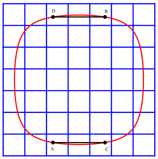
Figure 6: Level curve $\varphi(x,y)=h$.

Figure 7: Reflections of the square.

The level set $\varphi(x,y)=h$ is a simple closed curve as in Figure 7 with its interior $\varphi(x,y)>h$ being a strictly convex domain. Since $(k,\,l_{p})=(k,\,l_{q})=1$, there exist unique integers $L$, $M\in\{1,\dots,k-1\}$ coprime to $k$ such that $l_{q}\equiv Ll_{p}$ and $l_{p}\equiv Ml_{q}\mod k$. We can write

$$\alpha=l_{\alpha}/k+\alpha^{\prime},\qquad\beta=l_{\beta}/k+\beta^{\prime},\qquad l_{\alpha},\,l_{\beta}\in\mathbb{Z},\qquad 0<\alpha^{\prime},\,\beta^{\prime}<1/k,$$ (88)

where a priori the last condition should be $0\leq\alpha^{\prime},\,\beta^{\prime}<1/k$ but equality is ruled out by Claim 1. Let $i_{\alpha}\in\{0,\dots,k-1\}$ be the unique integer such that $i_{\alpha}\equiv l_{\alpha}-Ml_{\beta}\mod k$.

Claim 3. The $k$ points in (87) can be rearranged as

$$(i/k+\alpha^{\prime},\,\{L\,(i-i_{\alpha})/k+\beta^{\prime}\})\qquad(i=0,\dots,k-1).$$ (89)

Observe that $(\{pj+\alpha\},\,\{qj+\beta\})=(\{(l_{p}j+l_{\alpha})/k+\alpha^{\prime}\},\,\{(l_{q}j+l_{\beta})/k+\beta^{\prime}\})$. We work with the quotient ring $\mathbb{Z}/k\mathbb{Z}$ and its unit group $(\mathbb{Z}/k\mathbb{Z})^{\times}$. Note that $L=l_{q}l_{p}^{-1}$ and $M=L^{-1}=l_{p}l_{q}^{-1}$ in $(\mathbb{Z}/k\mathbb{Z})^{\times}$. If $i=l_{p}j+l_{\alpha}$ in $\mathbb{Z}/k\mathbb{Z}$ then $j=l_{p}^{-1}(i-l_{\alpha})$ and so $l_{q}j+l_{\beta}=l_{q}l_{p}^{-1}(i-l_{\alpha})+l_{\beta}=(l_{q}l_{p}^{-1})(i-l_{\alpha}+(l_{p}l_{q}^{-1})l_{\beta})=L(i-l_{\alpha}+Ml_{\beta})=L(i-i_{\alpha})$ in $\mathbb{Z}/k\mathbb{Z}$. Thus $(\{pj+\alpha\},\,\{qj+\beta\})$ $(j=0,\dots,k-1)$ can be rearranged as $(\{i/k+\alpha^{\prime}\},\,\{L(i-i_{\alpha})/k+\beta^{\prime}\})$ $(i=0,\dots,k-1)$. Since $\{i/k+\alpha^{\prime}\}=i/k+\alpha^{\prime}$ by $i=0,\dots,k-1$ and $0<\alpha^{\prime}<1/k$, we have formula (89). $\Box$

If the square $[0,\,1)\times[0,\,1)$ is equi-partitioned into $k$ columns and $k$ rows as in Figure 7, then rearrangement (89) tells us that each column contains exactly one point from (87), where the index $i$ in (89) corresponds to the $(i+1)$-th column of the square. Similarly, a row version of (89) implies that each row also contains exactly one point from (87). By Claim 1 each point of (87) must be in the interior of a small square (or a box) created by the $k$-by-$k$ partition.

Notice that the function $\varphi(x,y)$ is invariant under two reflections $r_{1}:(x,\,y)\mapsto(1-x,\,y)$ and $r_{2}:(x,\,y)\mapsto(x,\,1-y)$ (see Figure 7). On the other hand we have $1-\{t\}=\{-t\}$ whenever $t\in\mathbb{R}\setminus\mathbb{Z}$, which yields $1-\{pj+\alpha\}=\{-pj-\alpha\}$ and $1-\{qj+\beta\}=\{-qj-\beta\}$, since neither $pj+\alpha$ nor $qj+\beta$ is an integer by Claim 1. Thus these reflections induce two symmetries

$$r_{1}:(p,q;\alpha,\beta)\mapsto(-p,q;-\alpha,\beta),\qquad r_{2}:(p,q;\alpha,\beta)\mapsto(p,-q;\alpha,-\beta).$$ (90)

among solutions to our current problem, which may be settled only up to these symmetries.

Let $\mathrm{A}$ be the point from (87) that lie in the bottom row and $c_{\mathrm{A}}$ the column that contains $\mathrm{A}$. Similarly let $\mathrm{B}$ be the point from (87) that lie in the top row and $c_{\mathrm{B}}$ the column that contains $\mathrm{B}$ (see Figure 7). For two columns $c_{1}$ and $c_{2}$ we write $c_{1}\prec c_{2}$ if $c_{1}$ is located to the left of $c_{2}$. We may assume $c_{\mathrm{A}}\prec c_{\mathrm{B}}$, for otherwise $c_{\mathrm{A}}$ and $c_{\mathrm{B}}$ can be exchanged by the reflection $r_{1}$.

Claim 4. If $c_{\mathrm{A}}\prec c_{\mathrm{B}}$ then $c_{\mathrm{B}}$ must be the right neighbor of $c_{\mathrm{A}}$, $L=k-1$ in (89), and

$$l_{p}+l_{q}\equiv 0,\qquad l_{\alpha}+l_{\beta}\equiv i_{\alpha}\quad\mod k.$$ (91)

Suppose the contrary that there is an intermediate column $c$ between $c_{\mathrm{A}}$ and $c_{\mathrm{B}}$. Let $\mathrm{C}$ resp. $\mathrm{D}$ be the $r_{2}$-reflection of the point $\mathrm{B}$ resp. $\mathrm{A}$ (see Figure 7). Since the interior $\varphi(x,y)>h$ of the level curve $\varphi(x,y)=h$ is strictly convex, the level arc $\mathrm{A}\mathrm{C}$ is lower than the line segment $\mathrm{A}\mathrm{C}$ while the level arc $\mathrm{D}\mathrm{B}$ is upper than the line segment $\mathrm{D}\mathrm{B}$ (see Figure 7). Thus the level curve $\varphi(x,y)=h$ meets the column $c$ in its top and bottom boxes only. So the unique point from (87) lying in the column $c$ must be either in the top box or in the bottom box. But this is impossible because the top and bottom rows are already occupied by the points $\mathrm{B}$ and $\mathrm{A}$ respectively. Therefore the columns $c_{\mathrm{A}}$ and $c_{\mathrm{B}}$ must be consecutive, that is, $c_{\mathrm{B}}$ must be the right neighbor of $c_{\mathrm{A}}$ since $c_{\mathrm{A}}\prec c_{\mathrm{B}}$. Next we show that $L=k-1$. In view of formula (89) with $i=i_{\alpha}$ the point $\mathrm{A}$ has coordinates $(i_{\alpha}/k+\alpha^{\prime},\,\beta^{\prime})$, where $i_{\alpha}\in\{0,\dots,k-2\}$ because $c_{\mathrm{A}}$ is not the rightmost column. The point $\mathrm{B}$ is then given by formula (89) with $i=i_{\alpha}+1$, that is, by $((i_{\alpha}+1)/k+\alpha^{\prime},\,\{L/k+\beta^{\prime}\})$, where $\{L/k+\beta^{\prime}\}=L/k+\beta^{\prime}$ since $L\in\{1,\dots,k-1\}$ and $0<\beta^{\prime}<1/k$. In order for $\mathrm{B}$ to be in the top row, one must have $L=k-1$. Accordingly, $L\equiv M\equiv-1\mod k$ so that $l_{q}\equiv Ll_{p}\equiv-l_{p}$ and $i_{\alpha}\equiv l_{\alpha}-Ml_{\beta}\equiv l_{\alpha}+l_{\beta}\mod k$. $\Box$

Claim 5. The case $k\geq 5$ is impossible and so one has at most $k=3$, $4$.

Claim 4 and formula (89) show that if $c_{\mathrm{A}}\prec c_{\mathrm{B}}$ then the $k$ points in (87) are given by

$$\begin{cases}(i/k+\alpha^{\prime},\,(i_{\alpha}-i)/k+\beta^{\prime})&(i=0,\dots,i_{\alpha}),\\ (i/k+\alpha^{\prime},\,(i_{\alpha}-i)/k+\beta^{\prime}+1)&(i=i_{\alpha}+1,\dots,k-1),\end{cases}$$ (92)

which comprises two straight strings $\mathrm{A}^{\prime}\mathrm{A}$ and $\mathrm{B}\mathrm{B}^{\prime}$ of slope $-1$ as in Figure 8.

Figure 8: A configuration of the $k$ points (when $k=7$).

Each string cannot contain more than two points, because the interior $\varphi(x,y)>h$ of the level curve $\varphi(x,y)=h$ is strictly convex so that three collinear points cannot lie on the level curve. Thus if $k_{\mathrm{A}}$ resp. $k_{\mathrm{B}}$ stands for the number of points on the string $\mathrm{A}^{\prime}\mathrm{A}$ resp. $\mathrm{B}\mathrm{B}^{\prime}$, then one must have $k_{\mathrm{A}}\leq 2$ and $k_{\mathrm{B}}\leq 2$ so that $k=k_{\mathrm{A}}+k_{\mathrm{B}}\leq 4$. (Figure 8 exhibits a configuration that is impossible.) $\Box$

Note that $k_{\mathrm{A}}=i_{\alpha}+1$ since the point $\mathrm{A}$ belongs to the $(i_{\alpha}+1)$-th column. Observe that the transformation $r_{1}\circ r_{2}$ brings $\alpha^{\prime}\mapsto 1/k-\alpha^{\prime}$, $\beta^{\prime}\mapsto 1/k-\beta^{\prime}$ and $i_{\alpha}\mapsto k-2-i_{\alpha}$ without violating the condition $c_{\mathrm{A}}\prec c_{\mathrm{B}}$. So the symmetry allows us to assume $i_{\alpha}\leq k-2-i_{\alpha}$, that is, $0\leq i_{\alpha}\leq[k/2]-1$ in addition to $c_{\mathrm{A}}\prec c_{\mathrm{B}}$; when $k=3$ this means that we may assume $i_{\alpha}=0$.

Claim 6. When $k=3$, if $c_{\mathrm{A}}\prec c_{\mathrm{B}}$ and $i_{\alpha}=0$ then

$$p\in\frac{\varepsilon}{3}+\mathbb{Z},\quad p\in-\frac{\varepsilon}{3}+\mathbb{Z},\quad\alpha\in\frac{\delta}{3}+\kappa+\mathbb{Z},\quad\beta\in-\frac{\delta}{3}+\kappa+\mathbb{Z},$$ (93)

where $\varepsilon=\pm 1$, $\delta=0,\,\pm 1$ and $\kappa$ is the irrational constant defined by formula (84).

If $k=3$ and $i_{\alpha}=0$, the three points in formula (92) are given by $\mathrm{A}(\alpha^{\prime},\,\beta^{\prime})$, $\mathrm{B}(\alpha^{\prime}+1/3,\,\beta^{\prime}+2/3)$ and $\mathrm{B}^{\prime}(\alpha^{\prime}+2/3,\,\beta^{\prime}+1/3)$, where $0<\alpha^{\prime},\,\beta^{\prime}<1/3$. Condition (85) now reads

$$\sin\pi\alpha^{\prime}\cdot\sin\pi\beta^{\prime}=\sin\pi(\alpha^{\prime}+1/3)\cdot\sin\pi(\beta^{\prime}+2/3)=\sin\pi(\alpha^{\prime}+2/3)\cdot\sin\pi(\beta^{\prime}+1/3).$$

Addition formula for sine recasts the second equality to $\tan\pi\alpha^{\prime}=\tan\pi\beta^{\prime}$ and so $\alpha^{\prime}=\beta^{\prime}$. The first equality then becomes $\tan^{2}\pi\alpha^{\prime}=3/5$ yielding $\alpha^{\prime}=\beta^{\prime}=\frac{1}{\pi}\arctan\sqrt{3/5}$, which is the constant $\kappa$ defined by (84). The configuration of the three points is as in Figure 10. Formula (93) follows from $p=l_{p}/3$, $q=l_{q}/3$ with $(3,\,l_{p})=(3,\,l_{q})=1$ and formulas (88) and (91) with $i_{\alpha}=0$. $\Box$

Claim 7. When $k=4$, if $c_{\mathrm{A}}\prec c_{\mathrm{B}}$ then

$$p\in\frac{\varepsilon}{4}+\mathbb{Z},\quad q\in-\frac{\varepsilon}{4}+\mathbb{Z},\quad\alpha\in\frac{2+\delta}{8}+\mathbb{Z},\quad\beta\in\frac{2-\delta}{8}+\mathbb{Z}\quad(\varepsilon=\pm 1,\,\delta=\pm 1,\,\pm 3).$$ (94)

We must have $k_{\mathrm{A}}=k_{\mathrm{B}}=2$ and so $i_{\alpha}=1$, because $k_{\mathrm{A}}\leq 2$, $k_{\mathrm{B}}\leq 2$ and $k_{\mathrm{A}}+k_{\mathrm{B}}=k=4$. If $k=4$ and $i_{\alpha}=1$, the four points in (92) are given by $\mathrm{A}(\alpha^{\prime}+1/4,\,\beta^{\prime})$, $\mathrm{B}(\alpha^{\prime}+2/4,\,\beta^{\prime}+3/4)$, $\mathrm{A}^{\prime}(\alpha^{\prime},\,\beta^{\prime}+1/4)$ and $\mathrm{B}^{\prime}(\alpha^{\prime}+3/4,\,\beta^{\prime}+2/4)$, where $0<\alpha^{\prime},\,\beta^{\prime}<1/4$. Condition (85) now implies

$$\sin\pi\alpha^{\prime}\cdot\sin\pi(\beta^{\prime}+1/4)=\sin\pi(\alpha^{\prime}+1/4)\cdot\sin\pi\beta^{\prime}=\sin\pi(\alpha^{\prime}+2/4)\cdot\sin\pi(\beta^{\prime}+3/4),$$

where the first equality comes from $\varphi(\mathrm{A}^{\prime})=\varphi(\mathrm{A})$ while the second one from $\varphi(\mathrm{A})=\varphi(\mathrm{B})$. Addition formula for sine recasts the first equality to $\tan\pi\alpha^{\prime}=\tan\pi\beta^{\prime}$ and so $\alpha^{\prime}=\beta^{\prime}$. The second equality then becomes $\tan 2\pi\alpha^{\prime}=1$ yielding $\alpha^{\prime}=\beta^{\prime}=1/8$.

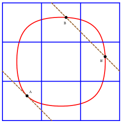
Figure 9: $k=3$.

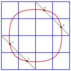
Figure 10: $k=4$.

The configuration of the four points is indicated in Figure 10. Formula (94) follows from $p=l_{p}/4$, $q=l_{q}/4$ with $(4,\,l_{p})=(4,\,l_{q})=1$ and formulas (88) and (91) with $i_{\alpha}=1$. $\Box$

We are now in a position to establish cases (6) and (7) of Proposition 9.2. Replace $\delta$ by $\varepsilon\delta$ in the third and fourth formulas in (93). Using $\mathbb{Z}_{2}\times\mathbb{Z}_{2}$ symmetries in (90), multiply the first and third formulas by $\varepsilon_{p}\varepsilon$, while the second and fourth formulas by $-\varepsilon_{q}\varepsilon$, where $\varepsilon_{p},\varepsilon_{q}=\pm 1$. We then arrive at case (6). Similarly, replace $\delta$ by $\varepsilon\delta$ in the third and fourth formulas in (94). Multiply the first and third formulas by $\varepsilon_{p}\varepsilon$, while the second and fourth formulas by $-\varepsilon_{q}\varepsilon$, where $\varepsilon_{p}$, $\varepsilon_{q}=\pm 1$. We then arrive at case (7). The proof of Proposition 9.2 is complete. $\Box$

10 Parity

Proposition 8.1 was able to confine the possibilities of $(p,q;\alpha,\beta)$ substantially as in Proposition 9.2. We shall discuss how further Proposition 8.2 can reduce those possibilities.

Lemma 10.1

Let $r\in\mathbb{N}$, $p\in\mathbb{Q}^{\times}$ and $\alpha\in\mathbb{R}$. The sequence $\sin\pi\{pj+\alpha\}$ takes a nonzero constant value and the integer sequence $[pj+\alpha]+rj$ has a constant parity independent of $j\in\mathbb{Z}$, if and only if $p$ is an integer with the same parity as $r$ and $\alpha\in\mathbb{R}\setminus\mathbb{Z}$.

Proof. We are either in case (1) or in case (2) of Lemma 9.1. We begin by case (1). We must have $\alpha\in\mathbb{R}\setminus\mathbb{Z}$ because $\sin\pi\{\alpha\}$ should be nonzero. Since $p\in\mathbb{Z}$ we have $[pj+\alpha]+rj=(p+r)j+[\alpha]$, which has a constant parity if and only if $p+r$ is even, that is, $p$ and $r$ have the same parity. We proceed to case (2). Note that $2p$ is an odd integer since $p\in 1/2+\mathbb{Z}$. Replacing $j$ by $2j$ we have $[2pj+\alpha]+2rj=(2p+2r)j+[\alpha]\equiv j+[\alpha]\mod 2$ since $2p$ is odd and $2r$ is even. Clearly $j+[\alpha]$ cannot have a constant parity, so that case (2) must be ruled out. $\Box$

Proposition 10.2

Let $r\in\mathbb{N}$, $p,\,q\in\mathbb{Q}^{\times}$ and $\alpha,\,\beta\in\mathbb{R}$. The sequence $\sin\pi\{pj+\alpha\}\cdot\sin\pi\{qj+\beta\}$ takes a nonzero constant value and the integer sequence $[pj+\alpha]+[qj+\beta]+rj$ has a constant parity independent of $j\in\mathbb{Z}$, if and only if either condition $(\mathrm{A})$ or $(\mathrm{B})$ below is satisfied:

1. $p,\,q\in\mathbb{Z}$, $p+q+r$ is even, and $\alpha,\,\beta\in\mathbb{R}\setminus\mathbb{Z}$.

2. $p,\,q\in 1/2+\mathbb{Z}$, $\alpha,\,\beta\in\mathbb{R}\setminus\mathbb{Z}$, and $\alpha-(-1)^{p+q+r}\beta\in 1/2+\mathbb{Z}$.

Proof. We are in one of seven cases (1)–(7) of Proposition 9.2, but case (1) is ruled out because the constant $\sin\pi\{\alpha\}\cdot\sin\pi\{\beta\}$ vanishes in this case. We shall make a case-by-case check as to whether the sequence $[pj+\alpha]+[qj+\beta]+rj$ can have a constant parity. In case (2), since $p$ and $q$ are integers, we have $[pj+\alpha]+[qj+\beta]+rj=(p+q+r)j+[\alpha]+[\beta]$, which has a constant parity if and only if $p+q+r$ is even. This is just the case of type $(\mathrm{A})$ in Proposition 10.2. Next we consider case (3) where $p\in\mathbb{Z}$ and $q\in 1/2+\mathbb{Z}$. Replacing $j$ by $2j$ in $[pj+\alpha]+[qj+\beta]+rj$ we have $[2pj+\alpha]+[2qj+\beta]+2rj=(2p+2q+2r)j+[\alpha]+[\beta]\equiv j+[\alpha]+[\beta]\mod 2$, since $2p$ and $2r$ are even while $2q$ is odd. Clearly $j+[\alpha]+[\beta]$ cannot have a constant parity, so that case (3) must be ruled out. For the same reason case (4) is also ruled out.

We turn our attention to case (5). Since $p,\,q\in 1/2+\mathbb{Z}$, observe that $2p$ and $2q$ are odd integers and so $2p+2q$ is an even integer. Putting $j=2k+l$ with $k\in\mathbb{Z}$ and $l=0,1$, we have $[pj+\alpha]+[qj+\beta]+rj=[2pk+pl+\alpha]+[2qk+ql+\beta]+2rk+rl=(2p+2q+2r)k+[pl+\alpha]+[ql+\beta]+rl\equiv[pl+\alpha]+[ql+\beta]+rl\mod 2$ for every $k\in\mathbb{Z}$. So the sequence $[pj+\alpha]+[qj+\beta]+rj$ has a constant parity if and only if $[\alpha]+[\beta]\equiv[p+\alpha]+[q+\beta]+r\mod 2$, which is equivalent to

$$[p]+[q]+r\equiv[1/2+\{\alpha\}]+[1/2+\{\beta\}]\mod 2,$$ (95)

because $[p+\alpha]+[q+\beta]=[p]+[\alpha]+[1/2+\{\alpha\}]+[q]+[\beta]+[1/2+\{\beta\}]$. In case (5) we have either $\alpha+\beta\in 1/2+\mathbb{Z}$ or $\alpha-\beta\in 1/2+\mathbb{Z}$, where the former condition implies (i) $\{\alpha\}+\{\beta\}=1/2$ or (ii) $\{\alpha\}+\{\beta\}=3/2$, while the latter implies (iii) $\{\alpha\}-\{\beta\}=1/2$ or (iv) $\{\beta\}-\{\alpha\}=1/2$. Note that $\{\alpha\}$ and $\{\beta\}$ must be positive, that is, $\alpha$, $\beta\in\mathbb{R}\setminus\mathbb{Z}$, since $\sin\pi\{\alpha\}\cdot\sin\pi\{\beta\}$ is nonzero. So $[1/2+\{\alpha\}]=[1/2+\{\beta\}]=0$ in subcase (i); $[1/2+\{\alpha\}]=[1/2+\{\beta\}]=1$ in subcase (ii); $[1/2+\{\alpha\}]=1$, $[1/2+\{\beta\}]=0$ in subcase (iii); $[1/2+\{\alpha\}]=0$, $[1/2+\{\beta\}]=1$ in subcase (iv). Thus condition (95) becomes $[p]+[q]+r\equiv 0\mod 2$ in subcases (i) and (ii); and $[p]+[q]+r\equiv 1\mod 2$ in subcases (iii) and (iv). This shows that $p+q+r$ is odd if $\alpha+\beta\in 1/2+\mathbb{Z}$; and even if $\alpha-\beta\in 1/2+\mathbb{Z}$, since $p+q=(1/2+[p])+(1/2+[q])=[p]+[q]+1$. In either case we have $\alpha-(-1)^{p+q+r}\beta\in 1/2+\mathbb{Z}$, so that we are led to the case of type $(\mathrm{B})$ in Proposition 10.2.

We proceed to case (6). In this case $p=\varepsilon_{p}/3+p^{\prime}$ and $q=\varepsilon_{q}/3+q^{\prime}$ with some $\varepsilon_{p},\,\varepsilon_{q}=\pm 1$ and $p^{\prime},\,q^{\prime}\in\mathbb{Z}$. Note that $\varepsilon_{p}+\varepsilon_{q}$ is even in every choice of $\varepsilon_{p}$ and $\varepsilon_{q}$. Putting $j=3k+l$ with $k\in\mathbb{Z}$ and $l=0,\pm 1$, we have $[pj+\alpha]+[qj+\beta]+rj=(\varepsilon_{p}+\varepsilon_{q}+3p^{\prime}+3q^{\prime}+3r)k+[lp+\alpha]+[lq+\beta]+lr\equiv(p^{\prime}+q^{\prime}+r)k+[pl+\alpha]+[ql+\beta]+rl\mod 2$. In order for this to have a common parity for every $k\in\mathbb{Z}$ the integer $p^{\prime}+q^{\prime}+r$ must be even. Under this condition, $[p+\alpha]+[q+\beta]+r=p^{\prime}+q^{\prime}+r+[\varepsilon_{p}/3+\alpha]+[\varepsilon_{q}/3+\beta]\equiv[\varepsilon_{p}/3+\alpha]+[\varepsilon_{q}/3+\beta]\mod 2$ and $[-p+\alpha]+[-q+\beta]-r=-(p^{\prime}+q^{\prime}+r)+[-\varepsilon_{p}/3+\alpha]+[-\varepsilon_{q}/3+\beta]\equiv[-\varepsilon_{p}/3+\alpha]+[-\varepsilon_{q}/3+\beta]\mod 2$. Thus the parity of $[pl+\alpha]+[ql+\beta]+rl$ being constant for $l=0,\pm 1$ means

$$[\alpha]+[\beta]\equiv[\varepsilon_{p}/3+\alpha]+[\varepsilon_{q}/3+\beta]\equiv[-\varepsilon_{p}/3+\alpha]+[-\varepsilon_{q}/3+\beta]\mod 2.$$

Since $\alpha\in\varepsilon_{p}(\delta/3+\varepsilon\kappa)+\mathbb{Z}$ and $\beta\in\varepsilon_{q}(\delta/3-\varepsilon\kappa)+\mathbb{Z}$ with $\varepsilon=\pm 1$, $\delta=0,\pm 1$, this becomes

$$\textstyle[\varepsilon_{p}(\frac{\delta}{3}+\varepsilon\kappa)]+[\varepsilon_{q}(\frac{\delta}{3}-\varepsilon\kappa)]\equiv[\varepsilon_{p}(\frac{\delta+1}{3}+\varepsilon\kappa)]+[\varepsilon_{q}(\frac{\delta+1}{3}-\varepsilon\kappa)]\equiv[\varepsilon_{p}(\frac{\delta-1}{3}+\varepsilon\kappa)]+[\varepsilon_{q}(\frac{\delta-1}{3}-\varepsilon\kappa)].$$

Note that if $t$ is not an integer then $[-t]=-[t]-1\equiv[t]+1\mod 2$ and hence $[\epsilon t]\equiv[t]+\frac{1-\epsilon}{2}\mod 2$ for $\epsilon=\pm 1$. This rule allows us to remove $\varepsilon_{p}$ and $\varepsilon_{q}$ from the above condition, that is,

$$\textstyle[\frac{\delta}{3}+\kappa]+[\frac{\delta}{3}-\kappa]\equiv[\frac{\delta+1}{3}+\kappa]+[\frac{\delta+1}{3}-\kappa]\equiv[\frac{\delta-1}{3}+\kappa]+[\frac{\delta-1}{3}-\kappa]\mod 2,$$ (96)

where $\varepsilon$ can also be removed by symmetry. Since $\kappa=0.209785\cdots$ in formula (84), congruences (96) become $-1\equiv 0\equiv-2$ if $\delta=0$; $0\equiv 0\equiv-1$ if $\delta=1$; and $-2\equiv-1\equiv-2$ if $\delta=-1$, respectively. In any case we have a contradiction and thus case (6) is ruled out.

Finally we consider case (7). In this case $p=\varepsilon_{p}/4+p^{\prime}$ and $q=\varepsilon_{q}/4+q^{\prime}$ with some $\varepsilon_{p},\,\varepsilon_{q}=\pm 1$ and $p^{\prime},\,q^{\prime}\in\mathbb{Z}$. The parity of $[pj+\alpha]+[qj+\beta]+rj$ being equal for $j=0,2$ yields $[\alpha]+[\beta]\equiv[2p+\alpha]+[2q+\beta]+2r=[\varepsilon_{p}/2+\alpha]+[\varepsilon_{q}/2+\beta]+2(p^{\prime}+q^{\prime}+r)\equiv[\varepsilon_{p}/2+\alpha]+[\varepsilon_{q}/2+\beta]\mod 2$. Since $\alpha\in\varepsilon_{p}(\delta/8+\varepsilon/4)+\mathbb{Z}$ and $\beta\in\varepsilon_{q}(\delta/8-\varepsilon/4)+\mathbb{Z}$ with $\varepsilon=\pm 1$ and $\delta=\pm 1,\pm 3$,

$$\textstyle[\varepsilon_{p}(\frac{\delta}{8}+\frac{\varepsilon}{4})]+[\varepsilon_{q}(\frac{\delta}{8}-\frac{\varepsilon}{4})]\equiv[\varepsilon_{p}(\frac{\delta}{8}+\frac{\varepsilon}{4}+\frac{1}{2})]+[\varepsilon_{q}(\frac{\delta}{8}-\frac{\varepsilon}{4}+\frac{1}{2})]\mod 2.$$

For the same reason as in the last paragraph, $\varepsilon_{p}$ and $\varepsilon_{q}$ can be removed from the above condition:

$$\textstyle[\frac{\delta}{8}+\frac{1}{4}]+[\frac{\delta}{8}-\frac{1}{4}]\equiv[\frac{\delta}{8}+\frac{1}{4}+\frac{1}{2}]+[\frac{\delta}{8}-\frac{1}{4}+\frac{1}{2}]\mod 2,$$

where $\varepsilon$ can also be removed by symmetry. But the right-hand side above is $[\frac{\delta}{8}+\frac{3}{4}]+[\frac{\delta}{8}+\frac{1}{4}]=[\frac{\delta}{8}+\frac{1}{4}]+[\frac{\delta}{8}-\frac{1}{4}]+1$, which leads to a contradiction $0\equiv 1\mod 2$. Thus case (7) is ruled out. $\Box$

Note that Theorem 2.4 follows from Propositions 8.1, 8.2, 10.2 and Lemma 8.3.

11 The Method of Contiguous Relations

If $p$, $q$, $r$ are integers then contiguous relations of Gauss lead to a general three-term relation (5) and a specialization (7) of it evaluated at $(\alpha,\beta;\gamma;z)=(pw+a,qw+b;rw;x)$. In this section we shall see how these formulas contribute to the discussions of Problems 1.4 and 2.2.

11.1 Rational Independence

To settle Problem 1.4 in region (8) and prove Theorem 2.7, we begin by the following.

Lemma 11.1

If $\lambda=(p,q,r;a,b;x)$ is a non-elementary solution to Problem 1.2 in region (8), then $f(w)$ and $\tilde{f}(w)$ in (1) and (6)are linearly independent over the rational function field $\mathbb{C}(w)$.

Proof. If $\gamma$ is not an integer then the Gauss hypergeometric equation admits

$$u_{1}:={}_{2}F_{1}(\alpha,\beta;\gamma;z),\quad u_{2}:=z^{1-\gamma}{}_{2}F_{1}(\alpha-\gamma+1,\beta-\gamma+1;2-\gamma;z)$$

as a fundamental set of solutions, whose Wronskian is given by

$$W:=u_{1}u_{2}^{\prime}-u_{1}^{\prime}u_{2}=(1-\gamma)z^{-\gamma}(1-z)^{\gamma-\alpha-\beta-1},$$

where $u^{\prime}=du/dz$. From formulas (20) and (22) of Erdélyi [8, Chapter II, §2.8],

$$u_{1}^{\prime}=\frac{\alpha\beta}{\gamma}\,{}_{2}F_{1}(\alpha+1,\beta+1;\gamma+1;z),\quad u_{2}^{\prime}=(1-\gamma)z^{-\gamma}\,{}_{2}F_{1}(\alpha-\gamma+1,\beta-\gamma+1;1-\gamma;z).$$

Substituting these into the Wronskian formula above one has

$$\begin{split}&(1-z)^{\gamma-\alpha-\beta-1}={}_{2}F_{1}(\alpha,\beta;\gamma;z)\,{}_{2}F_{1}(\alpha-\gamma+1,\beta-\gamma+1;1-\gamma;z)+\\ &\frac{\alpha\beta z}{\gamma(\gamma-1)}\,{}_{2}F_{1}(\alpha+1,\beta+1;\gamma+1;z)\,{}_{2}F_{1}(\alpha-\gamma+1,\beta-\gamma+1;2-\gamma;z).\end{split}$$ (97)

Since $\lambda$ is a non-elementary solution to Problem 1.2, $f(w)$ has a GPF (57) with $m\geq 1$ by Propositions 5.4 and 6.2. If $f(w)$ and $\tilde{f}(w)$ were linearly dependent over $\mathbb{C}(w)$, then there would be a rational function $T(w)$ such that $\tilde{f}(w)=T(w)f(w)$. Putting $\alpha=pw+a$, $\beta=qw+b$, $\gamma=rw$ and $z=x$ into formula (97) yields $f(w)f_{1}(w)=(1-x)^{(r-p-q)w-a-b-1}$, where

$$f_{1}(w) :={}_{2}F_{1}((p-r)w+a+1,\,(q-r)w+b+1;\,1-rw;\,x)$$

$$\quad+\frac{(pw+a)(qw+b)x}{rw(rw-1)}\cdot T(w)\cdot{}_{2}F_{1}((p-r)w+a+1,\,(q-r)w+b+1;\,2-rw;\,x).$$

Take a negative real number $R_{5}$ so that all poles of $T(w)$ and $S(w)$ are in the right half-plane $\mathrm{Re}(z)>R_{5}$, where $S(w)$ is the rational function in formula (57). Since $r$ is positive, $f_{1}(w)$ is holomorphic on the left half-plane $\mathrm{Re}(z)<R_{5}$. Choose a positive integer $j$ so that $-j-v_{1}<R_{5}$. Then $f(w)$ has a zero at $w=-j-v_{1}$ while $f_{1}(w)$ is holomorphic at this point. Therefore, $0=f(-j-v_{1})f_{1}(-j-v_{1})=(1-x)^{-(r-p-q)(j+v_{1})-a-b-1}\neq 0$, which is a contradiction. $\Box$

Proposition 11.2

If $\lambda=(p,q,r;a,b,x)$ is a non-elementary solution to Problem 1.2 in region (8) with $p,q,r\in\mathbb{Z}$, then it comes from contiguous relations. In particular Theorem 2.7 holds.

Proof. Since $\lambda$ is a solution to Problem 1.2, there exists a rational function $\widetilde{R}(w)$ such that $f(w+1)=\widetilde{R}(w)f(w)$. Subtracting this from three-term relation (7) yields a linear relation $\{R(w)-\widetilde{R}(w)\}f(w)+Q(w)\tilde{f}(w)=0$ over $\mathbb{C}(w)$. By Lemma 11.1 one must have $R(w)-\widetilde{R}(w)=Q(w)=0$ in $\mathbb{C}(w)$, so that three-term relation (7) degenerates to a two-term one (3). $\Box$

11.2 Contiguous Relations in Matrix Form

It is convenient to rewrite contiguous relations in a matrix form by putting

$$\mbox{\boldmath$F$}(\mbox{\boldmath$a$}):={}^{t}({}_{2}F_{1}(\mbox{\boldmath$a$};z),\,{}_{2}F_{1}(\mbox{\boldmath$a$}+\mbox{\boldmath$1$};z)),\qquad\mbox{\boldmath$a$}:=(a_{1},a_{2};a_{3})=(\alpha,\beta;\gamma),\quad\mbox{\boldmath$1$}:=(1,1;1),$$

and $\mbox{\boldmath$e$}_{1}=(1,0;0)$, $\mbox{\boldmath$e$}_{2}=(0,1;0)$, $\mbox{\boldmath$e$}_{3}=(0,0;1)$. From formulas in Erdélyi [8, Chapter II, §2.8], we observe that the contiguous relation raising parameter $a_{i}$ by one can be written

$$\mbox{\boldmath$F$}(\mbox{\boldmath$a$}+\mbox{\boldmath$e$}_{i})=A_{i}(\mbox{\boldmath$a$})\,\mbox{\boldmath$F$}(\mbox{\boldmath$a$})\qquad(i=1,2,3),$$ (98)

where the matrix $A_{i}(\mbox{\boldmath$a$})$ is given in Table 5, together with its determinant $\det A_{i}(\mbox{\boldmath$a$})$.

$$A_{1}(\mbox{\boldmath$a$}) :=\begin{pmatrix}1&\dfrac{\beta z}{\gamma}\\[11.38109pt] -\dfrac{\gamma}{(\alpha+1)(z-1)}&\dfrac{\gamma-\alpha-1-\beta z}{(\alpha+1)(z-1)}\end{pmatrix}, \det A_{1}(\mbox{\boldmath$a$}) =\dfrac{\gamma-\alpha-1}{(\alpha+1)(z-1)},$$

$$A_{2}(\mbox{\boldmath$a$}) :=\begin{pmatrix}1&\dfrac{\alpha z}{\gamma}\\[11.38109pt] -\dfrac{\gamma}{(\beta+1)(z-1)}&\dfrac{\gamma-\beta-1-\alpha z}{(\beta+1)(z-1)}\end{pmatrix}, \det A_{2}(\mbox{\boldmath$a$}) =\dfrac{\gamma-\beta-1}{(\beta+1)(z-1)},$$

$$A_{3}(\mbox{\boldmath$a$}) :=\begin{pmatrix}\dfrac{\gamma(\gamma-\alpha-\beta)}{(\gamma-\alpha)(\gamma-\beta)}&-\dfrac{\alpha\beta(z-1)}{(\gamma-\alpha)(\gamma-\beta)}\\[14.22636pt] \dfrac{\gamma(\gamma+1)}{(\gamma-\alpha)(\gamma-\beta)z}&\dfrac{\gamma(\gamma+1)(z-1)}{(\gamma-\alpha)(\gamma-\beta)z}\end{pmatrix}, \det A_{3}(\mbox{\boldmath$a$}) =\dfrac{\gamma(\gamma+1)(z-1)}{(\gamma-\alpha)(\gamma-\beta)z}.$$

Table 5: Contiguous matrices and their determinants.

As the compatibility conditions for three relations (98) one has the commutation relations:

$$A_{i}(\mbox{\boldmath$a$}+\mbox{\boldmath$e$}_{j})\,A_{j}(\mbox{\boldmath$a$})=A_{j}(\mbox{\boldmath$a$}+\mbox{\boldmath$e$}_{i})\,A_{i}(\mbox{\boldmath$a$})\qquad(i,j=1,2,3).$$ (99)

Given a lattice point $\mbox{\boldmath$p$}=(p_{1},p_{2};p_{3})=(p,q;r)\in\mathbb{Z}^{3}_{\geq 0}$, a lattice path in $\mathbb{Z}^{3}_{\geq 0}$ from $\mbox{\boldmath$0$}=(0,0;0)$ to $p$ can be represented by a sequence $i=(i_{1},\dots,i_{k})$ of indexes in $\{1,2,3\}$ such that $\mbox{\boldmath$p$}=\mbox{\boldmath$e$}_{i_{1}}+\cdots+\mbox{\boldmath$e$}_{i_{k}}$ where $k=p+q+r$. By compatibility conditions (99) the matrix product

$$A(\mbox{\boldmath$a$};\mbox{\boldmath$p$}):=A_{i_{k}}(\mbox{\boldmath$a$}+\mbox{\boldmath$e$}_{i_{1}}+\cdots+\mbox{\boldmath$e$}_{i_{k-1}})\cdots A_{i_{3}}(\mbox{\boldmath$a$}+\mbox{\boldmath$e$}_{i_{1}}+\mbox{\boldmath$e$}_{i_{2}})\,A_{i_{2}}(\mbox{\boldmath$a$}+\mbox{\boldmath$e$}_{i_{1}})\,A_{i_{1}}(\mbox{\boldmath$a$})$$

is independent of the path $i=(i_{1},\dots,i_{k})$, that is, depends only on the initial point $a$ and the terminal point $\mbox{\boldmath$a$}+\mbox{\boldmath$p$}$. The matrix version of three-term relation (5) is expressed as

$$\mbox{\boldmath$F$}(\mbox{\boldmath$a$}+\mbox{\boldmath$p$})=A(\mbox{\boldmath$a$};\mbox{\boldmath$p$})\,\mbox{\boldmath$F$}(\mbox{\boldmath$a$}).$$ (100)

Lemma 11.3

If $1\leq p\leq r$ and $1\leq q\leq r$ then $A(\mbox{\boldmath$a$};\mbox{\boldmath$p$})$ in (100) admits a representation

$$A(\mbox{\boldmath$a$};\mbox{\boldmath$p$})=\dfrac{1}{(\gamma-\alpha)_{r-p}\,(\gamma-\beta)_{r-q}}\begin{pmatrix}\dfrac{(\gamma)_{r}\,\phi_{11}^{(r-2)}}{(\alpha+1)_{p-1}\,(\beta+1)_{q-1}}&\dfrac{(\gamma+1)_{r-1}\,\phi_{12}^{(r-1)}}{(\alpha+1)_{p-1}\,(\beta+1)_{q-1}}\\[17.07164pt] \dfrac{(\gamma)_{r+1}\,\phi_{21}^{(r-1)}}{(\alpha+1)_{p}\,(\beta+1)_{q}}&\dfrac{(\gamma+1)_{r}\,\phi_{22}^{(r)}}{(\alpha+1)_{p}\,(\beta+1)_{q}}\end{pmatrix},$$ (101)

where $\phi_{11}^{(-1)}=0$ and $\phi_{ij}^{(k)}=\phi_{ij}^{(k)}(\mbox{\boldmath$a$};\mbox{\boldmath$p$})$ is a polynomial of degree at most $k$ in $\mbox{\boldmath$a$}=(\alpha,\beta;\gamma)$ with coefficients in the ring $\mathbb{Z}[z^{\pm 1},1/(z-1)]$. Moreover the determinant of $A(\mbox{\boldmath$a$};\mbox{\boldmath$p$})$ is given by

$$\det A(\mbox{\boldmath$a$};\mbox{\boldmath$p$})=\dfrac{z^{-r}(z-1)^{r-p-q}\cdot(\gamma)_{r}\,(\gamma+1)_{r}}{(\alpha+1)_{p}\,(\beta+1)_{q}\,(\gamma-\alpha)_{r-p}\,(\gamma-\beta)_{r-q}}.$$ (102)

Proof. Formula (101) is proved by induction on $r$, where the main claim is the assertion about the degrees of $\phi_{ij}^{(r)}$, $i,j=1,2$, in $\mbox{\boldmath$a$}=(\alpha,\beta;\gamma)$. A direct check shows that it is true for $r=1$, that is, for $\mbox{\boldmath$p$}=\mbox{\boldmath$1$}$. Assuming the assertion is true for $r$ we show it for $r+1$, that is, for $(p,q;r+1)$ with $1\leq p\leq r+1$ and $1\leq q\leq r+1$, where symmetry allows us to assume $p\leq q$. There are three cases to deal with: (i) $p\leq q\leq r$; (ii) $p<q=r+1$; and (iii) $p=q=r+1$. In case (i) the relation $A(\mbox{\boldmath$a$};\mbox{\boldmath$p$}+\mbox{\boldmath$e$}_{3})=A_{3}(\mbox{\boldmath$a$}+\mbox{\boldmath$p$})\,A(\mbox{\boldmath$a$};\mbox{\boldmath$p$})$ with $\mbox{\boldmath$p$}=(p,q;r)$ leads to the recurrence

$$\begin{pmatrix}\phi_{11}^{(r-1)}&\phi_{12}^{(r)\phantom{+1}}\\[5.69054pt] \phi_{21}^{(r)\phantom{-1}}&\phi_{22}^{(r+1)}\end{pmatrix}=\begin{pmatrix}\gamma-\alpha-\beta+r-p-q&1-z\\[5.69054pt] \dfrac{(\alpha+p)(\beta+q)}{z}&\dfrac{(\gamma+r)(z-1)}{z}\end{pmatrix}\begin{pmatrix}\phi_{11}^{(r-2)}&\phi_{12}^{(r-1)}\\[5.69054pt] \phi_{21}^{(r-1)}&\phi_{22}^{(r)\phantom{-1}}\end{pmatrix},$$

by which the assertion for $r+1$ follows from induction hypothesis. In case (ii) the relation $A(\mbox{\boldmath$a$};\mbox{\boldmath$p$}+\mbox{\boldmath$e$}_{2}+\mbox{\boldmath$e$}_{3})=A_{2}(\mbox{\boldmath$a$}+\mbox{\boldmath$p$}+\mbox{\boldmath$e$}_{3})\,A_{3}(\mbox{\boldmath$a$}+\mbox{\boldmath$p$})\,A(\mbox{\boldmath$a$};\mbox{\boldmath$p$})$ with $\mbox{\boldmath$p$}=(p,r;r)$ leads to

$$\begin{pmatrix}\phi_{11}^{(r-1)}&\phi_{12}^{(r)\phantom{+1}}\\[5.69054pt] \phi_{21}^{(r)\phantom{-1}}&\phi_{22}^{(r+1)}\end{pmatrix}=\begin{pmatrix}\beta+r&z-1\\[5.69054pt] -\dfrac{(\alpha+p)(\beta+r)}{z}&\dfrac{\gamma+r-(\alpha+p)z}{z}\end{pmatrix}\begin{pmatrix}\phi_{11}^{(r-2)}&\phi_{12}^{(r-1)}\\[5.69054pt] \phi_{21}^{(r-1)}&\phi_{22}^{(r)\phantom{-1}}\end{pmatrix},$$

by which the assertion follows from induction hypothesis. Finally, in case (iii) the relation $A(\mbox{\boldmath$a$};\mbox{\boldmath$p$}+\mbox{\boldmath$1$})=A_{1}(\mbox{\boldmath$a$}+\mbox{\boldmath$p$}+\mbox{\boldmath$e$}_{2}+\mbox{\boldmath$e$}_{3})\,A_{2}(\mbox{\boldmath$a$}+\mbox{\boldmath$p$}+\mbox{\boldmath$e$}_{3})\,A_{3}(\mbox{\boldmath$a$}+\mbox{\boldmath$p$})\,A(\mbox{\boldmath$a$};\mbox{\boldmath$p$})$ with $\mbox{\boldmath$p$}=(r,r;r)$ yields

$$\begin{pmatrix}\phi_{11}^{(r-1)}&\phi_{12}^{(r)\phantom{+1}}\\[5.69054pt] \phi_{21}^{(r)\phantom{-1}}&\phi_{22}^{(r+1)}\end{pmatrix}=\begin{pmatrix}0&1\\[11.38109pt] \dfrac{(\alpha+r)(\beta+r)}{z(1-z)}&\dfrac{\gamma+r-(\alpha+\beta+2r+1)z}{z(z-1)}\end{pmatrix}\begin{pmatrix}\phi_{11}^{(r-2)}&\phi_{12}^{(r-1)}\\[5.69054pt] \phi_{21}^{(r-1)}&\phi_{22}^{(r)\phantom{-1}}\end{pmatrix},$$

by which the assertion follows and the induction completes itself.

Determinant formula (102) is obtained by taking the determinant of matrix products

$$A(\mbox{\boldmath$a$};\mbox{\boldmath$p$}) =A_{1}(\alpha+p-1,\beta+q;\gamma+r)\cdots A_{1}(\alpha+1,\beta+q;\gamma+r)\,A_{1}(\alpha,\beta+q;\gamma+r)$$

$$\qquad\cdot A_{2}(\alpha,\beta+q-1;\gamma+r)\cdots A_{2}(\alpha,\beta+1;\gamma+r)\,A_{2}(\alpha,\beta;\gamma+r)$$ (103)

$$\qquad\cdot A_{3}(\alpha,\beta;\gamma+r-1)\cdots A_{3}(\alpha,\beta;\gamma+1)\,A_{3}(\alpha,\beta;\gamma),$$

and by using determinant formulas in Table 5. $\Box$

Lemma 11.3 readily leads to a matrix version of three-term relation (7):

$$\mbox{\boldmath$f$}(w+1)=A(w)\mbox{\boldmath$f$}(w),\qquad\mbox{\boldmath$f$}(w):={}^{t}(f(w),\tilde{f}(w)),$$ (104)

where the matrix $A(w)$ is described by Corollary 11.4 below. Note that the $(1,1)$-entry and $(1,2)$-entry of $A(w)$ are just $R(w)$ and $Q(w)$ in formula (7) respectively.

Corollary 11.4

If $1\leq p\leq r$ and $1\leq q\leq r$ then $A(w)$ in (104) admits a representation

$$\begin{split}A(w)&=\dfrac{1}{((r-p)w-a)_{r-p}\,((r-q)w-b)_{r-q}}\\[5.69054pt] &\times\begin{pmatrix}\dfrac{(rw)_{r}\,\phi_{11}^{(r-2)}(w)}{(pw+a+1)_{p-1}\,(qw+b+1)_{q-1}}&\dfrac{(rw+1)_{r-1}\,\phi_{12}^{(r-1)}(w)}{(pw+a+1)_{p-1}\,(qw+b+1)_{q-1}}\\[17.07164pt] \dfrac{(rw)_{r+1}\,\phi_{21}^{(r-1)}(w)}{(pw+a+1)_{p}\,(qw+b+1)_{q}}&\dfrac{(rw+1)_{r}\,\phi_{22}^{(r)}(w)}{(pw+a+1)_{p}\,(qw+b+1)_{q}}\end{pmatrix},\end{split}$$ (105)

where $\phi_{11}^{(-1)}(w)=0$ and $\phi_{ij}^{(k)}(w)$ is a polynomial of degree at most $k$ in $w$. Moreover,

$$\det A(w)=\dfrac{x^{-r}(x-1)^{r-p-q}\cdot(rw)_{r}\,(rw+1)_{r}}{(pw+a+1)_{p}\,(qw+b+1)_{q}\,((r-p)w-a)_{r-p}\,((r-q)w-b)_{r-q}}.$$ (106)

Proof. In view of (100), substitute $\mbox{\boldmath$a$}=\mbox{\boldmath$\alpha$}(w):=(pw+a,qw+b;rw)$ and $z=x$ into (101). $\Box$

Remark 11.5

In three-term relation (7) we have $Q(w)=A_{12}(w)$ and $R(w)=A_{11}(w)$ evaluated at $z=x$, where $A_{ij}(w)$ denotes the $(i,j)$-th entry of the matrix $A(w)$. Thus a solution $\lambda=(p,q,r;a,b;x)$ to Problem 1.2 comes from contiguous relations exactly when $A_{12}(w)$ or equivalently $\phi_{12}^{(r-1)}(w)$ vanishes in $\mathbb{C}(w)$ (upon putting $z=x$). If this is the case, then taking the determinant of formula (105) and comparing the result with formula (106), we find

$$\phi_{11}^{(r-2)}(w)\cdot\phi_{22}^{(r)}(w)=x^{-r}(x-1)^{r-p-q}\cdot(pw+a+1)_{p-1}(qw+b+1)_{q-1}((r-p)w-a)_{r-p}((r-q)w-b)_{r-q}.$$ (107)

This implies $\deg\phi_{11}^{(r-2)}=r-2$ and $\deg\phi_{22}^{(r)}=r$, since $\deg\phi_{11}^{(r-2)}\leq r-2$ and $\deg\phi_{22}^{(r)}\leq r$ while the right-hand side of (107) is of degree $2r-2$. Using formula (107) in $R(w)=A_{11}(w)$ yields

$$R(w)=x^{-r}(x-1)^{r-p-q}\cdot\dfrac{(rw)_{r}}{\phi_{22}^{(r)}(w)}.$$ (108)

11.3 Principal Parts of Contiguous Matrices

For each $i=1,2,3$, the matrix $A_{i}(\mbox{\boldmath$a$})$ with $\mbox{\boldmath$a$}=\mbox{\boldmath$\alpha$}(w)$ admits a limit $B_{i}:=\displaystyle\lim_{w\to\infty}A_{i}(\mbox{\boldmath$\alpha$}(w))$, the “principal part” of $A_{i}(\mbox{\boldmath$\alpha$}(w))$, whose explicit form is given in Table 6. Compatibility condition (99) or a direct check of formulas in Table 6 implies that $B_{1}$, $B_{2}$ and $B_{3}$ are mutually commutative. Taking the limit as $w\to\infty$ in formula (105) enables us to extract some information about $x$ for a solution $\lambda=(p,q,r;a,b;x)$ to Problem 1.2 in region (13).

$$B_{1}=\begin{pmatrix}1&\dfrac{qz}{r}\\[11.38109pt] -\dfrac{r}{p(z-1)}&\dfrac{r-p-qz}{p(z-1)}\end{pmatrix},\qquad B_{2}=\begin{pmatrix}1&\dfrac{pz}{r}\\[11.38109pt] -\dfrac{r}{q(z-1)}&\dfrac{r-q-pz}{q(z-1)}\end{pmatrix},$$

$$B_{3}=\dfrac{1}{(r-p)(r-q)}\begin{pmatrix}\,r(r-p-q)&-pq(z-1)\,\\[11.38109pt] \dfrac{r^{2}}{z}&\dfrac{r^{2}(z-1)}{z}\end{pmatrix}.$$

Table 6: Principal part $B_{i}$ of $A_{i}(\mbox{\boldmath$a$})$ with $\mbox{\boldmath$a$}=\mbox{\boldmath$\alpha$}(w):=(pw+a,qw+b;rw)$.

Lemma 11.6

In formula (105) we have

$$\lim_{w\to\infty}A(w)=B_{1}^{p}B_{2}^{q}B_{3}^{r}=c\begin{pmatrix}X(z)-\{r-(p+q)z\}Y(z)&2(pq/r)\,z(z-1)\,Y(z)\\[5.69054pt] -2r\,Y(z)&X(z)+\{r-(p+q)z\}Y(z)\end{pmatrix},$$ (109)

where $X(z)$ and $Y(z)$ are polynomials in formula (27) and $c$ is a constant defined by

$$c:=\dfrac{r^{r}}{2^{r}p^{p}q^{q}(r-p)^{r-p}(r-q)^{r-q}z^{r}}.$$

Proof. Substitute $\mbox{\boldmath$a$}=\mbox{\boldmath$\alpha$}(w)$ into formula (103) and take the limit $w\to\infty$ to get $\displaystyle\lim_{w\to\infty}A(w)=B_{1}^{p}B_{2}^{q}B_{3}^{r}$ by the commutativity of $B_{1}$, $B_{2}$ and $B_{3}$. From formulas in Table 6 we have

$$B_{1}B_{3}=\begin{pmatrix}\dfrac{r}{r-q}&\dfrac{q(z-1)}{r-q}\\[11.38109pt] -\dfrac{r^{2}}{p(r-q)z}&\dfrac{r(r-qz)}{p(r-q)z}\end{pmatrix},\qquad B_{2}B_{3}=\begin{pmatrix}\dfrac{r}{r-p}&\dfrac{p(z-1)}{r-p}\\[11.38109pt] -\dfrac{r^{2}}{q(r-p)z}&\dfrac{r(r-pz)}{q(r-p)z}\end{pmatrix}.$$

Observe that $B_{1}B_{3}$, $B_{2}B_{3}$ and $B_{3}$ are simultaneously diagonalized as

$$T^{-1}(B_{1}B_{3})T =\dfrac{r}{2p(r-q)z}\cdot\mathrm{diag}\left\{r+(p-q)z+\sqrt{\varDelta},\,\,r+(p-q)z-\sqrt{\varDelta}\right\},$$

$$T^{-1}(B_{2}B_{3})T =\dfrac{r}{2q(r-p)z}\cdot\mathrm{diag}\left\{r-(p-q)z+\sqrt{\varDelta},\,\,r-(p-q)z-\sqrt{\varDelta}\right\},$$

$$T^{-1}B_{3}T =\dfrac{r}{2(r-p)(r-q)z}\cdot\mathrm{diag}\left\{(2r-p-q)z-r-\sqrt{\varDelta},\,\,(2r-p-q)z-r+\sqrt{\varDelta}\right\},$$

where the diagonalizing matrix $T$ is given by

$$T:=\begin{pmatrix}\dfrac{r-(p+q)z-\sqrt{\varDelta}}{2r}&\dfrac{r-(p+q)z+\sqrt{\varDelta}}{2r}\\[8.53581pt] 1&1\end{pmatrix}.$$

In view of formulas (26) and (27), $B_{1}^{p}B_{2}^{q}B_{3}^{r}=(B_{1}B_{3})^{p}(B_{2}B_{3})^{q}B_{3}^{r-p-q}$ is diagonalized as

$$T^{-1}(B_{1}^{p}B_{2}^{q}B_{3}^{r})T=c\cdot\mathrm{diag}\left\{X(z)+Y(z)\sqrt{\varDelta},\,\,X(z)-Y(z)\sqrt{\varDelta}\right\}.$$

Then (109) follows from $B_{1}^{p}B_{2}^{q}B_{3}^{r}=c\cdot T\cdot\mathrm{diag}\left\{X(z)+Y(z)\sqrt{\varDelta},\,X(z)-Y(z)\sqrt{\varDelta}\right\}\cdot T^{-1}$. $\Box$

Lemma 11.7

Polynomial $Y(w)$ has the following properties.

1. If $r-p-q=0$ then $Y(z)$ has no root in $0\leq z<1$.

2. If $r-p-q$ is a positive even integer then $Y(z)$ has at least one root in $0<z<1$.

Proof. To prove assertion (1) we assume $p+q=r$. Let $0\leq z<1$ and put $s:=p-q\geq 0$. Formulas (25) and (26) yield $\varDelta=(1-z)(r^{2}-s^{2}z)>0$ and $Z_{\pm}(z)=(r+sz\pm\sqrt{\varDelta})^{p}(r-sz\pm\sqrt{\varDelta})^{q}$. Since $(r-sz)^{2}-\varDelta=4q^{2}z\geq 0$, we have $r+sz\geq r-sz\geq\sqrt{\varDelta}>0$, so $r+sz+\sqrt{\varDelta}>r+sz-\sqrt{\varDelta}\geq 0$ and $r-sz+\sqrt{\varDelta}>r-sz-\sqrt{\varDelta}\geq 0$. Thus formula (27) yields

$$2\,Y(z)\,\sqrt{\varDelta}=(r+sz+\sqrt{\varDelta})^{p}(r-sz+\sqrt{\varDelta})^{q}-(r+sz-\sqrt{\varDelta})^{p}(r-sz-\sqrt{\varDelta})^{q}>0,$$

which implies $Y(z)>0$. Therefore $Y(z)$ has no root in $0\leq z<1$.

To show assertion (2) we assume $r-p-q>0$. Since $\sqrt{\varDelta(0)}=r>0$, formula (26) gives $Z_{+}(0)=(2r)^{p}(2r)^{q}(-2r)^{r-p-q}=(-1)^{r-p-q}(2r)^{r}$ and $Z_{-}(0)=0^{p}\cdot 0^{q}\cdot 0^{r-p-q}=0$, which are valid even if $r-p-q=0$. Similarly, since $\sqrt{\varDelta(1)}=r-p-q>0$, formula (26) yields $Z_{+}(1)=\{2(r-q)\}^{p}\{2(r-p)\}^{q}\cdot 0^{r-p-q}=0$ and $Z_{-}(1)=(2p)^{p}(2q)^{q}\{2(r-p-q)\}^{r-p-q}=2^{r}p^{p}q^{q}\,(r-p-q)^{r-p-q}$. Thus it follows from formula (27) that

$$Y(0)=(-1)^{r-p-q}\,(2r)^{r-1},\qquad Y(1)=-2^{r-1}p^{p}q^{q}\,(r-p-q)^{r-p-q-1}<0.$$

Accordingly, if $r-p-q$ is positive and even, then we have $Y(0)>0$ and $Y(1)<0$ so that $Y(z)$ has at least one root in the interval $0<z<1$. $\Box$

Proposition 11.8

Assertions $(1)$ and $(2)$ of Theorem 2.10 hold true.

Proof. Any non-elementary solution $\lambda=(p,q,r;a,b;x)$ of type $(\mathrm{A})$ to Problem 1.2 in region (13) comes from contiguous relations by Theorem 2.7. Then $A_{12}(w)$ vanishes identically by Remark 11.5. Thus formula (109) evaluated at $z=x$ yields $0=\displaystyle\lim_{w\to\infty}A_{12}(w)=2(pq/r)x(x-1)Y(x)$, namely, $Y(x)=0$, which shows assertion (1) of Theorem 2.10. Note that $r-p-q\geq 0$ is a priori assumed since $\lambda$ is in region (13). The possibility of $r-p-q=0$ is ruled out because in that case $Y(z)$ would have no root in $0\leq z<1$ by assertion (1) of Lemma 11.7, while $r-p-q$ must be even by Theorem 2.4. Therefore assertion (2) of Theorem 2.10 follows. $\Box$

11.4 Truncated Hypergeometric Products

In our vectorial notation the three-term relation (5) can be written

$${}_{2}F_{1}(\mbox{\boldmath$a$}+\mbox{\boldmath$p$};z)=r(\mbox{\boldmath$a$};\mbox{\boldmath$p$};z)\,{}_{2}F_{1}(\mbox{\boldmath$a$};z)+q(\mbox{\boldmath$a$};\mbox{\boldmath$p$};z)\,{}_{2}F_{1}(\mbox{\boldmath$a$}+\mbox{\boldmath$1$};z),$$ (110)

where dependence upon $\mbox{\boldmath$p$}=(p,q;r)$ is also emphasized. Replacing $p$ by $\mbox{\boldmath$p$}+\mbox{\boldmath$1$}$ in (110) gives another relation of a similar sort. Comparing these two relations with formula (100), we find

$$A(\mbox{\boldmath$a$};\mbox{\boldmath$p$})=\begin{pmatrix}r(\mbox{\boldmath$a$};\mbox{\boldmath$p$};z)&q(\mbox{\boldmath$a$};\mbox{\boldmath$p$};z)\\ r(\mbox{\boldmath$a$};\mbox{\boldmath$p$}+\mbox{\boldmath$1$};z)&q(\mbox{\boldmath$a$};\mbox{\boldmath$p$}+\mbox{\boldmath$1$};z)\end{pmatrix}.$$

Ebisu [4] made an extensive study of relation (110) and his result allows us to represent each entry of the matrix $A(\mbox{\boldmath$a$};\mbox{\boldmath$p$})$ in terms of a truncated hypergeometric product; we are especially interested in the second column of $A(\mbox{\boldmath$a$};\mbox{\boldmath$p$})$, that is, in $q(\mbox{\boldmath$a$};\mbox{\boldmath$p$};z)$ and $q(\mbox{\boldmath$a$};\mbox{\boldmath$p$}+\mbox{\boldmath$1$};z)$. Recall that $\langle\varphi(z)\rangle_{k}=\sum_{j=0}^{k}c_{k}z^{j}$ stands for the truncation at degree $k$ of a power series $\varphi(z)=\sum_{j=0}^{\infty}c_{k}z^{j}$.

Lemma 11.9

Let $\mbox{\boldmath$p$}=(p,q;r)\in\mathbb{Z}^{3}$. If $0\leq q\leq p$ and $p+q\leq r$ then

$$q(\mbox{\boldmath$a$};\mbox{\boldmath$p$};z)=z^{1-r}(z-1)\cdot C(\mbox{\boldmath$a$};\mbox{\boldmath$p$})\cdot\langle{}_{2}F_{1}(\mbox{\boldmath$a$}^{*};z)\cdot{}_{2}F_{1}(\mbox{\boldmath$v$}-\mbox{\boldmath$a$}^{*}-\mbox{\boldmath$p$}^{*};z)\rangle_{r-q-1},$$ (111)

while if $-1\leq q\leq p$ and $p+q\leq r-1$ then

$$q(\mbox{\boldmath$a$};\mbox{\boldmath$p$}+\mbox{\boldmath$1$};z)=z^{-r}(z-1)\cdot C(\mbox{\boldmath$a$};\mbox{\boldmath$p$}+\mbox{\boldmath$1$})\cdot\langle{}_{2}F_{1}(\mbox{\boldmath$a$}^{*};z)\cdot{}_{2}F_{1}(\mbox{\boldmath$1$}-\mbox{\boldmath$a$}^{*}-\mbox{\boldmath$p$}^{*};z)\rangle_{r-q-1},$$ (112)

where $\mbox{\boldmath$a$}^{*}:=(\gamma-\alpha,\gamma-\beta;\gamma)$, $\mbox{\boldmath$p$}^{*}:=(r-p,r-q;r)$, $\mbox{\boldmath$v$}=(1,1;2)$ and

$$C(\mbox{\boldmath$a$};\mbox{\boldmath$p$}):=(-1)^{r-p-q}\,\dfrac{(\gamma)_{r-1}\,(\gamma+1)_{r-1}}{(\alpha+1)_{p-1}(\beta+1)_{q-1}(\gamma-\alpha)_{r-p}(\gamma-\beta)_{r-q}}.$$

Proof. By case (ii) of Ebisu [4, Proposition 3.4, Theorems 3.7, Remark 3.11], if $p\geq q$ and $r\geq\max\{p+q,0\}$ then $q(\mbox{\boldmath$a$};\mbox{\boldmath$p$};z)=z^{1-r}(z-1)\,q_{0}(\mbox{\boldmath$a$};\mbox{\boldmath$p$};z)$, where $q_{0}(\mbox{\boldmath$a$};\mbox{\boldmath$p$};z)$ is a polynomial of degree at most $r-q-1$ in $z$ and it is explicitly given by

$$q_{0}(\mbox{\boldmath$a$};\mbox{\boldmath$p$};z)=C(\mbox{\boldmath$a$};\mbox{\boldmath$p$})\,{}_{2}F_{1}(\mbox{\boldmath$a$}^{*};z)\,{}_{2}F_{1}(\mbox{\boldmath$v$}-\mbox{\boldmath$a$}^{*}-\mbox{\boldmath$p$}^{*};z)-\dfrac{\alpha\beta}{\gamma(\gamma-1)}\,z^{r}\,{}_{2}F_{1}(\mbox{\boldmath$v$}-\mbox{\boldmath$a$};z)\,{}_{2}F_{1}(\mbox{\boldmath$a$}+\mbox{\boldmath$p$};z).$$

In particular, if $p\geq q\geq 0$ and $p+q\leq r$ then we have $r-q-1<r$ so that

$$q_{0}(\mbox{\boldmath$a$};\mbox{\boldmath$p$};z)=C(\mbox{\boldmath$a$};\mbox{\boldmath$p$})\,\langle{}_{2}F_{1}(\mbox{\boldmath$a$}^{*};z)\cdot{}_{2}F_{1}(\mbox{\boldmath$v$}-\mbox{\boldmath$a$}^{*}-\mbox{\boldmath$p$}^{*};z)\rangle_{r-q-1},$$ (113)

which yields formula (111). Formula (112) follows from formula (113) with $p$ replaced by $\mbox{\boldmath$p$}+\mbox{\boldmath$1$}$, which holds true provided $p+1\geq q+1\geq 0$ and $(p+1)+(q+1)\leq r+1$, that is, $p\geq q\geq-1$ and $p+q\leq r-1$. Here we used $\mbox{\boldmath$v$}-\mbox{\boldmath$a$}^{*}-(\mbox{\boldmath$p$}+\mbox{\boldmath$1$})^{*}=\mbox{\boldmath$1$}-\mbox{\boldmath$a$}^{*}-\mbox{\boldmath$p$}^{*}$. $\Box$

Lemma 11.10

If $\mbox{\boldmath$p$}=(p,q;r)\in\mathbb{Z}^{3}$ satisfies $0\leq q\leq p$ and $p+q\leq r$, then evaluated at $z=x$,

$$\phi_{12}^{(r-1)}(w)=(-1)^{r-p-q}\cdot x^{1-r}(x-1)\cdot\Phi(w;\lambda),$$ (114)

where $\Phi(w;\lambda)$ is defined by formula (23). In particular, $\Phi(w,\lambda)$ is a polynomial of degree at most $r-1$ in $w$ and condition $Y(x)=0$ is equivalent to equation $\Phi_{r-1}(\lambda)=0$ in system (24). If moreover $p$ satisfies $p+q\leq r-1$, then evaluated at $z=x$,

$$\phi_{22}^{(r)}(w)=(-1)^{r-p-q-1}\cdot x^{-r}(x-1)\cdot P(w),$$ (115)

where $P(w)$ is defined by formula (28). In particular $P(w)$ is a polynomial of degree at most $r$.

Proof. Substituting $\mbox{\boldmath$a$}=\mbox{\boldmath$\alpha$}(w):=(pw+a,qw+b;rw)$ and $z=x$ into formula (111) we find

$$A_{12}(w)=\dfrac{(-1)^{r-p-q}\cdot x^{1-r}(x-1)\cdot(rw+1)_{r-1}\cdot\Phi(w;\lambda)}{(pw+a+1)_{p-1}(qw+b+1)_{q-1}((r-p)w-a)_{r-p}((r-q)w-b)_{r-q}}.$$ (116)

Comparing this with formula (105) yields formula (114), which shows that $\Phi(w;\lambda)$ is of degree at most $r-1$ in $w$ since so is $\phi_{12}^{(r-1)}(w)$ by Corollary 11.4. Moreover formula (116) gives

$$\lim_{w\to\infty}A_{12}(w)=\dfrac{(-1)^{r-p-q}\cdot x^{1-r}(x-1)\cdot r^{r-1}\cdot\Phi_{r-1}(\lambda)}{p^{p-1}q^{q-1}(r-p)^{r-p}(r-q)^{r-q}}.$$

This together with formula (109) at $z=x$ yields $Y(x)=(-1)^{r-p-q}2^{r-1}\Phi_{r-1}(\lambda)$. Thus $Y(x)=0$ is equivalent to $\Phi_{r-1}(\lambda)=0$. Finally, if $P(w)$ is defined by (28) then formula (112) is compared with (105) to yield formula (115), from which the assertion for $\deg P(w)$ also follows. $\Box$

Proposition 11.11

Theorem 2.9 and assertion $(3)$ of Theorem 2.10 hold true.

Proof. By remark 11.5, a solution $\lambda$ comes from contiguous relations if and only if $\phi_{12}^{(r-1)}(w)$ evaluated at $z=x$ vanishes in $\mathbb{C}(w)$. By formula (114), this is equivalent to saying that $\Phi(w;\lambda)$ vanishes in $\mathbb{C}(w)$, from which Theorem 2.9 follows. When $\lambda$ comes from contiguous relations, the degree of $P(w)$ is exactly $r$ since so is $\phi_{22}^{(r)}(w)$ by Remark 11.5. Formula (29) in Theorem 2.10 is then obtained by substituting formula (115) into (108). Division relation (30) follows easily from formulas (107) and (115). Thus assertion (3) of Theorem 2.10 is established. $\Box$

11.5 Terminating Hypergeometric Sums

The condition (24) leads to an algebraic system involving terminating hypergeometric sums. To see this we employ a renormalized terminating hypergeometric sum:

$$\mathcal{F}_{k}(\beta;\gamma;z):=(\gamma)_{k}\cdot{}_{2}F_{1}(-k,\beta;\gamma;z)=\sum_{j=0}^{k}(-1)^{j}\binom{k}{j}(\beta)_{j}(\gamma+j)_{k-j}\,z^{j}\quad(k\in\mathbb{N}\cup\{0\}).$$ (117)

Note that $\mathcal{F}_{k}(\beta;\gamma;z)$ is a polynomial of $(\beta;\gamma;z)$. By evaluating $\Phi(w;\lambda)$ in definition (23) at

$$w_{k}^{*}:=\dfrac{a-k}{r-p}\quad(0\leq k\leq r-p-1);\qquad w_{j}:=-\dfrac{a+j}{p}\quad(0\leq j\leq p-1),$$ (118)

where $k$ and $j$ are integers in the indicated intervals, Theorem 2.9 yields the following.

Proposition 11.12

System (24) leads to a total of $r$ algebraic equations for $(a,b;x):$

$$(\gamma_{k}^{*}+k)_{p}\cdot\mathcal{F}_{k}(\beta_{k}^{*};\gamma_{k}^{*};x)\cdot\mathcal{F}_{r-p-1-k}(\tilde{\beta}_{k}^{*};\tilde{\gamma}_{k}^{*};x) =0 (0\leq k\leq r-p-1),$$ (119a)

$$(\gamma_{j}+j)_{r-p}\cdot\mathcal{F}_{j}(\beta_{j};\gamma_{j};x)\cdot\mathcal{F}_{p-1-j}(\tilde{\beta}_{j}+1;\tilde{\gamma}_{j}+1;x) =0 (0\leq j\leq p-1),$$ (119b)

each of which consists of a factorial and two terminating hypergeometric factors, where

$$\beta_{k}^{*} :=(r-q)w_{k}^{*}-b, \gamma_{k}^{*} :=rw_{k}^{*}, \tilde{\beta}_{k}^{*} :=1-(r-q)(w_{k}^{*}+1)+b, \tilde{\gamma}_{k}^{*} :=2-r(w_{k}^{*}+1)$$

$$\beta_{j} :=qw_{j}+b, \gamma_{j} :=rw_{j}, \tilde{\beta}_{j} :=-q(w_{j}+1)-b, \tilde{\gamma}_{j} :=1-r(w_{j}+1).$$

Moreover system (119) leads back to and hence is equivalent to the original system (24), if

$$a\neq\frac{p_{1}}{r_{p}}(k+j)-j\quad(0\leq{}^{\forall}k\leq r-p-1,\,\,0\leq{}^{\forall}j\leq p-1),$$ (120)

in particular, if $r_{p}a\not\in\mathbb{Z}$, where $p_{1}/r_{p}$ is the reduced expression of $p/r\in\mathbb{Q}$.

Proof. If we substitute $w=w_{k}^{*}$ in the first formula of definition (23), then the two hypergeometric series inside the bracket $\langle\cdots\rangle_{r-q-1}$ terminate at degrees $k$ and $r-p-1-k$ in $z$, so their product is of degree at most $k+(r-p-1-k)=r-p-1\leq r-q-1$ in $z$. Thus $\Phi(w;\lambda)$ can be evaluated at $w=w_{k}^{*}$ without taking truncation. A bit of calculation shows

$$\Phi(w_{k}^{*};\lambda)=(-1)^{r-p-1-k}\cdot(\gamma_{k}^{*}+k)_{p}\cdot\mathcal{F}_{k}(\beta_{k}^{*};\gamma_{k}^{*};x)\cdot\mathcal{F}_{r-p-1-k}(\tilde{\beta}_{k}^{*};\tilde{\gamma}_{k}^{*};x).$$

Thus the vanishing of $\Phi(w;\lambda)$ stated in Theorem 2.9 yields the $r-p$ equations in (119a). Similarly, if we substitute $w=w_{j}$ in the second formula of (23), then the two hypergeometric series inside the bracket $\langle\cdots\rangle_{r-q-1}$ terminate at degrees $k$ and $p-1-k$ in $z$, so $(1-z)^{r-p-q}$ times their product is of degree at most $(r-p-q)+k+(p-1-k)=r-q-1$ in $z$. Thus $\Phi(w;\lambda)$ can also be evaluated at $w=w_{j}$ without taking truncation. After some calculations,

$$\Phi(w_{j};\lambda)=(-1)^{p-1-k}\cdot(1-x)^{r-p-q}\cdot(\gamma_{j}+j)_{r-p}\cdot\mathcal{F}_{j}(\beta_{j};\gamma_{j};x)\cdot\mathcal{F}_{p-1-j}(\tilde{\beta}_{j}+1;\tilde{\gamma}_{j}+1;x),$$

which together with the vanishing of $\Phi(w_{j};\lambda)$ leads to the $p$ equations in formula (119b). Note that (120) is the condition that any pair of $w_{k}^{*}$ and $w_{j}$ in (118) be distinct. If this is the case then equations (119) imply that $\Phi(w;\lambda)$, which is a polynomial of degree at most $r-1$ in $w$, vanishes at distinct $r$ points and hence vanishes identically, leading to equations (24). $\Box$

As in the proof of Proposition 11.12, $P(w)$ in definition (28) can be evaluated as

$$P(w_{k}^{*}) =(-1)^{r-p-1-k}\cdot(\gamma_{k}^{*}+k)_{p+1}\cdot\mathcal{F}_{k}(\beta_{k}^{*};\gamma_{k}^{*};x)\cdot\mathcal{F}_{r-p-1-k}(\tilde{\beta}_{k}^{*};\tilde{\gamma}_{k}^{*}-1;x),$$ (121a)

$$P(w_{j}) =(-1)^{p-k}\cdot(1-x)^{r-p-q-1}\cdot(\gamma_{j}+j)_{r-p}\cdot\mathcal{F}_{j}(\beta_{j};\gamma_{j};x)\cdot\mathcal{F}_{p-j}(\tilde{\beta}_{j};\tilde{\gamma}_{j};x).$$ (121b)

In item (2) of Remark 2.11 we posed a question about the factors of $P(w)$. It can be discussed by comparing formulas (121) with equations (119) and by using the following.

Lemma 11.13

Let $k\in\mathbb{N}$, $\beta$, $\gamma\in\mathbb{C}$ and $x\in\mathbb{C}\setminus\{0,1\}$ be fixed, while $z$ be a symbolic variable.

1. $\mathcal{F}_{k}(\beta;\gamma;z)=0$ in $\mathbb{C}[z]$ if and only if $\beta,\gamma\in\mathbb{Z}$ and $0\leq-\beta\leq-\gamma\leq k-1$.

2. If $\mathcal{F}_{k}(\beta;\gamma;x)=\mathcal{F}_{k-1}(\beta+1;\gamma+1;x)=0$ then $\mathcal{F}_{k}(\beta;\gamma;z)=0$ in $\mathbb{C}[z]$.

3. If $\mathcal{F}_{k}(\beta;\gamma;x)=\mathcal{F}_{k}(\beta;\gamma-1;x)=0$ then $\mathcal{F}_{k}(\beta;\gamma;z)=0$ in $\mathbb{C}[z]$.

Proof. By definition (117), $\mathcal{F}_{k}(\beta;\gamma;z)=0$ in $\mathbb{C}[z]$ if and only if $(\beta)_{j}(\gamma+j)_{k-j}=0$ for every $j=0,\dots,k$. Putting $j=0$ there implies $\gamma=-j_{0}$ with some $j_{0}\in\{0,\dots,k-1\}$. Putting $j=j_{0}+1$ then implies $\beta=-i_{0}$ with some $i_{0}\in\{0,\dots,j_{0}\}$. These are sufficient to guarantee the condition $(\beta)_{j}(\gamma+j)_{k-j}=0$ for every $j=0,\dots,k$, and hence assertion (1) follows.

It follows from Andrews et al. [1, formulas (2.5.1) and (2.5.7)] and definition (117) that

$$\textstyle\frac{d}{dz}\mathcal{F}_{k}(\beta;\gamma;z) =-k\beta\,\mathcal{F}_{k-1}(\beta+1;\gamma+1;z),$$ (122a)

$$z\textstyle\frac{d}{dz}\mathcal{F}_{k}(\beta;\gamma;z) =(\gamma+k-1)\,\mathcal{F}_{k}(\beta;\gamma-1;z)-(\gamma-1)\,\mathcal{F}_{k}(\beta;\gamma;z).$$ (122b)

Assumption of assertion (2) and formula (122a) yield a vanishing initial condition $\mathcal{F}_{k}(\beta;\gamma;z)=\frac{d}{dz}\mathcal{F}_{k}(\beta;\gamma;z)=0$ at $z=x$. As a solution to a Gauss hypergeometric equation, which is regular at $z=x$ $(\neq 0,1)$, the polynomial $\mathcal{F}_{k}(\beta;\gamma;z)$ vanishes identically in $\mathbb{C}[z]$. Thus assertion (2) is established. Assertion (3) is proved in a similar manner by using formula (122b). $\Box$

Assertion (1) of Lemma 11.13 leads us to think of the following conditions:

$$\tilde{\beta}_{k}^{*},\,\,\tilde{\gamma}_{k}^{*}\in\mathbb{Z},\qquad 0\leq-\tilde{\beta}_{k}^{*}\leq-\tilde{\gamma}_{k}^{*}\leq r-p-k-2,$$ (123a)

$$\tilde{\beta}_{j},\,\,\tilde{\gamma}_{j}\in\mathbb{Z},\qquad 0\leq-\tilde{\beta}_{j}\leq-\tilde{\gamma}_{j}\leq p-j-1.$$ (123b)

Each of them is an extremely restrictive condition which in particular implies $r_{p}a\in\mathbb{Z}$ and $r_{q}b\in\mathbb{Z}$, where $p_{1}/r_{p}$ and $q_{1}/r_{q}$ are the reduced expressions of $p/r$ and $q/r$, respectively.

Proposition 11.14

As to the question in item $(2)$ of Remark 2.11,

1. $(w-w_{k}^{*})|P(w)$ if and only if $(\gamma_{k}^{*}+k)_{p+1}\cdot\mathcal{F}_{k}(\beta_{k}^{*};\gamma_{k}^{*};x)=0$, unless (123a) is satisfied;

2. $(w-w_{j})|P(w)$ if and only if $(\gamma_{j}+j)_{r-p}\cdot\mathcal{F}_{j}(\beta_{j};\gamma_{j};x)=0$, unless (123b) is satisfied,

where the “unless” phrase is not needed for stating the “if” part.

Proof. The “if” part of assertion (1) follows immediately from formula (121a). We shall show the “only if” part of assertion (1). Assume that $(w-w_{k}^{*})|P(w)$, that is, $P(w_{k}^{*})=0$, but $(\gamma_{k}^{*}+k)_{p+1}\cdot\mathcal{F}_{k}(\beta_{k}^{*};\gamma_{k}^{*};x)\neq 0$. Formulas (119a) and (121a) then imply $\mathcal{F}_{r-p-1-k}(\tilde{\beta}_{k}^{*};\tilde{\gamma}_{k}^{*};x)=0$ and $\mathcal{F}_{r-p-1-k}(\tilde{\beta}_{k}^{*};\tilde{\gamma}_{k}^{*}-1;x)=0$. By assertion (3) of Lemma 11.13, $\mathcal{F}_{r-p-1-k}(\tilde{\beta}_{k}^{*};\tilde{\gamma}_{k}^{*};z)$ must vanish identically in $\mathbb{C}[z]$. Assertion (1) of the same lemma then leads to condition (123a). Assertion (2) can be proved in a similar manner by using formulas (119b) and (121b). $\Box$

In Propositions 11.12 and 11.14 one can replace $(p,a)$ by $(q,b)$, since definitions (23) and (28) are symmetric with respect to $(p,a)$ and $(q,b)$. Indeed, a priori the truncation there should be $\langle\cdots\rangle_{\max\{r-p-1,\,r-q-1\}}$, but it becomes $\langle\cdots\rangle_{r-q-1}$ since we are working in region (13). The $(q,b)$-version of these propositions should equally be taken into account in our consideration.

As is mentioned in item (2) of Remark 2.11, each term in formula (31) appears as a factor of $P(w)$. The reason for this statement is as follows: If we put $k=r-p-1$ in equation (119a), then we get $(\gamma_{k}^{*}+k)_{p}\cdot\mathcal{F}_{k}(\beta_{k}^{*};\gamma_{k}^{*};x)=0$, since $\mathcal{F}_{r-p-1-k}(\tilde{\beta}_{k}^{*};\tilde{\gamma}_{k}^{*};x)=\mathcal{F}_{0}(\tilde{\beta}_{k}^{*};\tilde{\gamma}_{k}^{*};x)=1$, so the first term in (31) must be a factor of $P(w)$ by the “if” part of assertion (1) of Proposition 11.14. To deal with the third term in formula (31), put $j=p-1$ in equation (119a) (if $p\geq 2$) and use assertion (2) of Proposition 11.14. As for the second and fourth terms in (31), proceed in a similar manner with the $(q,b)$-versions of Propositions 11.12 and 11.14.

12 Concluding Discussions

We conclude this article by providing a further result and discussing some future directions.

case	(C1)	(C2)	(C3)
I	F	F	—
II	F	T	—
III	T	F	—
IV	T	T	F
V	T	T	T

Table 7: Division into five cases.

Working in region (9), we are interested in the (equal) number $m=n$ of gamma factors in the numerator or denominator of GPF (2) when it is written in a canonical form. Arithmetically, the difference $N:=r-m$, which is referred to as the deficiency, is more meaningful than $m$ itself. In region (9) and hence under condition (A) or (B) in Theorem 2.4, we set:
 $\bullet$ $p/r=p_{1}/r_{p}$ : the reduced expression, that is, $\gcd\{p_{1},\,r_{p}\}=1$;
 $\bullet$ $q/r=q_{1}/r_{q}$ : the reduced expression, that is, $\gcd\{q_{1},\,r_{q}\}=1$;
 $\bullet$ $a^{\prime}:=p^{\prime}r_{p}a$ $(\in\mathbb{R})$, where $p^{\prime}$ is an integer such that $p^{\prime}p_{1}\equiv 1\mod r_{p}$;
 $\bullet$ $b^{\prime}:=q^{\prime}r_{q}b$ $(\in\mathbb{R})$, where $q^{\prime}$ is an integer such that $q^{\prime}q_{1}\equiv 1\mod r_{q}$.
With this notation we introduce the following three conditions:

(C1)   $r_{p}\,a\in\mathbb{Z}$;   (C2)   $r_{q}\,b\in\mathbb{Z}$;   (C3)   $a^{\prime}\equiv b^{\prime}\mod r_{pq}:=\gcd\{r_{p},\,r_{q}\}$,

where condition (C3) is well defined, that is, independent of the choice of $p^{\prime}$ and $q^{\prime}$. We divide non-elementary solutions into five cases as in Table 7 according to whether these conditions are true T or false F, where (C3) makes sense only when both (C1) and (C2) are true. Then an amplification of the density argument in §4 yields the following result.

Result 12.1

Let $\lambda=(p,q,r;a,b;x)$ be a non-elementary solution in region (9).

1. If $\lambda$ is a solution of type $(\mathrm{A})$, then the deficiency $N$ is given as in Table 9.

2. If $\lambda$ is a solution of type $(\mathrm{B})$, then the deficiency $N$ is given as in Table 9, where cases $\mathrm{II}$, $\mathrm{III}$, $\mathrm{V}$ cannot occur. In case $\mathrm{IV}$ we must have $\gcd\{2p,\,r\}=\gcd\{2q,\,r\}$ with this equal number giving the deficiency $N$ and upon putting $\rho:=r/N$ $(\in\mathbb{N})$ we must also have

   $(\mathrm{i})$  $a^{\prime}\not\equiv b^{\prime}\mod 2\rho$,                   $(\mathrm{ii})$  $a^{\prime}\equiv b^{\prime}\mod\rho$.

The proof of this result is not given here to keep this article in a moderate length. We remark that (i) is equivalent to the defining condition for case $\mathrm{IV}$ that (C3) should be false, while (ii) is a further necessary condition for this case to occur. Note that all solutions in Tables 2 and 3 are in case $\mathrm{IV}$. So far we have known no solutions of any other cases. In particular we do not know if there is any solution with null deficiency $N=0$, that is, with gamma factors in full, in region (9).

case	deficiency $N$
I	$0$
II	$\gcd\{q,\,r\}$
III	$\gcd\{p,\,r\}$
IV	$\gcd\{p,\,r\}+\gcd\{q,\,r\}$
V	$\gcd\{p,\,r\}+\gcd\{q,\,r\}-\gcd\{p,\,q,\,r\}$

Table 8: The case of type (A).

case	deficiency $N$
I	$0$
II	cannot occur
III	cannot occur
IV	$\gcd\{2p,\,r\}=\gcd\{2q,\,r\}$
V	cannot occur

Table 9: The case of type (B).

Elsewhere, however, such solutions certainly exists.

Indeed, for any positive integers $j$ and $k$ with $j>k$, if we put $p=-q=j-k$, $r=j+k$, $a=c$, $b=1-c$ and $x=1/2$, where $c$ is a free parameter, then there exists a GPF:

$$\begin{split}&{}_{2}F_{1}(\,(j-k)w+c,\,-(j-k)w+1-c;\,(j+k)w;\,1/2)\\[5.69054pt] &\qquad=\dfrac{\sqrt{2}\,k^{c/2}}{j^{(c-1)/2}\,(j+k)^{1/2}}\left\{\dfrac{(j+k)^{j+k}}{2^{j+k}\,j^{j}\,k^{k}}\right\}^{w}\dfrac{\prod_{\nu=0}^{j+k-1}\varGamma\big{(}w+\frac{\nu}{j+k}\big{)}}{\prod_{\nu=0}^{j-1}\varGamma\big{(}w+\frac{c}{2j}+\frac{\nu}{j}\big{)}\prod_{\nu=0}^{k-1}\varGamma\big{(}w+\frac{1-c}{2k}+\frac{\nu}{k}\big{)}},\end{split}$$ (124)

which can be derived from Bailey’s formula with two free parameters [3, §2.4, formula (3)]:

$${}_{2}F_{1}(\alpha,1-\alpha;\beta;1/2)=\dfrac{\varGamma\big{(}\frac{\beta}{2}\big{)}\varGamma\big{(}\frac{\beta+1}{2}\big{)}}{\varGamma\big{(}\frac{\beta+\alpha}{2}\big{)}\varGamma\big{(}\frac{\beta-\alpha+1}{2}\big{)}}=\dfrac{\sqrt{\pi}\,2^{1-\beta}\,\varGamma(\beta)}{\varGamma\big{(}\frac{\beta+\alpha}{2}\big{)}\varGamma\big{(}\frac{\beta-\alpha+1}{2}\big{)}}\qquad(\alpha,\beta\in\mathbb{C}),$$ (125)

by putting $\alpha=(j-k)w+c$ and $\beta=(j+k)w$ and using Gauss’s multiplication formula for the gamma function [1, Theorem 1.5.2]. Not lying in region (9), solution (124) belong to that part of region (8) whose $(p,q)$-component corresponds to $E_{1}$ in Figure 1. It is easy to see that (124) is of null deficiency $N=0$ if and only if $c$ satisfies the following generic condition:

$$c\not\in\mathbb{Z}\chi\cup(1+\mathbb{Z}\chi),\qquad\mbox{where}\quad\chi:=\dfrac{2\cdot\gcd\{j,\,k\}}{j+k}\,\,(\in\mathbb{Q}).$$

There are a variety of studies on hypergeometric identities, especially, on gamma product formulas, and a lot of interesting formulas have been obtained not only for the Gauss hypergeometric series ${}_{2}F_{1}$ but also for its various generalizations. However, the study of necessary constraints for the existence of such identities lags far behind the well-developed ideas for discovering and verifying them, even in the most classical case of ${}_{2}F_{1}$. With the results in this article, our understanding of the former direction has advanced to some extent in region (9) and to a smaller extent in region (8), but remains almost null outside region (8). Even in region (9) we do not know whether $a$ and $b$ are always rational, although various evidences tempt us to guess positively. Note that the answer is certainly negative in region (8) because of solution (124) and the possible existence of such a solution in region (9) makes the question much hard.

This article ends with a few examples of solutions outside region (8). The first formula of Table 1 is a solution whose $(p,q)$-component lies in region $G_{4}$ of Figure 1. On the other hand,

$${}_{2}F_{1}(4w-3,-4w+7;2w;1/2)=2\pi\cdot 3^{7/2-3w}\dfrac{\varGamma(w+1/2)}{\varGamma(w-2/3)\varGamma(w-1/3)\varGamma(-w+5/2)}$$ (126)

is a solution corresponding to region $G_{1}$. This follows from formula (32) of Vidunas [17] by putting $c=2w$ and using Pfaff’s transformation (10d) and the multiplication formula for the gamma function. A gamma factor $\varGamma(\pm w+\mbox{const.})$ is said to be positive or negative according to the choice of a sign. Note that our archetypal formula (2) has positive gamma factors only, while the present formula (126) contains a negative factor $\varGamma(-w+5/2)$ in its denominator. In any case, provided $r>0$, every gamma factor in the numerator must be positive, since the function $f(w)$ has no poles in $\mathrm{Re}(w)>0$. In region (8) this is also the case with gamma factors in the denominator, because asymptotic formula (39) shows that $f(w)$ has no zeros in some right half-plane, hence the setup of formula (2) is legitimate. For solution (126), however, there are infinitely many zeros in both positive and negative directions along the real line.

If one wants to avoid the negative gamma factor in formula (126), then Euler’s reflection formula for the gamma function [1, Theorem 1.2.1] can be used to eliminate it, giving

$${}_{2}F_{1}(4w-3,-4w+7;2w;1/2)=2\cdot 3^{7/2-3w}\cdot(\cos\pi w)\cdot\dfrac{\varGamma(w-3/2)\varGamma(w+1/2)}{\varGamma(w-2/3)\varGamma(w-1/3)},$$ (127)

where a trigonometric factor appears instead. Formula (126) or (127) suggests that the archetypal formula (2) in region (8) should be revised, when discussed in some other regions. Vidunas’s formula mentioned above is equivalent to formula (i) of Maier [15, Theorem 4.1], and formula (iv) of Maier’s theorem leads to another solution of the same sort:

$${}_{2}F_{1}(6w+2,-2w;2w;1/2) =\frac{8\pi}{3}\cdot\left(w+\frac{1}{4}\right)\cdot\left(\frac{4}{27}\right)^{w}\cdot\dfrac{\varGamma(w)}{\varGamma(w+5/6)\varGamma(w+7/6)\varGamma(-w)}$$

$$=-\frac{8}{3}\cdot\dfrac{w(w+1/4)}{w+1/6}\cdot\left(\frac{4}{27}\right)^{w}\cdot(\sin\pi w)\cdot\dfrac{\varGamma(w)^{2}}{\varGamma(w+1/6)\varGamma(w+5/6)}.$$

More examples are derived from formula (125) by putting $\alpha=(j+k)w+c$ and $\beta=(j-k)w$:

$${}_{2}F_{1}(\,(j+k)w+c,\,-(j+k)w+1-c;\,(j-k)w;\,1/2)$$

$$\qquad=C\cdot d^{w}\cdot\prod_{\nu=0}^{k-1}\sin\pi\left(w+\frac{1+c}{2k}+\frac{\nu}{k}\right)\cdot\dfrac{\prod_{\nu=0}^{j-k-1}\varGamma\big{(}w+\frac{\nu}{j-k}\big{)}\prod_{\nu=0}^{k-1}\varGamma\big{(}w+\frac{1+c}{2k}+\frac{\nu}{k}\big{)}}{\prod_{\nu=0}^{j-1}\varGamma\big{(}w+\frac{c}{2j}+\frac{\nu}{j}\big{)}},$$

where $j$ and $k$ are positive integers such that $j>k$, with $c$ being a free parameter and

$$C:=\dfrac{2^{k+1/2}\,k^{c/2}}{j^{(c-1)/2}\,(j-k)^{1/2}},\qquad d:=\dfrac{k^{k}(j-k)^{j-k}}{2^{j-k}\,j^{j}}.$$

A unified approach to exact evaluations with trigonometric factors is an interesting problem.

References

- [1] G.E. Andrews, R. Askey and R. Roy, Special Functions, Cambridge Univ. Press, Cambridge, 1999.
- [2] M. Apagodu and D. Zeilberger, Searching for strange hypergeometric identities by sheer brute force, Integers 8 (2008), A36, 6 pages.
- [3] W.N. Bailey, Generalized Hypergeometric Series, Cambridge Univ. Press, Cambridge, 1935.
- [4] A. Ebisu, Three term relations for the hypergeometric series, Funkcial. Ekvac. 55 (2012), 255–283.
- [5] A. Ebisu, On a strange evaluation of the hypergeometric series by Gosper, Ramanujan J. 32 (2013), 101–108.
- [6] A. Ebisu, Special values of the hypergeometric series, e-Print arXiv: 1308.5588.
-
[7]
S.B. Ekhad,
Forty “strange” computer-discovered [and computer-proved (of course!)]
hypergeometric series evaluations,
The Personal Journal of Ekhad and Zeilberger, Oct. 12, 2004.
http://www.math.rutgers.edu/~zeilberg/pj.html - [8] A. Erdélyi, ed., Higher Transcendental Functions, Vol. I, McGraw-Hill, New York, 1953.
- [9] I. Gessel, Finding identities with the WZ method, J. Symbolic Comput. 20 (1995), 537–566.
- [10] I. Gessel and D. Stanton, Strange evaluations of hypergeometric series, SIAM J. Math. Anal. 13 (1982), no. 2, 295–308.
- [11] R.W. Gosper, Decision procedure for indefinite hypergeometric summation, Proc. Natl. Acad. Sci. U.S.A. 75 (1978), 40–42.
- [12] W. Koepf, Algorithms for -fold hypergeometric summation, J. Symbolic Comput. 20 (1995), no. 4, 399–417.
- [13] W. Koepf, Hypergeometric Summation. An Algorithmic Approach to Summation and Special Function Identities, 2nd ed., Springer-Verlag, London, 2014.
- [14] L. Kronecker, Näherungsweise ganzzahlige Auflösung linearer Gleichungen, Werke Vol. III, Reprint, Chelsea (1968), 47–109.
- [15] R. Maier, A generalization of Euler’s hypergeometric transformation, Trans. Amer. Math. Soc. 358 (2005), no. 1, 39–57.
- [16] M. Petkovšek, H. Wilf and D. Zeilberger, A = B, A.K. Peters, Wellesley, 1996.
- [17] R. Vidunas, A generalization of Kummer’s identity, Rocky Mountain J. Math. 32 (2002), no. 2, 919–936.
- [18] R. Vidunas, Contiguous relations of hypergeometric series, J. Comput. Appl. Math. 153 (2003), no. 1-2, 507–519.
- [19] R. Vidunas, Dihedral Gauss hypergeometric functions, Kyushu J. Math. 65 (2011), 141–167.
- [20] H.S. Wilf and D. Zeilberger, Rational functions certify combinatorial identities, J. Amer. Math. Soc. 3 (1990), 147–158.
- [21] D. Zeilberger, A fast algorithm for proving terminating hypergeometric identities, Discrete Math. 80 (1990), 207–211.
- [22] D. Zeilberger, The method of creative telescoping, J. Symbolic Comput. 11 (1991), 195–204.