Galaxy And Mass Assembly (GAMA): Deconstructing Bimodality— I. Red ones and blue ones

Abstract

We measure the mass functions for generically red and blue galaxies, using a $z<0.12$ sample of $\log M_{*}>8.7$ field galaxies from the Galaxy And Mass Assembly (GAMA) survey. Our motivation is that, as we show, the dominant uncertainty in existing measurements stems from how ‘red’ and ‘blue’ galaxies have been selected/defined. Accordingly, we model our data as two naturally overlapping populations, each with their own mass function and colour–mass relation, which enables us characterise the two populations without having to specify a priori which galaxies are ‘red’ and ‘blue’. Our results then provide the means to derive objective operational definitions for the terms ‘red’ and ‘blue’, which are based on the phenomenology of the colour–mass diagrams.

Informed by this descriptive modelling, we show that: 1.) after accounting for dust, the stellar colours of ‘blue’ galaxies do not depend strongly on mass; 2.) the tight, flat ‘dead sequence’ does not extend much below $\log M_{*}\sim 10.5$; instead, 3.) the stellar colours of ‘red’ galaxies vary rather strongly with mass, such that lower mass ‘red’ galaxies have bluer stellar populations; 4.) below $\log M_{*}\sim 9.3$, the ‘red’ population dissolves into obscurity, and it becomes problematic to talk about two distinct populations; as a consequence, 5.) it is hard to meaningfully constrain the shape, including the existence of an upturn, of the ‘red’ galaxy mass function below $\log M_{*}\sim 9.3$. Points 1–4 provide meaningful targets for models of galaxy formation and evolution to aim for.

“All nature is perverse & will not do as I wish it”

— Charles Darwin (1855)

1 Introduction, aims, and overview

1.1 Introduction

Quantitative studies of galaxy demographics — that is, of the multivariate distribution functions that connect global galaxy properties — provide the empirical bedrock on which theoretical models of galaxy formation and evolution are founded. The quality of a cosmological model of galaxy formation (e.g. Croton et al., 2006; Bower et al., 2006, 2008; Naab et al., 2007; Somerville et al., 2008; Schaye et al., 2010) is judged by its ability to reproduce the most basic demographics of real galaxy samples. This includes univariate distributions like the mass or luminosity functions, and/or bivariate distributions like the size–mass, colour–mass or mass–density relations. The field of galaxy formation and evolution is thus largely data-driven, and is likely to remain so for the foreseeable future.

It has long since been established that there exist a number of empirical ‘laws’ that describe the remarkably tight correlations between most, if not all, of the global parameters used to describe galaxies: e.g., luminosity, mass, colour, mean stellar age, star formation rate, size, shape, structure, morphology, dynamics, etc. (e.g. Freeman, 1970; Tully & Fisher, 1977; Faber & Jackson, 1976; Djorgovsky & Davis, 1987; Dressler et al., 1987). Since 2000, an explosion in the volume and quality of galaxy survey data at low- and high-redshifts has helped to consolidate and make concrete these insights, at least for high mass galaxies.

One of the most important and influential insights has been the idea that these scaling relations can be best understood as a unidimensional sequence in stellar mass (e.g., Shen et al., 2003; Kauffmann et al., 2003; Tremonti et al., 2004; Blanton et al., 2005; Gallazzi et al., 2005, 2006; Baldry et al., 2006; de Rijcke et al., 2007)—but see also, e.g., Bell & de Jong (2001); Bernardi et al. (2005); Kauffmann et al. (2006); Franx et al. (2008); Graves, Faber & Schiavon (2009); Williams et al. (2010); Wake et al. (2012), who argue that stellar surface density or central velocity dispersion may be the more fundamental parameter. In this picture, once mass is controlled for, local environment potentially plays an important but secondary role (e.g. Hogg et al., 2004; Baldry et al., 2006; van der Wel, 2008; van den Bosch et al., 2008; Bamford et al., 2009; Peng et al., 2010; Geha et al., 2012; Wijesinghe et al., 2012).

There is also the longstanding idea that the galaxy population can be naturally subdivided into two (and only two) broad classes. Even before galaxies came to be called ‘galaxies’, Hubble (1926) recognised that the ‘extragalactic nebulae’ could be qualitatively separated into two distinct phenomenological classes, based on their morphologies. Broadly speaking, at fixed mass, the elliptical ‘early type’ galaxies are older, redder, less likely to be star forming, and smaller than the ‘late type’ spirals (e.g. Strateva et al., 2001; Shen et al., 2003; Blanton et al., 2003a; Bell et al., 2004a; Ellis et al., 2006; Driver et al., 2006; Papovich et al., 2012). In this way, there appear to be two (and only two) distinct sets of relations that describe how galaxies’ properties scale with mass; one set for each of the early- and late-type populations. Further, early types are, on average, more massive and more likely to be found in denser environments (e.g., Dressler, 1980; Kauffmann et al., 2003; Blanton et al., 2005; Baldry et al., 2006; van der Wel, 2008). The idea has thus been that these two populations correspond to two (and only two) distinct evolutionary states.

One aspect of this ‘bimodality’—or, better, the dichotomy between the ‘developing’ and ‘developed’ galaxy populations—has been particularly influential, inasmuch as it has received a huge amount of attention from observers and modellers alike. In order to reproduce the distributions of galaxy colours (e.g., Bell et al., 2003; Baldry et al., 2004; Balogh et al., 2004), and in particular the evolving mass functions (MFs) of red/blue galaxies (e.g., Bell et al., 2004b; Tanaka et al., 2005; Borch et al., 2006; Arnouts et al., 2007; Faber et al., 2007; Brown et al., 2008; Drory et al., 2009; Peng et al., 2010; Ilbert et al., 2010; Brammer et al., 2011), cosmological models have had to introduce an ad hoc ‘quenching’ mechanism (or mechanisms) to disrupt or prevent star formation. Within the models, these inclusions act on more massive galaxies and/or galaxies in denser environments, either by the removal/expulsion of the existing gas reservoir, or by preventing the accretion of new material.

The physical nature of the quenching process remains controversial. The most popular candidates are energetic ‘feedback’ from an AGN (e.g. Croton et al., 2006; Menci et al., 2006; Bower et al., 2006, 2008; Somerville et al., 2008), or a distinction between ‘hot-’ and ‘cold-mode’ accretion (e.g. Keres̆ et al., 2005; Dekel & Birnboim, 2006; Cattaneo et al., 2008; van den Bosch et al., 2008) resulting from the presence or absence of persistent shock-fronts in infalling gas. The quenching mechanism is usually taken to be linked to halo mass, and may or may not have an environmental component (e.g. Peng et al., 2010).

1.2 Aims

With the above as background, our immediate goal in this paper is to derive a quantitative, phenomenological description of the bivariate colour–mass distribution function for field galaxies in the local universe, with particular emphasis on the colour–mass relations (CMRs) and mass functions (MFs) for the redder and bluer of the galaxy subpopulations.

In essence, our goals are similar to those of Baldry et al. (2004), who set out to quantitatively model the two apparently distinct but overlapping ‘red’ and ‘blue’ populations seen in the colour–magnitude plane. The colour–magnitude diagram is astronomy’s most basic diagnostic plot. For galaxies, as a measure of the integrated starlight, magnitude is typically taken as a proxy for total stellar content; i.e., stellar mass. Colour is a simple observable diagnostic parameter that characterises galaxies’ stellar populations. In particular, modulo dust, colour acts as a proxy for the luminosity-weighted mean stellar age, which can also be taken as an average specific star formation rate (SFR) over long ($\sim$ Gyr) timescales.

Our analysis improves on that of Baldry et al. (2004) in two ways. First, we use the results of stellar population synthesis (SPS) modelling of broadband spectral energy distributions (SEDs), rather than simple restframe luminosities and colours. Specifically, we use SPS-derived stellar mass estimates as our proxy for total stellar content, and we use dust-corrected intrinsic stellar colour as (at least in principle) a more direct tracer of galaxies’ stellar populations. Second, we extend the Baldry et al. (2004) analysis by developing and applying a statistically rigorous mixture modelling formalism to derive a quantitative, phenomenological description of the bimodality in galaxies’ stellar populations.

The crux of the problem is that the (optical) colour distributions of the apparently distinct red and blue populations are seen to overlap. In the first instance, this presents an operational problem: how best to disentangle these two populations. In the second instance, the fact of overlap makes it difficult to interpret the terms ‘red’ and ‘blue’ in concrete, astrophysical terms. Given the role that these kinds of observations have in guiding theories of galaxy formation and evolution, a secondary goal of this work is to elucidate some of the important conceptual subtleties and difficulties inherent to this kind of analysis, which are too often glossed over—if not ignored altogether.

1.3 Overview

Our discussion proceeds in four parts, as follows.

The GAMA data and our basic analysis of them are laid out in §2 and §3. We discuss our ability to meaningfully constrain dust obscurations and intrinsic stellar colours in §2.3.2 and Fig. 1. The (limited) role of incompleteness and selection effects in our results are discussed in §3, as well as §4.1.

In the second part, we motivate and describe our approach to the problem. In §4, we show how and why previous studies have found qualitatively and quantitatively different results for the red/blue MFs: namely, the different—and almost always arbitrary—ways that the ‘red’ and ‘blue’ galaxy samples have been selected or defined. The extent to which these results provide meaningful constraints on the process of galaxy formation and evolution is therefore limited by the extent to which the terms ‘red’ and ‘blue’ can be shown to be astrophysically meaningful.

This is why we have set out to derive objective and phenomenological, operational definitions for the terms ‘red’ and ‘blue’. In addition to the description of our modelling procedure given in §5, we provide a more pedagogical discussion of our approach in Appendix A, in which we develop our analysis starting from a simple $\chi^{2}$-minimisation fit. This material is intended to help fast-track researchers intending to apply a similar mixture-modelling analysis to their own data. The reader that is concerned about how we have decided to parameterise our fits to the bivariate colour–mass distributions should focus on §5.3.

In the third part, we present the results of our descriptive modelling. The quality of our fits is illustrated in Fig. 6 and Fig. 7, and discussed in §6. The specific question of how to interpret our results at very low masses is discussed in §6.2. In §7, we present and discuss our characterisations of the CMRs for the two galaxy populations (§7.1), the objective classification scheme that we derive from our modelling of the CMDs (§7.2), and the MFs for the two populations (§7.3). Our most important astrophysical results and conclusions can be found in §8, in which we describe the essential characteristics of the bimodal (or, better, two-population) distribution of galaxies’ stellar populations.

The fourth and final part comprises a discussion of our results and methods (§9). We revisit the results of earlier studies in light of our analysis and results in §9.1, including illustrating how our objective, phenomenological red/blue classifications compare to those used previously; this effectively closes the loop opened in §4. In §9.2, we show how our objective classification scheme maps onto two commonly used diagnostic diagrams. Fig. 15 and Fig. 16 provide important validation and illustration of how our objective classifications discriminate between galaxies with qualitatively different stellar populations. Finally, in §9.3 we discuss potential objections to our analysis and results.

This paper is long. Given the increasing awareness of the need for more detailed and rigorous statistical analysis of large galaxy catalogues, our hope is that this paper will serve as a useful pedagogical resource for researchers working on similar problems in the future. Therefore, some of the more technical description and discussion of our statistical formalism may not be of interest to some readers; or, for those researchers familiar with Bayesian MCMC fitting techniques, for example, they may seem overly detailed. In recognition of this, we have made efforts to make the structure of the paper as modular as possible, so that the reader can choose which sections to read closely, and which to skip altogether.

For the casual or first time reader, we make the following recommendations. Start with Fig. 1 and its caption. Then, read §4 and the opening of §5 for the motivation for our analysis, and an outline of the basic assumptions that underpin our approach. §4.3 and §4.4 are particularly important, in that they provide our rationale for favouring the more neutral designations ‘B’ and ‘R’, in place of the more laden terms ‘blue’ and ‘red’. Next, move to §6.1 and §6.3, which offer an intuitive way of understanding how a mixture modelling approach can be used to characterise the two populations without ever specifying which galaxies belong to which population. After reviewing Fig.s 8–13 and their captions, move to §8, in which we discuss our main results and conclusions in astrophysical terms. §9.2, in which we show that our R-type galaxies really do have different and much older stellar populations than B-type galaxies, is very important. §9.1, and especially §9.1.3, in which we compare our results to those of Peng et al. (2010), is also important for readers interested in the problem of quenching. Readers that remain concerned about the validity of our methods and results—as well as those of previous studies—should read §9.3 carefully.

A summary of our analysis, results, and conclusions is given in §10. Fig. 5 serves as a table of results for the various parameters that we have fit for. Machine-readable tables of the results shown in Fig.s 8—13 are made available as additional online content. We are happy to provide the source code for our modelling on request.

Throughout, we adopt the concordance cosmology: $(\Omega_{m},\,\Omega_{\Lambda},\,H_{0})$ = $(0.3,\,0.7,\,70\,\mathrm{km/s/Mpc})$. All stellar mass estimates have been derived assuming, or have been approximately scaled to match, a Chabrier (2003) stellar initial mass function (IMF). All magnitudes are expressed in the AB system. Finally, a note on notation: in the more technical sections of this work, which describe the formal basis and justification for our modelling, we will represent vectors as $\underline{v}$, matrices as $\underline{\underline{\mathrm{M}}}$, and sets as $\mathbf{S}$, as distinct from scalar quantities like $x$, $Q$, $\zeta$, $\Phi$, $\ell$, or $\mathcal{L}$.

2 Data — The Galaxy And Mass Assembly (GAMA) survey

2.1 Spectroscopic redshifts and flow-corrected distances

As an optical spectroscopic survey, the Galaxy and Mass Assembly (GAMA; Driver et al., 2009, 2011) survey has now completed its observations of three separate equatorial fields of 60 $\square^{\circ}$ each. The spectroscopic target selection is described by Baldry et al. (2010). Targets have been selected on the basis of dust-corrected petro $r$-band magnitudes from the SDSS DR7 (Abazajian et al., 2009). For GAMA-II, all three fields have been surveyed to a depth of $r_{\mathrm{petro}}<19.8$ mag. In GAMA-II nomenclature, these define the SURVEY_CLASS $\geq 4$ sample selection limits.

The GAMA survey strategy (Robotham et al., 2010) has been optimised for uniform and near total spectroscopic completeness ($\gtrsim 98$ %), even in regions with high target density. Targeting completeness is better than 99.9 %, with only 160/189059 main survey targets not having been observed. As a function of the SDSS $r$-band fiber magnitudes, redshift success is 99 and 95 % for $r_{\mathtt{fiber}}=19.5$ and 20.5 respectively, where success is defined as $>98$ % confidence that the given redshift is correct.

Whereas previously, the GAMA spectroscopic redshifts were based on by-eye determinations done by observers at the telescope, the spectroscopic redshifts given in the GAMA-II catalogues have been derived using an automated pipeline, as described by Baldry et al. (2014). This has reduced the standard redshift error from $\sim 100$ to $\sim 33$ km/s, and reduced the redshift blunder rate for high confidence redshifts from $\lesssim 5$ to $\lesssim 0.1$ %, as determined through comparisons between repeat observations of GAMA targets, and through comparisons between GAMA and SDSS observations of common targets.

For the purposes of calculating luminosity and comoving distances, these heliocentric redshifts have been corrected for local bulk flows using the model of Tonry et al. (2000) for the very lowest redshifts ($z_{\mathrm{helio}}<0.02$), and then tapering to a Cosmic Microwave Background (CMB)-centric frame for $z>0.03$. The details of this conversion are given by Baldry et al. (2012). It is these flow-corrected redshifts that we will use as the basis of our analysis, including sample selection.

2.2 Imaging and photometry

The photometric backbone of the GAMA-II dataset comprises optical ugriz imaging from SDSS (DR7) and near infrared ZYJHK imaging from the VIKING survey. The SDSS data have been extensively described (see, e.g., Strauss et al., 2002; Abazajian et al., 2009), and have been obtained from the SDSS Data Archive Server. The VIKING data reduction has been done by the Cambridge Astronomical Data Unit (CASU) pipeline for VISTA, and have been obtained from the VISTA Science Archive (VSA; Cross et al., 2012). The GAMA-II photometric catalogue is based on an independent reanalysis of these imaging data (see Hill et al., 2011; Driver et al., 2011; Kelvin et al., 2012; Driver et al., in prep.).

For the purpose of constructing multi-band Spectral Energy Distributions (SEDs), a set of PSF-matched mosaics ($2^{\prime\prime}$ FWHM) have been made. These have been fed to SExtractor (Bertin & Arnouts, 1996), which has been run in dual-image mode, using the $r$-band mosaics as the detection images, to yield seeing- and aperture-matched ugriZYJHK SEDs. Comparisons between earlier versions of this photometry and the SDSS model and petro photometry are presented by Hill et al. (2011) and Taylor et al. (2011). For this work, we have used the latest GAMA-II photometric catalogue (internal designation ApMatchedCatv05), which will be described by Driver et al. (in prep.). In comparison to the earlier ApMatchedCatv01 catalogue presented by Hill et al. (2011), the most significant change is the supersession of the UKIDSS LAS NIR data with ZYJHK data from VST VIKING.

As is well known, the finite auto aperture is prone to miss a significant amount of flux for galaxies that are faint and/or have significant low-surface brightness wings. To account for this, we characterise the total, observers’ frame $r$-band flux by fitting a Sérsic profile to the observed 2D light distributions for each galaxy. As described by Kelvin et al. (2012), this has been done using galfit3 (Peng et al., 2002, 2010), incorporating a galaxy-specific model for the PSF, and taking care to isolate and deblend the target from any and all nearby galaxies. In the fits, the Sérsic profile has been truncated at 10 $R_{\mathrm{eff}}$, which typically corresponds to a surface brightness limit of $\mu_{\mathrm{eff}}\approx 30$ mag / $\square^{\prime\prime}$. For this work, we have used these Sérsic-fit estimates of total $r$-band flux, taken from the SersicCatv09 catalogue, to normalise the auto SEDs described above. At fixed Sérsic index, the RMS in the values of these corrections-to-total is of order 0.05 mag or less, even for the faintest apparent magnitudes.

2.3 Stellar Population Synthesis (SPS) modelling

The redshifts and multiband photometry described above have been combined to estimate stellar population parameters including masses, restframe photometry, luminosity-weighted mean stellar ages, dust obscurations, metalliticies, specific star formation rates, etc. The basic procedure is the same for the GAMA-I masses presented by Taylor et al. (2011), but with one significant improvement. For GAMA-II, each band is weighted such that the SPS fits are done to a fixed restframe wavelength range of 3000–11000 Å, which corresponds roughly to restframe $u$–$Y$. Between this change, and the change from the UKIDSS to the VIKING NIR data, the large systematic errors in the SPS fits discussed at length in Taylor et al. (2011) have been reduced significantly in the $Z$, $Y$, and $J$ bands. This suggests that at least part of these problems were due to calibration errors in the UKIDSS data. The issues with the $H$ and $K$ band data persist, but at a lower level, which is why we have not pushed further into the restframe NIR for the SPS fits.

Following standard practice, in the course of these fits, an arbitrary error floor is imposed on each photometric point by adding an additional uncertainty of 0.05 mag in quadrature to the catalogued photometric uncertainties. This decision is typically justified as providing protection against both errors and uncertainties in the relative or cross calibration of the photometry in different bands, as well as against template mismatch and/or aliasing errors in the SPS fitting. Given that these uncertainties are treated as being both random and independent, however, neither of these justifications are really well-founded. With the exception of the $u$-band photometry, the catalogued errors are almost always comparable to, or even less than, 0.05 mag. This imposed error floor is thus the limiting factor in setting the formal uncertainties on our SPS-derived results including, in order of increasing importance, $(g-i)$, $\log M_{*}$, $A_{V}$, and $(g^{*}\!-i^{*})$. In fact, as we will argue in §2.3.3 below, this decision leads to drastic overestimates of the ‘true’ errors on the intrinsic (i.e., dust corrected) stellar colours $(g^{*}\!-i^{*})$.

2.3.1 Stellar mass and stellar population parameter estimates

The SED fitting process involves comparing the observed photometry to a library of synthetic stellar population spectra. This stellar population library (SPL) was constructed using the (Bruzual & Charlot, 2003) stellar evolution models for a Chabrier (2003) IMF, and making the following common simplifying assumptions: 1.) exponentially declining star formation histories, 2.) uniform, single screen dust attenuation, and 3.) uniform stellar metallicities. The estimates for both the values of and uncertainties in the SP parameters for individual galaxies have been made in a Bayesian way. The RMS difference between our values for $M_{*}/L_{i}$ and those from the MPA/JHU catalogues for SDSS DR7 is $\lesssim 0.07$ dex, with no appreciable systematic differences as a function of colour, structure, mass, or apparent magnitude.

We note that the quantitative values of the mass estimates can be recovered to high precision ($1\sigma$ error of $0.06$ dex) using the following simple, empirical relation (Taylor et al., 2011):

$$\log M_{*}/[\mathrm{M}_{\odot}]=1.15+0.70\,(g-i)-0.4~{}M_{i}~{}.$$ (1)

In this way, the $(g-i)$–$M_{*}$ colour–stellar mass diagram can be transparently viewed as simple, linear shearing of the $(g-i)$–$M_{i}$ colour–magnitude diagram. Further, for the reader wishing to compare their data to our results, this relation offers a simple and transparent basis for comparison between our (and by extension, the SDSS) stellar mass estimates.

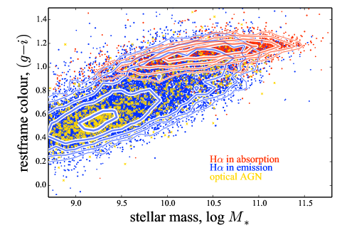
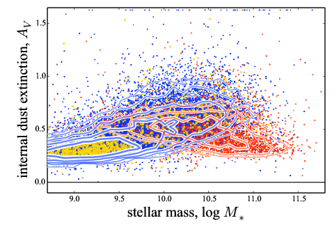
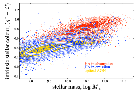
Figure 1: Stellar population parameters, as derived from SPS modelling of broadband SEDs.— The upper and lower panels show the distribution of $z<0.12$ galaxies in the colour–stellar mass plane using restframe $(g-i)$ colour, and using the intrinsic (i.e., corrected for internal dust extinction) stellar colour $(g^{*}\!-i^{*})$, respectively. The middle panel shows the dust extinction, $A_{V}$, as a function of mass, and can be thought of as linking the other two. Within each panel, the blue and red points distinguish galaxies that do or do not show clear H$\alpha$ line emission; optically identified AGN are highlighted yellow. These spectral classifications are entirely independent of the SED-fit results. Note that the AGN seem to be almost exclusively associated with the blue sequence in the $(g^{*}\!-i^{*})$ CMD. As expected, there is a strong correspondence between galaxies with old, red stellar populations, galaxies with little to no dust, and galaxies with little or no H$\alpha$ emission. That is, there is good consistency between the wholly independent photometric and spectroscopic classifications of blue/red, young/old, and active/passive galaxies. (But this does not imply that all ‘blue’ galaxies are star-forming, or vice versa.) This should give some confidence in the SPS-derived modelling used to derive all of $M_{*}$, $(g-i)$, $A_{V}$, and $(g^{*}\!-i^{*})$.

2.3.2 Effective restframe and intrinsic stellar colours

Restframe luminosities and colours are derived for each galaxy in the course of the SPS fitting process, in the same way as for $M_{*}$ or $M_{*}/L_{i}$. Naturally, these values reflect the galaxies’ constituent stellar population, modulated by interstellar dust within each galaxy. In order to more directly trace the stellar populations, we will therefore also consider dust corrected or intrinsic stellar colours. To our knowledge, this approach was first pursued by Cowie & Barger (2008). It has also been described by, e.g., Brammer et al. (2009) and Cardamone et al. (2010), on the basis of 32-band photometric redshifts from the MUSYC Narrow-Medium Band Survey (NMBS). Here, we demonstrate the feasibility and applicability of this kind of analysis for broadband SEDs, given spectroscopic redshifts.

We will focus on the intrinsic stellar $(g-i)$ colour, which we will represent as $(g^{*}\!-i^{*})$. This parameter is a very good proxy for luminosity weighted mean stellar age, $\left<t_{*}\right>$. Quantitatively, at fixed $(g^{*}\!-i^{*})$, the range in $\left<t_{*}\right>$s is everywhere $\lesssim 0.1$ dex, and $\lesssim 0.05$ dex for $(g^{*}\!-i^{*})\gtrsim 0.5$.

The values of $(g^{*}\!-i^{*})$ have also been derived in the course of the SPS fits, but can be derived to within $\lesssim 0.01$ mag from the values of $(g-i)$ and $A_{V}$ directly:

$$(g^{*}\!-i^{*})\cong(g-i)-6.0~{}A_{V}~{}.$$ (2)

The coefficient of 6.0 in this relation reflects Calzetti et al. (2000) dust extinction applied to the average (SED-fit) galaxy spectrum within our sample. The first order effect of adopting a different dust obscuration law would be a scaling of this coefficient. The choice of dust obscuration law is thus a potential source of unaccounted-for random and systematic error in our characterisations of the $(g^{*}\!-i^{*})$ CMRs (but much less so for the MFs).

The formal uncertainties in the derived values of $A_{V}$ ranges from $\approx 0.15$ mag for very blue galaxies to $\approx 0.3$ for very red ones. Again, formally, the dominant factor in these uncertainties is the imposed 0.05 mag error floor on each point in the SED (rather than the catalogued photometric uncertainties), and thus they are not strongly magnitude dependent. Given that the parameter $A_{V}$ is bounded—the amount of dust cannot be negative—these random uncertainties will lead to a systematic overestimate of $A_{V}$ in the case that the true value of $A_{V}$ is close to zero. This may in turn induce a differential systematic bias in the inferred $(g^{*}\!-i^{*})$ colours of galaxies with little to no dust (compared to those with some dust), such that the value of $(g^{*}\!-i^{*})$ may be too blue by $\sim 0.1$ mag, but not more than 0.2 mag. This limits our ability to accurately determine the locus of the CMR for red sequence galaxies, at least where such galaxies have little to no dust. Without diminishing this point, what is more important for our analysis—and especially when it comes to determining the MFs for the red and blue populations—is that we are able to make the qualitative distinction between an old stellar population and a younger one with some dust.

With this in mind, Fig. 1 shows a simple sanity check on these values. In this Figure, we distinguish between galaxies with and without strong H$\alpha$ line emission. Specifically, those galaxies with an equivalent width of 1 Å or greater are plotted as blue; AGN-host galaxies (see §2.4) are plotted as yellow crosses; the remainder of the population with H$\alpha$ seen in absorption are plotted as red.

The top panel of Fig. 1 shows the effective, restframe $(g-i)$ CMD for our $z<0.12$ sample. As expected, galaxies with H$\alpha$ seen in absorption can be seen to form a tight red sequence in $(g-i)$ colours. However, there are also many galaxies with strong H$\alpha$ emission that lie embedded in or very near to this red sequence. In general terms, these are the dusty star-formers.

The central panel of Fig. 1 shows the SED-fit values of $A_{V}$ as a function of $\log M_{*}$, using the same plotting scheme to distinguish ‘active star-formers’ from ‘quiescent’ galaxies. The emission- and absorption-line galaxies can be seen to follow different $\log M_{*}$–$A_{V}$ relations: in general, the galaxies without H$\alpha$ emission have low (but non-zero; $A_{V}\sim 0.2$–0.35) dust extinctions. While this is as expected, it is crucial to realise that the spectral classifications are independent of the SED-fit values for $\log M_{*}$ and $A_{V}$. These results thus demonstrate that our SPS fits are indeed able to reliably distinguish between old SPs with little or no dust, and dusty star-forming galaxies. (See also the discussions based on optical–NIR colours or stellar spectral diagnostics described in §9.2, below.)

For the galaxies with H$\alpha$ emission, there is a trend towards higher values of $A_{V}$ with increasing $M_{*}$. The obvious implication is that the star-forming population will be observed to become redder in $(g-i)$ towards higher $M_{*}$ by virtue of their higher dust content, independently of any variation in their stellar populations. This complicates any attempt to disentangle the young/star forming and old/passive populations based on $(g-i)$ alone.

As can be seen in the lower panel of Fig. 1, however, the active and quiescent populations are much better separated using the dust-corrected, intrinsic stellar colour, $(g^{*}\!-i^{*})$. Again, we stress that the determination of $(g^{*}\!-i^{*})$ is independent of the spectral classification—the fact that galaxies that show H$\alpha$ in absorption are almost all red in $(g^{*}\!-i^{*})$ thus demonstrates that we are in fact able to distinguish between ‘red and dead’ galaxies from dusty star-forming galaxies on the basis of their broad-band SEDs. (See §9.2.1 for further discussion of this point.)

Note that our immediate goal in this paper is not to distinguish between galaxies based on their instantaneous SFRs. (We will do this in another paper, using the H$\alpha$ measurements.) Here, our goal is to characterise galaxies’ stellar populations, using the intrinsic stellar colour, $(g^{*}\!-i^{*})$, which is a close proxy for luminosity weighted mean stellar age, $\left<t_{*}\right>$. This relies on our ability to meaningfully constrain the dust obscuration, which is what Fig. 1 is intended to show. Taken together, the three panels of Fig. 1 should thus give some confidence in the reliability of our estimates of all of $M_{*}$, $(g-i)$, $A_{V}$, and $(g^{*}\!-i^{*})$.

2.3.3 Covariant errors in $M_{*}$, $(g-i)$, and $(g^{*}\!-i^{*})$

When we come to fitting the galaxy distributions in colour–mass space in §5, we will want to account for the fact that the measurement errors/uncertainties in $M_{*}$ and $(g-i)$ are correlated. The strength of this correlation is characterised by the (Pearson) correlation coefficient,

$$\rho_{xy}\equiv\left<\frac{\left(x-\left<x\right>\right)\left(y-\left<y\right>\right)}{\sigma_{x}~{}\sigma_{y}}\right>~{}.$$ (3)

Here, $x$ and $y$ can be taken to be $\log M_{*}$ and either $(g-i)$ or $(g^{*}\!-i^{*})$; $\sigma_{x}$ and $\sigma_{y}$ are the uncertainties in these values; and $\left<Q\right>$ represents the expectation value for a generic quantity $Q$. In the parlance of Taylor et al. (2011), $\left<Q\right>$ is the Bayesian ‘most likely’ value, which is computed as the probability-weighted integral over the posterior distribution function (PDF) for that quantity (see Eq. 5 of Taylor et al., 2011). By definition, the value of $\rho$ is constrained to be $-1\leq 0\leq 1$, with the cases $\rho=-1,~{}0,~{}1$ corresponding to total anti-correlation, total independence, and total correlation, respectively. The values of $\rho_{xy}$ have been computed with the formal uncertainties $\sigma_{x}$ and $\sigma_{y}$ on a per galaxy basis in the course of the SPS fitting process. For the galaxies in our sample, the covariance between $\log M_{*}$ and $(g-i)$ is typically $\sim 0.4$; the $\log M_{*}$–$(g^{*}\!-i^{*})$ covariance is typically in the range $0.1\lesssim\rho\lesssim 0.9$.

With this definition, the error/uncertainty ellipse for any individual galaxy can then be expressed in the usual way for a bivariate Gaussian distribution:

$$p(\underline{x}{}_{i}-\underline{x})=\frac{1}{2\pi\,|\underline{\underline{\mathrm{S}}}{}_{i}|^{1/2}}~{}\exp\left[\frac{-1}{2}(\underline{x}{}_{i}-\underline{x})^{T}\underline{\underline{\mathrm{S}}}{}_{i}^{-1}(\underline{x}{}_{i}-\underline{x})\right],$$ (4)

where the vector $\underline{x}{}_{i}=(x_{i},y_{i})$ represents the observed data point and the associated error/uncertainty matrix, $\underline{\underline{\mathrm{S}}}{}_{i}$, is:

$$\underline{\underline{\mathrm{S}}}{}_{i}\equiv\left(\begin{matrix}\sigma_{x,i}^{2}&\rho_{xy,i}~{}\sigma_{x,i}~{}\sigma_{y,i}\\ \rho_{xy,i}~{}\sigma_{x,i}~{}\sigma_{y,i}&\sigma_{y,i}^{2}\end{matrix}\right)~{}.$$ (5)

Note that if $\rho_{xy,i}=0$, then the matrix $\underline{\underline{\mathrm{S}}}{}_{i}^{-1}$ is diagonal with entries $\sigma_{x,i}^{-2}$ and $\sigma_{y,i}^{-2}$, and Eq. (4) reduces to the familiar form for a 2D Gaussian with $p(x,~{}y)\propto\exp[-\frac{1}{2}(x^{2}/\sigma_{x}^{2}+y^{2}/\sigma_{y}^{2})]$.

As mentioned at the beginning of this Section, the SPS fits to the SEDs includes an error floor of 0.05 mag, and it is this decision that largely determines the formal uncertainties in $(g^{*}\!-i^{*})$. The median formal uncertainty in $(g^{*}\!-i^{*})$ within our sample is 0.18 mag; 99 % of our sample have uncertainties greater than 0.10 mag. By comparison, the observed width of the blue and red sequences in the $(g^{*}\!-i^{*})$ CMD are on the order of 0.10 mag (see Fig. 7, below); i.e., significantly smaller than the formal uncertainties.

This indicates that the formal (random) errors in $(g^{*}\!-i^{*})$ are badly overestimated. For this reason, when we model the CMD, we rescale the formal error estimates using a multiplicative factor $A_{y}$. The value of this scaling factor is fit for as a nuisance parameter along with the rest of the model. From our modelling of $(g^{*}\!-i^{*})$ CMD, we find $A_{y}\approx 0.24$; in effect, we are ultimately using nearly uniform uncertainties in $(g^{*}\!-i^{*})$ of $\approx$ 0.05 mag. Note that we do not rescale the formal uncertainties for $\log M_{*}$, nor do we adjust the correlation coefficients $\rho_{xy}$. For comparison, fitting to the $(g-i)$ CMD, the inferred value is $A_{y}\approx 1$; i.e., we see no signs that the formal uncertainties on $(g-i)$ ought to be rescaled.

2.4 Sample Definition

Our analysis is based on a subset of the full GAMA database. Specifically, we limit our analysis to those GAMA galaxies with $\log M_{*}>8.7$ (i.e., $M_{*}\gtrsim 5\times 10^{8}$ M_⊙) and $z<0.12$. These mass and redshift limits are motivated and justified in §3, below. To ensure the reliability and robustness of the spectroscopic redshift measurements, we will only consider those galaxies with nQ $\geq 3$. We only consider the $r$-band selected sample; that is, we ignore 12 H-ATLAS selected galaxies, and 355 filler targets with $19.80<r_{\mathrm{petro}}<19.85$. With these selections, we have a sample of 26368 galaxies.

98.5 % of our sample has effective surface brightness $\mu_{\mathrm{eff}}<23$. Based on the completeness curves shown in Loveday et al. (2012), we expect there to be no significant surface brightness selection effects inherited from the (SDSS) photometric parent catalogues, at least for $\log M_{*}\gtrsim 9$. We have explored the impact of surface brightness-dependent redshift failure rates, by applying completeness corrections as a function of the SDSS $r_{\mathtt{fiber}}$ magnitude. The effect on the MFs is negligible: only 1 % for $\log M_{*}=9.5$, and still just 3 % for $\log M_{*}=8.7$.

We do not explicitly exclude AGN from our analysis. In Fig. 1, we highlight the 1522 galaxies that are identified as AGN hosts, based on their position in the BPT (Baldwin, Phillips & Terlevich, 1981) diagram, coupled with an H$\alpha$ equivalent width $>$ 6 Å selection. This is similar in spirit to the WHaN selection described by Cid Fernandez et al. (2012), and was chosen to approximately reproduce the by-eye spectral classifications by Robotham et al. (2013). We note that the vast majority of these AGN hosts are inferred to have ‘normal’ B-type $(g^{*}\!-i^{*})$ colours. We have verified that none of our main results or conclusions (including the shape of the B and R MFs) change if we choose to exclude these galaxies.

3 Quantifying and accounting for incompleteness as a function of mass, colour, and redshift

The upper panels of Fig. 1 show the basic data for our analysis; namely the $(g-i)$ and $(g^{*}\!-i^{*})$ CMDs. In both cases, the relative number of red sequence galaxies in both the $(g-i)$– and the $(g^{*}\!-i^{*})$–$M_{*}$ diagrams peaks somewhere around $\log M_{*}\sim 10.5$. There is a drop-off in the fraction of red galaxies below this mass, such that there is little to no clear evidence for a continuation of the $(g^{*}\!-i^{*})$ red sequence below $\log M_{*}\sim 9.5$. The principal difficulty in interpreting this result is the extent to which our $z<0.12$ sample is sensitive to truly ‘red and dead’ galaxies at these relatively low masses of $\log M_{*}\lesssim 10$. We explore this issue in two complementary ways in this Section.

3.1 Incompleteness and $\mathbf{1/V_{\mathrm{max}}}$ corrections

We use the standard $1/V_{\mathrm{max}}$ technique (Schmidt, 1968) to account and correct for incompleteness as a function of both stellar mass and stellar population. The essential idea behind $1/V_{\mathrm{max}}$ corrections is to estimate that maximal volume, $V_{\mathrm{max}}$, over which any given galaxy would satisfy our ($r$-band) selection criteria. If we can estimate or predict the apparent $r$-band magnitude for a given galaxy if it were to be placed at some generic redshift $z^{\prime}$ as $r(z^{\prime})$, then $V_{\mathrm{max}}$ can be derived by integrating over the survey volume in which $r(z^{\prime})$ is brighter than our selection limits. This has been done in the course of the SPS SED fits, using the single best-fit SPL template, as described in Taylor et al. (2011).

There are two things that need to be accounted for when estimating the values of $V_{\mathrm{max}}$ for galaxies in our sample. First, there is the fact that the GAMA target selection has been done on the basis of SDSS petro magnitudes. We can account for this by calculating $r(z^{\prime})$ as $r_{\mathrm{petro}}+\Delta r(z^{\prime})$, where $r_{\mathrm{petro}}$ is the (foreground extinction corrected) SDSS petro magnitude, and $\Delta r(z^{\prime})$ can be thought of as the $z^{\prime}$-dependent $k$-correction implied by the SPS fit. Second, there is the difference between the cosmological redshift, which maps directly to comoving distance, $D$, as $cz\approx H_{0}D$, and the heliocentric redshift, which includes Doppler shifting from peculiar motions due to local bulk flows. This is done by recognising that $(1+z^{\prime}_{\mathrm{helio}})=(1+z^{\prime})(1+v_{\mathrm{flow}}/c)$, where $v_{\mathrm{flow}}$ is the peculiar velocity arising from local bulk flows (see §2.1). The value of $V_{\mathrm{max}}$ is then defined via the maximum (flow-corrected) redshift, $z^{\prime}$, for which both the $r(z^{\prime})<19.8$ and $z^{\prime}<0.12$ selection criteria are satisfied.

We have experimented with using a density corrected $1/V_{\mathrm{max}}$ weighting to account for large scale structure at the lowest redshifts. Baldry et al. (2012) have shown first that large scale structure in the $z<0.06$ GAMA volume can have a significant impact on the recovered mass functions, and second that these effects can be largely mitigated by using a Density Defining Population. Our case is rather different, however: even for $\log M_{*}\sim 9$, most of our galaxies lie at $z>0.06$. (Plus, the GAMA-II survey area is 25 % larger, as well as 0.4 mag deeper in two of three fields.) Using the Baldry et al. (2012) scheme, the corrections to the MFs are at the level of $\sim 5$ % for $\log M_{*}\lesssim 9.5$. The problem is that using different DDPs yield different corrections. The difference in the recovered $\log M_{*}\lesssim 9.5$ MF when defining the DDP to be $\log M_{*}>10.5$ or $\log M_{*}>11$ galaxies is on the order of $\sim 3$ %; that is, comparable to the size of the corrections themselves. For this reason, we do not apply these negligible corrections.

Note that to protect against catastrophic errors in the $V_{\mathrm{max}}$ estimates, we limit the maximum relative weighting of any individual galaxy to be $V_{\mathrm{survey}}/V_{\mathrm{max}}<30$. In effect this means that we will be under-correcting for any galaxies that have $z_{\mathrm{max}}<0.038$. As can be seen in Fig. 2, this decision affects only 16 galaxies in our $\log M_{*}>8.7$ sample. Limiting our sample to being $z>0.035$ excludes all of these ‘problem’ objects. With this $z>0.035$ limit, the inferred mass functions are depressed by $\lesssim 0.1$ dex for $\log M_{*}\lesssim 9$ (due to incompleteness), but none of our qualitative results or conclusions change.

We have done the usual consistency tests (Schmidt, 1968) to check the reasonableness of these incompleteness corrections. We have verified that where the values of $V_{\mathrm{max}}$ imply that we are properly volume limited (i.e., mass complete), the median $z$ is approximately equal to the volumetric centre of the $z<0.12$ survey window. For the bluest galaxies ($0.25<(g-i)<0.50$), this is true for $\log M_{*}\gtrsim 9.5$; for the reddest galaxies, this is true for $\log M_{*}\gtrsim 10$. We have also verified that the median value of $V(z)/V_{\mathrm{max}}\approx 1/2$; even after binning by colour, this is true for all masses $\log M_{*}\gtrsim 8.7$.

The problem is that there are too few low mass red galaxies in our sample for us to look at our completeness for $(g-i)\gtrsim 1$ galaxies with $\log M_{*}\lesssim 9$ in this way. We have only 12 galaxies with $(g-i)>1.0$ and $\log M_{*}<9$ in our sample, all of which are at $z\lesssim 0.04$. Leaving aside the question of field-to-field variance, the concern is whether the apparent dearth of such red, low-mass galaxies in the GAMA catalogues is a fair characterisation of the GAMA $z\lesssim 0.04$ survey volume, or if instead we have over-estimated our sensitivity to these very faint galaxies.

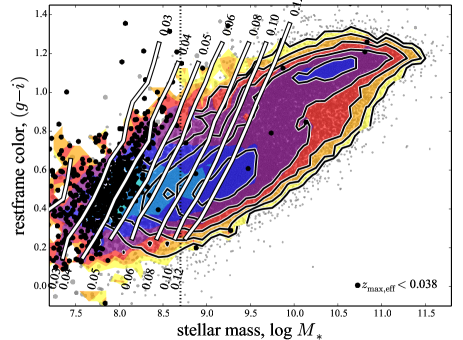
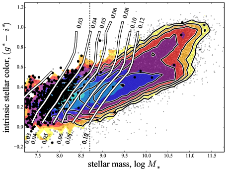
Figure 2: Completeness limits as a function of mass and colour.— This figure is discussed at length in §3. The upper and lower panels of this Figure show the $(g-i)$ and $(g^{*}\!-i^{*})$ CMDs, respectively, for all $z<0.12$ galaxies in the GAMA catalogue. In both panels, the points show individual galaxies, with the sizes of each point chosen to reflect the implied $1/V_{\mathrm{max}}$ incompleteness corrections (see §3.1). The line contours show the observed data density without corrections for incompleteness; the filled coloured contours show the $1/V_{\mathrm{max}}$-weighted results. The white lines show empirical estimates of how the $r_{\mathrm{petro}}<19.8$ selection limit maps onto the CMD at different redshifts (see §3.2). The $z\approx 0.12$ curve shows that we are complete (volume limited) for all galaxy colours for $\log M_{*}\gtrsim 10$. Our decision to limit our $V_{\mathrm{survey}}/V_{\mathrm{max}}$ weightings to $\leq 30$ effectively means that we will be under-correcting for incompleteness for $z<0.038$; those galaxies with relative weightings $>30$, or $z_{\mathrm{max}}<0.038$, are plotted in black. The extent to which the empirical completeness curve for $z\approx 0.04$ approximately bounds the black $V_{\mathrm{survey}}/V_{\mathrm{max}}>30$ points thus shows the consistency between these two complementary means of estimating our selection limits as a function of colour, mass, and redshift. Our analysis is thus conservatively limited to $\log M_{*}>8.7$ (i.e., $M_{*}\gtrsim 5\times 10^{8}$ M_⊙); this limit is shown as the vertical dotted line.

3.2 An empirical characterisation of our completeness limits as a function of mass, colour, and redshift

In Fig. 2, we again show the distribution of $z<0.12$ galaxies in the $(g-i)$ and $(g^{*}\!-i^{*})$ colour–mass diagrams. In both panels, the filled, coloured contours show the inferred bivariate colour–mass distribution function after applying our $1/V_{\mathrm{max}}$ weightings to account for incompleteness. These contours should be compared to the black and white line-contours, which show the raw, observed data-density in the colour–mass diagrams; i.e., without incompleteness corrections.

We have plotted the individual galaxies in our sample as the gray points; the size of each point directly reflects the magnitude of the $1/V_{\mathrm{max}}$ factor used to account for incompleteness. The black points in these panels highlight those few galaxies with relative weightings $w=V_{\mathrm{survey}}/V_{\mathrm{max}}>30$. Since we have chosen to limit our weightings to be $\leq 30$, these are the galaxies for which (formally) we would be under-correcting for incompleteness. It is entirely possible, however, that these points reflect somehow catastrophic errors in our $V_{\mathrm{max}}$ and/or $M_{*}$ estimations: there are many more galaxies with similar masses and colours for which the implied values of $w$ are considerably smaller.

In order to investigate our sensitivity to low mass, red sequence galaxies further, we have therefore sought to quantify our sample completeness limits in a way that is independent of our $V_{\mathrm{max}}$ calculations. We have done so by taking all observed galaxies and simply scaling their total luminosities/masses down to match the $r_{\mathrm{petro}}=19.8$ selection limit. Then, by dividing our sample in narrow redshift intervals of width $\Delta z=0.01$ and centred on $z=0.01$, 0.02, …, 0.12, we take the median value of this limiting mass in narrow bins of restframe or intrinsic colour.

This analysis thus provides an empirical description of our 50 % mass completeness limits, as a function of redshift and colour, but in a way that is independent of the SPS fits that have been used to derive $M_{*}$, $(g-i)$, and $(g^{*}\!-i^{*})$; the results are shown as the heavy white-and-black lines in Fig. 2. The $z=0.03$, 0.04, 0.06, 0.08, and 0.10 curves can be taken as corresponding to relative volume completenesses of $V_{\mathrm{max}}/V_{\mathrm{survey}}\approx$ 0.02, 0.04, 0.13, 0.30, and 0.59, respectively.

The first point to make is that this independent, empirical characterisation of our mass-completeness limits agrees very well with the results of our $1/V_{\mathrm{max}}$ calculations. The fact that the distribution of the black points in each panel of Fig. 2 is approximately bounded by the empirical completeness limit for $z=0.04$ should thus give some confidence in our $V_{\mathrm{max}}$ estimates. In the same way, the $z=0.12$ curve can be taken as indicative of where we are truly volume limited. Taken together, these two curves thus bound the region of the colour-mass diagrams in which our incompleteness corrections are important and reasonable. Since the black and colour-filled contours in these panels show the data density without and with $1/V_{\mathrm{max}}$ corrections, where these contours coincide shows where incompleteness corrections are unnecessary. Again, the fact that the $z=0.12$ curve very accurately bounds the regions in both the $(g-i)$–$M_{*}$ and $(g^{*}\!-i^{*})$–$M_{*}$ diagrams over which this is true should give confidence in our $V_{\mathrm{max}}$ estimates.

3.3 Are we seeing the low mass end of the red population?

Given all of the above, are we (or are we even capable of) seeing the low-mass end of the red sequence? We can be all but certain that there are very few red galaxies with $8.7<\log M_{*}<9.0$ galaxies in the $z<0.06$ GAMA survey volume ($\approx 3\times 10^{-3}$ Gpc³). Addressing this question any further is made problematic, however, by the effects of large scale structure, and particularly by the degree to which low-mass and red galaxies are biased towards rich-group and cluster environments.

Geha et al. (2012) have looked at the fraction of low mass galaxies in SDSS that are (spectroscopically) identified as having both old stellar populations and no ongoing star formation, and found that all such galaxies with $\log M_{*}\sim 7$–9 are satellites within 1.5 Mpc (comoving, projected) of a $\log M_{*}\gtrsim 10.4$ ‘host’ galaxy. For our sample, the number density of $\log M_{*}>10.4$ galaxies at $z<0.06$ is actually 10 % higher than for $0.06<z<0.12$: that is, we may in fact be biased towards old, low mass galaxies. Based on the group catalogue described by Robotham et al. (2011), our sample contains 580 $\log M_{*}>10.4$ and $z<0.06$ galaxies, in 232 separate groups, 22 of which have multiplicities of 10 or more. Included in these groups are 194/2895 (6.7 %) of the $\log M_{*}<9$ and $z<0.06$ galaxies in our sample, all of which are within 0.5 Mpc (cf. the Geha et al. (2012) limit of 1.5 Gpc) of their hosts. These numbers give some sense of the environments we are probing—i.e., from isolation up to low- and-moderate sized groups.

At the same time, we point out that based on the derived values of $V_{\mathrm{max}}$, the results shown in Fig. 2 suggest that our completeness may still be $\gtrsim 95$ % even for $\log M_{*}\sim 8.5$. Further, we stress that our relative volume completeness is greater than 50 % ($z_{\mathrm{max,eff}}\gtrsim 0.095$) for even the reddest galaxies with $\log M_{*}>9.5$; we consider it highly unlikely that our results above this mass scale are strongly affected by incompleteness. We have also verified that none of our results change significantly if we limit our analysis to $z<0.06$, or to $\log M_{*}>9.5$.

In light of all this, and with the above caveats, we continue our analysis with a nominal mass limit of $\log M_{*}>8.7$.

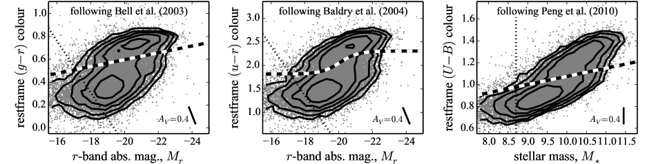
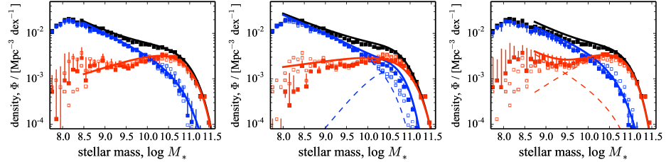
Figure 3: Reproducing previous analyses using our GAMA sample, and illustrating the crucial importance of how the terms ‘red’ and ‘blue’ are defined.— The upper panels show the selection used to separate red from blue galaxies by Bell et al. (2003), Baldry et al. (2004), and Peng et al. (2010), in either a colour-magnitude or colour-mass diagram. In these panels, the points show all $z<0.12$ galaxies from GAMA, and the contours show the (logarithmic) data density, without corrections for incompleteness. The lighter dotted line shows our sample selection limit of $\log M_{*}=8.7$, and the heavy black-and-white lines show the binary red/blue cuts used or advocated by each set of authors. In the lower panels, we show the inferred mass functions for red and blue galaxies when applying these different authors’ cuts. In these panels, the smooth curves show these authors’ fits, which have all been derived using SDSS data. Where these fits are the sum of two Schechter functions, the separate components are shown as the thin dashed lines. These should be compared to the points, which show what we find when we apply each of these red/blue selections to our GAMA sample. We are able to reproduce each set of results with our data. However, the different authors’ fits should also be compared to one another. To help with this, in each of these panels, the results from the other two analyses are reproduced as the smaller, open squares. There are major qualitative and quantitative differences between the results of the different analyses, which are entirely due to the different ways of defining ‘red’ and ‘blue’.

4 What — if anything — do you mean by ‘red’?

4.1 The state of play

There are a number of ways of discriminating between ‘developed’ and ‘developing’ galaxies, based on, e.g., restframe colour, spectral classification, Hubble type (i.e., morphology), or Sérsic index (i.e., structure). There is considerable, but by no means total, overlap between these different kinds of selections (see, e.g., Robotham et al., 2013). However, as we will show in future papers in this series, inappropriate conflation of the terms red/blue, early-/late-type, and quiescent/active has the potential to be dangerously misleading.

Our overarching goal in this work is to look at the bimodality as seen in the optical CMD—in other words, we are specifically interested in the bimodality that exists in galaxies’ stellar populations. With this in mind, our specific goal is to derive a quantitative description of phenomenology of the joint colour–mass distribution of galaxies, in terms of both the CMRs and the MFs for the apparently distinct ‘red’ and ‘blue’ populations.

As a motivating introduction to our method for attacking this problem, consider Fig. 3. In this figure, we show our best attempts at reproducing the SDSS-based analyses of Bell et al. (2003), Baldry et al. (2004), and Peng et al. (2010) using our $\log M_{*}>8.7$ and $z<0.12$ GAMA sample. In the upper panels of this Figure, we show the different ways that each set of authors have separated the red and blue galaxy populations, based on either a colour-magnitude, or a colour–mass diagram. In rough terms, the Bell et al. (2003) cut can be seen as a relatively conservative means of selecting ‘red’ galaxies: the selection line appears to hug the lower limits of the red sequence. By contrast, the Peng et al. (2010) cut is rather aggressive: it falls closer to the upper edge of the blue cloud. The cut advocated by Baldry et al. (2004) is in a sense intermediate: it can be seen to be aggressive at lower luminosities, and conservative at higher luminosities. In the lower panels, the filled squares show the inferred red/blue galaxy mass functions, when applying each of the different selections to our GAMA dataset. In general, the agreement between each set of SDSS- and GAMA-derived results is very good.

Further to our discussion of incompleteness in the previous section, we also highlight the fact that the GAMA MFs—including the red MFs—are continuous for $\log M_{*}\gtrsim 8.5$. This is despite the distracting and unfortunate downtick in the number of galaxies with $\log M_{*}\approx 8.7$ (our mass selection limit). We are not obviously incomplete for $8.7\lesssim\log M_{*}\lesssim 9$.

There are some obvious systematic differences in the inferred number densities for $\log M_{*}\lesssim 10$. As a result, the integrated number density of galaxies with $\log M_{*}>8.7$ from GAMA is 7 %, 12 %, and 13 % lower than that from Bell et al. (2003), Baldry et al. (2004), and Peng et al. (2010), respectively. (Not surprisingly, however, we agree almost exactly with Baldry et al., 2012, not shown). These differences come down to the different means of estimating stellar masses.

The role of various kinds of systematic errors/uncertainties in determining the net MF (the black curves and points in Fig. 3) has been explored by Baldry et al. (2012); that is not our main purpose here. For our purposes, it is sufficient to note that having controlled for everything we can (e.g., taking SDSS model fluxes as total; matching IMFs and cosmologies) we match the inferred integrated stellar mass density for $\log M_{*}>9.5$ to within 3–4 % in each case.

Instead, we are specifically concerned with sources of systematic error or uncertainty on the MFs for the ‘red’ or for the ‘blue’ galaxy populations. That is, we are particularly interested in the red and blue lines/points shown in Fig. 3.

In this regard, the most noticeable discrepancy is our failure to reproduce the apparent upturn in the red mass function seen by Peng et al. (2010) for $\log M_{*}\lesssim 9.5$. We suggest that at least part of this discrepancy is due to differences in how we have derived our $(U-B)$ colours. Comparing our $(U-B)$ colours, derived in the course of the SPS fits, to those from kcorrect (Blanton & Roweis, 2007), we find that there is considerable scatter (at the level of 0.15 mag), even when analysing the same SDSS petro photometry. We have tried simply perturbing our $(U-B)$ colours by 0.15 mag. This has the net effect of scattering a small fraction of ‘blue’ galaxies into the ‘red’ sample, which leads to a significant increase in the inferred numbers of red galaxies, as illustrated by the thin vertical lines in the lower-right panel of Fig. 3. Note that the other MFs are more robust to photometric scatter at this level, as is shown.

We also note that, in the middle panel, the agreement between our GAMA-derived results and the Baldry et al. (2004) fits is imperfect, particularly for the red MF. We will defer detailed discussion of this discrepancy to §9.1. For now, we simply note that the Baldry et al. (2004) cut is based on their fits to the MF, rather than the other way around; we therefore expect some small quantitative differences between the Baldry et al. (2004) fits and the MFs derived using the Baldry et al. (2004) cut. At this stage, the important point is that we see the same qualitative results.

In order to facilitate easy comparison between the results of these different analyses, in each of the lower panels of Fig. 3, there are two sets of small open squares, which re-plot the results of the other two analyses. The range spanned by these points thus reflects the systematic uncertainty on the blue and red mass functions, arising from the different ways that the ‘blue’ and ‘red’ galaxy samples have been selected/defined. Note in particular the size of these uncertainties at and around the knee of the mass function, as well as at low masses, for both the red and blue mass functions.

Based on Fig. 3, we make the following four observations:

• Comparing the different authors’ fit MFs to one another, there are important discrepancies in the shapes of both the red and the blue mass functions for $10\lesssim\log M_{*}\lesssim 11.3$. This is unfortunate, because this leads to large uncertainties ($\gtrsim 0.3$ dex) in the mass-scale at which galaxies transition from one population to the other.

• There are also large discrepancies in the values of the low-mass slope of the red mass function: it might be slowly declining ($\alpha\approx-0.7$), or nearly constant ($\alpha\approx-0.9$), or has a sharp upturn ($\alpha\approx-1.5$). This is unfortunate, as it leaves the behaviour of the low mass red population largely unconstrained.

• Further, there is not even consensus as to how the two MFs ought to be described and understood qualitatively. The Bell et al. (2003) MFs are each well described by a single Schechter function; Baldry et al. (2004) finds a need for a second Schechter component to describe the blue MF; Peng et al. (2010) find instead that it is the red MF that needs a second Schechter component.

• That we can reproduce each set of results using our dataset shows that these discrepancies come from differences in how the data are analysed, rather than differences in the data themselves.

In other words, current understanding of the MFs for the red and blue galaxy populations is limited by systematic errors. As mentioned in the Introduction, measurements of the MFs for the red and blue galaxy populations have played a pivotal role in informing our understanding of galaxy formation and evolution. It is therefore critically important to understand how and why there can be such large discrepancies between the results of these different analyses. Only then will we be able to formulate an analytical approach that will allow us to robustly measure these quantities.

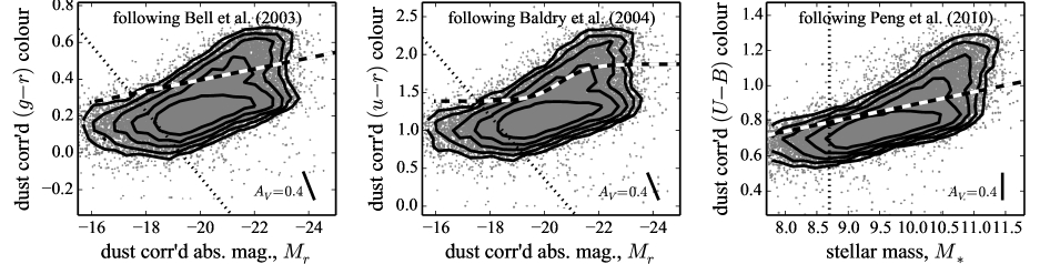
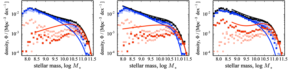
Figure 4: Adapting previous analyses to account for dust, and illustrating the critical importance of how the terms ‘red’ and ‘blue’ are defined.— In the upper panels, we have applied dust corrections to the data, to show intrinsic stellar colours and magnitudes. We have also rescaled the Bell et al. (2003), Baldry et al. (2004), and Peng et al. (2010) selection lines, so as to retain those ‘red and dead’ galaxies with low (but non-zero) dust extinction. The lower panels show the mass functions that follow from these cuts. Compared to Fig. 3, these selections lead to a very different picture of the field galaxy population. Note that we are not suggesting that the results shown in this Figure provide a fair or accurate representation of the bimodality in galaxies’ stellar populations. Instead, the conclusion to be drawn from this Figure is that the inferred MFs depend entirely on how the ‘red’ and ‘blue’ samples are selected/defined. Compared to one another, the red galaxy MFs in these figures differ by a factor of $\sim 2$; compared to the MFs in Fig. 3, the difference is a factor of $\sim 10$. Lacking any solid theoretical basis for preferring any one selection line over any other, what is needed is an objective, data-driven means of identifying and separating the ‘red’ and ‘blue’ populations.

4.2 Dust is not the (only) issue.

Given that there appears to be a better separation between the ‘red’ and ‘blue’ populations in the $(g^{*}\!-i^{*})$ CMD shown in Fig.s 1 and 2, the natural question is whether the discrepancies described in the previous section can be alleviated or removed by focusing on intrinsic stellar colours/magnitudes. What happens if we try modifying these analyses to account for dust obscuration/extinction?

We address this question in Fig. 4. The main difference between this Figure and Fig. 3 is that we have now shifted to intrinsic (i.e., dust corrected) stellar colours and luminosities, so as to more directly probe galaxies’ stellar populations.

As discussed in §2.3.2 and shown in Fig. 1, the lowest values for the SED-fit dust extinctions is $A_{V}\approx 0.2$, even for galaxies with no H$\alpha$ emission. In light of this fact, we need to also rescale each of the selection lines shown in the upper panels of Fig. 3. What we have done is to shift each selection line by the equivalent of $A_{V}=0.4$ mag. This ‘correction’ is much larger than the expected dust obscuration for a canonically ‘red and dead’ galaxy. It should be thought of as a conservative way to exclude the dustiest galaxies, while retaining those galaxies with genuinely ‘red’ stellar populations.

The bottom panels of Fig. 4 shows the MFs for ‘red’ and ‘blue’ galaxies, selected in this way; the selections themselves are shown in the upper panels. It is clear that adopting these selections would lead to a rather different picture of the makeup of the field galaxy population.

Comparing the range of values for the red MF that come from these different selections, the differences are at the level of a factor of $\sim 2$. This is considerably larger than the differences seen in Fig. 3. That is, modifying these selections to account for dust exacerbates the tension between these different authors’ results, rather than alleviating it. (This implies that, even when looking at dust-corrected, intrinsic stellar colours, there is still substantial overlap between the ‘blue’ and ‘red’ populations. We will show in Fig. 7, below, that this is indeed the case.) No less worrying is the size of discrepancy between the $\log M_{*}\lesssim 10$ MFs for the $(g^{*}\!-i^{*})$-selected ‘red’ galaxies (Fig. 4) and the $(g-i)$–selected ones (Fig. 3). Perhaps not surprisingly, the size of this discrepancy is very sensitive to how much one chooses to shift each selection line—that is, how much dust to allow for in otherwise ‘red sequence’ galaxies.

So which of the six analyses we have now trialled is right? Are the results shown in Fig. 4 any more or less reliable or meaningful than those shown in Fig. 3?

The crux of the problem is that there are no clear theoretical grounds for preferring any one of these ‘red’/‘blue’ cuts over any other. In the absence of a solid, astrophysically meaningful argument for such a cut, this is necessarily true—without further information, we have no compelling way to answer this question. While we might offer some empirical or phenomenological argument in support of our specific cut, the point is that this decision will always be arguable; that is, arbitrary. This is a point that we will return to in §7.2 and §9.2.

For now, we can say with some confidence that these different results can be taken to approximately bracket the range of allowed values for the red/blue MFs that come from reasonable choices for hard-cut red/blue selections. The truth probably lies somewhere between the different results shown in Fig. 3 and Fig. 4. This is not very satisfactory, however, as it means that the shapes of the red and blue MFs are not even well constrained qualitatively, much less quantitatively.

4.3 The nature of the distinction between ‘red’ and ‘blue’

In short: the quantitative and qualitative discrepancies between the results shown in the lower panels of Fig. 3 and Fig. 4 are entirely due to the different ways that each set of ‘red’ and ‘blue’ samples has been selected—or, said another way, to the different operational definitions of the terms ‘red’ and ‘blue’. For example, the fact that Peng et al. (2010) see an upturn to the red mass function at low masses—where Bell et al. (2003) and Baldry et al. (2004) do not, despite their using essentially similar datasets, and even pushing to lower masses—is a direct consequence of the fact that the Peng et al. (2010) selection line is relatively bluer than earlier authors.

It is therefore worth reflecting on the two implicit assumptions that underpin the use of a hard cut to separate ‘red’ from ‘blue’ galaxies, and thus the results shown in Fig. 3 and in Fig. 4. First, it is presupposed that ‘blueness’ and ‘redness’ are physically meaningful designations, inasmuch as they encapsulate some fundamental distinction between the origins or natures of two distinct kinds of galaxies. The second, and more problematic, assumption is that there is something special—something astrophysically meaningful—about the particular boundary used to separate the two galaxy classes.

The methodological appeal of such an approach is that it is well-defined, inasmuch as the hard cut can be written explicitly and exactly, which makes such analyses easily reproducible. In the early days of the SDSS, the astronomical motivation was also clear. Strateva et al. (2001), Blanton et al. (2003a), and many others had shown that there is substantial (but not total) overlap between a ‘red sequence’ sample and an ‘early type’ sample selected on the basis of Sérsic index. In this way, ‘redness’ and ‘blueness’ were thought of as indirect proxies for structure, and thus for morphology. As was common at the time, Bell et al. (2003), Baldry et al. (2004) and others presented their mass function determinations for ‘red’ and ‘blue’ galaxies in terms of the Hubble early- and late-type classifications. Peng et al. (2010), on the other hand, have phrased their results in terms of ‘star-forming’ and ‘quiescent’ galaxies. (This is also the explicit goal of, for example, some colour–colour selections, which are discussed further in §9.2.)

Here again, we caution against this conflation of terminology when interpreting these results. While ‘early type’ samples selected on the basis of colour, spectral type, morphology, and structure are often treated as if they are interchangeable, it is now becoming clear that they are not. This point, and its importance, have most recently been forcefully made by Schawinski et al. (2014), who consider the CMDs for morphologically classified ‘early-’ and ‘late-types’.

Further, the use of a hard cut overlooks the empirical fact of scatter around each of the distinct CMRs for the ‘red’ and ‘blue’ populations, however they are defined. Any number of authors have shown that, at fixed magnitude or mass, the distribution of galaxies’ (optical) colours can be well described as the sum of two Gaussians, and that the separation and widths of these two Gaussian distributions are such that there is considerable overlap between the two (see, e.g., Balogh et al., 2004; Baldry et al., 2004; Bell et al., 2004b; Williams et al., 2009; Wolf et al., 2009; Nicol et al., 2011; Coppa et al., 2011). Considering these two distributions as arising from two distinct populations, the implication is that the use of a hard red/blue cut will yield samples that are both incomplete, and contaminated (see also, e.g., Driver et al., 2006). We will return to this issue towards the end of this paper, in §9.1.

4.4 All galaxies are red, but some are redder than others.

In light of the above, we will not take quite so simple a view. We will assume that there is some meaningful astrophysical distinction to be made between the two populations: that there is some unknown astrophysical process that acts to determine whether any given galaxy is a member of either the ‘blue’ or the ‘red’ population. That is, we will assume that there are two distinct CMRs. But we will also allow that some ‘hidden’ parameter (or parameters) mean that, at fixed mass, there are a range of colours among the members of each of the two populations, to the extent that these two distinct populations are observed to overlap in the CMD. That is, we will assume that there is some intrinsic scatter around each of the two CMRs.

Adopting this (non-controversial) view of two overlapping populations, the conceptual difficulty that arises is that some members of the ‘blue’ population will have quantitatively redder $(g-i)$ or $(g^{*}\!-i^{*})$ colours than some members of the ‘red’ population. Further, two galaxies might have identical values of $M_{*}$ and $(g-i)$, but one might ‘really’ belong to the ‘blue’ population, and the other to the ‘red’ one. Without further information, it would be impossible to unambiguously determine which is which.

This means that any ‘red’/‘blue’ classification of individual galaxies can only be done probabilistically, in terms of the odds that that galaxy has been drawn from either the ‘red’ or the ‘blue’ population. While our approach brings these conceptual quandaries into sharp focus, we stress that similar criticisms can be levelled at the simple, binary ‘blue’/‘red’ distinction used above: the inferred scatter around the CMRs derived for the hard-cut ‘blue’ and ‘red’ populations leads to precisely the same conundrum.

Without solid astrophysical justification, the terms ‘blue’ and ‘red’ must be understood to be defined operationally, and as such are useful only as qualitative descriptors. In acknowledgement of this point, we will from now on abandon the terms ‘blue’ and ‘red’ as classifiers, and instead use the more generic idea of a B- and an R-population. Note that these descriptors do not properly apply to individual galaxies, but instead to distinct populations of galaxies.

Obviously, the designations B and R have been chosen with a nod towards one being for the bluer population, and the other for the redder one. But we want to be absolutely clear that these designations are based on phenomenological descriptions of the joint colour-magnitude distributions and should not be taken to be rigorously grounded in astrophysical theory. Any astrophysical interpretation of our descriptive B- and R- population modelling, including those offered in §8, must be done with care.

Let us stress in particular that we are not explicitly trying to select galaxies that are quiescent, quenched, early-type, etc. Our explicit goal here is only to distinguish between the generic ‘developed’ and the ‘developing’ galaxy populations on the basis of their stellar populations. In this sense, all that the B and R designations are intended to encapsulate are the distributions of luminosity weighted mean stellar ages, as probed by either $(g-i)$ or $(g^{*}\!-i^{*})$.

Of course, at least for moderate- to high-masses ($\log M_{*}\gtrsim 9.7$), it turns out that the galaxies that comprise the R population largely conform to the prevalent notion of ‘red and dead’ or ‘quenched’ (see §9.2, as well as Fig. 1). This being the case, our results can be used to gain insight on the process of quenching, but only insofar as our operational definition of ‘red’- or ‘R’-ness can be taken to mean ‘quenched’.

While our approach brings this issue into sharp focus, the same degree of caution is merited when interpreting the results of past studies of ‘blue’ and ‘red’ galaxies: bearing in mind the qualitative and quantitative discrepancies between the results shown in Fig. 3 or Fig. 4, which of the selections shown in these figures can be said to best represent the idea of ‘quenched’?

Adopting the working hypothesis of two distinct but overlapping B- and R-populations in the CMD, the question becomes technical: how best to distinguish and characterise the two populations on the basis of the observed CMD. While the designations ‘B’ and ‘R’ must be understood to be qualitative, inasmuch as they are phenomenological, we want to be able to classify galaxies quantitatively. This can be done probabilistically, according to the chances that they are members of either the B or R population. Further, we want these classifications to be objective. In order to achieve these goals, it is necessary to describe or otherwise account for the actual underlying colour distributions, including the degree of overlap, and as a function of mass. This is therefore the task that we have undertaken.

5 Method — Objectively Classifying Galaxies in the Colour–Mass Diagram

This section is devoted to describing and validating our descriptive modelling of the bivariate or joint $(g-i)$ and $(g^{*}\!-i^{*})$ colour–mass distributions for field galaxies at $z<0.12$. The most general form of our model is laid out in §5.1, including definitions and descriptions of the 40 parameters that define the model in its most general form. In §5.2, we describe the numerical methods that have been used to fit for the free parameters. In §5.3, we describe the process by which we have selected the best and simplest description of the data from within the more general family of models that we have considered. (For the more motivated reader, we present a pedagogical development of the model in Appendix A, in which we build up our formalism as successive generalisations of the conventional weighted-$\chi^{2}$ approach to fitting a single line.)

The conceptual basis of our descriptive modelling is this: that the observed data are a sampling of some ‘true’, astrophysical, bivariate colour–mass distribution. This being the case, our data can be seen to have been drawn from—generated by—some 2D probability distribution function, $p(\underline{x}^{\prime})$, where $\underline{x}^{\prime}=(x^{\prime},\,y^{\prime})$ denotes some generic location in our 2D data plane. (In this section, we will thus use $x$ and $y$ to further abbreviate the quantities $\log M_{*}$ and either $(g-i)$ or $(g^{*}\!-i^{*})$.)

We cannot absolutely know the ‘true’ form of the distribution function $p(\underline{x}^{\prime})$. So instead, we aim to construct a parametric description for what $p(\underline{x}^{\prime})$ might be, and use the data to constrain the possible and even likely form of $p(\underline{x}^{\prime})$. Let us denote the full set of parameters used or required to describe $p(\underline{x}^{\prime})$ as $\mathbf{P}$.

Assume for a moment that we know or can guess the correct form of $p(\underline{x}^{\prime}|\mathbf{P})$. Naturally, one does not observe this distribution directly. Instead, observational errors mean that the observed distribution in the $(x^{\prime},\,y^{\prime})$ plane will be a smeared out version of the true distribution. Let us also assume that that the observational errors/uncertainties for a given data point, $\underline{x}{}_{i}=(x{}_{i},\,y{}_{i})$, are Gaussian, and so can be described by the covariance matrix $\underline{\underline{\mathrm{S}}}{}_{i}$ (see Equations 3—5). Using $\mathcal{G}_{2}(\underline{x}{}_{i},\underline{\underline{\mathrm{S}}}{}_{i})$ as shorthand for a bivariate Gaussian, the likelihood of observing a particular datum $i$ is then given by the convolution of the ‘true’, underlying distribution and the bivariate Gaussian that describes that measurement, and its associated uncertainty; i.e.,

$$\begin{split}\mathcal{L}{}_{i}(\underline{x}{}_{i},\underline{\underline{\mathrm{S}}}{}_{i}|\mathbf{P})&=\int\mathrm{d}\underline{x}^{\prime}~{}p(\underline{x}^{\prime}|\mathbf{P})~{}\mathcal{G}_{2}(\underline{x}{}_{i}-\underline{x}^{\prime},\underline{\underline{\mathrm{S}}}{}_{i})\\ &=p(\underline{x}^{\prime}|\mathbf{P})\otimes\mathcal{G}_{2}(\underline{x}{}_{i},\underline{\underline{\mathrm{S}}}{}_{i})~{};\end{split}$$ (6)

Note that to satisfy the requirement that a point actually be observed, we impose to the normalisation conditions that the integral over ($x,y$) space for $p$ and $\mathcal{G}_{2}$, and hence $\mathcal{L}{}_{i}$, be equal to one.

It is crucial to recognise that the value of $p$, and thus the value of $\mathcal{L}{}_{i}$, can only be computed—indeed, are only defined—given an assumed or trial set of values for each and every of the parameters in $\mathbf{P}$. In recognition of this fact, these quantities have been written in Eq. (6) and all that follows as $\mathcal{L}{}_{i}(\underline{x}{}_{i},\underline{\underline{\mathrm{S}}}{}_{i}|\mathbf{P})$ and $p(\underline{x}{}_{i}|\mathbf{P})$.

The crux of the problem is then to construct an appropriate parametric description of $p(\underline{x}^{\prime}|\mathbf{P})$. That is our task in this section. At this stage, the casual or credulous reader whose interest lies only in our results may wish to skip these technical sections, and move directly to §6, in which we demonstrate the quality of our fits to the observed bivariate $(g-i)$– and $(g^{*}\!-i^{*})$–$M_{*}$ distributions.

5.1 A descriptive model for the distribution of observed data points in the CMD

In order to accommodate the apparent bimodality in the $(g-i)$ and $(g^{*}\!-i^{*})$ CMDs, we split the model for the ‘true’, astrophysical bivariate colour–mass distribution—i.e., the scalar function $p(\underline{x}^{\prime})$—into two distinct B and R components, which are denoted as $p{}_{\mathrm{B}}$ and $p{}_{\mathrm{R}}$. Each component has its unique parameter set, denoted as $\mathbf{P}{}_{\mathrm{B}}$ and $\mathbf{P}{}_{\mathrm{R}}$. Because, in general, these two populations will be observed to overlap, the probability density at any point $\underline{x}^{\prime}$ is given by the sum of these two distributions; i.e.,

$$\begin{split}p{}_{\mathrm{good}}(\underline{x}^{\prime}|\mathbf{P{}_{\mathrm{good}}})=(1-&f{}_{\mathrm{R}})\times p{}_{\mathrm{B}}(\underline{x}^{\prime}|\mathbf{P}{}_{\mathrm{B}})\\ &+f{}_{\mathrm{R}}\times p{}_{\mathrm{R}}(\underline{x}^{\prime}|\mathbf{P}{}_{\mathrm{R}})~{}.\end{split}$$ (7)

For now, the ‘good’ subscript can be ignored; its significance will become clear in a moment. Note that, in line with the probabilistic nature of this generative model, all of $p{}_{\mathrm{B}}$, $p{}_{\mathrm{R}}$, and $p{}_{\mathrm{good}}$ should be understood to be integral normalised to one. The parameter $f{}_{\mathrm{R}}$ thus sets the relative normalisation of the B and R components, in terms of the relative number of R-population galaxies among the global population (given our sample selection limits).

At fixed mass, we treat the colour distributions of each of the R and B populations as being Gaussian, and so characterised by three numbers: 1.) a centre, 2.) a width, and 3.) a normalisation. Each of these three quantities is allowed to vary parametrically, and independently, as a function of mass, so that we can constrain: 1.) the locii of the B and R CMRs, $\ell{}_{\mathrm{B}}$ and $\ell{}_{\mathrm{R}}$, 2.) the intrinsic scatters around these CMRs, $\zeta{}_{\mathrm{B}}$ and $\zeta{}_{\mathrm{R}}$, and 3.) the mass functions for each population, $\Phi{}_{\mathrm{B}}$ and $\Phi{}_{\mathrm{R}}$. Using $\mathcal{G}_{1}(y-y_{0},\,\sigma_{y})$ as short hand for a (properly normalised) 1D Gaussian with center $y_{0}$ and width $\sigma_{y}$, our model for the bivariate colour–mass distribution for the R-population can be written as:

$$p{}_{\mathrm{R}}\big{(}\underline{x}^{\prime}|\mathbf{P}{}_{\mathrm{R}}\big{)} =\sum_{k}\bigg{(}\delta\big{(}x_{k}-x^{\prime}\big{)}\times\Phi{}_{\mathrm{R}}\big{(}x^{\prime}|\mathbf{P}_{\Phi,}{}_{\mathrm{R}}\big{)}$$ (8)

$$\times\mathcal{G}_{1}\big{[}y^{\prime}-\ell{}_{\mathrm{R}}(x^{\prime}|\mathbf{P}_{\ell,}{}_{\mathrm{R}});\,\zeta{}_{\mathrm{R}}(x^{\prime}|\mathbf{P}_{\zeta,}{}_{\mathrm{R}})\big{]}\bigg{)}~{},$$

with an analogous expression for $p{}_{\mathrm{B}}(\underline{x}^{\prime}|\mathbf{P}{}_{\mathrm{B}})$. Each of these aspects of the model are described in turn below.

As discussed in detail in §A.6, we do not actually model the mass distributions of red and blue galaxies as being continuous. Instead, we model the mass function using the sum of many Kronecker delta functions whose amplitudes are modulated by the continuous dual-Schechter mass function, $\Phi$, defined in Eq. (9). In Eq. (8), $\Phi$ is thus accompanied by the Kronecker delta function, $\delta(x^{\prime}-x_{k})$, and the underlying models $p(\underline{x}^{\prime})$ can be seen to be constructed as the sum of many discrete components evaluated at $x^{\prime}=x_{k}$. The reason for this decision is to allow the convolutions in Eq.s (6), (8), and (13) to be done analytically. Our method can be seen as evaluating an approximate model, which has a discretised mass function, in an exact, analytical way. We define the $x_{k}$s as $x_{k}\cong 8.7+0.05~{}(k+1/2):k=0$, 1, …, 65; that is, as a uniformly spaced grid in $x$ with a spacing of 0.05 dex, with grid edges running from our nominal mass limit of 8.7 up to 12. With this grid spacing, the typical galaxy with a mass uncertainty $\sigma_{x}\approx 0.12$ dex has 5 or 6 $x_{k}$s within its FWHM.

5.1.1 The mass functions

The normalised mass functions for the B and R components, $\Phi{}_{\mathrm{B}}(x^{\prime})$ and $\Phi{}_{\mathrm{R}}(x^{\prime})$, respectively, are described using the sum of two Schechter (1976) functions:

$$\begin{split}\Phi(x^{\prime}|\mathbf{P}_{\Phi})=(1-&f_{2})\times\phi_{1}(x^{\prime}|\alpha_{1},\log M^{\dagger}_{1})\\ &+f_{2}\times\phi_{2}(x^{\prime}|\alpha_{2},\log M^{\dagger}_{2})~{}.\end{split}$$ (9)

Here, the parameter $f_{2}$ can be understood to govern the relative normalisations of the $\phi$s by describing the relative number of galaxies the make up the second of the two Schechter functions, and the shapes of the two Schechter functions, $\phi(x^{\prime})\sim(x^{\prime}/x^{\dagger})^{-\alpha}\,e^{(-x^{\prime}/x^{\dagger})}$, are described by a low-mass power law with logarithmic slope, $\alpha$, and a characteristic mass, $M^{\dagger}$, which describes the ‘knee’ of the mass function. Thus we have up to 5 parameters for each of the B and R populations, plus the dimensionless parameter $f{}_{\mathrm{R}}$ defined above, for a total of 11 parameters to describe the full mass distribution of galaxies, down to our selection limit.

Again, each of $\Phi$, $\phi_{1}$, and $\phi_{2}$ should be understood to be integral normalised to unity (given our $\log M_{*}\geq 8.7$ and $z<0.12$ selections). We must therefore estimate the global normalisation of the mass function independently of the modelling described in this section. This has been done after the modelling on the basis of the integrated mass density among galaxies in our sample; i.e., $\sum\log M_{*}/V_{{\mathrm{max},i}}=(1.5944\pm 0.0010)\times 10^{-2}$ Mpc^-3. This step introduces a $\sim 0.6$ % systematic uncertainty into all of our fit mass functions (but not the observed ones). With this value fixed, we can compute the values of the usual characteristic densities, $\phi^{\dagger}$, in units of Mpc^-3 dex^-1, based on the values of all 11 of the MF-defining parameters. When we give the values of the fit parameters in Fig. 5, we quote the $\phi^{\dagger}$ values in place of the $f$s.

5.1.2 The locii of the colour–mass relations

Next, the CMRs, $\ell{}_{\mathrm{R}}(x^{\prime})$ and $\ell{}_{\mathrm{B}}(x^{\prime})$. We allow the slope of the B and R CMRs to vary as a function of mass by describing them in the following way:

$$\begin{split}\ell(x^{\prime}|\mathbf{P}_{\ell})=\big{(}a~{}x^{\prime}+c\big{)}+\mathrm{tanh}\left(\frac{x^{\prime}-x_{\ell,0}}{x_{\ell,s}}\right)\times\big{(}b~{}x^{\prime}+d\big{)}~{}.\end{split}$$ (10)

Recalling that $\mathrm{tanh}(\ll 0)=-1$, $\mathrm{tanh}(0)=0$, and $\mathrm{tanh}(\gg 0)=+1$, this definition can be transparently viewed as the combination of two linear relations. There is a smooth transition from a low-mass regime, in which the CMR goes like $(a-b)x^{\prime}+(c-d)$, to a high-mass regime where the CMR goes like $(a+b)x^{\prime}+(c+d)$. We highlight two special cases: first, if $b=0$, then this parameterisation is equivalent to the line-plus-tanh parameterisation used by Baldry et al. (2004); second, if $d=0$, then we have a smooth transition around the point of intersection between two lines. The parameter $x_{\ell,0}$ defines precisely where the transition takes place, and the parameter $x_{\ell,s}>0$ governs how sharp/smooth this transition is. Thus we have six parameters to describe each of the red and blue CMRs, bringing our running total of fit parameters to 23.

5.1.3 The scatter around the colour–mass relations

Finally, there is the scatter around the CMRs, $\zeta{}_{\mathrm{R}}$ and $\zeta{}_{\mathrm{B}}$. In the most general form of the model, we adopt the same parametric form for the $\zeta$s as for the $\ell$s; viz.:

$$\begin{split}\zeta(x^{\prime}|\mathbf{P}_{\zeta})=\big{(}p~{}x^{\prime}+r\big{)}+\mathrm{tanh}\left(\frac{x^{\prime}-x_{\zeta,0}}{x_{\zeta,s}}\right)\times\big{(}q~{}x^{\prime}+s\big{)}~{}.\end{split}$$ (11)

This adds another six parameters to describe the scatters around each of the R and B CMRs, which brings the running total number of parameters in $\mathbf{P}$ to 35.

5.1.4 Outliers or otherwise ‘bad’ data

In order to protect against biasing of our results from outliers, catastrophic errors or otherwise un- or under-modelled aspects of the observed distribution in the $(x,y)$ plane, our generative model includes a parametric description for ‘bad’ data. To this end, we split the model into two components; one for each of the ‘good’ and ‘bad’ data distributions:

$$\begin{split}p(\underline{x}^{\prime}|\mathbf{P})=(1-&f{}_{\mathrm{bad}})\times p{}_{\mathrm{good}}(\underline{x}^{\prime}|\mathbf{P}{}_{\mathrm{good}})\\ &+f{}_{\mathrm{bad}}\times p{}_{\mathrm{bad}}(\underline{x}^{\prime}|\mathbf{P}{}_{\mathrm{good}},\mathbf{P}{}_{\mathrm{bad}})~{}.\end{split}$$ (12)

Here, the parameter $f{}_{\mathrm{bad}}$ describes the fraction of datapoints encompassed within the ‘bad’ distribution. This is wholly analogous to the use of $f{}_{\mathrm{R}}$ to parameterise the relative normalisations of the B and R components of the model.

In the model, these ‘bad’ data are described by an additional (large) error in the measured values of $x$ and $y$. In other words, the ‘bad’ component of the model is simply generated by convolving the ‘good’ component with an additional 2D Gaussian:

$$p{}_{\mathrm{bad}}(\underline{x}^{\prime}|\mathbf{P})=p{}_{\mathrm{good}}(\underline{x}^{\prime}|\mathbf{P{}_{\mathrm{good}}})\otimes\mathcal{G}_{2}(\underline{x}^{\prime},\underline{\underline{\mathrm{S}}}{}_{\mathrm{bad}})~{}.$$ (13)

The significance of the ‘good’ subscript in Eq. (7) should thus now be clear.

The defining covariance matrix for this Gaussian, $\underline{\underline{\mathrm{S}}}{}_{\mathrm{bad}}$ has diagonal entries $\zeta_{x,}{}_{\mathrm{bad}}$ and $\zeta_{y,}{}_{\mathrm{bad}}$; the off-diagonal entries are zero. (In fact, as we describe below, the fit values of $\zeta_{x,}{}_{\mathrm{bad}}$ are $\approx 0$, and we are able to exclude this parameter without compromising the quality of the fits.)

The ‘bad’ parameters $f{}_{\mathrm{bad}}$ and $\zeta{}_{\mathrm{bad}}$ deserve some further comment. First, what exactly is meant by ‘bad’? Before, we have distinguished the B and R components as having different CMRs as well as different mass function. By contrast, the ‘bad’ distribution can thus be seen to be just a ‘poor copy’ of the ‘good’, R–plus–B distribution, having been ‘smeared’ with a large Gaussian, and with a much lower relative normalisation. Essentially, we are using these ‘bad’ quantities to parameterise our ignorance of any and all features in the observed CMDs that are not easily explained by the ‘good’ model. This includes catastrophic errors in the measurements of either $x$ or $y$, but also includes—at least in principle—any additional components in the true, astrophysical, joint colour–mass distribution.

Given this, what justification is there for treating the distribution of ‘bad’ data as Gaussian? In short, there is none. That said, we stress that our characterisation of the ‘bad’ data is simply in terms of the RMS of ‘bad’ data points around the ‘true’ CMRs. It is true that the link between the value of $\zeta{}_{\mathrm{bad}}$ and the true shape of the distribution of ‘bad’ data in $(x,y)$ space does implicitly assume Gaussianity. But we have no interest in accurately modelling the shape of this distribution; for the purposes of objectively identifying and censoring such ‘bad’ data, simply knowing (or, better, modelling) the RMS scatter is sufficient.

Further, we are not even really that interested in the precise values of the parameters $f{}_{\mathrm{bad}}$ and $\zeta{}_{\mathrm{bad}}$: what we are interested in using these parameters to limit the influence of outliers on the fit values of all the other, more astrophysically meaningful parameters. That being the case, when we come to reporting our results we will marginalise over the values of both of these nuisance parameters (see Eq. (16) below), leaving us only with the parameters of genuine interest and importance. Readers that remain concerned about the role of these parameters in our calculation are referred to our more detailed discussion in §A.4, and also to the excellent primer on data fitting by Hogg, Bovy & Lang (2010).

5.1.5 Summary

In summary, Eq.s (6–11) define a model for the distribution of galaxies in the CMD, which is fully described by up to 40 parameters. (Again, in §5.3 we will describe the model selection process by which we have ensured that we reduced this parameter set to ensure that we have the best and simplest description of the data possible.) There are five parameters describing each of the red and blue mass functions, so that $\mathbf{P}_{\Phi,}{}_{\mathrm{R}}=\{\alpha_{1,}{}_{\mathrm{R}},~{}\log M^{\dagger}_{1,}{}_{\mathrm{R}},~{}\alpha_{2,}{}_{\mathrm{R}},~{}\log M^{\dagger}_{2,}{}_{\mathrm{R}},~{}f_{2},{}_{\mathrm{R}}\}\subset\mathbf{P}{}_{\mathrm{R}}$, with an analogous five parameters for $\mathbf{P}_{\Phi,\mathrm{B}}$. Added to these, there is the parameter $f{}_{\mathrm{R}}\in\mathbf{P}$, which describes the relative number of red galaxies in our $\log M_{*}>8.7$ and $z<0.12$ sample. There are also six parameters to describe each of the red and blue CMRs, so that $\mathbf{P}_{\ell,}{}_{\mathrm{R}}=\{a{}_{\mathrm{R}},~{}b{}_{\mathrm{R}},~{}c{}_{\mathrm{R}},~{}d{}_{\mathrm{R}},~{}x_{\ell,0,}{}_{\mathrm{R}},~{}x_{\ell,s,}{}_{\mathrm{R}}\}\subset\mathbf{P}{}_{\mathrm{R}}$, and similarly for $\mathbf{P}_{\ell,\mathrm{B}}$. And finally there are six parameters to describe the scatter around each of the red and blue CMRs, so that $\mathbf{P}_{\zeta,\mathrm{R}}=\{p{}_{\mathrm{R}},~{}q{}_{\mathrm{R}},~{}r{}_{\mathrm{R}},~{}s{}_{\mathrm{R}},~{}x_{\zeta,0,}{}_{\mathrm{R}},~{}x_{\zeta,s,}{}_{\mathrm{R}}\}\subset\mathbf{P}{}_{\mathrm{R}}$, and similarly for $\mathbf{P}_{\zeta,\mathrm{B}}$. Then, we have three parameters to describe outliers or otherwise ‘bad’ data, $\mathbf{P}{}_{\mathrm{bad}}=\{f{}_{\mathrm{bad}},\zeta_{x,}{}_{\mathrm{bad}},\zeta_{y,}{}_{\mathrm{bad}}\}$. To these should be added the two parameters, $A_{y}$ and $b_{y}$, which are used to rescale the formal uncertainties in $(g^{*}\!-i^{*})$, as discussed in §2.3.3.

Note that each of these different subsets should be understood to be formally independent. The mass scale and softening describing the transition between the high- and low-mass regimes for $\ell$ and $\zeta$ are not assumed to be related, nor are these transitions in any way formally connected to the shapes of the mass functions, nor do we place any restrictions on the relations between parameters for the B and R populations.

With all of the above definitions, and given a set of trial values for the parameters in $\mathbf{P}$, we now have the means to compute the value of $\mathcal{L}{}_{i}(\underline{x}{}_{i}|\mathbf{P})$, as defined in Eq. (6). Armed with this information, it is then straightforward to compute the global likelihood, $\mathcal{L}$ of observing the full dataset $\mathbf{X}=\{\underline{x}{}_{i}\}$, given the associated uncertainties $\mathbf{S}=\{\underline{\underline{\mathrm{S}}}{}_{i}\}$, as the product of all the individual $\mathcal{L}{}_{i}$s. In practice, it is more convenient to work in terms of $\ln\mathcal{L}{}_{i}$, so that:

$$\ln\mathcal{L}(\mathbf{X},\mathbf{S},\mathbf{W}|\mathbf{P})=\sum_{i}w_{i}~{}\ln\mathcal{L}{}_{i}(\underline{x}{}_{i},\underline{\underline{\mathrm{S}}}{}_{i}|\mathbf{P})~{}.$$ (14)

Here, $\mathbf{W}=\{w{}_{i}=1/V_{\mathrm{max},i}\}$ is the set of 1/$V_{\mathrm{max}}$ weighting factors that we use to account for incompleteness due to the GAMA apparent magnitude selections, as defined and discussed in §3.1.

5.2 Constraining the values of the model parameters
— i.e., Using the model to fit the data

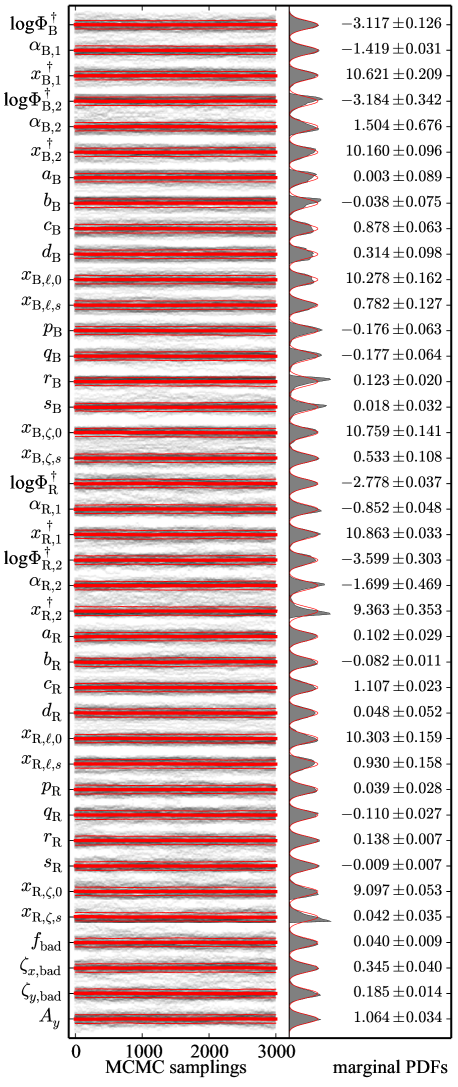
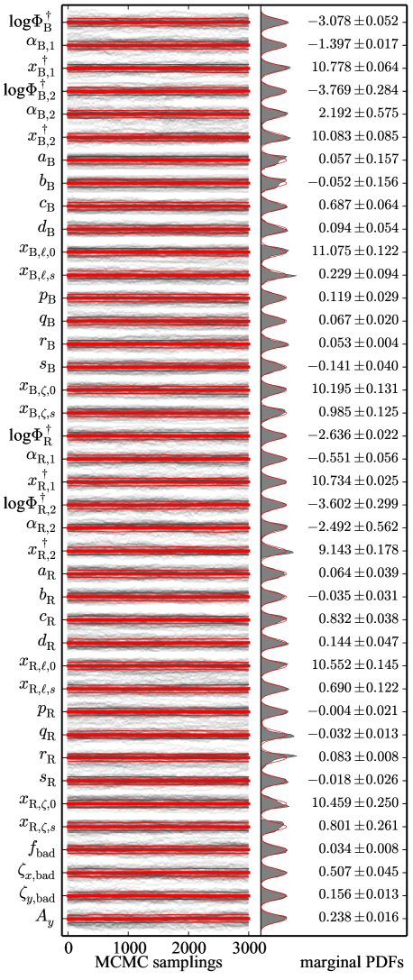
Figure 5: Diagnostic plots showing the convergence of our MCMC fits to the $(g-i)$– and $(g^{*}\!-i^{*})$–$M_{*}$ CMDs (left and right panel, respectively), and a visual table of the fit results— In each panel, the distinct tracks show the values of each of the parameters in the model at individual MCMC steps, for 200 individual walkers. For each parameter, the tracks have been scaled by the mean and RMS over all samplings, so that the each track is centred on ‘the’ fit value, and the width of each track is scaled to match the formal uncertainty in the value of that parameter. The actual fit values for each parameter are given with uncertainties at right; machine readable tables of these results will be published online. The mean and variance in each parameter is shown as a function of MCMC step number as the heavy and thinner lines, respectively. That these lines are flat show that the fits have fully converged. The autocorrelation time for each parameter is in the range 50–150 MCMC steps. We thus have $\gtrsim 4000$ independent samplings of the values of each parameter. Finally, the grey histograms at right show the distribution of parameter values over all MCMC samplings; that is, the shape of the marginalised PDF for each parameter. In all cases, these PDFs can be seen to be well sampled. Further, in most, but not all cases, the PDFs can be seen to be well described by a simple Gaussian (the red curves).

Given the particular parametric form of our model, and given that we have observed our specific dataset, what we want to do is to use the data to constrain the possible values of the parameters in $\mathbf{P}$. In other words, we want to construct the posterior probability density function (PDF) for each of the individual parameters, $P_{n}\in\mathbf{P}$, so that we can evaluate the probability that the parameter $P_{n}$ has the value $P_{n}^{\prime}$; that is, $\mathrm{Pr}(P_{n}=P_{n}^{\prime}|\mathbf{X},\mathbf{S},\mathbf{W})$

This is done using Bayes’ theorem, which can be written as:

$$\mathrm{Pr(model|data)}=\mathrm{Pr(data|model)}\times\mathrm{Pr(model)}~{}.$$ (15)

Here, $\mathrm{Pr(data|model)}=\mathcal{L}(\mathbf{X},\mathbf{S},\mathbf{W}|\mathbf{P})$ is just the scalar likelihood function as defined in Eq. (14), which can only be computed given a full set of values for the model parameters. In contrast, $\mathrm{Pr(model|data)=Pr}(\mathbf{P}|\mathbf{X},\mathbf{S},\mathbf{W})$ is the full, high-dimensional PDF for the values of the parameters $\mathbf{P}$, which is what we are interested in deriving.

Bayes’ theorem links these two quantities via the prior distribution function, $\mathrm{Pr(model)}$, which is an assumed, a priori statement of our expectations for the probability of different parameter combinations with respect to one another. By invoking Bayes’ theorem, we are therefore required to explicitly state our priors on the relative probabilities, $\mathrm{Pr}(\mathbf{P})$, of different values for each of the individual parameters $P_{n}\in\mathbf{P}$.

The decision of what priors to adopt is by no means trivial, but it is also inescapable. All fitting algorithms include priors. One cannot compare the relative likelihoods of two different trial parameter values without an implicit or explicit prior, even if that prior is that the two values are, a priori, equally likely.

In the absence of any clearly better alternatives, we adopt uniform (or uninformative) priors on each of the parameters in $\mathbf{P}$. This includes uniform priors for, for example, the $x^{\dagger}$s, which is equivalent to logarithmic priors for the $M^{\dagger}$s. The exception to this rule is for the slope parameters for the linear relations that go into both $\ell(x^{\prime})$ and $\zeta(x^{\prime})$. Here we take uniform on the angle of the relation; that is, our priors are uniform in, for example, $\mathrm{arctan}~{}a$ and $\mathrm{arctan}~{}p$.

It is worth noting that with this choice of uniform priors, the prior function $\mathrm{Pr(\mathbf{P})}$ is constant, and so $\mathrm{Pr}(\mathrm{model}|\mathrm{data})$ is directly proportional to $\mathrm{Pr}(\mathrm{data}|\mathrm{model})$. With this decision, the Bayesian formalism thus all but reverts to that of traditional, frequentist statistics. In other words, at least in our case, the only difference between the Bayesian and the more familiar frequentist approach is that, as Bayesians, our priors are made explicit.

Formally, the PDF for the single parameter $P_{n}$ is derived by marginalising over all of the other parameters in $\mathbf{P}$; ie:

$$\mathrm{Pr}(P_{n}=P_{n}^{\prime}|\mathbf{X},\mathbf{S},\mathbf{W})\propto\int\mathrm{d}P_{m}~{}\mathcal{L}(\mathbf{X},\mathbf{S},\mathbf{W}|\mathbf{P})~{}\mathrm{Pr}(P_{m}),~{}$$ (16)

where $\mathrm{Pr}(P_{m})$ is constant for uniform priors, and the integral should be understood to be evaluated for all $P_{m}\in\mathbf{P}/\{P_{n}\}$. (Here, the symbol ‘$/$’ means the set complement.) In words, this expression is best understood as a probability weighted integral over all possible combinations of parameter values, with the condition that the specific parameter of immediate interest, $P_{n}$, takes the particular value $P_{n}^{\prime}$.

Note that this formalism also works for any quantity $Q(\mathbf{P})$ that can be deterministically computed from the defining parameters of the model. This includes, for example, the values of the characteristic densities, $\Phi^{\dagger}$, for each of the Schechter functions. This also includes the values of the individual $\Phi(x_{k})$s; i.e., the values of the MFs at any of the discrete $x_{k}$s used to define the model. Here, since $\Phi(x_{k})$ is not a member of the defining parameter set $\mathbf{P}$, the ‘complementary’ parameter set of $P_{m}$s in Eq. (16) is the full set $\mathbf{P}$. In this way, we can derive formal statistical uncertainties on $\Phi(x_{k})$, $\ell(x_{k})$, or $\zeta(x_{k})$ that fully account for any and all covariances between the 40 parameters in $\mathbf{P}$. We will discuss this point in more detail in §7.3.

The fitting of the model thus entails mapping out the scalar likelihood function $\mathcal{L}(\mathbf{X},\mathbf{S},\mathbf{W}|\mathbf{P})$ over the 40-dimensional parameter space defined by $\mathbf{P}$. This is done using the technique of Monte-Carlo Markov Chain (MCMC) sampling. In essence, MCMC is just a random walk through the high-dimensional parameter space. The key to MCMC techniques is that possible steps are considered randomly, but are accepted or rejected probabilistically. More specifically, the chances of a step being accepted are defined by the ratios of the PDF — that is, by the prior-weighted likelihood function — at the present and potential future locations in $\mathbf{P}$-space.

In the first instance, this makes MCMC a very robust means of exploring the parameter space with a view to finding the global maximum of the PDF. In the second instance—once the algorithm has found itself near to the maximally likely solution—MCMC sampling represents an extremely convenient means of sampling the high-dimensional PDF. In this phase of the fitting process, the key to the utility of MCMC sampling is that it is ergodic; that is, the chances of a point in $\mathbf{P}$-space being sampled is directly proportional to the value of the PDF at that point. As a consequence, the distribution of MCMC-sampled points converges to a faithful mapping of the value of the PDF in $\mathbf{P}$ space.

This means that the marginalisation integral in Eq. (16) can be very easily computed to a high level of accuracy by simply taking a histogram of sampled values of any of the quantity. Similarly, the joint PDF for any two (or more) quantities can be computed by taking the two- (or more-)dimensional histogram over those parameters. Further, the marginalisation integral for the ‘most likely’ value of any quantity $Q(\mathbf{P})$—properly speaking, the expectation value for $Q$—can be trivially computed by taking the mean of all MCMC sampled values for that quantity (cf. Eq. (16)); i.e.:

$$\begin{split}\left<Q\right>&\equiv\int\mathrm{d}\mathbf{P}~{}Q(\mathbf{P})~{}\mathrm{Pr}(\mathbf{P}|\mathbf{X},\mathbf{S},\mathbf{W})\\ &\cong\mathrm{mean}\big{[}Q(\mathbf{P}_{i})\big{]},\end{split}$$ (17)

where $\mathbf{P}_{i}$ represents the individual (post-convergence) MCMC sampled sets of trial values for the parameters $\mathbf{P}$. Similarly, the uncertainty on the value of a single parameter can be simply computed as the RMS of MCMC sampled values (i.e., $\sigma_{Q}^{2}=\left<Q^{2}\right>-\left<Q\right>^{2}$), and the joint, covariant uncertainties on multiple parameters can be computed via the Pearson correlation coefficient (i.e., as in Eq. 3).

We have used the publicly available python package emcee (Foreman-Mackey et al., 2012) to actually perform the MCMC fits presented in this work. Compared to the standard Metropolis-Hastings MCMC sampling algorithm, the most important feature of emcee stems from its use of multiple MCMC ‘walkers’ when sampling the parameter space. The step size for individual walkers are based on the distribution of the ensemble of all walkers, using an affine-invariant ‘stretch move’ algorithm, which leads to very efficient sampling, even in the case of strongly anisotropic PDFs. For this work, a key practical advantage of using emcee is that it is trivially parallelisable.

The results of this MCMC fitting process are illustrated in Fig. 5. This figure shows the individual sets of trial values for each of the 40 parameters in $\mathbf{P}$ for unique MCMC samplings. These samplings are, in a sense, our results—they represent the high dimensional PDF for the values of the parameters in $\mathbf{P}$.

For clarity, the tracks for individual parameters in Fig. 5 have been scaled according to the mean and RMS values of the thinned and post-burn MCMC samplings; that is, according to the Bayesian estimator for the most likely value, and the uncertainty in that value. These values are given in each panel of Fig. 5; this Figure thus also serves as a table of the results of our fits. The fact that each of these lines is horizontal shows that the fits have in fact converged.

To the extent that the PDF for any given parameter value is truly Gaussian, these values can be used to fully describe the PDFs. Again, the distribution of MCMC samplings converges to a faithful mapping of the PDF, with no embedded assumptions of Gaussianity; these distributions are shown in Fig. 5 as the grey histograms. In all cases, the PDFs can be seen to be well-sampled. Further, in most—but not all—cases, the PDFs can be seen to be well described by a simple Gaussian. Again, we stress that these distributions naturally and fully account for covariances among the values of (many) different parameters.

5.3 Model Selection and the Limits of Objectivity

5.3.1 Model Selection

How can we be satisfied that, for example, the B population really is (or is not) better described by a double- rather than a single-Schechter mass function, or whether or not the blue CMR can be adequately described using just a simple linear relation? To explore these kinds of issues, we have made many fits to our dataset, in which we have eliminated one or more of the 40 parameters that go into our most general model. Our tests have been systematic, but by no means exhaustive. As described below, we have used these tests to ensure that we are not grossly overfitting the data.

There are a number of Bayesian approaches to the problem of model selection which we have explored: the Bayes factor, $K$, the closely related Akaike and Bayesian Information Criteria (AIC and BIC, respectively), and the Deviance Information Criterion (DIC). While these different approaches are each based on slightly different assumptions, and are thus strictly valid in slightly different circumstances, they can all be thought of as being similar in spirit to a traditional frequentist log-likelihood-ratio test. In asymptotic limits, AIC $\approx$ BIC $\approx$ DIC $\approx-2\ln K$. A difference of 2.5 (or 10) in the IC of two different models implies a likelihood ratio of $\approx$ 3.5 (or 150), where the model with the lower value for the IC is the preferred one. However, unlike a simple likelihood ratio test, each of these quantities includes an explicit or implicit penalty for larger numbers of parameters, so as to protect against over-fitting of the data.

We have focussed primarily on the AIC and BIC, which are defined with reference to the maximum of the likelihood function, $\mathcal{L}_{\mathrm{max}}$. Since extra parameters can only increase the value of $\mathcal{L}_{\mathrm{max}}$, the question is whether or not this improvement is sufficient to merit the inclusion of an extra parameter. The penalty terms for additional parameters for the AIC and BIC are $2k$ and $k\ln n$, respectively, where $k$ is the number of free parameters in the model, and $n$ is the number of data points. Thus it can be seen that, all else being equal, the BIC penalises additional parameters more strongly than the AIC for $n\gtrsim 8$. (In our case, $\ln n\approx 10$, so the BIC penalty is roughly 5 times larger.)

In other words, the BIC prefers models with fewer parameters. Thus, where the BIC disfavours a simpler model, this model is definitely too simple, and should not be used. Conversely, the AIC prefers models with more parameters. Where the AIC disfavours a model with more parameters, then that the use of that model is definitely overfitting the data.

In order to ensure that we are not abusing our data, we have used these two information criteria to explore the consequences of omitting individual parameters from the model described above. Given the number of parameters that go into our general model in its most general form, it is impractical to do this in a properly exhaustive way. Instead, starting from the most general form of our model, we have considered omitting individual parameters one at a time to see whether or how our model might be simplified.

First, we have tried successively omitting the parameters $c$, $d$, $r$, and $s$ (i.e., the parameters that describe the step or bend in the locus of or scatter around the CMRs). When fitting to the $(g-i)$ CMD, it is possible that a simpler description of the B CMR is possible: omitting the parameters $c{}_{\mathrm{B}}$ and $d{}_{\mathrm{B}}$ improves both information criteria by 8 and by 10, respectively. While this constitutes positive statistical evidence against the need for one of these parameters, it is ambiguous which one should be excluded. When fitting to the $(g^{*}\!-i^{*})$ CMD, the results are similar. Based on the BIC, it is preferable to omit either $r{}_{\mathrm{R}}$ or $s{}_{\mathrm{R}}$ (but not both), and also possibly and $d{}_{\mathrm{B}}$ and $b{}_{\mathrm{R}}$ ($\Delta$BIC = 8 for both).

The ambiguity in these results make perfect sense looking at the table of results given in Fig. 5. These parameters which may or may not be necessary are those whose fit values are statistically consistent with being zero. Their inclusion or exclusion thus makes little if any difference to the fits, and the decision as to whether or not to include these parameters has no practical consequences.

We therefore elect to use the most general description possible for the locii of and scatters around the CMRs, by fitting for all of these parameters. In this sense, our results can be thought of as hypothesis testing the need for each of the $c$s, $d$s, $r$s and $s$s. Where the fit values for any of these parameters are consistent with zero, then that parameter may be unnecessary for a good description of the data. These results nonetheless encapsulate positive information about the forms of locii of and scatters around the B and R CMRs.

Perhaps more interesting is what happens when we trial alternate descriptions of the MFs. As well as the general double Schechter parameterisation, we have trialled a coupled twin-Schechter description, where the two Schechter functions that describe either the R or B population have the same characteristic mass (i.e., $x^{\dagger}_{2}=x^{\dagger}_{1}$). We have also trialled using only a single Schechter function (i.e., $f_{2}=0)$.

When fitting to the $(g-i)$ CMD, the BIC definitely disfavours a single Schechter function description for the B MF ($\Delta$BIC $\gtrsim 30$), indicating that such a model definitely underfits the data. The BIC also definitely disfavours the coupled, twin Schechter function description for the B MF; the data definitely prefer a double Schechter function description of the B MF, with $x^{\dagger}{\mathrm{B},2}\neq x^{\dagger}_{\mathrm{B},1}$. At the other extreme, the AIC disfavours the most general, double Schechter model ($\Delta$AIC $\lesssim 6$; odds $\approx$ 20:1) for the R MF described. That said, it is worth noting that both the AIC and BIC (weakly) prefer a single Schechter description for the R MF. This may not be surprising, given how weakly constrained the values of $\alpha_{\mathrm{R},2}$, and $x^{\dagger}_{\mathrm{R},2}$ are.

When fitting to the $(g^{*}\!-i^{*})$ CMD, the BIC disfavours a single Schechter MF for the R population ($\Delta$BIC $\lesssim 10$). The BIC does not obviously prefer the more complicated, independent double Schechter descriptions of either the B or R MFs; the coupled, twin Schechter functions are just as good. The variation of the model that best balances between the two criteria is the one that uses coupled, twin Schechter functions to describe both the B and the R MF.

In light of all of the above, we will continue our analysis using the most general form for our model, which is fully defined by 40 parameters. This is despite the fact that both the AIC and BIC prefer a single Schechter description for the R MF when analysing the $(g-i)$ CMD. (But of course, this being the case, the fits do not make use of the additional freedom that the second Schechter component provides, precisely because it is not necessary for a good description of the data.) In this sense, our fit results can be taken as limiting the deviations from Schechter-ness in the observed MF for R type galaxies.

For all of the rest, we can say that we are not definitely overfitting the data, nor are we definitely underfitting the data. Beyond this point, however, all we can say is that we have done the best that we know how (and monopolised 64 cores for more than 2 months) to ensure that we are using the best and simplest model that we can to describe the existing data.

5.3.2 The Limits of Objectivity

In some of the above, there is some ambiguity, inasmuch as the data do not provide strong evidence for or against the inclusion of some parameters. This is particularly true for whether or how the B and R MFs should be described with a combination of Schechter functions. To the extent that there is ambiguity, our decisions about whether or not to include these parameters are subjective, hence arbitrary.

To the extent that these points are ambiguous, however, they are also unimportant. This is true in the sense that these decisions have no strong impact on the statistical quality of the fits to the data. This is also true in the sense that the best fit models based on the less-general parameterisations provide essentially identical results.

What we have done in the above is to explore special cases or restricted classes of the general form of our model. The question that naturally arises is whether there are some alternative parameterisation might provide a better description of the data. For instance, it could be that a Lorentzian or a Student’s $t$ or a skewed Gaussian description of the scatter around the CMRs yields a better statistical description of the data. Of course, a properly exhaustive search of all conceivable models is impossible.

This brings us to the final and most important caveat on our results. While the formal statistical uncertainties on our CMR and MF fits are impressively small, the values themselves cannot but be determined by the decisions made in constructing the parameterised, descriptive model that has been used. On the other hand, the same criticism can be levelled at any model or modeller—even a fully physically-minded explanatory model is forced to presuppose the validity of the theoretical framework on which it is based. At this level, some degree of subjectivity is inescapable.

Once we have set the parametric form of our descriptive model, however, it is then left to the data to decide on the particular parameter values that provide the best description, including all the characteristics of the B- and R- populations. That is, given our choice of parameterisation, it is the data themselves that define the bimodal distributions. The results of this modelling thus provide objective B/R classifications insofar as objectivity is possible. These results can thus be said to provide an accurate, reliable, and robust phenomenological description of the observed data—and this is all that we have set out to obtain.

6 Results I. — The bivariate colour–mass distributions

6.1 Demonstrating the quality of the fits

In order to illustrate our ability to perform such a detailed descriptive modelling of the data, as well as the quality of the resultant fits, consider Fig. 6 and Fig. 7. Our task in this section is to describe and discuss these Figures. Building on the discussion begun in §4, we will also flag the major issues with, and caveats on, the interpretation of our results, which should be kept in mind in all that follows.

Fig. 6 and Fig. 7 show the $(g-i)$ and $(g^{*}\!-i^{*})$ CMDs, respectively. In each panel, we have split our sample up into bins of $\log M_{*}$, each with width 0.2 dex. The solid black histograms then show the incompleteness-corrected colour distributions within each of these mass bins: the lowest histogram is for the $8.7<\log M_{*}<8.9$ bin, the next is for the $8.9<\log M_{*}<9.1$ bin, and so on. The normalisation of each of these histograms is arbitrary, but is the same for all bins in both Figures.

Illustrative statistical uncertainties in the observed colour distributions are shown by the black error bars. These uncertainties have been estimated using bootstrap resampling. (We have not attempted to account for field–to–field variance due to large scale structure.) For $\log M_{*}\gtrsim 9.5$, these statistical uncertainties are negligible. Further, even for the lowest $8.7<\log M_{*}<8.9$ bin, the statistics are reasonably good. Particularly for $9\lesssim\log M_{*}\lesssim 11$, then, there should be no question as to whether or not the data are good enough to allow an independent double-Gaussian (or some other parametric) fit to any or all of the individual, mass-binned colour distributions.

The smooth curves in Fig. 6 and Fig. 7 show the results of our descriptive modelling of the bivariate $(g-i)$ and $(g^{*}\!-i^{*})$ colour-mass distributions. The red and blue curves show the distinct R and B components of the model; the black curve is the total, R–plus–B distribution. Note that for these illustrative purposes, we have convolved the modelled colour-distributions with typical $(g-i)$ or $(g^{*}\!-i^{*})$ uncertainties for each mass bin, so that these curves are directly comparable to histograms for the observed data.

Before moving on, let us stress that we have not binned the data in the course of fitting it: the binning in mass and colour in these figures is for illustrative purposes only. Further, nowhere in the modelling is it ever specified—or even relevant—whether any particular galaxy belongs to either the R or the B populations; there is no binning in this sense either.

If, for example, we were to just fit double Gaussian distributions to the observed colour distributions for the distinct mass bins that are shown in Fig. 7, then the inferred values for the centres, scatters, and normalisations of the R and B distributions in each bin would be completely independent. Given the relatively poor sampling for $\log M_{*}\lesssim 9.3$ and $(g^{*}\!-i^{*})\gtrsim 0.7$ galaxies, we would have no means of robustly constraining the properties of either of the two Gaussian components of the $(g^{*}\!-i^{*})$ colour distributions for these very low masses—or even whether or not two Gaussian components should be used.

But this is not what we have done. In effect, we have assumed that the centres, scatters, and normalisations of the (Gaussian) B and R colour distributions vary smoothly as a function of mass. In this sense, the derivation of each and every of the individual modelled B and R colour distributions shown in Fig. 7 is based on each and every datapoint that we have.

Ultimately, all the model considers is the relative probability of finding a galaxy—irrespective of type—at a particular point in the colour–mass plane. In other words, we are using a mixture model of two distinct but overlapping populations to describe the joint colour–mass distribution function of all galaxies—we are fitting for the 2D scalar function that is represented in Fig. 6 and Fig. 7 as the black curve. In this way, we are able to characterise the CMRs and MFs of the two populations without ever explicitly considering which galaxies belong to which population.

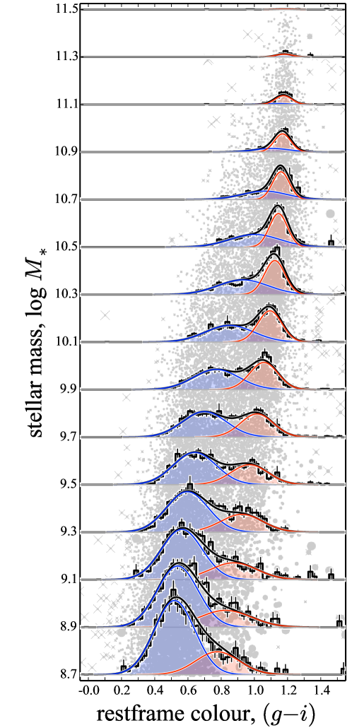
Figure 6: Demonstrating the quality of our fits to the joint $(g-i)$–$M_{*}$ distribution.— The histograms in this Figure show the observed $1/V_{\mathrm{max}}$-weighted distribution of restframe $(g-i)$ colours of $z<0.12$ galaxies, computed in bins of $\log M_{*}$ centred on $\log M_{*}$ = 8.8, 9.0, …, 11.4. The errorbars show the statistical uncertainties on each these distributions, derived by bootstrap resampling. The smooth curves show the results of our modelling: the blue and red curves show the fit distributions for the B- and R-populations; the black curves shows the net B+R distributions. Underlaid beneath all this, the grey points show the data themselves. The size of each point is proportional to $1/V_{\mathrm{max}}$. Data objectively classified as being ‘bad’ are marked with a cross. Note that we have not binned the data in the course of the fits; the binning in this Figure is for illustrative purposes only. It is clear that the fit model provides a good description of the observed data.

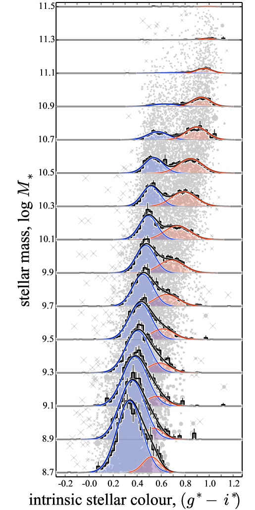
Figure 7: Demonstrating the quality of our fits to the joint $(g^{*}\!-i^{*})$–$M_{*}$ distribution.— The histograms and smooth curves in this Figure show the observed and fit distributions of intrinsic $(g^{*}\!-i^{*})$ colours in bins of $\log M_{*}$; all symbols in this Figure and their meanings are analogous to Fig. 6. In contrast to Fig. 6, the general galaxy population is better separated into distinct R and B populations on the basis of $(g^{*}\!-i^{*})$ than of $(g-i)$, in the sense that there is less overlap between these two distributions in this Figure than in Fig. 6. Further, as in Fig. 6, we see no compelling evidence for the need to include a third, ‘green’ population. In comparison to Fig. 6, the need for a multiple-Gaussian description of the observed colour distributions for $\log M_{*}\lesssim 9.3$ is less clear; this point is discussed in detail in §6.2. In any case, as in Fig. 6, the fit model can be seen to provide an excellent description of the observed data.

6.2 What could possibly go wrong? The R population at low masses

While our parametric model does provide a very good description of the data, a good description is not necessarily the same as the right one (see related discussions in §5.3.2 and §9.3). Other parameterisations of the colour distributions (at fixed mass) are possible, and may lead to different results — but this is always true. The fact that the answer we get depends on how we have devised our analysis is inescapable. If our assumptions, which are clearly stated and motivated in §4.4 and §10, are shown to be invalid, then our results go with them. Indeed, we have gone to great lengths to make this point in §4. Without denying these inescapable truisms, the fact remains that our model does provide a very good description of the data, and so offers one potential avenue for understanding the data.

At least for $\log M_{*}\gtrsim 9.7$, the model does perform its intended function: decomposing the observed data into a mixture of two populations, which are distinguished and defined by their own distributions of colours, which we take to be a tracer of the constituent stellar populations.

The skeptical reader’s eye may be drawn to the fits at $\log M_{*}\lesssim 9$, however, where the suitability of a double Gaussian fit becomes increasingly problematic. Certainly, in both Fig. 6 and Fig. 7, below $\log M_{*}\sim 9.3$, it becomes difficult for us to claim that we have robustly separated the general galaxy population into two distinct R- and B-populations. How then should one interpret our results at these low masses?

Considering this problem from the modelling perspective, we should ask what aspects of the data drive the fits most strongly. Clearly, it is the shape and normalisation of the B colour distributions that are the best constrained at these low masses. Also, from the nature of the fits, it should be clear that the fits to the B colour distributions are decided primarily by the $(g-i)\lesssim 0.6$ or $(g^{*}\!-i^{*})\lesssim 0.3$ data. Bluewards of the peak of the observed colour distributions, the data are well described by a Gaussian. Then, since the colour distributions for each population are assumed to be symmetric, it is left to the R population to accommodate whatever asymmetries there are in the observed colour distributions.

From a more astrophysical perspective, then, what matters is the extent to which the colour distribution for the B population is expected to be symmetric. However, this will certainly not be the case for $(g-i)$, where the asymmetric effect of dust is expected to skew the B colour distribution to the red. In this case, one would expect the inferred number of R galaxies to absorb some of the reddest B-type galaxies. Indeed, looking at the lowest two or three bins of Fig. 6, one can see immediately how such a description might work.

Rather than trying to fit for an asymmetric or skewed $(g-i)$ distribution (which would be considerably computationally more complicated), we can look at the $(g^{*}\!-i^{*})$ distribution, where we have tried to remove dust as a complicating factor. But looking at the lower three bins in Fig. 7, there is no way to decide whether the slight asymmetry of the observed colour distribution ought to be interpreted as an indication of a separate population, or instead as nothing more than a slight asymmetry in the $(g^{*}\!-i^{*})$ colour distribution of the B population.

Our conclusion is therefore that at these low masses, the (field) red sequence dissolves into obscurity—we no longer see clear evidence of two distinct populations in the $(g-i)$ or $(g^{*}\!-i^{*})$ colour distributions for $\log M_{*}\lesssim 9.5$. (As we have argued in §3, we do not believe that the apparent dearth of low mass red galaxies is due to incompleteness.) Instead, we present our inferred MFs for R-type galaxies as an upper limit on the number densities of galaxies that have moved (or are moving) away from the colour distribution that describes most low-mass galaxies; i.e., the B population.

Again, the fact that the inferred B- and R- populations have substantial overlap serves to underline the subtleties involved in interpreting our results in concrete, astrophysical terms. In particular, even at intermediate masses, it would be unwise to blithely equate the R population with ‘quenched’—but recognise how much more problematic it is to apply the term ‘quenched’ to the hard-cut ‘red’ samples discussed in §4.

6.3 What we have (and have not) done

To sum up: using the parametric model described in §5, we have derived a very good description of the observed bivariate distributions between both $(g-i)$ and $(g^{*}\!-i^{*})$ and stellar mass. This analysis is intended to provide a phenomenological description of the essential characteristics of the bivariate colour–mass distributions. Such a description clearly requires (at least) two populations with their own distinct CMRs and MFs. Our approach enables us to simultaneously and self-consistently describe the bivariate colour-mass distribution functions of the two populations; indeed, this is how these populations are defined.

Again, we stress that the designations B and R refer primarily to the two populations, rather than to individual galaxies. That is, instead of characterising the demographics of galaxy samples that are pre-selected to be ‘blue’ or ‘red’, what we have done is decompose the full population into a mixture of two distinct, but overlapping, subpopulations; we dub these two populations ‘B’ and ‘R’. In this way, we can derive an operational definition for the terms ‘R-type’ and ‘B-type’.

Once this is done, however, it is possible to use these fits to quantitatively—if probabilistically—classify individual galaxies according to the chances that the galaxy in question has been drawn from either the B or R population; i.e., the relative contributions of the B- and R-populations to the data density at any given point in the CMD. (See §7.2, below.) But it is important to understand that these classifications follow from the fits: during the fitting process itself, the B-ness or R-ness of any particular galaxy is irrelevant.

We make no pretensions, however, about providing an explanatory model for the observations. That is, we justify our splitting of the general population into B and R components on the grounds that these are distinctions that galaxies somehow care about. In this way, we derive a phenomenological description of the bimodal—better, the two population—character of the galaxy population, in terms of galaxies’ stellar populations.

The underlying physical differences in the origins and natures of the B- and R-populations, as well as those responsible for the observed ranges of $(g^{*}\!-i^{*})$ colours within each population, remain to be determined (but see §9.2), and will be the focus of future works in this series.

7 Results II. — The Mass Functions and Colour–Mass Relations for Red and Blue Galaxies

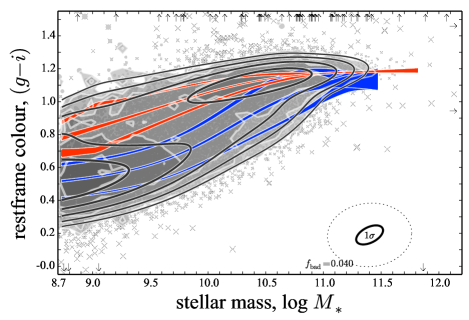
Figure 8: Results of our fits to the restframe $(g-i)$ CMD, highlighting the CMRs for the B and R populations.— This Figure is discussed at length in §7.1. In this Figure, the points show the data. As in Fig. 6 the size of each point reflects the value of the $1/V_{\mathrm{max}}$ weighting for incompleteness, and the crosses show those datapoints objectively identified and censored as ‘bad’. The small arrows show where galaxies fall outside the plotted range. The filled greyscale contours show the incompleteness-corrected data density, in steps of powers of 2. These should be compared to the smooth line contours, which show the bivariate distribution function from our fits. For illustration purposes, these have been convolved with the typical observational errors, shown at the bottom right. Here, the dotted ellipse shows the inferred errors for ‘bad’ galaxies. The main feature of this plot are the smooth curves, which show our fits for the locii of, and scatter around, the $(g-i)$ CMRs for the distinct R- and B-populations. The width of these lines show the 68 % confidence intervals on the values of these functions, as a function of mass, and including all convariances between model parameters. This figure should be contrasted with Fig. 9.

In Fig. 6 and Fig. 7, we have illustrated the quality of our fits to the bivariate $\log M_{*}$–$(g-i)$ and $\log M_{*}$–$(g^{*}\!-i^{*})$ distributions for our sample of $\log M_{*}>8.7$ and $z<0.12$ galaxies. Our task in this section is to lay out the actual fit results—i.e., the CMRs and MFs for R- and B-type galaxies—which describe the two populations. Fit results are given in a machine readable table as additional online material.

7.1 Scaling Relations

The results of our fits for the $(g-i)$ and $(g^{*}\!-i^{*})$ CMRs are shown in Fig.s 8 and 9, respectively. In both of these Figures, the grey points show the data themselves. As in Figures 2, 6, and 7, the size of each point has been chosen to reflect the value of the $1/V_{\mathrm{max}}$ weighting factor. Further, as in Figures 6 and 7, each individual datapoint is marked with a black cross, the size of which has been chosen to reflect the probability that that datapoint has been drawn from the ‘bad’ distribution. The marked points have thus been objectively identified as outliers; they make little to no contribution to the fit CMRs shown. This objective censoring can be seen to be very effective.

The semi-transparent filled contours in Fig. 8 and Fig. 9 show the observed, $1/V_{\mathrm{max}}$-weighted bivariate data density; these contours have the same log₂ scaling as those in Fig.s 1–4. These should be compared to the smooth line contours, which are interlaid between the data points and the fit CMRs, and which show the logarithmic probability density contours from the model. As for Fig. 6 and Fig. 7, to generate these contours, we have convolved the model fits with typical uncertainties, so that these contours are directly comparable to those for the data themselves. These contours thus reflect the combination of the mass functions and the CMRs for these populations. These contours are included mostly for illustration; the mass functions themselves are shown in Fig.s 12 and 13, and are described separately below. The models provide very good descriptions of the observed bivariate $(g-i)$ and $(g^{*}\!-i^{*})$ colour-mass distributions.

In each figure, the smooth lines show the fit locii for the two CMRs, as well as the fits for the RMS scatter around each CMR. The width of each of these lines shows, at fixed mass, the 68 % confidence intervals for each quantity. These uncertainties can be seen to behave reasonably: they are very small where the data concentration is high (e.g., the centres of the red sequences), and become large where the data concentration is low (e.g., the very high mass ends of both the red and blue sequences). In connection with our discussion in §6.2, note how the uncertainties in the locations of the $+1\sigma$ point of the R $(g^{*}\!-i^{*})$ distributions are less than that of the locus of the CMR, which are in turn smaller than those of the $-1\sigma$ point. This again shows how the descriptions of each population are constrained principally by the outer edges of the colour distributions, as well as illustrating how our Bayesian approach can yield meaningful uncertainties on secondary aspects of the model (e.g., the CMRs) that nicely and naturally propagate all the relevant uncertainties in the defining parameters of the model.

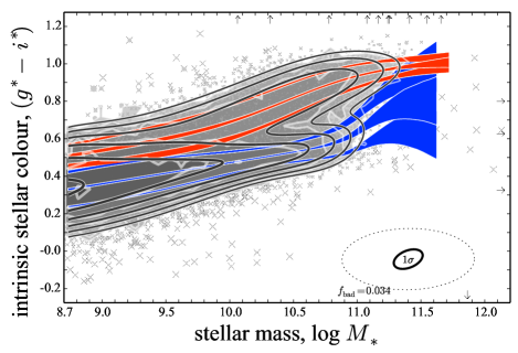
Figure 9: Results of our fits to the intrinsic $(g^{*}\!-i^{*})$ CMD highlighting the CMRs for the B and R populations.— This Figure is discussed at length in §7.1. All symbols and their meanings are analogous to Fig. 8. In comparison to the $(g-i)$ CMD, we make the following qualitative observations. The ‘blue sequence’ in this $(g^{*}\!-i^{*})$ CMD is both tighter and more linear than the $(g-i)$ ‘blue cloud’. This implies that the upturn in the ‘blue’ CMR seen in Fig. 8 is caused by a change in the dust properties of blue galaxies with $9.5\lesssim\log M_{*}\lesssim 10.5$, rather than a change in the stellar populations of these galaxies. Note how the $\log M_{*}\gtrsim 10.8$ upturn to the B CMR in this Figure coincides with the convergence between the $(g-i)$ CMR for the two populations in Fig. 8. The rather steeper slope of the R-type CMR the shows how this population is less homogenous than the B-population: lower mass R-type galaxies have rather different stellar populations to their higher mass cousins. At the same time, the relatively tight and smoothly sloping CMR show how across the R-type population, mass is a relatively good predictor of stellar population, suggesting a common evolutionary pathway for these galaxies. These points are discussed further in §8.

In Fig. 8, there is an upturn to the B CMR that begins around $\log M_{*}\sim 9.7$. As expected from Fig. 1, the behaviour seen in Fig. 9 is rather different: what is seen in the $(g-i)$ CMD as the blue cloud is seen in the $(g^{*}\!-i^{*})$ CMD as a considerably tighter and more linear blue sequence. This implies that the slope of the $(g-i)$ CMR in Fig. 8 for the B population is more a product of increasing dust obscuration in higher mass galaxies, rather than differences in the colours of the underlying stellar populations.

At the very end of this $(g^{*}\!-i^{*})$ blue sequence, there is the hint of an upturn to redder $(g^{*}\!-i^{*})$ colours for $\log M_{*}\gtrsim 10.8$, but this is where the uncertainties become large. Intriguingly, looking at Fig. 8, the B CMR becomes indistinguishable from the R one in the $(g-i)$ CMD at this mass range: the locii of the two CMRs converge, and the scatter in the B CMR becomes small. That is, the B population becomes indistinguishable in the apparent $(g-i)$ CMD for $\log M_{*}\gtrsim 10.8$. Further, those $\log M_{*}\gtrsim 10.8$ B-type galaxies identified in the intrinsic $(g^{*}\!-i^{*})$ CMD have rather different stellar populations to the rest of the blue sequence.

Turning to the R population, the most remarkable aspect of the $(g-i)$ CMD (Fig. 8) is how the $\log M_{*}\gtrsim 10.5$ R CMR flattens and tapers to have essentially no intrinsic scatter. These are the galaxies that one might expect to be truly ‘red and dead’. Below this mass, the $(g-i)$ CMR for the R population bends to bluer colours for lower masses. The $(g^{*}\!-i^{*})$ CMR shows slightly different behaviour: here, the stellar populations of R-type galaxies become very gradually redder across the range $9.5\lesssim\log M_{*}\lesssim 10.8$.

Taking the results shown in Fig. 9 at face value, the simplest interpretation would be that the R-type galaxies are moving towards the ‘dead sequence’ only slowly, and in such a way that creates or preserves a relatively tight relation between a galaxy’s mass and its stellar population. In this scenario, the higher mass galaxies would appear to have progressed further in this long migration. We will expand further on the simple observations above in §8.

7.2 Objective classification, following from the fits

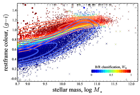
Figure 10: Illustrating our objective B/R classifications, based on the restframe $(g-i)$ colour–mass diagram.— This Figure is discussed in detail in §7.2. There are two main features to this Figure. First, the smooth line contours show the bivariate distributions for the B and R components of the models, using the same logarithmic scale as in earlier plots. This information can be used to classify individual galaxies according to the probability that they have been drawn from one or the other population. Individual points in this Figure are colour-coded according to these classifications, $W{}_{\mathrm{R}}$. Given the empirical fact of scatter in both the blue cloud and the red sequence (see Fig. 6), and thus the overlap between the two populations, the individual classifications can be ambiguous, particularly at high masses. For example, a galaxy observed right on the locus of the red sequence still has a $\sim 20$–25 % chance of having come from the bluer B-population.

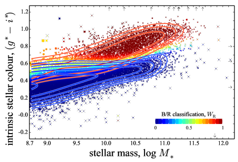
Figure 11: Illustrating our objective B/R classifications, based on the intrinsic $(g^{*}\!-i^{*})$ colour–mass diagram.— All symbols and their meanings are analogous to Fig. 10. Note how, particularly at higher masses, the R-population is more unambiguously distinguished in the $(g^{*}\!-i^{*})$ CMD than the $(g-i)$ CMD shown in Fig. 10; only a small fraction of galaxies have ambiguous classifications (i.e., intermediate values of $W{}_{\mathrm{R}}$). As discussed in §7.2 and §7.3, this means that our empirical determinations of the MFs for B/R classified galaxies are not strongly dependent on the quality of our fits. At lower masses, and particularly around $\log M_{*}\sim 9.5$, the populations are inferred to overlap to the extent that up to $\sim 20$ % of galaxies in the blue sequence are members of the R population. The overlap between the two populations in this Figure, as well as Fig. 10 demonstrate the importance of accounting for scatter around the CMR when characterising the two populations.

In Fig. 10 and Fig. 11, we re-present the results of our fits to the $(g-i)$ and $(g^{*}\!-i^{*})$ CMDs in a different way, in order to illustrate how these fits can be used to develop an objective, quantitative B/R classification scheme for individual galaxies. In essence, the idea is to give each galaxy a score, which encapsulates the relative probability, based on our fits, that that galaxy has been drawn from the R-, B-, or even the ‘bad’ population.

The R-type score, $W{}_{\mathrm{R}}{}_{,i}$ is given by the relative number of R-type galaxies expected to be found at the location $\underline{x}{}_{i}$, after convolving the fit models with the observational uncertainties encapsulated within the covariance matrix $\underline{\underline{\mathrm{S}}}{}_{i}$. Formally, and using the notation and definitions introduced in §5.1, these values are computed as:

$$W{}_{\mathrm{R}}{}_{,i}(\underline{x}{}_{i},\underline{\underline{\mathrm{S}}}{}_{i}|\mathbf{P}_{\mathrm{fit}})\equiv\mathcal{L}{}_{\mathrm{R}}{}_{,i}(\underline{x}{}_{i},\underline{\underline{\mathrm{S}}}{}_{i}|\mathbf{P}_{\mathrm{fit}})/\mathcal{L}{}_{i}(\underline{x}{}_{i},\underline{\underline{\mathrm{S}}}{}_{i}|\mathbf{P}_{\mathrm{fit}})~{}.$$ (18)

Here, $\mathbf{P}_{\mathrm{fit}}$ is the set of fit-for values for the parameters $\mathbf{P}$, and $\mathcal{L}{}_{\mathrm{R}}{}_{,i}(\underline{x}{}_{i},\underline{\underline{\mathrm{S}}}{}_{i}|\mathbf{P}_{\mathrm{fit}})\equiv p{}_{\mathrm{R}}(x{}_{i}|\mathbf{P}_{\mathrm{fit}})\otimes\mathcal{G}_{2}(\underline{x}{}_{i},\underline{\underline{\mathrm{S}}}{}_{i})$. And of course $W{}_{\mathrm{B}}$ and $W{}_{\mathrm{bad}}$ can be defined/computed in an analogous way, so that $W{}_{\mathrm{B}}+W{}_{\mathrm{R}}+W{}_{\mathrm{bad}}=1$.

We illustrate how these classifications work in Fig. 10 and Fig. 11. In these Figures, the data have been colour coded according to their particular values of $W{}_{\mathrm{R}}$. Note that, because these classifications depend on the measurement uncertainties as well as the measured values themselves, there can be some variation in the $W{}_{\mathrm{R}}$s for galaxies with very similar colours and masses.

Note how, particularly at higher masses ($\log M_{*}\gtrsim 10$), there is considerably less ambiguity in the classifications based on the $(g^{*}\!-i^{*})$ CMD, in comparison to those based on the $(g-i)$ CMD. As can be seen in Fig. 10, the B and R populations overlap in the $(g-i)$ CMD to the extent that, even along the locus of the R CMR, $\sim 10$-15 % of galaxies come from the B population (see also Fig. 6). Note, too, how the situation is reversed for $\log M_{*}\lesssim 10$. The point to be made here is that, where there is substantial overlap between the two populations, it is not possible to unambiguously determine whether a particular galaxy is a member of the R or the B population without some additional information.

It is a legitimate question to ask what additional information could or should be used to refine these classifications. While it may be tempting to incorporate morphological or structural information—Sérsic index, $n$, for example— into the ‘red’ selections, we note that this would result in a sample of ‘red and high-$n$’ galaxies, rather than a sample of ‘red’ galaxies. (See Kelvin et al., 2014, for a detailed discussion of this problem.) In this sense, there is the very real danger that inclusion of additional parameters makes things more confusing, rather than less. We will explore this issue further in future papers in this series.

In this context, we note that these objective, quantitative classifications can also be cast as weights, which can be useful in studying the properties of R- and B-type galaxy samples. Fig. 10 and Fig. 11 can thus be alternatively understood as illustrating a ‘soft’ red/blue selection scheme, which is a smooth function of mass and colour. This scheme naturally accounts for the scatter around the R and B CMRs, as well as the R/B fraction, as a function of mass. It also fully accounts for photometric scatter, due to error/uncertainties in the measurements themselves.

This Figure thus helps show how our ‘B-’ and ‘R-type’ designations are qualitatively different to simple ‘blue’ and ‘red’ colour selections. As discussed in detail in §9.1, below, this is the crucial point that explains why our determinations of the MFs for the B and R populations differ strongly from those for ‘blue’ and ‘red’ galaxies given by previous authors.

7.3 The mass functions

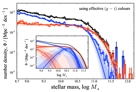
Figure 12: The mass functions for the B and R galaxy populations, as derived from our fits to the restframe $(g-i)$ CMD.— The smooth blue and red curves show the fit mass functions for the B and R populations; the black curve shows the net B–plus–R mass function. The inset panel shows the two separate Schechter components that go into each of the B and R MFs. The solid lines in this inset show ‘the’ fit MFs; the shaded regions show the 68 and 99 % confidence intervals for each component. The uncertainties on the total B and R MFs are shown in the same way in the main panel. Although the individual Schechter components are partially degenerate, the overall MFs are very well constrained. Except for the highest masses, the uncertainties are comparable to the width of the lines used to show the fits, and so are difficult to see. For comparison to the fit results, the blue and red histograms show the empirical MFs, where individual galaxies have been weighted by their values of $W{}_{\mathrm{R}}$ or $W{}_{\mathrm{B}}$. The curves are not fit to the histograms; instead, the histograms are derived using the quantitative classifications that come from the fits.

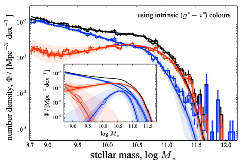
Figure 13: The mass functions for B and R galaxy populations, as derived from our fits to the intrinsic $(g^{*}\!-i^{*})$ CMD.— In contrast to Fig. 12, this Figure shows the mass functions for the R and B populations as inferred from the $(g^{*}\!-i^{*})$, rather than the $(g-i)$, CMD; otherwise, all symbols and their meanings are the same as in Fig. 12. Note that we do not consider the apparent low mass upturn in the R MF to be robust, for the reasons given in §6.2, and §7.3 (see also Fig. 7). Further, there is not conclusive statistical evidence that a second Schechter component to the R MF is required §5.3. The quantitative discrepancies between the results shown in this Figure and in Fig. 12 for $\log M_{*}\lesssim 10$ can be understood looking at the distributions shown in Fig. 6 and Fig. 7. The implication from this Figure and Fig. 12 is that systematic uncertainties in the low-mass values of the R MF are at least a factor of 2. It is worth stressing, however, that the two sets of results agree at the $\lesssim 2\sigma$ level for all $\log M_{*}\gtrsim 10$. Compared to previous results, we find that the B-population—i.e., galaxies with young stellar populations—extends to much higher masses, and we find considerably fewer ‘old’ galaxies at lower masses. (see also Fig. 14).

The inferred MFs for the R and B populations, based on the $(g-i)$ and $(g^{*}\!-i^{*})$ CMDs, are shown in Fig. 12 and Fig. 13, respectively. In the main panels, the solid lines show our fits for the mass functions when fitting the model as described in §5. The heavier and lighter shaded regions around each line show the 68 % and 99 % confidence intervals for each mass function. Note that these are only visible at the highest masses, and at the low-mass end of the R MF. Elsewhere, the formal statistical uncertainties in the fits are smaller than the width of the lines.

In both cases, the results shown in these figures involve implicit marginalisation/averaging over all possible permutations of counting each individual galaxy as being either B- or R-type. It is true that, in general, we cannot necessarily say with absolute confidence whether any particular galaxy is R-type or B-type. As discussed in §6.1, however, this has virtually no impact on the statistical accuracy of our determination of the mass functions.

We can quantify this last statement by marginalising over the uncertainties in the B/R classifications explicitly. We have done this by recomputing the values shown by the histograms (discussed further below) for different MCMC-samplings of the model parameter space, and so over the range of statistically allowed classifications for each independent galaxy. The 1$\sigma$ error on the R MF is typically 2–5 %, and is everywhere $<8$ %; for the B MF, the error is at the 1–2 % level for $\log M_{*}<10.5$, rising to $\sim 15$ % by $\log M_{*}\approx 11.3$. For comparison, we can also quantify the statistical uncertainties on the MF determinations shown in Figures 12 and 13, via bootstrap resampling. Even using relatively wide mass bins of 0.10 dex, the statistical uncertainties from sampling are everywhere at least twice as large as those from uncertainties in the classifications, and are more typically larger by a factor of $\gtrsim 4$.

Recall from §5.1 that, within the modelling, each of the B and R MFs is parametrically described as the sum of two Schechter functions. This is illustrated in the insets to each of Figures 12 and 13, which show the individual Schechter components of the B and R MFs. Note that while the values of these individual components are generally not well constrained, the uncertainties or degeneracies in the separate components are largely irrelevant to the results. The uncertainties in the primary and secondary Schechter functions are so strongly covariant that they leave the overall MF essentially unchanged. In this sense, the parameters that describe the individual Schechter components can be treated as ‘nuisance parameters’ to be marginalised over in order to determine the values of the MFs for the two populations at any given mass (see also footnote 10.)

While the secondary Schechter component for the R MF is constrained to be negligibly small for all $\log M_{*}\gtrsim 9.3$, both fits show an excess above a simple Schechter function for $\log M_{*}\lesssim 9$. This is more pronounced in Fig. 13 than in Fig. 12.

We do not consider this (mildly pathological) behaviour robust, for a number of reasons. First, as discussed in §5.3, there is not a clear statistical need for a second Schechter function to describe the R MF. Second, as discussed in §6.2, based on the binned colour distributions in Fig. 7, it is not clear whether or not our two-population model really provides a good description of the data at these low masses. Third, we note that this behaviour is not clearly seen in the red histograms, which are relatively flat across the range $8.7<\log M_{*}\lesssim 9.5$.

This last point requires some explanation. The blue and red histograms shown have been derived from the data, by weighting the contribution of each datum by both $1/V_{\mathrm{max}}$, and also by the relative likelihood of each galaxy having been drawn from the B or R population—that is, by either $W{}_{\mathrm{B}}$ or $W{}_{\mathrm{R}}$, defined as per Eq. (18). In this sense, rather than the curves being fit to the histograms, the histograms are in fact derived based on the fits. In general, there is very good agreement between the fit MFs and these weighted mass functions for the data. But it is important to recognise that this agreement is not strictly by construction.

The difference between the two sets of the results is subtle, but important. As a simple example to illustrate this point, imagine if we had only used a single Schechter function to describe both the B and the R populations. Given that the B MF is demonstrably non-Schechter (the two components are not completely degenerate), we would not be using ‘the right’ description of the B MF. But given how slight the deviations are from a pure Schechter function, we would not see very large differences in the values of the $W{}_{\mathrm{R}}$s or $W{}_{\mathrm{B}}$s. In this case, the histograms in these figures would change hardly at all: they would still show the same non-Schechter features as are seen in Fig. 12 or Fig. 13. (In fact, when we do this experiment, the values of the histograms change by $\lesssim 5$ %.) In this way, the close agreement between the curves and the histograms thus provides a useful consistency check, inasmuch as it shows that the fit CMRs and MFs do provide a reasonable and self-consistent description of the data.

In fact, for this reason, we favour these empirical MF measurements over the fits; it is these histograms that should be taken as ‘the’ results of our analysis. (The exception is at the highest masses, where the histograms are prone to the Eddington bias in the normal way.) The fits assume that we have used the right parameterisation for our model. Instead, the weightings that go into the histograms rely only our having chosen a good parameterisation—or at least a parameterisation that is good enough to derive reasonable classifications. That is, the histograms have a weaker dependence on the precise parameterisation used to construct the model.

8 Results III. — The essential characteristics of the developed and developing populations, as seen in the colour–mass diagram

First and foremost, let us stress what we do not observe. Virtually nowhere are the colour distributions of galaxies at fixed mass observed to be ‘bimodal’ in the strict definition of the word. Almost none of the distributions in either Fig. 6 or Fig. 7 have two distinct peaks. With the exception of the limited range $\log M_{*}\sim 10.3$, and even then only in the $(g^{*}\!-i^{*})$ CMD, there is substantial overlap between the two galaxy populations.

While our R population fits do extract a distinct and relatively narrow ‘red sequence’, particularly over the mass range $10\lesssim\log M_{*}\lesssim 11$, we do not see this continuing down to lower masses in the either the $(g-i)$ or the $(g^{*}\!-i^{*})$ CMD. There are essentially no galaxies with $(g-i)$ or $(g^{*}\!-i^{*})$ colours that are consistent with ‘red and dead’ with stellar masses $\lesssim 10$.

Instead, the $(g^{*}\!-i^{*})$ CMR for the R population becomes progressively bluer towards lower masses. Indeed, it becomes highly problematic to distinguish two separate populations, in either the $(g-i)$ or the $(g^{*}\!-i^{*})$ CMD, for masses below $\log M_{*}\sim 9.3$ (see §6.2). In other words, the ‘red sequence’ dissolves into obscurity for $\log M_{*}\lesssim 9.7$.

Further, we see no clear evidence for a low-mass upturn to the MF for the R population of the kind discussed by Peng et al. (2010) (see in particular Fig. 6). We do not believe that these results can be easily explained by mass incompleteness, for the reasons given in §3.1 and §3.2. Nor do we believe that these results can be easily explained by outliers or otherwise ‘bad’ data, for the reasons given in §6 and §7.1.

That said, at least over the range $9.7\lesssim\log M_{*}\lesssim 11$, the R and B populations can be seen in both Fig. 7 and Fig. 9 to be remarkably well separated in the $(g^{*}\!-i^{*})$ CMD. For $\log M_{*}\lesssim 11$, the fits can be seen to provide an excellent description of what has been dubbed the ‘blue cloud’ in the effective, restframe CMD, and what we see as a more uniform ‘blue sequence’ in the dust-corrected, intrinsic stellar CMD.

As a corollary to this observation, we note that, based on either Fig. 6 or Fig. 7, there is no obvious need for the inclusion of a distinct ‘green’, intermediate or transition population. The data are extremely well described by the double Gaussian model.

Given all of the above, as we describe the basic properties of the bivariate $(g-i)$– and $(g^{*}\!-i^{*})$–$M_{*}$ distributions in this Section, we will relax—but not completely abandon—our self-imposed prohibition against using the terms ‘blue’ and ‘red’ in connection with our B- and R-population fits. However, we will limit ourselves to using the terms ‘blue’ and ‘red’ to those regimes where the B and R population fits can be directly related to the empirically and astrophysically sensible blue and red sequences described above (with all the appropriate caveats).

With this as introduction, we make the following qualitative observations about the bivariate colour–mass distributions from our fits to the R and B populations.

1.) The MF for the R-type population is relatively constant ($\Phi{}_{\mathrm{R}}\approx 1$–$2\times 10^{-3}$ Mpc^-3 dex^-1) for $\log M_{*}\lesssim 10.5$. There is the possibility of a slight upturn to the R MF (albeit at a much lower level than that reported by Peng et al., 2010, see §9.1.3), but we do not consider this result to be robust. The very smooth decline in the relative numbers of R-type galaxies—i.e.the R-type fraction—towards lower masses suggests that mass is not the critical parameter for determining which population a galaxy is a member of: mass is not a good predictor of B/R-ness. That is, even though more massive galaxies are more likely to have ‘old’ stellar populations, quenching cannot be (uniquely) associated with mass.

2.) With regards to the non-Schechter features in the overall galaxy MF, there are very slight but statistically significant deviations from a simple Schechter function in the B MF. Specifically, the fits suggest a slight deficit of galaxies with $\log M_{*}\sim 10.0$–10.3, which coincides with the apparent ‘dip’ in the overall MF. Below this mass, the upturn in the total MF is clearly associated with B-type, rather than R-type galaxies.

3.) At the very highest masses, the $(g-i)$ and $(g^{*}\!-i^{*})$ colours of the R population are consistent with ‘red and dead’ stellar populations. For $\log M_{*}\lesssim 10.5$, however, the slope of the $(g^{*}\!-i^{*})$ CMR implies that R-type galaxies at these intermediate-to-low masses have relatively younger luminosity-weighted mean stellar ages and higher dust contents than their higher mass cousins. Taken at face value, this would imply that the $\log M_{*}\lesssim 10.5$ R population has not yet evolved into fully fledged ‘red and dead’ galaxies. Certainly we can say that, even within the R population, there are very few $\log M_{*}\lesssim 10$ galaxies with genuinely ‘red and dead’ stellar populations (see also §9.2).

4.) At high masses ($\log M_{*}\gtrsim 10.3$), the scatter around the CMR for the high mass R population tapers down to become small: $\lesssim 0.03$ mag in either $(g-i)$ or $(g^{*}\!-i^{*})$. This behaviour can be understood in terms of mergers among ‘red and dead’ galaxies (see Skelton, Bell & Somerville, 2009): by the central limit theorem, the mixing of stellar populations in the individual merger products leads to convergence towards the mean colour for the population as a whole. It is interesting that the flattening and focussing of the R CMR apparently begin at around $\log M_{*}\approx 10.3$, whereas major mergers are thought to be most prevalent at slightly higher masses ($\sim\log M^{\dagger}\approx 10.7$); see e.g. Robotham et al., 2014).

5.) At intermediate-to-low masses ($\log M_{*}\lesssim 10.5$), the scatter in the $(g^{*}\!-i^{*})$ CMR for the R-population is relatively small and relatively uniform. (Note that this qualitative statement is at worst weakly dependent on how well we understand the observational errors on the values of $(g^{*}\!-i^{*})$ for individual galaxies.) Coupled with the apparent dearth of genuinely ‘red and dead’ galaxies with $\log M_{*}\lesssim 10.5$, this implies that the ongoing evolution of R-type galaxies must proceed in such a way as to create or preserve the relation between stellar mass and stellar population. This would seem to go against the idea that (at least at these masses and redshifts, and outside of the richest clusters) galaxies move on to the ‘dead sequence’ rapidly and stochastically.

6.) In the $(g^{*}\!-i^{*})$ CMD, the CMR for the B population (i.e., the blue sequence) is relatively shallow and very nearly linear for $\log M_{*}\lesssim 10$. This implies that the slope seen in the $(g-i)$ CMD reflects greater dust attenuation in higher mass galaxies, as expected from Fig. 1. Further, the relatively shallow slope of the $(g^{*}\!-i^{*})$ CMR implies an approximate self-similarity in the stellar populations of B-type galaxies with $M_{*}\lesssim 10$. The relatively small and constant scatter around the relation in this mass range strengthens this idea. Together, these results suggest, albeit weakly, that the process of star formation—or at least stellar assembly—proceeds in a roughly self-similar fashion among the moderate-to-low mass B population.

7.) When we fit to the $(g-i)$ CMD, the CMRs for the B and the R population appear to converge for $\log M_{*}\gtrsim 10.8$. This mass range coincides with where there may be a slight upturn to the B CMR in the $(g^{*}\!-i^{*})$ CMD, and with the knee in the overall field galaxy mass function. While it must be stressed that this is where the statistics for B-type galaxies becomes poor, this hints that these very massive B-type galaxies may be qualitatively different from their lower mass cousins, in that they have rather redder stellar populations, while still having significant amounts of dust. One possible interpretation is that these B-type galaxies with $M_{*}\gtrsim M^{\dagger}\approx 10.8$ are well on their way to joining the R population. An alternative is that some recent event (e.g., a merger event) has briefly rejuvenated the stellar populations and dust content of these massive galaxies, perturbing them out of the main R population. Either way, the implication is that the apparent self-similarity among B-type galaxies breaks down at the highest masses.

9 Discussion

9.1 Comparisons with other means of separating ‘red’ from ‘blue’ galaxies

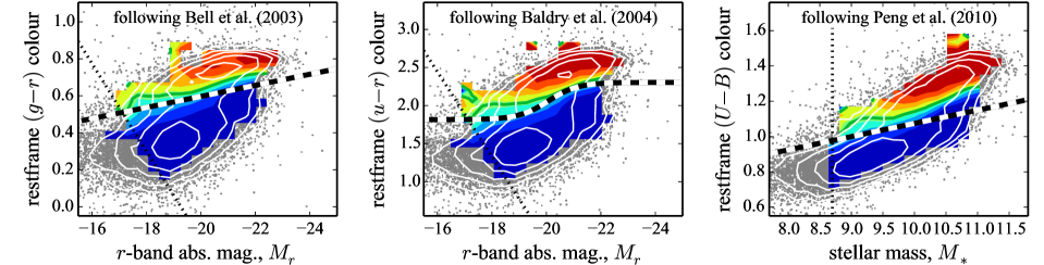
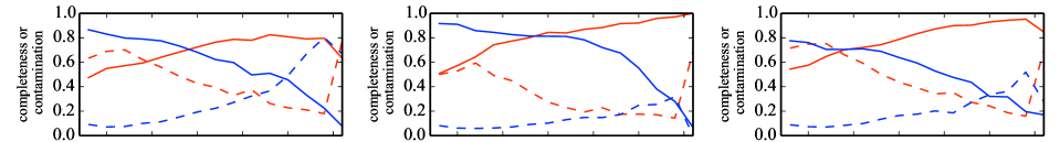
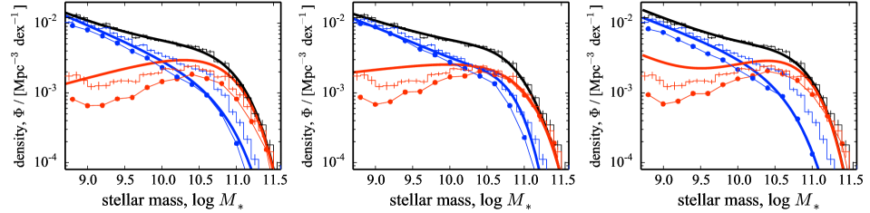
Figure 14: Comparisons between our (objective) B/R classifications and the (largely arbitary) blue/red selections used in previous studies, and how these differences lead to very different mass functions.— This Figure is described and discussed at length in §9.1. The message to take from this Figure is that it is not possible to extract a clean sample of B- or R-type galaxies using a hard cut in an optical colour–magnitude or colour–mass diagram. Using the three selections shown, any ‘red’ sample is typically ‘contaminated’ by B-type galaxies at the $\gtrsim 25$ % level; something like 1/3 to 1/2 of all B-type galaxies would be selected as ‘red’. Further, in connection with the results of Peng et al. (2010), we raise the possibility that the apparent upturn in their ‘red’ MF might be simply explained as an overly aggressive ‘red’ cut. More than half of all $\log M_{*}<9.5$ galaxies counted as ‘red’ by Peng et al. (2010) are members of the bluer ‘B-type’ galaxy population.

We have now derived phenomenological descriptions of the B and R populations (§7; Fig.s 8–13), and have used this information to develop an objective, quantitative B/R classification scheme (§7.2; Fig. 10 and Fig. 11). Our final task is to compare our results to the existing results introduced in §4. Our discussion is based on Fig. 14. The basic point that we are trying to elucidate with this Figure is how our B/R-type classifications compare to the hard blue/red selection cuts employed or advocated by Bell et al. (2003), Baldry et al. (2004), and Peng et al. (2010), and how these different operational definitions for ‘blue’ and ‘red’ lead to very different quantitative results and qualitative conclusions.

Let us begin with a general description of what is shown in the different panels. As in Fig. 3, the top panels reproduce the colour-magnitude and colour-mass diagrams used by these authors to define their blue and red samples. In these panels, the filled coloured contours show how the fraction of R-type galaxies (as inferred from our fits to the $(g^{*}\!-i^{*})$ CMD) varies across the different colour-magnitude and colour-mass diagrams. These values have been obtained by 1/$V_{\mathrm{max}}$-weighted averaging of the values of $W{}_{\mathrm{R}}{}_{,i}\equiv\mathcal{L}{}_{\mathrm{R}}{}_{,i}/\mathcal{L}{}_{i}$—that is, the objective B/R-type classifier defined and discussed in §7.2—in bins of colour and magnitude/mass. In essence, if we were to observe many galaxies with the same or similar colour and magnitude/mass, the contours thus show what fraction of these galaxies we would expect to be members of the R population. Each of these cuts falls slightly blueward of the point where the R-type fraction is 50 %, which is shown by the heavy green line.

Unsurprisingly, there is a rather broad range of colours where there is substantial overlap between the B- and R-populations ($0.2\lesssim W{}_{\mathrm{R}}\lesssim 0.8$) in each of these diagrams. As we alluded in §4.3, this means that the different ‘blue’ and ‘red’ samples selected/defined by these different hard cuts will comprise a mix of both R- and B-type galaxies, in different proportions. As a means of selecting R- and B-type galaxies, these red and blue samples will all be both incomplete and contaminated. Further, the relative proportions of R and B galaxies in each sample—i.e., the degree of completeness/contamination—will be a strong function of mass, and will be sensitive to the precise cut used.

This is quantified in the middle row of Fig. 14. We can define a kind of quasi-completeness, $\mathcal{C}{}_{\mathrm{red}}$, for each of the red selections by looking at the relative numbers of R-type galaxies that satisfy each of the different red selections. This is simply derived as $\mathcal{C}{}_{\mathrm{red}}=\sum(W{}_{\mathrm{R}}{}_{,i}/V_{\mathrm{max}}{}_{,i})/\sum(1/V_{\mathrm{max}}{}_{,i})$, where the sum is over all galaxies satisfying the red selection, and similarly for $\mathcal{C}{}_{\mathrm{blue}}$. (Note that here, we are using the subscripts ‘blue’ and ‘red’ to denote the hard-cut samples, as distinct from our overlapping ‘B’ and ‘R’ populations.) Similarly, we can define a quasi-reliability, $\mathcal{R}{}_{\mathrm{red}}$, for each red selection as $\mathcal{R}{}_{\mathrm{red}}=\sum(W{}_{\mathrm{B}}{}_{,i}/V_{\mathrm{max}}{}_{,i})/\sum(1/V_{\mathrm{max}}{}_{,i})$, and similarly for $\mathcal{R}{}_{\mathrm{blue}}$. The completeness of each of the three different red and blue selections, so defined, are shown as a function of mass by the solid lines in the middle panels. We also show the degree of contamination, ($1-\mathcal{R}$), as the dashed lines.

This same information is re-presented in a different form in the lower panels of Fig. 3, which also serves to illustrate and elucidate how these effects lead to qualitatively and quantitatively different determinations of the red and blue, or R- and B-type, MFs. In each panel, the histograms with errors show our determinations of the R- and B-type MFs, $\Phi{}_{\mathrm{R}}$ and $\Phi{}_{\mathrm{B}}$, reproduced from Fig. 13; these are the same in each panel. Then, the solid lines show the fit MFs, $\Phi{}_{\mathrm{red}}$ and $\Phi{}_{\mathrm{blue}}$, from each of Bell et al. (2003), Baldry et al. (2004), and Peng et al. (2010). Note that for the purposes of this Figure, we have renormalised the literature MFs to match the integrated number density for the GAMA sample, in order to focus on differences in the shapes of the B/R and the blue/red MFs.

In each panel of Fig. 3, the points show the absolute numbers of B- or R-type galaxies that are ‘correctly’ selected as being blue or red; in other words, these are the galaxies that we can all agree on. These values are equivalent to $(\mathcal{C}{}_{\mathrm{blue}}\,\Phi{}_{\mathrm{blue}})$ and $(\mathcal{C}{}_{\mathrm{red}}\,\Phi{}_{\mathrm{red}})$. The difference between the points and the histograms thus reflects the effect of ‘incompleteness’ in the blue/red samples selected using a hard cut. Similarly, the difference between the points and the curves show the impact of ‘contamination’ in the hard-cut samples.

Having now described the content of Fig. 14 in general terms, let us now turn to discussing the results of each of these three works in the context of our more sophisticated analysis.

9.1.1 Comparing our analysis to Bell et al. (2003)

Looking at the left panels of Fig. 3, it can be seen that our B MF agrees well with the blue MF from Bell et al. (2003) for $\log M_{*}\lesssim 9.8$. But this agreement is at least partly coincidental. At these masses, compared to our B-classifications, the Bell et al. (2003) blue cuts are 80–90 % complete, and 80–90 % reliable. The red cuts, on the other hand, are only 50-60 % complete, and only 40–60 % reliable. It turns out that these two effects offset one another: the extra 10-20 % of B-type galaxies that are counted as red almost exactly balances the 50 % of R-type galaxies that are missed. In the context of our results, Bell et al. (2003) thus get the ‘right’ answer for the $\log M_{*}\lesssim 9.8$ red/blue MFs, but not necessarily for the ‘right’ reasons: even where our MFs are similar, they are counting very different galaxies.

At higher masses, there are large discrepancies between our MFs and those of Bell et al. (2003). Many of what we call ‘B-type’ galaxies are counted by Bell et al. (2003) as being ‘red’: the quasi-completeness of the Bell et al. (2003) selection drops rather smoothly from $\sim$ 75 % at $\log M_{*}\sim 10$ to $\lesssim 50$ % for $\log M_{*}\gtrsim 11.3$. This means that, even though the red selection is $\gtrsim 85$ % reliable, it is also contaminated by B-type galaxies at the 20–30 % level. The obvious culprit here is dust, and specifically the dust-induced upturn in the $(g-i)$ CMR for the B population, as can be seen in Fig. 8 and Fig. 10.

The net effect of these effects is to inflate the red MF by a factor of $(\mathcal{C}{}_{\mathrm{red}}/\mathcal{R}{}_{\mathrm{red}})\sim 1.5$, and to depress the blue MF by a factor of $(\mathcal{C}{}_{\mathrm{blue}}/\mathcal{R}{}_{\mathrm{blue}})\lesssim 0.6$. In light of all this, the fact that the Bell et al. (2003) red/blue MFs can each be well described by a single Schechter function is somewhat coincidental.

9.1.2 Comparing our analysis to Baldry et al. (2004)

The Baldry et al. (2004) determinations of the red and blue MFs are based on similar assumptions to the ones that we have made. These authors have used an ad hoc iterative procedure to fit simultaneously for the centres of and scatters around the blue/red CMRs, as well as the MFs. Compared to our analysis, the major differences are: 1.) that their fits are to the $(u-r)$–$M_{r}$ colour–magnitude diagram, rather than the $(g^{*}\!-i^{*})$–$\log M_{*}$ CMD; 2.) that in their analysis, they bin the data first by magnitude, and then by colour, and fit to these binned distributions; and 3.) that they then rescale their values for each magnitude bin to stellar mass, using a simple relation between $(u-r)$ and $M_{*}/L_{r}$, whereas we are explicitly working with $M_{*}$ estimates from SPS modelling of optical SEDs.

Given the general similarities in, and important differences between, the two approaches, it is extremely encouraging that there is such good agreement between the B and R MFs that we derive, and those from Baldry et al. (2004)—at least at the high-mass end. There are still rather large differences between the red MF from Baldry et al. (2004) and the R MF that we derive from the $(g^{*}\!-i^{*})$ CMD, but we note that the results based on the $(g-i)$ CMD are in rather better agreement.

The cut shown in Fig. 14 has been derived by Baldry et al. (2004) on the basis of their fits. This cut is designed to maximise the product ($\mathcal{R}{}_{\mathrm{blue}}\mathcal{C}{}_{\mathrm{blue}}\mathcal{R}{}_{\mathrm{red}}\mathcal{C}{}_{\mathrm{red}}$) in $(u-r)$–$M_{r}$ space. In this sense, it is designed to be an optimal hard-cut blue/red selection line (given the specific tanh parameterisation used). From Fig. 14, it can be seen that this optimal selection is nevertheless imperfect. Using the Baldry et al. (2004) selection line, $\mathcal{C}{}_{\mathrm{red}}$ drops from $\sim 80$ % completeness at $\log M_{*}\sim 10$ to $\lesssim 65$ % for $\log M_{*}\gtrsim 10.8$; by the same token, $\mathcal{R}{}_{\mathrm{blue}}$ is $\lesssim 75$ % for all masses. (These numbers are entirely consistent with the caveats given by Baldry et al., 2004). This again serves to unambiguously demonstrate the difficultly of using a hard cut in an optical colour–magnitude or colour–mass diagram to meaningfully select red/blue galaxy samples.

9.1.3 Comparing our analysis to Peng et al. (2010)

Finally, let us turn our attention to the comparison between our results and those of Peng et al. (2010). This comparison is particularly interesting and important, given the elegant ‘semi-empirical’ model for the quenching of star formation within galaxies that these authors have advanced based on their results.

The Peng et al. (2010) model predicts a single Schechter function for star-forming galaxies, and a two-component Schechter function for quenched/passive galaxies. The model also makes the specific prediction that the secondary component of the MF for quenched galaxies should have the same shape as, but a lower normalisation than, the MF for star-forming galaxies. They show that their observed blue/red MFs, based on data from SDSS and zCOSMOS, and selected using the cut in the $(U-B)$-$M_{B}$ colour-magnitude diagram, can be understood in this way.

From Fig. 14, it is clear that the Peng et al. (2010) cut is rather bluer than others, such that their blue sample is only $\sim 80$ % complete for B-type galaxies, even at the lowest masses. In other words, fully $20$ % of what we classify as ‘B-type’ galaxies would be counted by Peng et al. (2010) as ‘red’. By the same token, their red sample is heavily contaminated: more than half of those galaxies selected as red/quenched by Peng et al. (2010) are classified by us as being B-type.

This is absolutely crucial in the context of the Peng et al. (2010) model, which makes the specific prediction that the secondary component of the MF for quenched galaxies should have the same shape as, but a lower normalisation than, the MF for star-forming galaxies. It should now be clear how exactly this kind of behaviour can be produced by using too-blue a cut: once the red-selected sample becomes highly contaminated, it becomes simply a shadow of the blue MF. This effect does not rely on, but will be amplified by, the effects of photometric scatter discussed in §4.1.

We thus highlight the possibility that the low mass upturn in the red MF seen by Peng et al. (2010) and others simply reflects a high degree of ‘contamination’ of the ‘red’ sample by members of the ‘blue’ population. This happens where the relative numbers of red galaxies is low, and the hard red/blue selection limit enters the red wings of the blue distribution. This interpretation also explains why the red upturn has a similar shape to the blue MF: because the galaxies responsible for this upturn are actually members of the blue population.

Taken at face value, our results would therefore appear to be in conflict with the quenching model advanced by Peng et al. (2010). However, this statement is only true to the extent that our R-type galaxies can be interpreted, in astrophysical terms, as being genuinely ‘quenched’. But still, looking at Fig. 14 and back to Fig. 7, the same criticism could be levelled at Peng et al. (2010).

In light of the above, the strongest point that we are prepared to advocate at this stage is only that the relative shapes and absolute values of the B and R (or blue and red) MFs depends very sensitively on how the different populations are defined/selected/classified (see also, e.g. Driver et al., 2006; Kelvin et al., 2014, among others). Further, we stress the dangers of over-interpretting the physical significance of any hard red/blue selection, given the basic fact of overlap between the two R and B populations. This is precisely why we have set out to derive objective and phenomenological B/R classifications, which are empirically derived from our statistical description of the observed data.

9.2 Comparisons with other approaches of distinguishing galaxies with ‘young’ and ‘old’ stellar populations

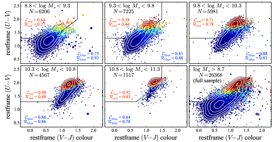
Figure 15: The optical-to-NIR SED shapes of B- and R-type galaxies.— Each panel shows the restframe UVJ colour-colour distributions of galaxies in different mass bins. In each panel, individual galaxies are colour-coded according to their B/R-type classification, as in Fig. 11. The white contours show the logarithmic data density. As would be expected if the R-type galaxies were mostly ‘red and dead’, they fall in a relatively tight clump. Further, the R-type clump is offset from the red tip of the B-type galaxy distribution. Note that the derivation of these restframe colours is entirely independent of the SED fits used to derive the values of $(g^{*}\!-i^{*})$, whence the B/R classifications. The situation of R-type galaxies in the ‘old’ part of the diagram (shown by the black box) is not by construction. While it is reassuring that these two complementary approaches qualitatively agree, in contrast to ‘hard’ colour selections, we stress that our B/R-classification scheme is objective (derived from the data, rather than imposed on it), and quantitative (explicitly accounting for overlap between two populations). In this context: consider how many B-type galaxies with $\log M_{*}<9.3$ would satisfy a UVJ ‘red’ selection, despite clearly being associated with the main blue clump. Also: consider how the mass function of these UVJ ‘red’ galaxies will behave at low masses.

The basic problem that we have sought to overcome in our analysis is that the optical colour distributions of the B and R populations overlap. We are certainly not the first to apprehend the difficulties in using optical colours to distinguish ‘developed’ from ‘developing’ galaxies. Our solution to this problem has been to devise a mixture modelling approach to account for this fact. Most authors, however, have sought to circumvent these problems, rather than attempt to confront them head on.

Many others have argued that an optical–NIR colour–colour diagram (see e.g., Labbé et al., 2006; Williams et al., 2009; Papovich et al., 2012) can be used to isolate ‘quiescent’ galaxies. The idea is that the dust and age/metallicity vectors are no longer parallel in a such a diagram, and so ‘red and dead’ galaxies and ‘dusty star-formers’ are more easily separated. This kind of colour selection thus acts as a very simple (two-colour) SED-based classification.

Taking this idea to its logical conclusion, other authors have explicitly used SPS modelling of SEDs to develop a young/old classification scheme. For example, Drory et al. (2009) have selected ‘passive’ galaxies based on the best-fit SPS template. After the fact, they then show that these ‘passive’ galaxies are indeed concentrated in the expected region of the NUV–$r$–$J$ colour–colour diagram.

By considering the intrinsic stellar $(g^{*}\!-i^{*})$ color, we have used the information encoded in the multicolour SEDs to, insofar as is possible, break the degeneracy between dust and age/metallicity. In this way, we are using $(g^{*}\!-i^{*})$ as a continuous and quantitative diagnostic of a galaxy’s stellar population. Then, we have used a phenomenological, descriptive model of the bivariate $M_{*}$–$(g^{*}\!-i^{*})$ distribution to derive a quantitative, probabilistic classification scheme. Next, similar to Drory et al. (2009), we can elucidate the nature of—and validate our interpretation of—these classifications by showing how our classifications map onto other common diagnostic plots.

9.2.1 The optical–to–NIR colours of B- and R-type galaxies

We explicitly show how our B/R-classification scheme maps onto the UVJ diagram in Fig. 15, which shows the galaxies in our sample, separated into broad mass bins, and colour-coded according to their objective B/R-type classification, $W{}_{\mathrm{R}}$. These plots can be compared to the restframe UVJ colour–colour diagram used by, for example, Williams et al. (2009) to and isolate the ‘dead sequence’ of truly passive galaxies at high redshifts.

For this Figure, the restframe UVJ photometry have been derived using a heavily refactored version of the InterRest algorithm for interpolating restframe photometry (Rudnick et al., 2003; Taylor et al., 2009). It is worth stressing that the derivation of these restframe colours is completely independent from the SED fits used to derive the values of $M_{*}$, $(g-i)$, $(g^{*}\!-i^{*})$, etc.

It can be seen that, in broad terms, our $(g^{*}\!-i^{*})$-based separation between B- and R-type galaxies behaves as expected in the UVJ colour–colour diagram: the R-type galaxies are tightly clustered, and in a location that is above and/or to the left of the ‘blue sequence’. This demonstrates that our optical SED fits can distinguish between the SEDs of ‘red and dead’ galaxies and ‘dusty star formers’, and thus that our values of $(g^{*}\!-i^{*})$ do provide a meaningful characterisation of galaxies’ stellar populations.

The different panels Fig. 15 show how our B/R-type classifications is projected onto the UVJ diagram at different mass ranges. Looking at the classifications, the point of transition from mostly B-type (blue points) to mostly R-type (red points) can be seen to correspond qualitative changes in the 2D data density that, in simple terms, look like different populations.

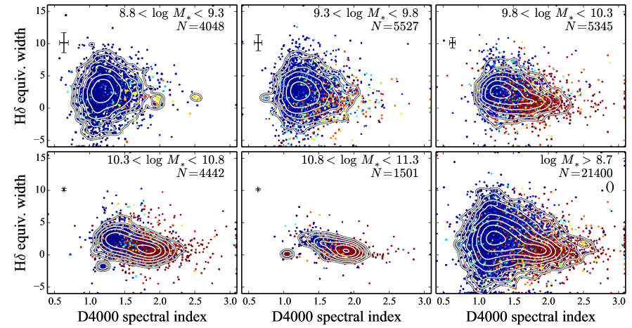
Figure 16: The optical spectral shapes of B- and R-type galaxies.— Each panel shows the bivariate distribution of 4000 Å break strength, parameterised by the $D_{4000}$ diagnostic, and the equivalent width of the H$\delta$ line (positive implies emission). As in Fig. 15, each panel is for a different mass range, and individual points are colour-coded according to $W_{R}$. A spectral signal-to-noise cut has been imposed to ensure meaningful measurements of both $D_{4000}$ and H$\delta$. As for the previous Figure, these diagnostic plots show how our B/R classifications do meaningfully encapsulate information about differences in galaxies’ stellar populations. Further, as in Fig. 15, the B/R classifications can be seen to correspond to differences in SED shape that can be broadly understood in terms of younger/older stellar populations. More specifically, that the light from R-type galaxies is completely dominated by stars with ages $\gtrsim 1$ Gyr.

It can be seen in this Figure that there is some mass-dependent ‘creep’ to how our B/R classification maps onto the UVJ diagram. From a phenomenological point of view, however, the argument could be made that this is desirable. Certainly, it is clear that the locus of ‘red’ galaxies, however defined, shifts to redder colours at higher masses. This is just the colour–mass relation in another guise. Indeed, in the lower mass bins our B/R-type classifications might provide a better characterisation of the two-population nature of the data than the standard hard selection box shown.

It is worth explicitly noting that the UVJ selection box shown would capture predominately B-type galaxies at the lowest masses: the ‘reliability’ of a UVJ selected sample of R-type galaxies would be only $\sim 25$ %. In comparison to our determination of the R MF, such a UVJ-selected ‘red’ MF would be inflated. Moreover, this would act in such a way that the inferred ‘red’ MF would have approximately the same low mass slope as the ‘blue’ one. This is highly significant in the context of the results of Peng et al. (2010).

9.2.2 R-type galaxies have older stellar populations

Fig. 16 shows a similar but different test, this time using the $D_{4000}$ and H$\delta$ spectral diagnostics. These measurements have been made using the available GAMA or literature spectra for each galaxy in our sample. For the purposes of this plot, we have imposed a signal-to-noise cut across the relevant wavelength range to ensure reasonable data quality. This effectively introduces a bias against the reddest galaxies, particularly at low masses. Representative error bars for each bin are shown.

In this diagram, stars with ages $\gtrsim 1$ Gyr will have both $D_{4000}\gtrsim 1.5$ and H$\delta\lesssim 0$ (see, e.g. Kauffmann et al., 2003, among many others). Because these measurements are made over a narrow wavelength range, they are very weakly sensitive to dust. This diagnostic diagram shows that the optical spectra of R type galaxies are completely dominated by old stars, with little to no contribution from stars less than $\sim 1$ Gyr old. In other words, and modulo the caveat in the previous paragraph, these results suggest that those galaxies that we have classified as R-type have seen no significant star formation activity in the past 1 Gyr or more.

The results presented in this section are intended to demonstrate two important facts. First, the results shown in each of these two figures illustrate that—and how—our B-R classifications faithfully and meaningfully encapsulate differences in galaxies’ SED shapes, and hence stellar populations. In particular, these Figures show how, particularly for $\log M_{*}\gtrsim 10$, the R-type population is analogous to commonly used ‘red and dead’, ‘passive’, or ‘quenched’ selection criteria.

Second, and more perhaps more importantly, we have presented these diagnostic diagrams as a means to evaluate the meaning of our phenomenological and empirically derived B/R classification scheme. Earlier, in §4, we have said that our results can be used to gain insight into the process of quenching, but only to the extent that our operational definitions of ‘red’ or ‘R’-ness can be taken to mean ‘quenched’. In this regard, we can now offer a more astrophysical characterisation of what distinguishes R- and B-type galaxies: namely, that the light from R-type galaxies is completely dominated by stars with ages $\gtrsim 1$ Gyr.

9.2.3 Understanding the nature of B- and R-type galaxies

In this work, we have used the intrinsic, dust-corrected $(g^{*}\!-i^{*})$ colour as a diagnostic parameter for a galaxy’s stellar population. As mentioned in §2.3.2, this quantity is a very good proxy for luminosity-weighted mean stellar age. We have then used our parametric, descriptive mixture-modelling of the $(g^{*}\!-i^{*})$ CMD to construct an objective B/R-type classification scheme, and so derive operational definitions for these designations. In this section, we have used complementary diagnostics to show that the stellar populations of B- and R-type galaxies do indeed differ, and in particular that R-type galaxies really do host older stars. This demonstrates that the $(g^{*}\!-i^{*})$ parameter is indeed a useful diagnostic for distinguishing galaxies based on their stellar populations.

The line of argument that we have now developed is similar to the one in Drory et al. (2009). In particular, we have now explicitly demonstrated, in a mass dependent way, that galaxies classified as R-type or B-type have different spectral and SED shapes, and thus that the two populations have qualitatively different stellar populations. (We also show how the kind of UVJ cuts commonly used can give very misleading results at low masses.)

The crucial point of difference between our analysis and those mentioned above is this: we have not explicitly set out to distinguish ‘young’ and ‘old’ (or ‘star forming’ and ‘quenched’) stellar populations. Instead, we have started from a phenomenological description of the optical colour–mass diagram, and used this to disentangle the two apparently distinct populations. Identifying the distinguishing features of galaxies in these two populations is thus, for us, a secondary problem. In this sense, the implication from Fig. 15 and Fig. 16 is that massive R-type galaxies have relatively old stellar populations, and little to no dust. This point is non-trivial, even if it may seem so at first blush.

9.3 Fallacious arguments against our methods and results

9.3.1 40 parameters is too many. Therefore I do not believe your results.

In §5.3, we have described the various tests that we have done in an attempt to devise the best and simplest description of the data possible. This is not to say, however, that our parameterisation is right. Instead, our claim is only that we do provide a good description of the data, inasmuch as our model encapsulates all the qualitative features of the bivariate colour–mass distributions, as illustrated in Fig.s 6–13.

There are some indications that some parameters could be eliminated from the model without significantly degrading the statistical quality of the fit: most notably, the data do not clearly demand a two-Schechter description of the R MF. While there is some ambiguity in whether or not certain parameters ought be excluded or included, we can say with confidence that we are not grossly overfitting the data.

There are some parameters for which the inferred values are consistent with zero (see Fig. 5). To the extent that the model does not make use of the additional freedoms that these parameters allow, they would appear unnecessary for the best, simplest possible description of the data. At the same time, and for the same reason, excluding these parameters would make no difference to the fits, or to our results. To the extent that the decision as to whether or not to include these parameters is arbitrary, it is also unimportant.

9.3.2 Your results are entirely determined by how you have parameterised your model. Therefore I do not believe your results.

As discussed in §5.3.2, this same criticism could be levelled at any model or modeller. The decision as to how to model one’s results is an inescapable part of any modelling.

Furthermore, in the specific context of modelling the bimodality in the CMD, this concern is misplaced. As discussed in §4 and §9.1, the use of a hard cut to select ‘red sequence’ and ‘blue cloud’ galaxies directly determines the inferred shapes of the mass functions. And as discussed in §4.3, in the absence of some solid theoretical justification for the specific cuts used, these cuts must be viewed as being to some extent arbitrary. This criticism is thus much more pertinent for the vast majority of existing bimodality studies (the notable exception being Baldry et al., 2004).

Indeed, as laid out in §4, the motivation for our analysis is precisely to address this concern, insofar as is possible. Our primary motivation for our mixture model of the bivariate colour-mass distributions is to develop an objective classification scheme, which can be used to disentangle the apparently distinct populations.

But this is not to deny the truth that the form of the model influences the outcome. Indeed, as discussed in §6.2, this idea leads to an important caveat on our MF determinations for $\log M_{*}\lesssim 9.3$, where the application of our model to the observed colour distributions becomes problematic (see Fig. 6 and Fig. 7).

9.3.3 You cannot place strong constraints on the value of parameter $X$, and anyway, all of your parameters are strongly covariant, if not completely degenerate. Therefore I do not believe your results.

By using a Bayesian MCMC sampling scheme to constrain the values of the parameters in our model—i.e., to do the actual fitting—we fully determine and account for the covariances between the model parameters. Further, as discussed in §7.3, we are not specifically interested in the actual values of most of the parameters that define the model. For example, the values of the parameters $\alpha_{\mathrm{B},2}$ and $M^{\dagger}_{\mathrm{B},2}$ are important only insofar as they describe the shape of the MF for the B population. As shown in Fig. 12 and Fig. 13, we do not need to be able to uniquely determine the values of the $\alpha$s or $\phi^{\dagger}$s in order to obtain very precise determinations of the MF.

As discussed in §7.3, ‘the results’ of our analysis should be taken to be the histograms shown in Fig. 12 and Fig. 13. In deriving these results, the role of our parameterised model is only to provide objective and quantitative B- and R-type classifications, as discussed in §7.2, which account for the overlap between the two populations in the CMDs. As discussed in §7.3, uncertainties in the values of the different model parameters, propagated through to uncertainties in the classifications, produce uncertainties in our MFs that are at most $\sim 10$ %, and are more typically 1–5 %. For any given mass in either Fig. 12 or Fig. 13, the contribution to the total error budget associated with the construction of the model is always $\lesssim 40$ %, and more typically $\lesssim 10$ %.

9.3.4 It makes no sense to say that some ‘red’ galaxies are bluer than many ‘blue’ galaxies. Therefore your results are meaningless.

As discussed in §4.4, our analysis is predicated on two assumptions, neither of which are controversial, First, we are assuming that there are two populations, which are characterised/distinguished by their own distinct CMRs. Second, we are assuming that there is some scatter around these relations, to the point where the two populations are observed to overlap. Taken together, these two assumptions lead to the situation where, in principle and in practice, the bluest R-type galaxies may have bluer stellar colours than the reddest B-type galaxies. This is precisely the reason why we choose to refer to the populations using the more neutral designations ‘B’ and ‘R’: to try to avoid some of the confusion that comes from the strong connotations that have come to be associated with these words. Some care is therefore required in interpreting our results in astrophysical terms (see the caveats given in §8).

Furthermore, we stress that previous results that have used a hard cut overlook the empirical fact of scatter in the colour distributions for the ‘blue’ and ‘red’ populations. Some care is also required in interpreting the results of past bimodality studies in astrophysical terms. We would therefore invert this criticism to argue that past studies have selected the red tail of the B population—galaxies that have young, blue stellar populations—and called these galaxies ‘quenched’ (see Fig. 14 and in particular Fig. 15).

9.3.5 Your so-called model contains no physics, and therefore no information about the process of galaxy formation.

Again, we make no pretence that our particular parameterisation is in any way physically meaningful; only that it yields a good description of the phenomenology of the CMD. Our results thus offer one potential means of understanding the data, which is the most that any modeller can do. Included within this is a phenomenological description of how the general population can be decomposed into two distinct but overlapping populations. Our hope here is that our empirical results can be used to guide and inform the future development of genuine semi-analytical and SPH models of galaxy formation in a cosmological context.

What we have done in this work is to develop a means for objectively and quantitatively classifying galaxies according to their stellar populations. In the broader context of this series of papers, our ultimate goal is to use these classifications to identify the physical differences between B- and R-type galaxies, with a view to deriving empirical constraints on the physical processes that act to determine whether any particular galaxy is B- or R-type. We therefore defer more astrophysically-minded observational studies of the galaxy bimodality (or bimodalities?) to future works.

9.3.6 Your R-type galaxies do not conform to existing notions of ‘red and dead’ or ‘quenched’, and therefore your results tell me nothing about the different stellar populations and/or star formation histories of ‘developed’ and ‘developing’ galaxies.

In the first instance, our goal has been to separate the general galaxy population into two subpopulations, on the basis of their constituent stellar populations, and in a mass dependent way. For our analysis of the effective $(g-i)$ CMD, dust is a confounding factor. For this reason, we have repeated our analysis looking at intrinsic, dust corrected $(g^{*}\!-i^{*})$ colours.

It is true that degeneracies between dust, metallicity, and SFH in such fits mean that the uncertainties in the values of $A_{V}$, $Z$, or $\tau$ can be large, but we maintain that these data are sufficient to make the qualitative distinction between dusty and old SED shapes. In support of this claim, we have shown in §9.2 that those galaxies that we classify as being either B- or R-type occupy different regions of the H$\delta$-D₄₀₀₀ spectral line diagnostic diagram (Fig. 16), as well as the restframe UVJ colour-colour diagram (Fig. 15).

In other words, the B-/R-type classifications really do encapsulate meaningful information about galaxies’ stellar populations. Further, these classifications closely correspond to the two-population distributions seen in both diagnostic plots. Conversely, we have also argued the kinds of ‘red’ selections that are commonly used are a poor proxy for ‘quenched’.

We have thus accomplished our primary goal of disentangling and characterising the two apparently distinct populations seen in the CMD. Some of our R-type galaxies conform to the usual picture of ‘red and dead’ galaxies, but we have shown that these galaxies are just the high mass tip of a more continuous R population.

With our primary goal accomplished, our phenomenological characterisations of these two populations can then shed light on their astrophysical nature. This includes the MF for each population, which now represents a target for cosmological simulations to aim at. This also includes our characterisations of the $(g^{*}\!-i^{*})$ and $(g-i)$ CMRs for each population, which provide qualitative constraints on the processes of star formation and of star formation quenching within galaxies.

9.3.7 Galaxies are complicated, and focussing on only two or three parameters glosses over all the important details. You are missing the trees for the forest.

The process of galaxy formation is complicated, and there are myriad well-known and studied galaxy types and classes that we have not considered in our analysis: e.g., radio loud AGN, starbursts, E+A or post-starburst galaxies, satellites/centrals, interacting and merging galaxies, etc. Some or all of these processes may play an important role in determining whether a particular galaxy is R-type or B-type, or conversely, some of these processes may act exclusively on or within R- or B-type galaxies. In this way, these processes are presumably also responsible for producing the observed intrinsic scatter around each of the two CMRs.

By the same token, galaxies are in general multi-component systems. As a simple example, most massive galaxies have both a disk and a bulge component, with separate stellar populations and formation mechanisms. For example, Driver et al. (2006) have argued that galaxies’ global colours are driven by the mixture of (blue) disk stars and (red) bulge stars, and that the colour bimodality is thus best understood in terms of the (bimodal) distribution of bulge-to-disk mass ratios.

We have deliberately avoided these kinds of questions in this work; our intention is only to derive an empirical, phenomenological description of the apparent dichotomy in the stellar populations of field galaxies—that is, the nature of the R- and B galaxy populations. In doing so, we have derived an objective, operational definition for these designations. This is a necessary prerequisite for future studies of the different astrophysical natures of these two galaxy populations, which we will pursue in future papers.

In light of the above, it is remarkable that this game can be played at all. Here again, we stress there are no clear signs of an intermediate or transition ‘green’ population. That the bivariate colour–mass distribution for the field galaxy population is extremely well described by a simple two-population model implies that our phenomenological distinction between B- and R-type galaxies does indeed encapsulate some important astrophysical differences in the formation histories or evolutionary states of these two populations—even if we cannot yet articulate what these differences are, or what the driver for these differences may be.

10 Summary and Conclusions

Our particular interest lies in characterising the mass functions (MFs) and colour-mass relations (CMRs) for the apparently distinct populations seen in the optical colour-mass diagram (CMD), where the two populations are distinguished on the basis of galaxies’ stellar populations. Our analysis is based on a sample of $\log M_{*}>8.7$ and $z<0.12$ field galaxies from the Galaxy And Mass Assembly (GAMA) survey. This sample is properly mass-complete (volume limited) for $\log M_{*}\gtrsim 10$; for lower masses, we have used the standard $1/V_{\mathrm{max}}$ formalism to account for incompleteness (see §3). Note that none of our results or conclusions change if we limit our analysis to $\log M_{*}>9.5$, or to $z<0.06$.

The immediate motivation for reconsidering this well-studied problem is that, as discussed in §4.3, there are quantitative and qualitative disagreements between the MF determinations that exist in the literature. First, we have shown that if we analyse our GAMA-sample in the same way as each of Bell et al. (2003), Baldry et al. (2004), and Peng et al. (2010), we are able to reproduce each of these authors’ SDSS-based results. Then, we argue that the discrepancies between the results and conclusions of these studies are due entirely to the different (and most often arbitrary) ways that the ‘blue’ and ‘red’ galaxy samples have been selected/defined.

Our first and most important conclusion is therefore a qualitative one: that the largest uncertainty in previous characterisations of the mass functions for ‘red’ and ‘blue’ galaxies is tied to how these terms are defined. Put bluntly, the main reason why, say, Peng et al. (2010) see an upturn at the low end of the ‘red’ MF where, say, Bell et al. (2003) do not is simply because the Peng et al. (2010) definition of ‘red’ is considerably bluer than the Bell et al. (2003) one. As a direct consequence, a significant fraction of the Peng et al. (2010) ‘red’ sample are star forming galaxies with young stellar populations (see Fig.s 4, 14, and 15).

The direct implication is that the power of these results to provide useful constraints on the process of galaxy evolution is directly limited by the extent to which the specific ‘red’ and ‘blue’ selections used can be shown to be astrophysically meaningful. In the absence of convincing arguments in favour of any one of these selections over the others, important questions like the mass range over which the galaxy population transitions from mostly blue to mostly red, or the low mass slopes of the blue and red mass functions, are left largely unconstrained. In order to address these questions, what is needed is a well-motivated operational definition for the technical terms ‘red’ and ‘blue’.

To redress this, we have developed a descriptive model for the distribution of galaxies in CMD, with the specific goal of distinguishing between ‘developed’ and ‘developing’ galaxies on the basis of their stellar populations. In our modelling, we treat the observed data distribution as being the sum of two distinct but overlapping populations. The model also includes a ‘bad’ component to allow for outliers, catastrophic errors, or otherwise un- or under-modelled aspects of the observed distributions (see §5.1.4 and §7.1). The formalism for our modelling, which is developed pedagogically in Appendix A, is based on the method of (Gaussian) mixture modelling (see, e.g., Hogg, Bovy & Lang, 2010).

As outlined in §5.1, in its most general form, our descriptive model is fully defined by 40 parameters. As discussed in §5.3, not all of these parameters are strictly necessary for a ‘good’ description of the data. In particular, it is not clear that the data strictly demand a second Schechter component to well describe the MF for the R population. As discussed in §5.3.2, however, where there is ambiguity about whether or not a parameter is necessary, it will have little to no impact on the final results. Beyond that, the most that we can say is that we have made every attempt to ensure that we are not grossly overfitting our data.

In effect, there are two assumptions that underpin our approach. First, we are assuming that some physical process(es) or hidden parameter(s) act to determine whether a given galaxy is a member of one or the other population; that is, we assume that there are two populations, which follow distinct CMRs. Then, some secondary process(es) or parameter(s) determines where that galaxy falls with respect to the main CMR for that population; that is, we assume that there is some (Gaussian) scatter around each of the two CMRs, to the point that the two populations are observed to overlap in an optical CMD (or, indeed, in a UVJ colour–colour diagram). Neither of these assumptions ought to be controversial.

Allowing that, at fixed mass, there is some overlap between the ‘blue’ and ‘red’ colour distributions inescapably implies that some ‘red’ galaxies will have bluer colours than some ‘blue’ galaxies. In acknowledgement of this semantic trap, and to avoid some of the confusing connotations associated with the terms ‘blue’ and ‘red’, we have adopted the more generic designations of ‘B’ and ‘R’ to describe the two populations seen in the CMD (see §4 and §6.1).

That is, rather than considering blue and red galaxies, we focus on two galaxy populations, which we dub B and R. It is not necessarily true that a particular B- galaxy will be bluer than some other R-galaxy. It is also not necessarily true that an R-type galaxy can be thought of as being ‘red and dead’, ‘early type’, ‘quiescent’, etc. It nevertheless remains true that the distribution of stellar population properties are different for galaxies in each of the two populations—in particular, at fixed mass, and on average, galaxies in the B-population have bluer (and so younger) stellar populations than those in the R-population.

In other words, we are assuming that the phenomenological separation of the general galaxy population into B- and R-type subpopulations somehow reflects a qualitative binarity in the formation histories or evolutionary states of galaxies—but it remains to describe and explain precisely how and why this is the case. By modelling these populations, we can actually derive from the data phenomenological working definitions for the terms ‘B-’ and ‘R-type’ (see §7.2, Fig. 10, and Fig. 11). What is more, the classifications are objective, insofar as objectivity is possible (see §5.3.2).

Bearing in mind the caveats given above, we go on to describe the basic characteristics of the B- and R-population in terms of both the effective $(g-i)$ CMD (Fig. 8), as well as the intrinsic, dust-corrected colour, $(g^{*}\!-i^{*})$ CMD (Fig. 9). That the members of these two populations comprise genuinely different stellar populations has been demonstrated in §9.2, where we show that R- and B-type galaxies occupy distinct regions of the UVJ and $D_{4000}$–H$\delta$ diagnostic diagrams (Fig. 15 and Fig. 16).

We find that the intrinsic $(g^{*}\!-i^{*})$ CMR for the B population is both considerably tighter and more linear than the effective $(g-i)$ CMR. This implies that the both the upturn in the $(g-i)$ CMR at $\log M_{*}\sim 9.5$ and the relatively large scatter around the $(g-i)$ CMR at all masses is driven by the distribution of dust properties, rather than differences in the stellar populations of these galaxies. At least for $\log M_{*}\lesssim 10.8$, the relative flatness of the $(g^{*}\!-i^{*})$ CMR for B-type galaxies also implies that, in terms of stellar colours, the B population is relatively homogenous.

This behaviour changes, however, for $\log M_{*}\gtrsim 10.8$. At this mass range, the B population appears to converge with the red sequence in the $(g-i)$ CMD. This is also where the MF for B galaxies drops off very rapidly. In other words, there are few if any galaxies with $\log M_{*}\gtrsim 10.8$ with young (B-type) stellar populations; this represents the top end of the blue sequence.

For the R population, if nothing else, we can say with confidence that there are essentially no $\log M_{*}\lesssim 9$ field galaxies with stellar populations that are the same as or similar to those of the genuinely ‘red and dead’ galaxies seen at the highest masses. Instead, at least for $\log M_{*}\gtrsim 9.8$, we see a gradual trend whereby less massive galaxies have progressively bluer stellar colours (i.e., younger luminosity-weighted mean stellar ages and/or lower mean stellar metallicities) than their more massive cousins.

The relatively small dispersion in $(g^{*}\!-i^{*})$ CMR for the R-population suggests that, at fixed mass, R-type galaxies have rather similar stellar populations, and hence similar star formation/stellar assembly histories. At the same time, the slope of the $(g^{*}\!-i^{*})$ CMR for R-type galaxies shows that there are differences in the evolutionary histories of different members of the R populations with different present day masses. Said another way, the evolution of individual R-type galaxies in the field proceeds in such a way as to create or preserve the correlation between the stellar mass on the one hand, and stellar population on the other.

These observations—the relative homogeneity of the stellar colours of B-type galaxies, and the correlation between stellar mass and stellar population for R-type galaxies—run counter to prevalent notions of the ‘red sequence’ and the ‘blue cloud’. They also provide meaningful targets for theoretical models of galaxy formation and evolution to aim for.

For $\log M_{*}\lesssim 9.5$, it becomes increasingly difficult to meaningfully and robustly distinguish two separate B and R populations from the joint $(g-i)$ and $(g^{*}\!-i^{*})$ colour-mass distributions. Indeed, looking only at the observed colour distributions in bins of mass (Fig. 6 and Fig. 7), there is little to no clear evidence for a distinct R population at $\log M_{*}\lesssim 9$.

Our claim is therefore that, below $\log M*\sim 9.3$, we are no longer able to unambiguously identify a distinct R-component to the general field population: at least for field galaxies, below $\log M_{*}\sim 9.3$, the R population dissolves into obscurity. At these low masses, our characterisation of the R population may be better interpreted as describing the degree of asymmetry in the observed colour distributions, and our MF for the R population may be taken as an upper limit on the number of galaxies that lie outside the main colour distribution for ‘normal’ B-type galaxies (see §6.2).

We note in passing that the data do not clearly demand an intermediate ‘green’ population: the data are very well described by a two-population model (see Fig. 6 and Fig. 7). Taking this remarkable observation at face value, this might imply that movement between populations is quick (see, e.g., Bell et al., 2004b). Alternatively, it could imply that movement within a population (for example, by satellite accretion/minor mergers) is much faster than movement between populations: a galaxy may be ‘passed’ from one population to the other, and then have its colour rapidly re-randomised according to the ‘normal’ colour distribution for its new population.

We also note that optically-identified AGN reside exclusively within the blue sequence defined by the B population (Fig. 1). That is, in terms of their stellar populations, AGN hosts do not clearly differ from ‘ordinary’ star forming galaxies. Certainly they do not represent a transition population that is intermediate between the B and R populations.

The MFs that we derive for the R and B populations are rather different to those for ‘red’ and ‘blue’ galaxies presented by other authors (see Fig. 14). The reasons for these differences are discussed first in §4.1, and then again in close detail in §9.1.

In particular, we find considerably more ‘B’ galaxies with $\log M_{*}\gtrsim 10$, and a much more abrupt drop-off in the B MF at $\log M_{*}\gtrsim 10.8$. Whereas others put the crossover mass, where the two MFs intersect, at $\log M_{*}\approx 10.0$–10.3, we find it to be closer to 10.5. Further, our MF for R-type galaxies is also considerably lower at low masses than those for ‘red’ galaxies from the literature. If these red or R-type MFs can be used to probe the process of quenching, our results would imply that quenching is less prevalent—or equivalently, that massive galaxies continue forming new stars for longer—than has been previously thought.

But this leads to the final and most important caveat: as discussed at length in §4 and §6.1, there is real danger in inappropriately reifying the terms ‘B-’ and ‘R-type’—or, equally, the terms ‘blue’ or ‘red’. These terms must be understood as qualitative, phenomenological designations for galaxy populations. In particular, one should not conflate the terms ‘R’ or ‘red’ with the term ‘quenched’. This is especially true at low masses, where the stellar populations of ‘red’ or R-type galaxies are rather different to those found at higher masses.

As discussed throughout this paper, it is necessarily and inescapably true that our results depend on the choices made in the construction of our model—we can only answer the question that we have asked. In particular, the decision to use Gaussians to describe the colour distributions at fixed mass is primarily one of convenience. Our justification for these decisions is ultimately empirical—the proof is in the pudding. We have thus shown that our descriptive modelling provides one potential way of understanding the data. The fact nevertheless remains that using a different operational definition for the terms ‘red’ and ‘blue’ will lead to quantitatively and perhaps qualitatively different results.

We do not pretend to be immune to these difficulties. Instead, our goal is to highlight the importance of these issues, and to make it clear that the same criticisms can and should be levelled at any study of the ‘red’ and ‘blue’ galaxy populations. But then again, we have also validated our results by showing how the phenomenological B/R classifications that come from our model do indeed select galaxies with qualitatively different stellar populations.

This point is particularly significant in connection with the elegant semi-empirical model for quenching presented by Peng et al. (2010), which hinges on the presence or absence of an upturn to the MF for quenched galaxies at $\log M_{*}\lesssim 9.5$. Looking at the distributions shown in Fig. 6 or Fig. 7, (or even the UVJ diagrams in Fig. 15) it should be immediately obvious how problematic it is to meaningfully distinguish a separate ‘red’ or ‘quenched’ or even ‘R’-type population at these low masses (see §6.2). Further, it must be recognised how a sample of ‘old’ or ‘quenched’ galaxies selected using a hard cut in any of these diagrams—including the UVJ diagram—will be dominated at low masses by spillover from the red tail of the distribution of otherwise normal, young, star-forming, B-type galaxies. The critical issue is therefore whether or in what sense these galaxies can be thought of as a distinct, coherent population of quenched galaxies.

This paper is the first in a series in which we explore the different aspects or manifestations of the bimodality (or bimodalities) in galaxy properties. In Papers II and III, we will perform a similar analysis to explore bimodalities in terms of line emission properties, and in terms of Sérsic-fit structural parameters. Taken together, these three Papers will provide a basis for robustly and objectively classifying galaxies according to the stellar populations, present day star formation and/or AGN activity, and structure. In future works, we will go on to use these results to explore the natures of, and interrelations between, these bimodalities.

Appendix A Developing an Objective Red/Blue Classification Scheme

A.1 Introductory Statement of the Problem

Our overarching goal is to derive an empirical, phenomenological description of the ‘bimodality’ in the galaxy population, as seen in the $(g-i)$ and $(g^{*}\!-i^{*})$ CMDs. This apparently simple project is made problematic by the fact that the apparently distinct ‘red’ and ‘blue’ populations are seen to overlap in both of these CMDs. Accordingly, we want to avoid imposing some arbitrary ‘hard’ cut to distinguish ‘red’ from ‘blue’; instead, we want to develop the means to simultaneously and flexibly describing these two distinct but overlapping populations. The solution to this modelling problem—the method of mixture modelling—can alternatively be viewed as the development of an empirical and objective ‘red’/‘blue’ classification scheme, based on the likelihood that a given data point has been drawn from one or the other population.

To reduce the problem to the simplest possible terms, what we want to do is to construct a parametric model that describes the distribution of data points in the CMDs. This model will need to have two components—one for each of the ‘red’ and ‘blue’ populations—each of the form $p(x,~{}y)$, where $x=\log M_{*}$ and $y=(g-i)$ or $(g^{*}\!-i^{*})$. The model itself will be fully described by a set of parameters, $\mathbf{P}$. The observed data are then considered as having been randomly drawn from—generated by—this modelled density distribution, and observed subject to the appropriate measurement errors or uncertainties.

The generative model is thus explicitly intended to describe the (scalar) likelihood, $\mathcal{L}{}_{i}$, of observing any given (vector) datapoint, $\underline{x}{}_{i}=(x_{i},y_{i})$, and the associated uncertainties, which are assumed to be Gaussian, and are for now generically represented as $\sigma_{i}$. It is crucial to recognise that the generative model is only calculable—indeed, is only defined—given or assuming a particular set of trial values for each and every of the parameters in $\mathbf{P}$. That is, $\mathcal{L}{}_{i}$ describes the likelihood of observing the datapoint $\underline{x}{}_{i}$ with formal observational uncertainties $\sigma_{i}$, given or assuming a specific set of values for $\mathbf{P}$. To reflect this fact, the likelihood function is represented as $\mathcal{L}{}_{i}(\underline{x}{}_{i},\sigma{}_{i}|\mathbf{P})$.

The primary goal is thus to use the full observed dataset, $\mathbf{X}=\{\underline{x}{}_{i}\}$, along with the associated set of observational uncertainties, $\mathbf{S}=\{\sigma{}_{i}\}$, to constrain the ‘true’ values of the parameters in $\mathbf{P}$—that is, we aim to generate the posterior probability distribution function (PDF) for the values of the parameters $\mathbf{P}$, given that we have observed our data, $\mathrm{Pr}(\mathbf{P}|\mathbf{X},\mathbf{S})$.

Let us begin our discussion by considering only one population, and taking the simplest possible relation between $x$ and $y$: a perfect line, $\ell(\underline{x}|m,c)\equiv(m~{}x+c-y)=0$. In this case, the model parameter set $\mathbf{P}$ just comprises the slope and normalisation of the line; i.e., $\mathbf{P}=\{m,c\}$.

The traditional—but overly simple and somewhat naïve—approach to this kind of fitting problem is to use the method of weighted $\chi^{2}$ minimisation, which is described immediately below, to fit independently fit for a linear relation between $y$ and $x$. Among extragalactic astronomers, this approach is also frequently referred to as ‘maximum likelihood’. However, as is well known and accepted in many other disciplines (including particle physics and cosmology), and as we shall endeavour to make clear in the next few sections, the weighted $\chi^{2}$ fitting formalism is only one instance of the more general class of maximum likelihood fits that are possible. Moreover, the very restrictive set of assumptions that underpin the weighted $\chi^{2}$ formalism means that it is only appropriate to use in very specific—and, in astronomy, very rare—situations.

In any case, following the weighted $\chi^{2}$ minimisation formalism, including the assumption of Gaussian errors, the values of the $\mathcal{L}_{i}$s are computed as:

$$\begin{split}\mathcal{L}_{i}(x_{i},y_{i},\sigma_{y,i}|m,c)&=\mathcal{G}_{1}(\ell{}_{i},\sigma_{y,i}^{2})\\ &\equiv\frac{1}{\sqrt{2\pi\sigma_{y,i}^{2}}}\exp\left[{-1\over 2}\frac{\ell_{i}^{2}}{\sigma_{y,i}^{2}}\right]~{},\end{split}$$ (19)

where we have abbreviated $\ell(\underline{x}{}_{i}|m,c)=(m\,x{}_{i}+c-y{}_{i}$) as $\ell{}_{i}$, and $\sigma_{y,i}$ is the observational uncertainty associated with the measurement of $y_{i}$. We have also used this Equation to introduce $\mathcal{G}_{1}(y^{\prime},\sigma^{2})$ as our shorthand for a 1D Gaussian distribution, centred on $y^{\prime}=0$ and with variance $\sigma^{2}$, and evaluated at the location $y^{\prime}$. Note that in what follows, $\mathcal{G}_{1}$ should always be understood to be integral normalised to unity.

The global likelihood, $\mathcal{L}$, of observing the full dataset is then given by the product of all the individual $\mathcal{L}{}_{i}$s. In practice, it is more convenient to work in terms of logarithms, so that:

$$\ln\mathcal{L}\big{(}\mathbf{X},\mathbf{S}|\mathbf{P}\big{)}=\sum_{i}\ln\mathcal{L}_{i}\big{(}x_{i},y_{i},\sigma_{y,i}|m,c\big{)}~{}.$$ (20)

Within the traditional weighted $\chi^{2}$ formalism, $\ell{}_{i}^{2}/\sigma_{y,i}^{2}$ is written as $w_{i}\chi{}_{i}^{2}$, where $\chi{}_{i}^{2}=\ell{}_{i}^{2}$ and $w{}_{i}\propto 1/\sigma_{y,i}^{2}$. Note that a ‘least squares’ fit corresponds to the case where all the $w{}_{i}$s, and hence all of the $\sigma_{y,i}$s, have the same, constant value. With these definitions, $\ln\mathcal{L}$ can be seen to be equal to $-\frac{1}{2}\sum w{}_{i}\chi{}_{i}^{2}$ minus a constant.

The parameter values that minimise the sum of $\chi{}_{i}^{2}$ can thus be seen to also maximise $\mathcal{L}$. This is the statistical justification for the otherwise purely geometric rationale that underpins the $\chi^{2}$ formalism. A weighted-$\chi^{2}$ minimisation is just a special case of a maximum likelihood fit.

The ‘miracle’ (Hogg, Bovy & Lang, 2010) of the weighted $\chi^{2}$ formalism is that maximisation condition $\partial\ln\mathcal{L}/\partial m=0$ can be solved analytically. Since we have defined $w{}_{i}\,\chi{}_{i}^{2}\propto(\ell{}_{i}/\sigma{}_{i})^{2}=(m\,x{}_{i}+c-y{}_{i})^{2}/\sigma_{y,i}^{2}$, each of the individual $\ln\mathcal{L}{}_{i}$s, and thus the summed $\ln\mathcal{L}$, can be seen to be quadratic in $m$. Scaling the $w{}_{i}$s so that $\sum w{}_{i}=1$, the result is:

$$m_{\mathrm{min\,\chi^{2}}}=\frac{\sum\left(w{}_{i}x{}_{i}y{}_{i}\right)-\left(\sum w{}_{i}x{}_{i}\right)\left(\sum w{}_{i}y{}_{i}\right)}{\sum\left(w{}_{i}x{}_{i}^{2}\right)-\left(\sum w{}_{i}x{}_{i}\right)^{2}}~{}.$$ (21)

Note how similar this expression is to Cov$(x{}_{i},~{}y{}_{i})/$Var$(x{}_{i})$. For our purposes—fitting the red and blue CMRs—this procedure would be done separately and independently for the red and blue subpopulations, using some prior distinction to separate the two.

There are a number of important and implicit assumptions involved in writing Eq. (19) and Eq. (20), each of which make the traditional $\chi^{2}$ approach unsuitable for our purposes. 1.) Any and all uncertainties in measured values of the $x_{i}$s are ignored—$\sigma_{x,i}$ does not appear in Eq. (19). There are two facets to the embedded assumption 2.) that the distribution of datapoints is well described by a perfect line. First, 2a.) all values of $x$ are considered equally likely; no attempt is made to account for the underlying distribution function for $x$ (i.e., mass). Second, 2b.) the relation between $x$ and $y$ is assumed to be infinitely narrow; no allowance is made for there being an intrinsic (astrophysical) scatter in the relation between $x$ and $y$. 3.) No allowance is made for outliers, catastrophic measurement errors, or otherwise ‘bad’ data; the results of the fit are, in both principle and practice, sensitive to data that contain little or no useful information. And finally, 4.) any two or more populations must be fit independently using an a priori distinction; this approach cannot deal with multiple overlapping populations.

Our task in this Appendix is therefore to develop a better descriptive model for the data density distribution in the CMD that can overcome the considerable limitations of the traditional approach, and which can be used to objectively distinguish between red and blue galaxies. Our treatment and discussion of the problem, including that immediately above, is heavily influenced by the excellent pedagogic work of Hogg, Bovy & Lang (2010).

A.2 Allowing for Covariant Errors in Both $x$ and $y$

In general, and certainly in our case, there are significant observational uncertainties on the values of the $x_{i}$s as well as the $y_{i}$s. Further, the measurement errors in $x$ and $y$ are, in general, correlated, in the sense that if a galaxy’s colour is overestimated, then so too will its mass-to-light ratio, and thus its total stellar mass. In this case, and sticking with the assumption of Gaussian errors, what we have generically referred to as $\sigma_{i}$ is most simply represented by a covariance matrix, $\underline{\underline{\mathrm{S}}}{}_{i}$, as defined in Eq. (5).

Consider observing an instance drawn from our generative model that ‘really’ lies at the position $\underline{x}^{\prime}=(x^{\prime},y^{\prime})$, which lies somewhere along the line $\ell(\underline{x}^{\prime})=0$. So long as the measurement errors can be treated as being Gaussian, then the probability of observing this point at the position $\underline{x}{}_{i}$ is given by:

$$p(\underline{x}{}_{i}|\underline{\underline{\mathrm{S}}}{}_{i},\underline{x}^{\prime})=\mathcal{G}_{2}(\underline{x}{}_{i}-\underline{x}^{\prime},\underline{\underline{\mathrm{S}}}{}_{i})$$ (22)

$$~{}~{}~{}~{}\equiv\frac{1}{2\pi\,|\underline{\underline{\mathrm{S}}}{}_{i}|^{1/2}}\exp\left[-\frac{1}{2}\left(\underline{x}{}_{i}-\underline{x}^{\prime}\right)^{T}~{}\underline{\underline{\mathrm{S}}}{}_{i}^{-1}~{}\left(\underline{x}{}_{i}-\underline{x}^{\prime}\right)\right]~{},$$

Where we have now also introduced $\mathcal{G}_{2}(\underline{x},\underline{\underline{\mathrm{S}}})$ as a shorthand for the (normalised) 2D Gaussian centred on the point $\underline{x}=0$, and with covariance given by the matrix $\underline{\underline{\mathrm{S}}}$. This expression can thus be understood as describing the contribution to the expected, observed data density at the location $\underline{x}{}_{i}$ in the observed CMD, owing to the ‘true’, underlying distribution at the location $\underline{x}^{\prime}$, when observed with measurement errors described by $\underline{\underline{\mathrm{S}}}{}_{i}$.

In order to derive an expectation for the net observed data density at the location $\underline{x}{}_{i}$—or, in other words, the overall likelihood of observing the datapoint $\underline{x}{}_{i}$—it is therefore necessary to integrate over all possible values of $\underline{x}^{\prime}$. If the underlying distribution is truly a perfect, uniformly populated and infinitely thin line, then this line integral takes the following form:

$$\mathcal{L}{}_{i}(\underline{x}{}_{i},\underline{\underline{\mathrm{S}}}{}_{i}|\mathbf{P}) =\oint_{\ell}\mathrm{d}\underline{x}^{\prime}~{}p(\underline{x}{}_{i}|\underline{\underline{\mathrm{S}}}{}_{i},\underline{x^{\prime}})$$

$$=\int\mathrm{d}\underline{x}^{\prime}~{}\delta[\ell(\underline{x}^{\prime}|\mathbf{P})]~{}\mathcal{G}_{2}(\underline{x}{}_{i}-\underline{x}^{\prime},\underline{\underline{\mathrm{S}}}{}_{i})~{},$$ (23)

In the second line, we have re-written the original line integral to highlight the fact that it can alternatively be understood as a convolution between the underlying data distribution and the measurement error ellipse; i.e., $\mathcal{L}{}_{i}=\delta[\ell(\underline{x}{}_{i})]\otimes\mathcal{G}_{2}(\underline{x}{}_{i},\underline{\underline{\mathrm{S}}}{}_{i})$. Here, we have used the Kronecker delta function, $\delta[\cdot]$, to enforce the condition that $\ell(\underline{x}^{\prime})=0$ for points on the line; i.e., $\delta[\ell(\underline{x})]$ is taken to represent the intrinsic distribution in $(x,y)$ space. We have also used Eq. (22) to re-express $p(\underline{x}{}_{i}|\underline{\underline{\mathrm{S}}}{}_{i},\underline{x}^{\prime})$ as $\mathcal{G}_{2}(\underline{x}{}_{i}-\underline{x}^{\prime},\underline{\underline{\mathrm{S}}}{}_{i})$.

Sticking with the assumption that the underlying distribution is a perfect line, this line or convolution integral can be done analytically. The result is simply a 1D Gaussian:

$$\begin{split}\mathcal{L}{}_{i}(\underline{x}{}_{i},\underline{\underline{\mathrm{S}}}{}_{i}|\mathbf{P})=\mathcal{G}_{1}(s_{\perp,i},\sigma_{\perp,i}^{2})~{}!\end{split}$$ (24)

Here, $s_{\perp,i}(\underline{x}{}_{i}|\mathbf{P})$ and $\sigma_{\perp,i}(\underline{\underline{\mathrm{S}}}{}_{i}|\mathbf{P})$ are the (scalar) projections of the vector $\underline{x}{}_{i}$ and the error ellipse described by $\underline{\underline{\mathrm{S}}}{}_{i}$, respectively, onto the normal vector for the line, $\hat{n}$. In other words, if the slope of the line is $m$, then $\hat{n}$ is a unit vector in the direction $(-m,1)$, and $s_{\perp,i}$ and $1/\sigma_{\perp,i}^{2}$ are defined as $(\hat{n}\cdot\underline{x}{}_{i})$ and ($\hat{n}^{T}\cdot\underline{\underline{\mathrm{S}}}{}_{i}^{-1}\cdot\hat{n}$), respectively.

While this result may at first appear to be surprisingly simple, with a moment’s reflection it becomes immediately intuitive. By a symmetry argument, the probability density around the line must depend only on the perpendicular distance from it. (Think of the electrical field above a charged wire or plate.) In the simple case of a distribution with $y=0$, the scatter in the $x$ direction is immaterial — for each point from the ‘true’ distribution that is scattered to the right, another will be scattered from the left to take its place. Any covariance between $\sigma_{x}$ and $\sigma_{y}$, which just represents a shearing of $\sigma_{x}$ along the $y$ axis, is similarly immaterial.

At least in the case that the errors in $x$ and $y$ are uncorrelated, the solution of $\partial\ln\mathcal{L}/\partial m=0$ is still analytic. (This is sometimes referred to as Deming regression, particularly among chemists and in the medical sciences.) It is also possible to derive an analytic solution in the more general case of correlated errors. However, we would argue that, in this day and age, it is just as easy to solve the problem numerically, which can be almost trivially done using any number of established optimisation algorithms. This is doubly true if one wants to quantify the uncertainties in the fit parameters (as one should). Furthermore, once one adopts a Bayesian perspective (as we strongly advocate), the ‘maximum likelihood’ solution becomes all but meaningless. Instead, the Bayesian strives to constrain the values of the model parameters given the observed data; that is, to derive the posterior probability distribution function (PDF) for the full range of allowed parameter values.

If the above discussion has been somewhat long and laboured, it is to make the following point very clear: even within the framework of traditional maximum likelihood or $\chi^{2}$ minimisation fitting, it is very easy to account for completely general Gaussian uncertainties. The only change to the formalism that is required is to shift from the offset and scatter in the $y$ direction to those perpendicular to the linear relation; that is, to use the definition of $\mathcal{L}{}_{i}$ given in Eq. (24) in place of that in Eq. (19). Almost without exception, if a more general description of the observational errors or uncertainties is available or can be assumed, there is no good reason not to use this information.

A.3 Allowing for Intrinsic Scatter in the Underlying Relations

The next assumption we intend to relax is that the underlying data distribution comes from an infinitely thin line. Instead, we will allow that there is some intrinsic, astrophysical scatter around the blue and red CMRs, which we intend to fit for. In the absence of any other better motivated alternatives, we will make the simplest and most convenient assumption that this intrinsic scatter can be treated as being Gaussian. This requires the introduction of a new parameter into the set $\mathbf{P}$, which we will denote as $\zeta^{2}$, and which should be understood as being the intrinsic variance around the ‘true’ CMR.

Intrinsic scatter can be accommodated by considering it as an additional kind of ‘error’ on points drawn from a perfect linear relationship. A linear relationship with Gaussian scatter can be represented as the convolution of perfect line with a Gaussian; i.e., $p(\underline{x}{}_{i})=\delta\left[\ell(\underline{x}{}_{i})\right]\otimes\mathcal{G}_{1}(y{}_{i},\zeta^{2})$. By the associativity of convolutions the procedures $(\delta\otimes\mathcal{G})\otimes\mathcal{G}$ and $\delta\otimes(\mathcal{G}\otimes\mathcal{G})$ are equivalent; by the commutativity of convolutions, it does not matter which of the two Gaussians in this schema is represents the intrinsic scatter, and which represents the measurement errors. Then, since the convolution of two Gaussians with variances $\zeta^{2}$ and $\sigma^{2}$ is itself a Gaussian with variance $(\zeta^{2}+\sigma^{2})$, it is clear that we are justified in treating $\zeta$ as being akin to ‘just another source of error’. Thus we have:

$$\mathcal{L}{}_{i}=\delta[\ell(\underline{x}{}_{i})]\otimes\mathcal{G}_{1}(y{}_{i},\zeta^{2})\otimes\mathcal{G}_{2}(\underline{x}{}_{i},\underline{\underline{\mathrm{S}}}{}_{i})~{}.$$ (25)

There are then two options for how to include $\zeta^{2}$. If $\zeta^{2}$ is taken to be the intrinsic variance perpendicular to the relation, then it can be folded into Eq. (24) by simply replacing $\sigma_{\perp,i}^{2}$ with $\zeta^{2}+\sigma_{\perp,i}^{2}$. The alternative is to define $\zeta^{2}$ as being the variance in the y direction. Since this is the more physically sensible way to envisage astrophysical scatter in the CMRs, this is how we choose to treat $\zeta^{2}$; it should thus be thought of as representing the intrinsic variance in colours at fixed mass.

Once we have defined $\zeta$ in this way, using the arguments presented in the previous section, we can now define $\zeta_{\perp}=\zeta\cos\theta$, where $\theta=\arctan m$ is the angle of the linear relation. Then, Eq. (24) becomes:

$$\begin{split}\mathcal{L}{}_{i}(\underline{x}{}_{i},\underline{\underline{\mathrm{S}}}{}_{i}|\mathbf{P})=\mathcal{G}_{1}(s_{\perp,i},\zeta_{\perp}^{2}+\sigma_{\perp,i}^{2})~{}.\end{split}$$ (26)

Again, we stress that it is not all that hard to incorporate intrinsic scatter into the traditional maximum likelihood fitting framework. At this stage, however, (we believe that) the maximum likelihood problem can no longer be solved analytically; it requires the use of a computer. It is true that, in most cases, the inferred values of the linear fit parameters will not be strongly covariant with the inferred scatter. However, any ‘goodness of fit’ statistic—and thus uncertainties on these parameters—will depend on the true, underlying variance. Furthermore, in many cases—including ours—the scatter is itself a quantity of astrophysical interest, and it makes little if any sense to neglect it.

A.4 Outliers and Catastrophic Errors

As Hogg, Bovy & Lang (2010) stress, traditional weighted $\chi^{2}$ minimisation fitting methods are generically sensitive to outliers, or ‘bad data’. However, these authors also outline a solution to this problem—the method of (Gaussian) mixture modelling. The basic idea here is to add a secondary component to our generative model, so that it is able to generate both ‘bad’ and ‘good’ data.

Constructing a generative model for such ‘bad’ data obviously requires that we make some working assumptions about the ‘true’ distribution of ‘bad’ data in the observed $(x,y)$ plane. Developing a full and an accurate description of such ‘bad’ data is not something that is easily done; further, it is not something that we are particularly interested in doing. That said, we echo Hogg, Bovy & Lang (2010) in saying that “the power of this [method] comes not from making an accurate model of the outliers, it comes simply from modelling them” (emphasis in the original). And in the end, as described in §5.2, we will marginalise over these ‘nuisance parameters’ that describe the ‘bad’ data distribution, leaving us only with the parameters that we genuinely care about.

Since we have no concrete knowledge of the ‘bad’ distribution, we make the simplest possible assumption and treat this distribution as Gaussian. We also consider all data points as having an equal probability of being or becoming ‘bad’; our desire to objectively identify ‘bad’ data points requires that we make no a priori assumptions as to the ‘badness’ or otherwise of individual data points. We thus choose to model the ‘badness’ within our data as an additional source of error in the measured values of $x$ and $y$.

In other words, the model for the bad data is constructed by convolving the ‘good’ distribution with an additional (large) Gaussian error distribution; this error can then be treated in the same way as in the previous two sections. Assuming for the moment that a given data point is bad, then its likelihood can be written:

$$\begin{split}\mathcal{L}_{\mathrm{bad},i}(\underline{x}{}_{i},\underline{\underline{\mathrm{S}}}{}_{i}|\mathbf{P})=\mathcal{G}_{1}\left(s_{\perp,i},\,\zeta_{\perp}^{2}+\sigma_{\perp,i}^{2}+\zeta_{\mathrm{bad},\perp}^{2}\right)~{}.\end{split}$$ (27)

In writing this expression, we have defined $1/\zeta^{2}_{\mathrm{bad},\perp}=(\hat{n}^{T}\cdot\underline{\underline{\mathrm{S}}}{}_{\mathrm{bad}}^{-1}\cdot\hat{n})$, where $\underline{\underline{\mathrm{S}}}{}_{\mathrm{bad}}$ would be the error matrix that describes the ‘badness’, in direct analogy to the $\zeta\perp$ introduced in Eq. (26).

Again, $\mathcal{L}_{\mathrm{bad},i}$ should be understood as the likelihood of finding a datapoint at the location $\underline{x}_{i}$ given or assuming that it is ‘bad’. If some fraction $f{}_{\mathrm{bad}}$ of all datapoints are bad, then the net likelihood of observing the datapoint $\underline{x}{}_{i}$ becomes:

$$\mathcal{L}{}_{i}(\underline{x}{}_{i},\underline{\underline{\mathrm{S}}}{}_{i}|\mathbf{P})=(1-f{}_{\mathrm{bad}})~{}\mathcal{L}_{\mathrm{good},i}+f{}_{\mathrm{bad}}~{}\mathcal{L}_{\mathrm{bad,i}},$$ (28)

where $\mathcal{L}_{\mathrm{good},i}$ is the likelihood for ‘good’ data, defined, to now, as in Eq. (26). Further, the ‘bad’ parameter set $\mathbf{P}{}_{\mathrm{bad}}=\{f{}_{\mathrm{bad}},\zeta_{\mathrm{bad},\perp}\}$ should now be understood to be included as a subset of the larger parameter set $\mathbf{P}$.

The above represents our first real departure from traditional frequentist statistical analysis, inasmuch as we have now introduced the nuisance parameters $\mathbf{P}{}_{\mathrm{bad}}$. While these parameters are certainly important in the calculation, we are not interested in their values per se. It is through the Bayesian process of marginalisation that we can push these parameters into the background, and thus focus on the quantities of genuine interest. The utility of these parameters is that they allow us to objectively identify and ‘mask’ those datapoints that cannot reasonably be considered to have been drawn from the ‘true’ underlying distribution, so as to limit the influence of any and all ‘bad’ points on the values of the ‘good’ parameters.

Taking this idea just a little bit further: what we have done is created a mechanism within the fitting process that operates to accommodate outlying data within a secondary, ‘bad’ component to the error/uncertainty distribution function. Further, given set of trial values for the parameters in the full set $\mathbf{P}$, the ‘badness’ of any individual datapoint can be evaluated be considering the relative likelihood that that point has been drawn from either the ‘bad’ or the ‘good’ populations. Specifically, the probability that a point is ‘bad’ is given by $f{}_{\mathrm{bad}}\mathcal{L}{}_{\mathrm{bad}}{}_{i}/\mathcal{L}{}_{i}$.

This mechanism can equally well be understood in two ways. First, it can be viewed as using a two-component Gaussian to describe the uncertainties on each point, with the understanding that we are now fitting for (part of) the error/uncertainty distribution function. Alternatively, it can be viewed as modelling the observed data distribution as being the sum of two components: a ‘bad’ one, and a ‘good’ one. The ‘bad’ one has both a larger scatter, as given by $\underline{\underline{\mathrm{S}}}{}_{\mathrm{bad}}$, and a lower normalisation, given by $f{}_{\mathrm{bad}}$. By virtue of the fact that the values of these parameters are determined in the course of the fit, their inclusion has the effect of flexibly and objectively determining, on the basis of their ‘badness’, which points ought be downweighted when fitting for the ‘good’ parameters. In this way, points are classified according to their ‘badness’ in a way that is both objective, and empirical; i.e., based on the observed dataset, in its entirety.

A.5 Simultaneously and Flexibly Describing the Red and Blue Subpopulations

Until now, our discussion in this Section has only considered the case of fitting a single line to an observed dataset. But as we have seen, the general galaxy population can be decomposed into two distinct but overlapping populations in the CMD. Our generative model therefore needs to simultaneously describe these two separate populations. The conceptual basis for how we can go about doing this has already been laid out in the previous section. In the same way as we have split the observed $(x,y)$ distribution into ‘good’ and ‘bad’ components, we now split the ‘good’ distribution into distinct ‘blue’ and ‘red’ components. We can then consider separately the likelihoods of a particular galaxy as having been drawn from—or as being a member of—either the red or the blue subpopulation.

This can be done by redefining $\mathcal{L}_{i}$ as:

$$\begin{split}\mathcal{L}_{\mathrm{good},i}(\underline{x}_{i},\underline{\underline{\mathrm{S}}}{}_{i}|\mathbf{P})=&f{}_{\mathrm{B},i}~{}\mathcal{L}{}_{\mathrm{B},i}(\underline{x}_{i},\underline{\underline{\mathrm{S}}}{}_{i}|\mathbf{P}{}_{\mathrm{B}})\\ &~{}~{}+f{}_{\mathrm{R},i}~{}\mathcal{L}{}_{\mathrm{R},i}(\underline{x}_{i},\underline{\underline{\mathrm{S}}}{}_{i}|\mathbf{P}{}_{\mathrm{R}})~{}.\end{split}$$ (29)

Here, we have defined two independent subsets of $\mathbf{P}$ that comprise those parameters pertaining exclusively to each population; e.g., $\mathbf{P}{}_{\mathrm{R}}=\{m{}_{\mathrm{R}},c{}_{\mathrm{R}},\zeta{}_{\mathrm{R}}^{2}\}$ and similarly for $\mathbf{P}{}_{\mathrm{B}}$. Then, $\mathcal{L}{}_{\mathrm{R},i}$ and $\mathcal{L}{}_{\mathrm{B},i}$ are defined analogously to Eq. (24) as the likelihood of drawing the datapoint $\underline{x}{}_{i}$ from either the red or blue distributions. Finally, in a similar way to $f{}_{\mathrm{bad}}$ above, the parameters $f{}_{\mathrm{B},i}$ and $f{}_{\mathrm{R},i}$ define the relative amplitudes of the blue and red probability distribution functions at the point $\underline{x}{}_{i}$ in the ‘true’, astrophysical CMD. Further, it should now be clear the ways in which mixture modelling and objective classification are two sides of the same coin.

In contrast to $f{}_{\mathrm{bad}}$, we have deliberately written $f{}_{\mathrm{B},i}$ and $f{}_{\mathrm{R},i}$ with a subscript $i$. To understand the motivation for this decision, consider the following two examples. If we were to somehow have perfect a priori knowledge of which galaxies were blue/red (if such a thing is even possible), then we could set each individual $f{}_{\mathrm{B},i}$/$f{}_{\mathrm{R},i}$ to either 1 or 0. This case would be equivalent to simultaneously—but still independently—fitting for the relations within the two subpopulations. The next level of complexity would be to fit for the relative fraction of red galaxies by treating $f{}_{\mathrm{B},i}$ and $f{}_{\mathrm{R},i}$ in the same way as we have $f{}_{\mathrm{bad}}$—that is, to use a global parameter $f{}_{\mathrm{R}}$ to modulate the relative amplitudes of the Gaussians used to define $\mathcal{L}{}_{\mathrm{R},i}$ and $\mathcal{L}{}_{\mathrm{B},i}$, so that $f{}_{\mathrm{R},i}=f{}_{\mathrm{R}}$ and $f{}_{\mathrm{B},i}=(1-f{}_{\mathrm{R}})$.

Of course, neither of these two simple cases are suitable for our purposes. Instead, what we want to do is to account for the relative numbers of red and blue galaxies as a function of mass; that is, we want to allow the values of $f{}_{\mathrm{B},i}$ and $f{}_{\mathrm{R},i}$ to vary explicitly with $x$. Our method for doing so is the subject of the next Section.

A.6 Modelling the Different Mass Distributions for Red and Blue Galaxies

Our next task is to find a way to incorporate a more general, non-uniform distribution in $x$ values—i.e., the mass function—into our modelling/fitting algorithm. As the starting point for this Section, let us restate Eq. (26) in the following form:

$$\begin{split}&\mathcal{L}_{\mathrm{blue/red},i}(\underline{x}{}_{i},\underline{\underline{\mathrm{S}}}{}_{i}|\mathbf{P})=\\ &~{}~{}~{}~{}~{}\delta\left[\ell_{\mathrm{blue/red}}(x{}_{i})\right]\otimes\mathcal{G}_{1}(y{}_{i},\zeta_{\mathrm{blue/red}}^{2})\otimes\mathcal{G}_{2}(\underline{x}{}_{i},\underline{\underline{\mathrm{S}}}{}_{i})~{},\end{split}$$ (30)

where, again, $\ell(\underline{x})=mx+c-y$ is the defining function for a linear relation. Let also restate equation Eq. (27) as:

$$\mathcal{L}_{\mathrm{bad},i}(\underline{x}{}_{i},\underline{\underline{\mathrm{S}}}{}_{i}|\mathbf{P})=\left(\mathcal{L}{}_{\mathrm{B},i}+\mathcal{L}{}_{\mathrm{R},i}\right)\otimes\mathcal{G}_{2}(\underline{x}{}_{i},\underline{\underline{\mathrm{S}}}{}_{\mathrm{bad}})~{}.$$ (31)

Now, realise that the principal advantage of assuming Gaussian distribution functions to characterise all the different aspects of our generative model is that by doing so, each of these convolutions can be done analytically. This is why the method of mixture modelling is typically phrased in terms of Gaussian distributions.

So, how are we to proceed? One way of allowing for $f{}_{\mathrm{B},i}$ and $f{}_{\mathrm{R},i}$ to vary with $x$ would be to treat the red and blue populations as 2D Gaussian distributions in the CMD with finite widths along the direction of the CMR line, by replacing the $\delta\left[\ell\right]\otimes\mathcal{G}_{1}(y{}_{i},\zeta^{2})$ with something like $\mathcal{G}_{2}(\underline{x}{}_{i}-\underline{x}_{0},\underline{\underline{\mathrm{S}}})$. This would be the well established method of Gaussian mixture modelling, and would have the advantage of keeping the calculation of the $\mathcal{L}{}_{i}$s analytic.

Of course, this is not what we want to do, because it is not astrophysically sensible. The Schechter (1976) function:

$$\phi(x^{\prime}|\alpha,x^{\dagger}, \phi_{0})\,\mathrm{d}x^{\prime}$$ (32)

$$=~{} \phi_{0}\,\left(10^{x^{\prime}-x^{\dagger}}\right)^{\alpha+1}\exp\left(-10^{x^{\prime}-x^{\dagger}}\right)\,\ln 10~{}\mathrm{d}x^{\prime}~{}.$$

has been found to provide a very good description for the mass distribution function of field galaxies—as well as that of many important subpopulations. Ultimately, this is the distribution function that we want to use as the basis for our characterisation of the blue/red mass functions. For now, though, let us continue our discussion in generalised terms, taking $\phi(x)$ as a generic, parametric, functional description of the distribution of $x$ values.

As the first step towards folding in a more astrophysical and more general (i.e., non-uniform and non-Gaussian) mass distribution, let us define $g_{\mathrm{blue/red}}(\underline{x}^{\prime}|\mathbf{P}_{\mathrm{blue/red}})=\delta\left[\ell_{\mathrm{blue/red}}(\underline{x}^{\prime})\right]\otimes\mathcal{G}_{1}(y^{\prime},\zeta_{\mathrm{blue/red}}^{2})$ to represent the linear parts of our generative model; i.e., the convolution between the (infinitely thin) locii for the blue and red CMRs, as given by $\ell(\underline{x^{\prime}})=0$, and some scatter in the $y$ direction, described by the variance $\zeta^{2}$. The values of these $g$s are analytic, as are the convolutions $g\otimes\mathcal{G}$, which are necessary to describe the effect of observational errors/uncertainties.

Now, the idea is to use the $\phi$s to modulate the relative amplitudes of these Gaussians—both the relative amplitudes of the ‘blue’ and ‘red’ Gaussians at fixed mass, and the relative amplitudes of these distributions as a function of mass. In this way, the model for the data distribution in the ($x,y$) plane becomes:

$$\begin{split}p{}_{\mathrm{good}}(\underline{x}^{\prime}|\mathbf{P})=(1-&f{}_{\mathrm{R}})\,\phi{}_{\mathrm{B}}(x^{\prime})\,g{}_{\mathrm{B}}(\underline{x}^{\prime})\\ &~{}+f{}_{\mathrm{R}}\,\phi{}_{\mathrm{R}}(x^{\prime})\,g{}_{\mathrm{R}}(\underline{x}^{\prime})~{}.\end{split}$$ (33)

It is important at this point to remember the integral normalisation condition on $p$, and thus also on the two $\phi$s. As written, all of $p$, $\phi_{\mathrm{blue/red}}$, and $g_{\mathrm{blue/red}}$ should be understood to be integral normalised to unity over the ($x^{\prime},y^{\prime}$) domain; in our case, this is $((8.7,\infty),(-\infty,\infty))$. This means that we cannot fit for the absolute overall normalisation of $\phi{}_{\mathrm{B}}$ or $\phi{}_{\mathrm{R}}$. That said, we can fit the relative normalisations of $\phi{}_{\mathrm{B}}$ and $\phi{}_{\mathrm{R}}$, using the global parameter $f{}_{\mathrm{R}}$, which we have now effectively defined via Eq. (33), and which from now on should be considered to be an element of $\mathbf{P}$.

Now, as per Eq. (30), the value of $\mathcal{L}{}_{i}$ comes from the convolution between $p(\underline{x}^{\prime}|\mathbf{P})$, and the (Gaussian) measurement error ellipse:

$$\mathcal{L}{}_{i}(\underline{x}{}_{i},\underline{\underline{\mathrm{S}}}{}_{i}|\mathbf{P})=p(\underline{x}{}_{i}|\mathbf{P})\otimes\mathcal{G}_{2}(\underline{x}{}_{i},\underline{\underline{\mathrm{S}}}{}_{i})~{}.$$ (34)

But this presents a problem: the convolution $\phi\otimes\mathcal{G}$ is no longer analytic. At this point we are thus forced to make our first formal approximation. Our solution is to break the continuous mass function $\phi$ into the sum of many discrete $\delta$ functions:

$$\phi(x^{\prime}|x^{\dagger},\alpha)\rightarrow\sum_{k}\delta(x_{k}-x^{\prime})\,\phi(x^{\prime}|x^{\dagger},\alpha)~{},$$ (35)

with the appropriate scaling to satisfy the integral constraint.

Note that we have not had to appeal to any special properties of the Schechter function to make this approximation; we are free to use any form of $\phi$. (Indeed, we could even include the many $\phi_{k}=\phi(x_{k})$ as a suite of independent parameters to be fit for; see, e.g., Blanton et al., 2003b) Let us now turn from the general case, and define the specific parametric form for the mass functions that we actually use.

We have chosen to model both the blue and red mass functions as the sum of two independent Schechter functions, i.e.:

$$\Phi{}_{\mathrm{R}}(x^{\prime}|\mathbf{P}{}_{\mathrm{R}})=\sum_{k}\delta(x_{k}- x^{\prime})\,\big{[}(1-f_{\mathrm{r},2})\,\phi_{\mathrm{r},1}(x^{\prime}|x_{\mathrm{r},1}^{\dagger},\alpha_{\mathrm{r},1})$$

$$+ f_{\mathrm{r},2}\,\phi_{\mathrm{r},2}(x^{\prime}|x_{\mathrm{r},2}^{\dagger},\alpha_{\mathrm{r},2})\big{]}~{},$$ (36)

with an analogous expression to define $\Phi{}_{\mathrm{B}}$. Here, the two parameters $f_{\mathrm{b/r},2}$ govern the relative amplitudes of the two mass functions $\phi_{\mathrm{b/r},1}$ and $\phi_{\mathrm{b/r},2}$ in the same way that $f{}_{\mathrm{R}}$ does for $\Phi{}_{\mathrm{B}}$ and $\Phi{}_{\mathrm{R}}$.

The approximation given in Eq. (35) can be thought of in two complementary but, at least at this stage, equivalent ways. For any value of $k$, $\phi_{k}=\phi(x_{k})$ is just a scalar normalisation factor for $g(x_{k},y^{\prime})$, and thus for the series of convolutions; i.e., $\mathcal{L}=\sum\phi_{k}\times(\delta_{k}\otimes g\otimes\mathcal{G})$, which is analytic. With this way of thinking, we are exactly and analytically solving an approximate model with a discrete, stepped mass function. Alternatively, the analytic convolutions $g\otimes\mathcal{G}$ could be thought of as being computed first. In this way of thinking, the shift to a discretised $\phi$ can be seen simply as computing the convolution $\delta\otimes\phi\otimes g\otimes\mathcal{G}$ numerically, using Euler’s method for numerical integration. In the former way of thinking, we have made a formal approximation in the construction of the model for $p(\underline{x}^{\prime})$; in the latter way of thinking we have made a numerical approximation in the computation of the values of $p(\underline{x}^{\prime})$. For reasons that will become clear in the following two Sections, we would advocate the former interpretation over the latter.

With this in mind, our last task for this Section is to explicitly define the values of $x_{k}$ that we adopt for the fits. Let us take the $x_{k}$s to be evenly spaced in the $x$ dimension, with a spacing given by $\Delta_{k}$, ranging from the lower limit for our sample up to some high value. In a sense, this can be thought of as using a histogram with bin centres $x_{k}=8.7+(k+1/2)\,\Delta_{k}:k=0,1,...,N$ in place of the continuous $\Phi$. However, because the mass function is not generally linear in $x$, the mean value of $x^{\prime}$ for this bin will be slightly different from the geometric centre of the bin; similarly the population of the bin will be slightly different to the value of $\Phi(x_{k})$. This is akin to the so-called Eddington bias, and is most true in the high mass, exponential tail. To explicitly account for this, then, we compute:

$$x_{k}+\varepsilon_{k} =\frac{\int_{x_{k}-\Delta_{k}/2}^{x_{k}+\Delta_{k}/2}\mathrm{d}x^{\prime}~{}x^{\prime}\,\Phi(x^{\prime})}{\int_{x_{k}-\Delta_{k}/2}^{x_{k}+\Delta_{k}/2}\mathrm{d}x^{\prime}~{}x^{\prime}}~{},$$ (37)

$$\Phi_{k} =\int_{x_{k}-\Delta_{k}/2}^{x_{k}+\Delta_{k}/2}\mathrm{d}x^{\prime}~{}\Phi(x^{\prime})~{},$$ (38)

using trapezoidal numerical integration.

This is perhaps an unnecessary flourish: this choice has very little impact on our results. For this reason, we have glossed over this aspect of our calculation in §5, where we describe the full model in toto. Given that we have to perform this numerical integration anyway to enforce the normalisation condition on the $\Phi$s, however, making this choice has a negligible cost in terms of computational runtime. We have therefore elected to retain this very minor ‘correction’, if only because we can.

A.7 Allowing for more general relations between $x$ and $y$

With the approximation made in Eq. (35), we were able to relax the assumption of a uniformly populated line, and in so doing, accommodate a wholly general (if parametric) description of the $x$ distribution function; i.e., the mass function. Until now, the significance of assuming a uniform distribution function for $x$ has been that it made the line/convolution integral in Eq. (A.2) analytic. Freed from the assumption of a uniform distribution function for $x$, the approximation in Eq. (35) also allows us to relax the assumption of both a purely linear relation between $x$ and $y$, as well as the assumption of a uniform scatter around the CMRs. Instead, what appears in Eq. (35) is nothing more than the centre and width of a Gaussian distribution at each and every of the discrete $x_{k}$s; i.e., $\delta_{k}\otimes g$, where $g=\delta\left[\ell(\underline{x}{}_{i})\right]\otimes\mathcal{G}(y{}_{i};\zeta^{2})$.

In the same way as we have chosen to model the ‘red’ and ‘blue’ mass functions as the sum of two Schechter functions, we must now state our specific parametric description of the locus of, and scatter around the ‘red’ and ‘blue’ CMRs; we do this in the next two Sections.

In order to allow the slope of each of the CMRs to vary with $x$, we elect to describe them as a combination of two linear relations. The exact definitions for the descriptive model for $\ell(\underline{x}^{\prime})$ are given in Eq.s 10 and 11; the exact functional form $\ell(\underline{x}^{\prime})$ is immaterial in this pedagogical discussion. Here, let us simply note that $\ell{}_{\mathrm{R}}(\underline{x}^{\prime})$ is described by five new parameters $\{m_{\mathrm{r,lo}},m_{\mathrm{r,hi}},x_{\mathrm{r},\ell,0},x_{\mathrm{r,}\ell,s}\}\subset\mathbf{P}{}_{\mathrm{R}}$, with analogous parameters used to describe $\ell{}_{\mathrm{B}}$.

Now, using the arguments made in the previous Section, we can relax the assumption of a perfectly linear relation between $x$ and $y$ simply by substituting this two-line definition for $\ell$ in place of the linear $\ell$ we have assumed thus far. Using the same formalism as before, $g(\underline{x}^{\prime})$ remains defined as $\delta(\ell(\underline{x}^{\prime}))\otimes\mathcal{G}_{1}(y^{\prime},\zeta^{2})$, with no further adjustments required in our formalism.

We note, however, that this is only true because we have independently characterised the distribution of points in the $x$ dimension as in the previous section. If $\ell(\underline{x})$ were uniformly populated along the line, the equivalent of the line integral given in Eq. (A.2) would have to include a factor of $\mathrm{d}\ell/\mathrm{d}x$ to account for the fact that there would be more points (per unit $x$) where the slope of $\ell$ is steeper. This would mean that the line/convolution integral would no longer be analytic. In this sense, the transformation mapping the $x$-axis (i.e., the line $y=0$) to the relation described by $\ell$ should be understood in terms of shearing and shifting, rather than rotation, since the $x$ distribution function is left unchanged.

A.8 The next level of sophistication in the intrinsic scatter in $y$

The final aspect of the model that remains to be developed is the allowance for the scatter in the CMRs to vary with $x$. Using the same arguments advanced in the previous two Sections, it should be clear that we can now simply redefine the (until now) constant $\zeta_{\mathrm{blue/red}}$ that goes into the definitions of $g_{\mathrm{blue/red}}$ with some functional description $\zeta_{\mathrm{blue/red}}(\underline{x}^{\prime})$. The exact description that we have adopted comes from Baldry et al. (2004), and is given in Eq. (11).

The final formal step that remains to be taken, then, is to fold this change into our existing definitions for $g(\underline{x}^{\prime})$, $p(\underline{x}^{\prime})$, and $\mathcal{L}(\underline{x}{}_{i})$. Combining the results of the last three sections, we have:

$$p{}_{\mathrm{R}}(\underline{x}^{\prime}|\mathbf{P}{}_{\mathrm{R}}) =\sum_{k}\Phi_{k}\times\delta(x_{k}+\varepsilon_{k}-x^{\prime})$$

$$\hskip 32.72049pt\otimes\delta(\ell(x^{\prime}))\otimes\mathcal{G}_{1}(y^{\prime},\zeta{}_{\mathrm{B}}^{2}(x^{\prime}))$$ (39)

$$=\sum_{k}\Phi_{k}\times\mathcal{G}_{1}\big{(}\ell{}_{\mathrm{R}}(x_{k}+\varepsilon_{k})),\zeta{}_{\mathrm{R}}^{2}(x_{k}+\varepsilon_{k})\big{)}~{}.$$

That is, as previously described, the model for the true $(x,y)$ distribution of $x=\log M_{*}>8.7$ and $z\leq 0.12$ galaxies comprises a discrete distribution of $x$ values; at each of these discrete masses, the distribution of $y$ values (i.e. colours) is taken to be a ‘bimodal’ distribution of two (1-D) Gaussians, the normalisations, centres, and widths of which are all allowed to vary parametrically as a function of $x$; i.e., mass.

For completeness, then, we have the model probability density distribution for ‘good’ data as given by the sum of distinct ‘blue’ and ‘red’ components:

$$\begin{split}p{}_{\mathrm{good}}(\underline{x}^{\prime}|\mathbf{P}{}_{\mathrm{good}})=(1-&f{}_{\mathrm{R}})\,p{}_{\mathrm{B}}(\underline{x^{\prime}}|\mathbf{P}{}_{\mathrm{B}})\\ &~{}+f{}_{\mathrm{R}}\,p{}_{\mathrm{R}}(\underline{x^{\prime}}|\mathbf{P}{}_{\mathrm{R}})~{},\end{split}$$ (40)

with an additional ‘bad’ component, which is just a badly smeared version of the ‘good’ distribution:

$$p{}_{\mathrm{bad}}(\underline{x}^{\prime}|\mathbf{P}{}_{\mathrm{bad}})=p{}_{\mathrm{good}}(\underline{x}^{\prime}|\mathbf{P}{}_{\mathrm{good}})\otimes\mathcal{G}_{2}(\underline{x}^{\prime},\underline{\underline{\mathrm{S}}}{}_{\mathrm{bad}})~{}.$$ (41)

The generative model for the net, observed ($x,y$) distribution is a then mixture of these ‘good’ and ‘bad’ components:

$$\begin{split}p(\underline{x}^{\prime}|\mathbf{P})=(1-&f{}_{\mathrm{bad}})\,p{}_{\mathrm{good}}(\underline{x^{\prime}}|\mathbf{P}{}_{\mathrm{good}})\\ &~{}+f{}_{\mathrm{bad}}\,p{}_{\mathrm{bad}}(\underline{x^{\prime}}|\mathbf{P}{}_{\mathrm{bad}})~{},\end{split}$$ (42)

and the likelihood of observing any given datapoint is determined by convolving this model with the observational uncertainties/errors:

$$\mathcal{L}{}_{i}(\underline{x}{}_{i},\underline{\underline{\mathrm{S}}}{}_{i}|\mathbf{P})=p(\underline{x}{}_{i}|\mathbf{P})\otimes G_{2}(\underline{x}{}_{i},\underline{\underline{\mathrm{S}}}{}_{i})~{}.$$ (43)

A.9 Accounting for Incompleteness

The last remaining aspect of the observational dataset that remains to be accounted for is incompleteness arising from the fact that our sample is ultimately selected on the basis of apparent magnitudes; specifically, $r$-band petro magnitudes, as reported in the SDSS DR6 catalogues. This has been accounted for using the standard technique of $1/V_{\mathrm{max}}$ weighting as motivated, described, and validated in §3.1.

The basic idea is as follows. Take the specific example of a galaxy with mass and colour such that it would only satisfy the GAMA spectroscopic target selection criteria over, say, 1/3 of the total GAMA survey volume this side of our analysis redshift interval of $z\leq 0.12$. In this case, there would be (modulo the effects of large-scale clustering) 3 times as many galaxies in the real $z\leq 0.12$ universe as are found in the GAMA catalogues. To account for this, we should count this single putative galaxy 3 times over. That is, each galaxy should be given a weighting $w{}_{i}\propto 1/V_{\mathrm{max}}$.

In this way, we arrive at last at our final expression for the overall likelihood of observing our dataset, assuming some fiducial trial values for each and every parameter in the set $\mathbf{P}$:

$$\mathcal{L}(\mathbf{X},\mathbf{S},\mathbf{W}|\mathbf{P})=\prod_{i}\mathcal{L}{}_{i}(\underline{x}{}_{i},\underline{\underline{\mathrm{S}}}{}_{i}|\mathbf{P})^{1/V_{\mathrm{max},i}}~{},$$ (44)

or, equivalently:

$$\log\mathcal{L}(\mathbf{X},\mathbf{S},\mathbf{W}|\mathbf{P})=\sum_{i}w{}_{i}\,\mathcal{L}{}_{i}(\underline{x}{}_{i},\underline{\underline{\mathrm{S}}}{}_{i}|\mathbf{P})~{}.$$ (45)

A.10 Summary: A Generative Model for the Observed Distribution of Galaxies in the Colour–Mass Plane

We have now fully developed our model to predict or describe the observed distribution of galaxies in the CMD, accounting for distinct blue and red populations with different mass functions, and allowing both the slope of and scatter around the blue and red CMRs to vary with mass. We have also accounted for fully generalised (if Gaussian) covariant errors in the measured values of $x$ and $y$, as well as allowing for un-modelled or under-modelled aspects of the ($x,y$) distribution as ‘bad’ data. The origins of this ‘bad’ data may be be astrophysical, in the sense of some additional component in the $(x,y)$ plane not included in the model, or observational, in the sense of catastrophic errors in the measurements. Finally, we have also accounted for incompleteness arising from the magnitude-limited nature of the GAMA sample.

In our pedagogical development of the model, we have attempted to make it clear that the conceptual framework that underpins our modelling is just an extension of the traditional (frequentist) weighted $\chi^{2}$ or ‘maximum likelihood’ formalism for fitting a perfectly straight, perfectly narrow, and uniformly populated line. Indeed, this simple and highly idealised situation can be seen as a special case of our (much) more general model. In this sense, there is only one ‘trick’ that we have introduced here—the method of (Gaussian) mixture modelling. This is what allows us to flexibly describe, and thus objectively identify and quantify, the distinct ‘blue’, ‘red’, and ‘bad’ components. As stated in §A.4, this method is intrinsically Bayesian, inasmuch as the formal justification involves implicit marginalisation over all possible binomial combinations of blue-/red-/bad-ness for each individual point, with the implicit prior that all points are treated as having an equal a priori probability of being blue, or red, or ‘bad’.

With this caveat, there is nothing preventing us from using this model to perform a frequentist ‘maximum likelihood’ fit—this would simply involve identifying the set of parameter values $\mathbf{P}$ that maximises the scalar likelihood function $\mathcal{L}(\mathbf{X},\mathbf{S},\mathbf{W}|\mathbf{P})$. However, at least with the formalism as we have laid it out, this would be dishonest. To see this, recognise that $\mathcal{L}$ is only defined for a given or assumed set of values for $\mathbf{P}$. Any comparison between the values of $\mathcal{L}$ for different $\mathbf{P}$s thus inescapably, if implicitly, assumes that the different values of $\mathbf{P}$s are equally likely, or not. All fitting algorithms include priors; the difference between Bayesian and a frequentist statistics is only that these priors are made explicit in a Bayesian setting. This is especially important when it comes to deriving formal uncertainties on the values of the fit parameters—by considering only $\mathcal{L}(\mathbf{X},\mathbf{S},\mathbf{W}|\mathbf{P})$, the frequentist does not have a good formal basis for making such a calculation, since they cannot simultaneously assume two distinct sets of values for $\mathbf{P}$. In this sense, a traditional, frequentist ‘maximum likelihood’ fit is just a Bayesian maximum a posteriori (MAP) determination—i.e., the identification of the global maximum for the posterior PDF—with (unstated) uniform priors.

We have chosen our specific priors with this in mind. In the absence of any clearly better alternatives, we assume uniform priors for just about all of the parameters in $\mathbf{P}$. This includes uniform priors on the logarithm of the characteristic masses for the Schechter functions, $x^{\dagger}=\log M^{\dagger}$, rather than uniform priors on $M^{\dagger}$ per se), as well as on the values of the $f$s (cf. $\log f$) that are used in place of the $\phi_{0}$s to modulate the relative amplitudes of the different Schechter function components. The only exception to this rule is for the slopes of any and all relations, which are assumed to be linear in $\theta=\arctan m$, rather than linear in $m$. This ensures that steeper slopes are not ‘artificially’ down-weighted in preference of flatter ones. In all cases, we have checked to ensure that the allowed range for the priors is reasonable, and in particular that these ranges are broad enough to ensure that they do not ‘artificially’ cut off the PDFs. The only exceptions to this rule are the sensible and obvious ones; e.g., we require that all of the $f$s be in the range $[0,1]$, aand that $\zeta$s be positive.

References

- Abadi et al. (2003) Abadi M G, Navarro J F, Steinmetz M, Eke V R, 2003, ApJ 591, 499
- Abazajian et al. (2009) Abazajian K V et al., 2009, ApJS 182, 543
- Arnouts et al. (2007) Arnouts S et al., 2007, A&A 476, 137
- Baldry et al. (2004) Baldry I K, Glazebrook K, Brinkmann J, Ivezić Z, Lupton R H, Nichol R C, Szalay S, 2004, ApJ 600, 681
- Baldry et al. (2006) Baldry I K, Balogh M L, Bower R G, Glazebrook K, Nichol R C, Bamford S P, Budavari T, 2006, MNRAS 373, 469
- Baldry et al. (2010) Baldry I K, Robotham A S G, Hill D T, Driver S P, Liske J, Norberg P et al., 2010, MNRAS 404, 86
- Baldry et al. (2012) Baldry I K et al., 2012, MNRAS 421, 621
- Baldry et al. (2014) Baldry I K et al., 2014, MNRAS 441, 2440
- Baldwin, Phillips & Terlevich (1981) Baldwin, J A, Phillips, M M, Terlevich, R, 1981, PASP, 93, 5
- Balogh et al. (2004) Balogh M L, Baldry I K, Nichol R, Miller C, Bower R, Glazebrook K, 2004, ApJ 615, L101
- Bamford et al. (2009) Bamford S P, Nichol R C, Baldry I K, Land K, Lintott C J, Schawinski K, Slosar A, Szalay A S, Thomas D, Torki M, Andreescu D, Edmundson E M, Miller C J, Murray M, Raddick M J, Vandenberg J, 2009, MNRAS 393, 1324
- Bauer et al. (2012) Bauer A et al., 2012, MNRAS (submitted)
- Bell & de Jong (2001) Bell E F, de Jong R S, 2001, ApJ 550, 212
- Bell et al. (2003) Bell E F, McIntosh D H, Katz N, Weinberg M D, 2003, ApJS 149, 289
- Bell et al. (2004a) Bell E F et al., 2004, ApJ 600, L11
- Bell et al. (2004b) Bell E F et al., 2004, ApJ 608, 752
- Bernardi et al. (2005) Bernardi M, Sheth R K, Nichol R C, Schneider D P, Brinkmann J, 2005, AJ 129, 61
- Bertin & Arnouts (1996) Bertin E & Arnouts S, A&A 117, 393
- Blanton et al. (2003a) Blanton M R et al., 2003, ApJ 594, 1
- Blanton et al. (2003b) Blanton M R et al., 2003, ApJ 594, 186
- Blanton et al. (2005) Blanton M R, Eisenstein D, Hogg D W, Schlegel B K, Brinchmann J, 2005, ApJ 629, 143
- Blanton & Roweis (2007) Blanton M R & Roweis S, 2007, ApJ 133, 734
- Brammer et al. (2009) Brammer G B, Whitaker K E, van Dokuum P G, Marchesini D, Labbé I, Franx M, Kriek M, Quadri R F, Illingworth G, Lee K-S, Muzzin A, Rudnick G, 2009, ApJ 706, L173
- Brammer et al. (2011) Brammer G, Whitaker K E, van Dokkum P G, Marchesini D, Franx M, Kriek M, Labbé I, Lee K-S, Muzzin A, Quadri R, Rudnick G, Williams R, 2011, ApJ 734:24
- Brown et al. (2008) Brown M J I, Zheng Z, White M, Dey A, Jannuzi B T, Benson A J, Brand K, Brodwin M, Croton D J
- Borch et al. (2006) Borch A, Meisenheimer K, Bell E F, Rix H-W, Wolf C, Dye S, Kleinheinrich M, Kovacs Z, Wisotzki L, 2006, A&A 453, 869
- Bouwens et al. (2007) Bouwens R J, Illingworth G D, Franx M, Ford H, 2007, 670, 928
- Bouwens et al. (2009) Bouwens R J, Illingworth G D, Franx M et al., 2009, ApJ 705, 936
- Bower et al. (2006) Bower R G, Benson A J, Malbon R, Helly J C, Frenk C S, Baugh C M, Cole S, Lacey C G, 2008, MNRAS 370, 645
- Bower et al. (2008) Bower R G, McCarthy I G, Benson A J, 2008, MNRAS 390, 1399
- Bruzual & Charlot (2003) Bruzual G & Charlot S, 2003, MNRAS 344, 1000
- Calzetti et al. (2000) Calzetti D, Armus L, Bohlin R C, Kinney A L, Koorneef J, Storchi-Bergmann T, 2000, ApJ 533, 682
- Cardamone et al. (2010) Cardamone C N, Urry C M, Schawinski K, Treister E, Brammer G, Gawiser E, 2010 ApJ 721, L38
- Cattaneo et al. (2008) Cattaneo A, Dekel A, Faber S M, Guiderdoni B, 2008, MNRAS 389, 567
- Chabrier (2003) Chabrier G, 2003, ApJ 586, L133
- Cid Fernandez et al. (2012) Cid Fernandes R, Stasińska G, Mateus A, Vale Asari N, 2012, MNRAS 413, 1687
- Coppa et al. (2011) Coppa G et al., 2011, A&A 535, A10
- Cowie & Barger (2008) Cowie L L & Barger A J, 2008, ApJ 686, 72
- Cowie et al. (1996) Cowie L L, Songaila A, Hu E M, Cohen J G, 1996, AJ 112, 839
- Cross et al. (2012) Cross N J G, Collins R S, Mann R G, Read M A, Eckhard T W S, Blake R P, Holliman M S, Hambly N C, Emerson J P, Lawrence A, Noddle K T, 2012, A&A 548 A119
- Croton et al. (2006) Croton D J, Springel V, White S D M, De Lucia G, Frenk C S, Gao L, Jenkins A, Kauffmann G, Navarro J F, Yoshida N, 2006, MNRAS 365, 11
- Damen et al. (2009) Damen M, Labbé I, Franx M, van Dokkum P G, Taylor E N, Gawiser E J, 2009, ApJ 690, 937
- Dekel & Birnboim (2006) Dekel A, Birnboim Y, 2006, MNRAS 368, 2
- de Rijcke et al. (2007) De Rijcke S, Zeilinger W W, Hau G K T, Prugniel P, Dejonghe H, 2007, ApJ 659, 1172
- Djorgovsky & Davis (1987) Djorgovsky S & Davis M, 1987, ApJ 313, 59
- Dressler (1980) Dressler A, 1980, ApJ 313, 42
- Dressler et al. (1987) Dressler A, Lynden-Bell D, Burstein D, Davies R L, Faber S M, Terlevich R, Wegner G, 1987, ApJ 313, 42
- Driver et al. (2006) Driver S P, Allen P D, Graham A W, Cameron E, Liske J, Ellis S C, Cross N J G, De Propris R, Phillipps S, Couch W J, 2006, MNRAS 368, 414
- Driver et al. (2009) Driver S P, Norberg P, Baldry I K, Bamford S P, Hopkins A M, Liske J, Loveday J, Peacock J A, 2009, A&G 50, 5.12
- Driver et al. (2011) Driver S P, Hill D T, Kelvin L S, Robotham A S G, Liske J, Norberg P, Baldry I K, Bamford S P, Hopkins A M, Loveday J, Peacock J A, et al., 2011, MNRAS 413, 971
- Driver et al. (in prep.)
- Drory et al. (2005) Drory N, Salvato M, Gabasch A, Bender R, Hopp U, Feulner G, Pannella M, 2005, ApJ 619, L131
- Drory et al. (2009) Drory N, Bundy K, Leauthaud A, Scoville N, Capak P, Ilbert Y, Kartaltepe S, Kneib J, P, McCracken H J, Salvato M, Sanders D B, Thompson D, Wilcott J, 2009, 707:1595
- Duffy et al. (2012) Duffy A, Meyer M J, Staveley-Smith L, Bernyk M, Croton D J, Koribalski B S, Gerstmann D, Westerlund S, 2012, MNRAS 426, 3385
- Efstathiou, Ellis & Peterson (1988) Efstatiou G, Ellis R S, Peterson B A, 1988, MNRAS 232, 431
- Ellis et al. (2006) Ellis S C, Driver S P, Allen P D, Liske J, Bland-Hawthorn J, de Propris R, 2005, MNRAS 363, 1257
- Faber & Jackson (1976) Faber S M & Jackson R E, 1976, ApJ 204, 668
- Faber et al. (2007) Faber S M et al., 2007, ApJ 665, 265
- Fontana et al. (2004) Fontana A et al., 2004, A&A 424, 23
- Fontana et al. (2006) Fontana A et al., 2006, A&A 459, 745
- Foreman-Mackey et al. (2012) Foreman-Mackey D W, Hogg D W, Lang D, Goodman J, 2012, arXiv:1202.3665v2
- Freeman (1970) Freeman K, 1970, ApJ 160, 811
- Franx et al. (2008) Franx M, van Dokkum P G, Förster Schreiber N M, Wuyts S, Labbé I, Toft S, 2008, ApJ 688, 770
- Gallazzi et al. (2005) Gallazzi A, Charlot S, Brinchmann J, White S D M, 2005, MNRAS 362, 41
- Gallazzi et al. (2006) Gallazzi A, Charlot S, Brinchmann J, White S D M, 2006, MNRAS 370, 1106
- Geha et al. (2012) Geha M, Blanton M R, Yan R, Tinker J L, 2012, ApJ 757:85
- Graves, Faber & Schiavon (2009) Graves G J, Faber S M, Schiavon R P, 2009, ApJ 698, 1950
- Hill et al. (2011) Hill D T, Kelvin L S, Robotham A S G, Liske J, Norberg P, Baldry I K, Bamford S P, Hopkins A M, Loveday J, Peacock J A et al., 2011, MNRAS 412, 765
- Hogg et al. (2004) Hogg D W, Blanton M R, Brinchmann J, Eisenstein D J, Schlegel D J, Gunn J E, McKay T A, Rix H-W, Bahcall N A, Brinkmann J, Meiskin A, 2004 ApJ 601, L29
- Hogg, Bovy & Lang (2010) Hogg D W, Bovy J, & Lang D, 2010, arXiv:2010.1008 (v1)
- Holden et al. (2012) Holden P H, van der Wel A, Rix H-W, Franx M, 2012, ApJ 749, 96
- Hopkins (2004) Hopkins A M, 2004, ApJ 615, 209
- Hubble (1926) Hubble E P, 1926, ApJ 64, 321
- Ilbert et al. (2010) Ilbert O et al., 2010, 709, 644
- Juneau et al. (2005) Juneau S et al., 2005, ApJ 619, L135
- Katz, Weinberg & Hernquist (1996) Katz N, Weinberg D H & Hernquist L, 1996, ApJS 105, 19
- Kauffmann et al. (2003) Kauffmann G, Heckman T M, White S D M et al., 2003, MNRAS 341, 54
- Kauffmann et al. (2006) Kauffman G, Heckman T M, de Lucia G, Brinchmann J, Charlot S, Tremonti C, White S D M, Brinkmann J, 2006, MNRAS 367 1394
- Kelvin et al. (2012) Kelvin L S et al., 2012, MNRAS (in press; arXiv:1112.1956)
- Kelvin et al. (2014) Kelvin L S et al., 2014, MNRAS (submitted)
- Keres̆ et al. (2005) Keres̆ D, Katz N, Weinberg D H, Davé R, 2005, MNRAS 363, 2
- Labbé et al. (2006) Labbé I et al., 2006, ApJ 624, L81
- Lilly et al. (1996) Lilly S, Le Fèvre O, Hammer F, Crampton D, 1996, ApJ 460, L1
- Loveday et al. (2012) Loveday J et al., 2012, MNRAS 420, 1239
- Madau et al. (1996) Madau P, Ferguson H C, Dickinson M E, Giavalisco M, Steidel C C, Fruchter A, 1996, MNRAS 283, 1388
- Marchesini et al. (2009) Marchesini D, van Dokkum P G, Förster-Schreiber N M, Franx M, Labbé I, Wuyts S, 2009, ApJ 701, 1765
- Marchesini et al. (2010) Marchesini D, Whitaker K E, Brammer G, van Dokkum P G, Labbé I, Muzzin A, Quadri R F, Kriek M, Lee K-S, Rudnick G, Franx M, Illingworth G, Wake D, 2010, ApJ 725, 1277
- Martin et al. (2010) Martin A M, Papastergis F, Giovanelli R, Haynes M P, Springob C M, Stierwalt S, 2010, ApJ 723, 1359
- Menci et al. (2006) Menci N, Fontana A, Giallongo E, Grazian A, Salimbeni S, 2006, ApJ 647, 753
- Naab et al. (2007) Naab T, Johansson P H, Ostriker J H, Efstathiou G, 2007, ApJ 658, 710
- Navarro & Steinmetz (2000) Navarro J F & Steinmetz M, 2000, ApJ 538, 477
- Nicol et al. (2011) Nicol M-H, Meisenheimer K, Wolf C, Tapken C, 2011, ApJ 727:51
- Papovich et al. (2012) Papovich C et al., 2012, ApJ 750, 93
- Pérez-Gonzaléz et al. (2008) Pérez-Gonzaléz P G et al., 2008, ApJ 675, 234
- Peng et al. (2002) Peng C Y, Ho L C, Impey C D, Rix H-W, 2002, AJ 124, 266
- Peng et al. (2010) Peng C Y, Ho L C, Impey C D, Rix H-W, 2010, AJ 139, 2097
- Peng et al. (2010) Peng Y-J et al., 2010, ApJ 721, 193
- Power, Baugh & Lacey (2010) Power C, Baugh C M & Lacey C G, 2010, MNRAS 406, 43
- Pozzetti et al. (2007) Pozzetti L et al., 2007, A&A, 474, 447
- Robotham et al. (2010) Robotham A et al., 2010, PASA 27, 76
- Robotham et al. (2011) Robotham A et al., 2011, MNRAS 416, 2640
- Robotham et al. (2013) Robotham A et al., 2013, MNRAS 431, 167
- Robotham et al. (2014) Robotham A et al., 2014, MNRAS (accepted)
- Rudnick et al. (2003) Rudnick G et al., 2003, ApJ 599, 847
- Saunders et al. (2004) Saunders W, Bridge T, Gillingham P, Haynes R, Smith G, Whittard J D et al., 2004, SPIE 5492, 389
- Schawinski et al. (2014) Schawinski K, et al., 2014, MNRAS (in press)
- Schaye et al. (2010) Schaye J, Dalla Vecchia C, Booth C M, Wiersma R P C, Theuns T, Haas M R et al., 2010, MNRAS 402, 1536
- Schechter (1976) Schechter P, 1976, ApJ 203, 397
- Schmidt (1968) Schmidt M, 1968, ApJ 191, 353
- Sharp et al. (2006) Sharp R, Saunders W, Smith G et al., 2006, SPIE 6269, 14
- Shen et al. (2003) Shen S, Mo H J, White S D M, Blanton M R, Kauffmann G, Voges W, Brinkmann J, Csabai J, 2003, MNRAS 343, 978
- Skelton, Bell & Somerville (2009) Skelton R E, Bell E F, Somerville R S, 2009, ApJL 699, L9
- Somerville et al. (2008) Somerville R S, Hopkins P F, Cox T J, Robertson B E, Hernquist L, 2008, MNRAS 391, 481
- Stoughton et al. (2002) Stoughton C et al., 2002, AJ 123, 485
- Strateva et al. (2001) Strateva I et al., 2001, AJ, 122, 1861
- Strauss et al. (2002) Strauss M A, Weinberg S H, Lupton R H, Narayanan V K et al., 2002, AJ, 124, 1810
- Tanaka et al. (2005) Tanaka M, Kodama M, Arimoto N, Okamura S, Umetsu K, Simasaku K, Tanaka I, Yamada T, 2005, MNRAS 363, 268
- Taylor et al. (2009) Taylor E N et al., 2009, ApJS 183:295
- Taylor et al. (2011) Taylor E N et al., 2011, MNRAS 418, 1587
- Tonry et al. (2000) Tonry J L, Blakeslee J P, Ajhar E A, Dressler A, 2000, ApJ 530, 625
- Tremonti et al. (2004) Tremonti C, Heckman T, Kauffmann G, Brinchmann J, Charlot S, White S D M, Seibert M, Peng E W, Schlegel D, Uomoto A, Fukugita M, Brinkmann J, 2004, MNRAS 612, 898
- Tully & Fisher (1977) Tully R B & Fisher J R, 1977, A&A 54, 66
- van den Bosch et al. (2008) van den Bosch F C, Aquino D, Yang X, Pasquali A, McIntosh D H, Weinmann S M, Kang X, 2008, MNRAS 387, 79
- van der Wel (2008) van der Wel A, 2008, ApJ 675, L13
- van Dokkum (2008) van Dokkum P G, Franx M, Kriek M, Holden B, Illingworth G, Magee D, Bouwens R, Marchesini D, Quadri R, Rudnick G, Taylor E N, Toft S, 2008, ApJ 677:L5
- van Dokkum (2010) van Dokkum P G, Whitaker K E, Brammer G, Franx M, Kriek M, Labbé I, Marchesini D, Quadri R, Bezanson R, Illingworth G, Muzzin A, Rudnick G, Tal T, Wake D, 2010, ApJ 709:1018
- Wake et al. (2012) Wake D, van Dokkum P G & Franx M, 2012, ApJ 751, L44
- Wolf et al. (2009) Wolf C et al., 2009, MNRAS 393, 1302
- Wijesinghe et al. (2012) Wijesinghe et al., 2012, MNRAS 423, 3679
- Wilkins, Trentham & Hopkins (2008) Wilkins S M, Trentham N, Hopkins A M, 2008, MNRAS 385, 687
- Williams et al. (2009) Williams R J, Quadri R, Franx M, van Dokkum P G, Labbé I, 2009, ApJ 691:1879
- Williams et al. (2010) Williams R J, Quadri R, Franx M, van Dokkum P G, Toft S, Kriek M, Labbé I, 2010, ApJ 713, 738
- Wuyts et al. (2007) Wuyts S et al., 2007, ApJ 655, 51
- York et al. (2000) York D G et al., 2000, AJ 120, 2131
- Zheng et al. (2007) Zheng X Z, Bell E F, Papovich C, Wolf C, Meisenheimer K, Rix H-W, Rieke G H, Somerville R, 2007, ApJ 661, 41
- Zwaan et al. (2003) Zwaan M A et al., 2003, MNRAS 125, 2842