The light curve of SN 1987A revisited:
constraining production masses of radioactive nuclides

Abstract

We revisit the evidence for the contribution of the long-lived radioactive nuclides $\mathrm{{}^{44}Ti}$, $\mathrm{{}^{55}Fe}$, $\mathrm{{}^{56}Co}$, $\mathrm{{}^{57}Co}$, and $\mathrm{{}^{60}Co}$ to the UVOIR light curve of SN 1987A. We show that the V-band luminosity constitutes a roughly constant fraction of the bolometric luminosity between 900 and 1900 days, and we obtain an approximate bolometric light curve out to 4334 days by scaling the late time V-band data by a constant factor where no bolometric light curve data is available. Considering the five most relevant decay chains starting at $\mathrm{{}^{44}Ti}$, $\mathrm{{}^{55}Co}$, $\mathrm{{}^{56}Ni}$, $\mathrm{{}^{57}Ni}$, and $\mathrm{{}^{60}Co}$, we perform a least squares fit to the constructed composite bolometric light curve. For the nickel isotopes, we obtain best fit values of M$(\mathrm{{}^{56}Ni})=(7.1\pm 0.3)\times 10^{-2}\,\mathrm{M}_{\odot}$ and M$(\mathrm{{}^{57}Ni})=(4.1~{}\pm~{}1.8)\times 10^{-3}\,\mathrm{M}_{\odot}$. Our best fit $\mathrm{{}^{44}Ti}$ mass is M$(\mathrm{{}^{44}Ti})=(0.55\pm 0.17)\times 10^{-4}\,\mathrm{M}_{\odot}$, which is in disagreement with the much higher $(3.1\pm 0.8)\times 10^{-4}\,\mathrm{M}_{\odot}$ recently derived from INTEGRAL observations. The associated uncertainties far exceed the best fit values for $\mathrm{{}^{55}Co}$ and $\mathrm{{}^{60}Co}$ and, as a result, we only give upper limits on the production masses of M$(\mathrm{{}^{55}Co})<7.2\times 10^{-3}\mathrm{M}_{\odot}$ and M$(\mathrm{{}^{60}Co})<1.7\times 10^{-4}\mathrm{M}_{\odot}$. Furthermore, we find that the leptonic channels in the decay of $\mathrm{{}^{57}Co}$ (internal conversion and Auger electrons) are a significant contribution and constitute up to 15.5% of the total luminosity. Consideration of the kinetic energy of these electrons is essential in lowering our best fit nickel isotope production ratio to $[\mathrm{{}^{57}Ni}/\mathrm{{}^{56}Ni}]~{}=~{}2.5\pm 1.1$, which is still somewhat high but is in agreement with gamma-ray observations and model predictions.

1. Introduction

The set of radioactive parent isotopes that have been used to model the nuclear decay energy source terms for the light curve of SN 1987A are $\mathrm{{}^{22}Na}$, $\mathrm{{}^{44}Ti}$, $\mathrm{{}^{56}Ni}$, $\mathrm{{}^{57}Ni}$ and $\mathrm{{}^{60}Co}$ (e.g., Pinto et al., 1988; Woosley et al., 1989; Timmes et al., 1996). It is commonly held that $\mathrm{{}^{44}Ti}$ decay plays a dominant role beyond ${\sim}2000$ days (e.g., Lundqvist et al., 2001; Fransson & Kozma, 2002; Motizuki & Kumagai, 2004; Jerkstrand et al., 2011; Larsson et al., 2011). Recently, it was shown that heating by internal conversion and Auger electrons emitted during the decay of $\mathrm{{}^{57}Co}$ and Auger electrons produced in the decay of $\mathrm{{}^{55}Fe}$ can be the dominant channels for the light curves of thermonuclear supernovae (Seitenzahl et al., 2009; Seitenzahl, 2011; Röpke et al., 2012). In this paper, we re-evaluate the light curve of SN 1987A, taking into account these previously neglected decay channels.

Several observational and theoretical efforts have estimated the mass of radioactive $\mathrm{{}^{44}Ti}$ synthesized in SN 1987A–see Table 1 for a compilation of results and references. Most of the derived observational estimates and model predictions do not agree within their respective uncertainties. For example, modeling the strengths of metal emission lines in the nebular phase leads to $\mathrm{{}^{44}Ti}$ masses $\gtrsim 1.0^{-4}\ \mathrm{M}_{\odot}$, while upper limits derived from space-based infrared spectroscopy generally find $\mathrm{few}\times 10^{-5}\ \mathrm{M}_{\odot}$ of $\mathrm{{}^{44}Ti}$. Analysis of $400\ \mathrm{ks}$ of Chandra ACIS data suggests a $2\sigma$ upper limit of $\mathrm{M}(\mathrm{{}^{44}Ti})<2\times 10^{-4}\ \mathrm{M}_{\odot}$ (Leising, 2006), while analysis of $6\ \mathrm{Ms}$ of hard X-ray data taken with the IBIS/ISGRI instrument on INTEGRAL suggests $(3.1\pm 0.8)\times 10^{-4}\ \mathrm{M}_{\odot}$ of $\mathrm{{}^{44}Ti}$ (Grebenev et al., 2012). Spherically symmetric hydrodynamic models of SN 1987A progenitors tend to produce $\mathrm{few}\times 10^{-5}\ \mathrm{M}_{\odot}$ of $\mathrm{{}^{44}Ti}$, explosions models with high energies and artificially imparted asymmetries in two dimensions appear to produce $\mathrm{few}\times 10^{-4}\ \mathrm{M}_{\odot}$ of $\mathrm{{}^{44}Ti}$ along the poles of the model explosions (e.g., Nagataki et al., 1997, 1998), and efforts to model the SN 1987A light curve cluster around $\mathrm{M}(\mathrm{{}^{44}Ti})\approx 1.0^{-4}\ \mathrm{M}_{\odot}$. At face value, these model predictions for the mass of $\mathrm{{}^{44}Ti}$ ejected are smaller than allowed by the uncertainties of the INTEGRAL measurement (Grebenev et al., 2012).

Since $\mathrm{{}^{56}Ni}$ and $\mathrm{{}^{57}Ni}$ are short lived, their mass ratio M($\mathrm{{}^{57}Ni}$)/M($\mathrm{{}^{56}Ni}$) is often expressed in units of the corresponding ratio of the final decay products in the Sun i.e., $[\mathrm{{}^{57}Ni}/\mathrm{{}^{56}Ni}]=\left[\mathrm{M}(\mathrm{{}^{57}Ni})/\mathrm{M}(\mathrm{{}^{56}Ni})\right]/\left[\mathrm{M}(\mathrm{{}^{57}Fe})/\mathrm{M}(\mathrm{{}^{56}Fe})\right]_{\odot}$. The solar ratio is $\left[\mathrm{M}(\mathrm{{}^{57}Fe})/\mathrm{M}(\mathrm{{}^{56}Fe})\right]_{\odot}\approx 0.0235$ (Cameron, 1982; Anders & Grevesse, 1989; Rosman & Taylor, 1998; Lodders, 2003; Asplund et al., 2009). The mass ratio of $\mathrm{{}^{57}Ni}$ to $\mathrm{{}^{56}Ni}$ in SN 1987A, which is prominently affecting light curve models between ${\sim}900-1800$ days, has not reached consensus between the values inferred from observations and light curve models (see Table 1). For example, $[\mathrm{{}^{57}Ni}/\mathrm{{}^{56}Ni}]=1.5\pm 0.3^{stat}\pm 0.2^{sys}$ was derived from the gamma ray flux of $\mathrm{{}^{57}Co}$ with the OSSE instrument on the Compton Observatory (Kurfess et al., 1992), upper limits of M$(\mathrm{{}^{57}Co})<2.8\times 10^{-3}\ \mathrm{M}_{\odot}$ from the HEXE instrument aboard MIR-KVANT also corresponds to roughly ratios of 1.5 (Sunyaev et al., 1991), and interpretations of ground-based infrared spectroscopy also favor similar ratios. Such moderate enhancement ratios are also in agreement with spherically symmetric and asymmetric hydrodynamic models of SN 1987A progenitors, which produce $[\mathrm{{}^{57}Ni}/\mathrm{{}^{56}Ni}]$ between 0.5 and 2.5. On the other hand, values of $[\mathrm{{}^{57}Ni}/\mathrm{{}^{56}Ni}]\approx 5$ times solar were initially derived from light curve modeling (Kumagai et al., 1991; Suntzeff et al., 1992; Dwek et al., 1992). Such an enhanced ratio was challenged by theoretical nucleosynthesis considerations (Woosley & Hoffman, 1991), which limit $[\mathrm{{}^{57}Ni}/\mathrm{{}^{56}Ni}]$ to at most four times solar and place the most likely value between 0.5 and 2.5 times solar (see also Section 2). Subsequently, time-dependent models that allow for the effects of non-equilibrium ionization have been introduced as a solution to the overproduction problem. Based on such calculations, values for $[\mathrm{{}^{57}Ni}/\mathrm{{}^{56}Ni}]$ as low as two times solar have been claimed to be in agreement with the observations (Fransson & Kozma, 1993, 2002), although we maintain that the four times solar $[\mathrm{{}^{57}Ni}/\mathrm{{}^{56}Ni}]$ case in Figure 3 of Fransson & Kozma (1993) actually provides a much better fit to the data.

Seitenzahl (2011) estimated that including the usually ignored contribution of Auger and internal conversion electrons of $\mathrm{{}^{57}Co}$ and $\mathrm{{}^{55}Fe}$ in the heating budget might make significant contributions to the light curve of SN 1987A. In this paper, we refine that estimate. In Section 2, we discuss constraints on $[\mathrm{{}^{57}Ni}/\mathrm{{}^{56}Ni}]$ from standard, parameterized post-explosion freeze-out profiles. In Section 3, we present our analytic light curve model and discuss extending the observed UVOIR pseudo-bolometric light curves of SN 1987A to later times; in Section 4, we present the results of modeling the extended light curve. We find that (1) the $(3.1\pm 0.8)\times 10^{-4}\ \mathrm{M}_{\odot}$ of $\mathrm{{}^{44}Ti}$ derived by Grebenev et al. (2012) from gamma-ray observations with INTEGRAL are in conflict with our much lower value of $M(\mathrm{{}^{44}Ti})=(0.55\pm 0.17)\times 10^{-4}\,\mathrm{M}_{\odot}$ required to explain the luminosity of the late light curve; (2) including the internal conversion and Auger electrons produced in $\mathrm{{}^{57}Co}$ decay reduces the mass of $\mathrm{{}^{57}Ni}$ required for light curve models; (3) within our uncertainties, $\mathrm{{}^{60}Co}$ may be the dominant source of radioactive energy injection for a few years at intermediate times between. In Section 5, we conclude with a summary.

Table 1Measured, inferred, and predicted yield values for SN 1987A.

$\mathrm{M}(\mathrm{{}^{55}Co})$ [$10^{-3}\mathrm{M}_{\odot}$]	$\mathrm{M}(\mathrm{{}^{60}Co})$ [$10^{-4}\mathrm{M}_{\odot}$]	$[\mathrm{{}^{57}Ni}/\mathrm{{}^{56}Ni}]$	$\mathrm{M}(\mathrm{{}^{44}Ti})$ [$10^{-4}\mathrm{M}_{\odot}$]	method	References
$\cdots$	$\cdots$	$\cdots$	$3.1\pm 0.8$	soft gamma-ray (IBIS/ISGRI, INTEGRAL)	1
$\lesssim 1$	$\cdots$	$\cdots$	$<2.0$ ($2\sigma$)	X-ray (ACIS, Chandra)	2
$\cdots$	$\cdots$	$<1.5$	$<90$	X-ray(HEXE/Mir-Kvant)	3
$\cdots$	$\cdots$	$1.5\pm 0.3^{stat}\pm 0.2^{sys}$	$\cdots$	gamma-ray (OSSE/Compton GRO)	4
$\cdots$	$\cdots$	$1-2$	$\cdots$	infrared spectroscopy(FIGS/AAT)	5
$\cdots$	$\cdots$	${\lesssim}1.5$	$\cdots$	infrared spectroscopy(ESO)	6
$\cdots$	$\cdots$	$\cdots$	$<0.15$	infrared spectroscopy (ISO/SWS)	7
$\cdots$	$\cdots$	$\cdots$	$<0.59$	infrared spectroscopy (ISO/SWS)	8
$\cdots$	$\cdots$	$\cdots$	$4.00$	nebular emission lines (HST)	9
$\cdots$	$\cdots$	$\cdots$	$1.0-2.0$	nebular emission lines (HST)	10
$\cdots$	$\cdots$	$\cdots$	$1.4\pm 0.5$	nebular emission lines (HST)	11
$\cdots$	$\cdots$	$\gtrsim 5$	$0.92$	UVOIR light curve	12
$\cdots$	$\cdots$	$4.5\pm 1.6$	$1.00$	UVOIR light curve	13
$\cdots$	$\cdots$	$5\pm 1$	$1.00$	UVOIR light curve	14
$\cdots$	$\cdots$	${\sim}2$	$1.00$	UVOIR light curve	15
$\cdots$	$\cdots$	${\sim}2$	$0.5-2.0$	UVOIR light curve	16
$\cdots$	$\cdots$	$0.5-2.5$	$\lesssim 0.85$	pure nuclear reaction network calculation	17
$\cdots$	$\cdots$	${\sim}1.0$	$\lesssim 0.3$	explosion model/network calculations	18
0.3	3.6e-10	$1.7$	$1.7$	explosion model/network calculations	19
1.3	1.6	1.3	0.26	S19 explosion model/network calculations	20
$\cdots$	$\cdots$	$0.5-2.0$	$\lesssim 0.5$	explosion model/network calculations	21
$\cdots$	$\cdots$	$\cdots$	$\lesssim 0.5$	explosion model/network calculations	22
$\bm{<7.2}$		$\bm{2.5\pm 1.1}$	$\bm{0.55\pm 0.17}$	least squares light curve fitting	this work

2. Constraining $[\mathrm{{}^{57}Ni}/\mathrm{{}^{56}Ni}]$ from parameterized freeze-out profiles

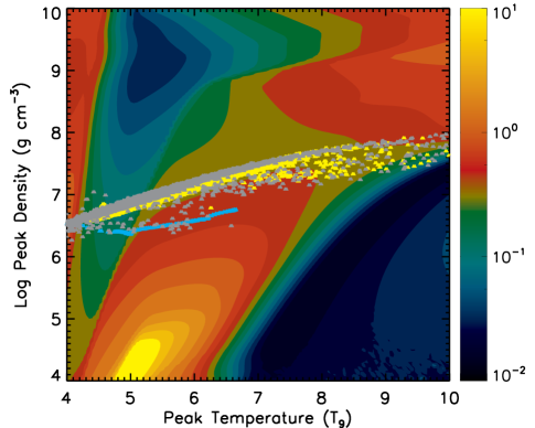
Figure 1.— Final [$\mathrm{{}^{57}Ni}$ / $\mathrm{{}^{56}Ni}$] after freeze-out from exponential thermodynamic trajectories for an electron fraction of $Y_{e}=0.5$ as a function of peak temperature and peak density (Magkotsios et al., 2010, 2011). Over-plotted are the peak thermodynamic conditions reached in three multi-dimensional core-collapse supernova simulations of SN 1987A (cyan: P. Young and C. Fryer, private communication, 2012; yellow: A. Wongwathanarat and T. Janka, private communication, 2012; gray: Wongwathanarat et al. 2010).

Fig. 1 shows $[\mathrm{{}^{57}Ni}/\mathrm{{}^{56}Ni}]$ produced from post-explosion freeze-out expansion calculations for exponential thermodynamic trajectories within a large grid of peak temperatures and peak densities (Magkotsios et al., 2010, 2011). Both $\mathrm{{}^{56}Ni}$ and $\mathrm{{}^{57}Ni}$ belong in the second family of isotopes that are produced during freeze-out expansions (see Table 2 of Magkotsios et al., 2011). Isotopes of the second family become nuclear flow hubs, dominate the final composition, and do not sustain any transition between equilibrium states during the evolution. This implies relatively featureless contour plots of final yields compared to the isotopes of the first family which do undergo a transition between equilibrium states during the evolution. The structure of $[\mathrm{{}^{57}Ni}/\mathrm{{}^{56}Ni}]$ in Fig. 1 stems from a varying, relative efficiency between $\mathrm{{}^{56}Ni}$ and $\mathrm{{}^{57}Ni}$ in absorbing nuclear flows. Overall, the doubly magic nucleus $\mathrm{{}^{56}Ni}$ is the most efficient flow hub among the isotopes of the second family near the magic number 28. The relative strength of $\mathrm{{}^{57}Ni}$ to $\mathrm{{}^{56}Ni}$ in absorbing flow has a weak dependence on the type of freeze-out. In particular, $\mathrm{{}^{57}Ni}$ is not very efficient for the $\alpha p$-rich freeze-out region and parts of the Si-rich and normal freeze-out regions. For the photodisintegration regime at the bottom right part of Fig. 1 neither isotope is produced.

Fig. 1 also shows the peak conditions taken from three multi-dimensional supernova simulations of SN 1987A to constrain the accessible $[\mathrm{{}^{57}Ni}/\mathrm{{}^{56}Ni}]$. Fig. 1 suggests that in these simulations most of the parameterized trajectories produce ratios near or below unity. The total $[\mathrm{{}^{57}Ni}/\mathrm{{}^{56}Ni}]$ ratio of all mass elements from the exponential trajectories are generally are within a factor of $\sim$2 of the ratios found by post-processing the multi-dimensional SN 1987A supernova simulations with the same 489 isotope reaction network used for the parameterized trajectories. These results are consistent with measurements in the 1.5 – 2 range listed in Table 1.

3. The UVOIR light curve

We base our analysis on the UVOIR pseudo-bolometric light curves (i.e., not counting escaping gamma-rays) instead of a wavelength dependent radiative transfer calculation. Fig. 2 shows V-band data to 4334 days (Leibundgut & Suntzeff, 2003; Fransson et al., 2007) and UVOIR data to 1854 days (Suntzeff et al., 1992; Suntzeff, 1997) for SN 1987A. Owing to their long half-lives, the radionuclides $\mathrm{{}^{44}Ti}$, $\mathrm{{}^{55}Fe}$, and $\mathrm{{}^{60}Co}$ mainly affect the bolometric light curve in the later phases after ${\sim}1200$ days. To constrain the mass ejected of these isotopes, we notice the V-band is an approximately constant fraction of the bolometric light between 840 and 1854 days, as shown by the inset of Fig. 2. We construct an approximate bolometric light curve for longer than 1854 days by scaling the V-band by a constant factor of 12.6. This provides an additional ten UVOIR data points at late times that correspond to the ten measured V-band data points shown in Fig. 2.

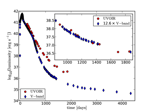
Figure 2.— UVOIR (Suntzeff et al., 1992; Suntzeff, 1997) and V-band (Leibundgut & Suntzeff, 2003; Fransson et al., 2007) light curves for SN 1987A. The inset shows that the V-band is approximately a constant factor of 12.6 the bolometric light curve between 840 and 1854 days. We use this agreement to approximate the UVOIR light from the V-band by assuming the same scaling behavior holds also between days 1854 and 4436.

3.1. Light curve model

We model the bolometric light curve with effective opacities following Woosley et al. (1989); Timmes et al. (1996). We assume that only radioactive energy input contributes to the luminosity and approximately account for energy stored in ionization of the ejecta and released at a later time. We include energy deposited by Auger and internal conversion electrons and we use up to date nuclear decay information from the National Nuclear Data Center (see Table 2). We consider contributions from the following five decay chains to the bolometric supernova light curve:

$${}^{56}\mathrm{Ni}\;\stackrel{{\scriptstyle t_{1/2}=\;6.08d}}{{\hbox to60.0pt{\rightarrowfill}}}\;^{56}\mathrm{Co}\;\stackrel{{\scriptstyle t_{1/2}=\;77.2d}}{{\hbox to60.0pt{\rightarrowfill}}}\;^{56}\mathrm{Fe}$$ (1)

$${}^{57}\mathrm{Ni}\;\stackrel{{\scriptstyle t_{1/2}=\;35.60h}}{{\hbox to60.0pt{\rightarrowfill}}}\;^{57}\mathrm{Co}\;\stackrel{{\scriptstyle t_{1/2}=\;271.79d}}{{\hbox to60.0pt{\rightarrowfill}}}\;^{57}\mathrm{Fe}$$ (2)

$${}^{55}\mathrm{Co}\;\stackrel{{\scriptstyle t_{1/2}=\;17.53h}}{{\hbox to60.0pt{\rightarrowfill}}}\;^{55}\mathrm{Fe}\;\stackrel{{\scriptstyle t_{1/2}=\;999.67d}}{{\hbox to60.0pt{\rightarrowfill}}}\;^{55}\mathrm{Mn}$$ (3)

$${}^{44}\mathrm{Ti}\;\stackrel{{\scriptstyle t_{1/2}=\;58.9y}}{{\hbox to60.0pt{\rightarrowfill}}}\;^{44}\mathrm{Sc}\;\stackrel{{\scriptstyle t_{1/2}=\;3.97h}}{{\hbox to60.0pt{\rightarrowfill}}}\;^{44}\mathrm{Ca}$$ (4)

$${}^{60}\mathrm{Co}\;\stackrel{{\scriptstyle t_{1/2}=\;5.27y}}{{\hbox to60.0pt{\rightarrowfill}}}\;^{60}\mathrm{Ni}$$ (5)

We do not consider the $\mathrm{{}^{22}Na}$ decay chain since nucleosynthesis calculations show the $\mathrm{{}^{55}Co}$ chain always injects significantly more energy than the $\mathrm{{}^{22}Na}$ chain, and $\mathrm{{}^{55}Fe}$ and $\mathrm{{}^{22}Na}$ have very similar half-lives of ${\sim}2.7$ and ${\sim}2.6$ years respectively.

The time-dependence of $n$ nuclide abundances $N_{i}$ in a decay chain is governed by the Bateman equations:

$$\frac{dN_{1}}{dt} = -\lambda_{1}N_{1}$$ (6)

$$\frac{dN_{i}}{dt} = \lambda_{i-1}N_{i-1}-\lambda_{i}N_{i}\enskip.$$ (7)

For $n=2$ and initial abundances $N_{1}(0)$ and $N_{2}(0)$ we get the solution

$$N_{1}(t) = N_{1}(0)\exp(-\lambda_{1}t)$$ (8)

$$N_{2}(t) = N_{1}(0)\frac{\lambda_{1}}{\lambda_{2}-\lambda_{1}}[\exp(-\lambda_{1}t)-\exp(-\lambda_{2}t)]$$

$$+N_{2}(0)\exp(-\lambda_{2}t)\enskip.$$

The decay constants $\lambda_{i}$ are related to the half-lives $t_{1/2,i}$ and the mean life-time $\tau_{i}$ via

$$\lambda_{i}=\frac{1}{\tau_{i}}=\frac{\ln(2)}{t_{1/2,i}}\enskip.$$ (10)

The rate of energy deposition by decays of nucleus $i$ is given by the activity multiplied by the energy deposited per decay:

$$\epsilon_{i}=\lambda_{i}N_{i}(t)q_{i}(t)$$ (11)

where the number $N_{i}$ is given by eq. 8 or eq. 3.1 and the energy deposited, $q_{i}$, is a function of time due to the increasing escape fraction of gamma-rays and possible late time escape of positrons.

To reduce the number of variables we make use of the large difference in half-lives in four of the decay chains

$$\tau(\mathrm{{}^{44}Ti})>>\tau(\mathrm{{}^{44}Sc})$$ (12)

$$\tau(\mathrm{{}^{55}Co})<<\tau(\mathrm{{}^{55}Fe})$$ (13)

$$\tau(\mathrm{{}^{56}Ni})<<\tau(\mathrm{{}^{56}Co})$$ (14)

$$\tau(\mathrm{{}^{57}Ni})<<\tau(\mathrm{{}^{57}Co}).$$ (15)

This allows us to approximate the solution to the Bateman equations with a single exponential for each decay chain. We refer to the luminosity in the $A=44$ chain, where $A$ is the atomic number, as being due to the long-lived $\mathrm{{}^{44}Ti}$, even though the positron is actually produced in the subsequent decay of $\mathrm{{}^{44}Sc}$. Using effective opacities for the gamma-rays and hard X-rays and assuming instantaneous and complete deposition of the leptonic kinetic energy, we obtain the following time-dependent expression for the luminosity due to a given decay chain

$$L_{A}(t)=2.221\ \frac{\lambda_{A}}{A}\frac{\mathrm{M}(A)}{\mathrm{M}_{\odot}}\frac{q^{l}_{A}+q^{\gamma}_{A}f_{A}}{\mathrm{keV}}\exp(-\lambda_{A}t)\times 10^{43}\mathrm{erg}\ ;$$ (16)

where $q^{l}$ and $q^{\gamma}$ are the average energies per decay carried by charged leptons and gamma-rays respectively (see Table 2), $f_{A}=\{1.0-\exp[-\kappa_{A}\phi_{0}(t_{0}/t)^{2}]\}$, $\phi_{0}=7.0\times 10^{4}$ g cm^-2 is the column density at the fiducial time $t_{0}=10^{6}$ s, and $A$ stands for the atomic numbers {44,55,56,57,60} of the five decay chains.

Next, we describe how we take time-dependent freeze-out effects into account (see Fransson & Kozma, 1993, 2002). Freeze-out is most significant in the hydrogen envelope. As recombination times lengthen, the relative importance of freeze-out effects initially increases, as long as gamma-rays still deposit significant energy in the envelope. The $\mathrm{{}^{57}Co}$ and $\mathrm{{}^{60}Co}$ electrons, as well as the $\mathrm{{}^{44}Sc}$ positrons are produced deep in the core and have very short mean free paths. Complete and instantaneous thermalization is therefore still a good approximation for these charged particle contributions. Therefore, upon entering the positron/electron dominated phase, recombination times in the hydrogen envelope become more or less irrelevant, which leads to the disappearance of time-dependent recombination effects. This behavior is clearly shown in figure 2 of Fransson & Kozma (2002), in which time-dependent effects begin to make a difference starting at $\sim$1000 days and increase in importance until $\sim$1600 days. From then on, the difference between the time-dependent and the steady state calculations decreases steadily until $\sim$2800 days when the time-dependent and the steady state results converge again.

We extract the freeze-out contribution $L_{freeze}(t)$ with a plot digitizer from figure 1 of Fransson & Kozma (1993) by taking the difference between the two curves labelled “$\mathrm{{}^{56}Ni}$-only” and extrapolating after 2000 days. We assume a linear dependence of the freeze-out correction on the initial $\mathrm{{}^{56}Ni}$ mass, i.e. the term that is added to the bolometric luminosity is $\tfrac{\mathrm{M}(\mathrm{{}^{56}Ni})}{0.07\,\mathrm{M}_{\odot}}L_{freeze}(t)$. Such a freeze-out correction scaling linearly with M$(\mathrm{{}^{56}Ni})$ appears to be a good approximation since addition of e.g. two times solar $\mathrm{{}^{57}Co}$ does not significantly effect the freeze-out contribution (see figure 1 of Fransson & Kozma 1993). In other words, most of the freeze-out luminosity is energy stored in ionization from the $\mathrm{{}^{56}Co}$ dominated phase, which justifies our approach.

Table 2Charged lepton ($q^{l}$) and gamma-ray ($q^{\gamma}$) partial radioactive decay energies per decay, effective opacities ($\kappa$), and decay constants ($\lambda$).

Nucleus	$\lambda$	$q^{l}$	$q^{\gamma}$	$\kappa$
	[$\mathrm{d}^{-1}$]	[keV]	[keV]	[$\mathrm{cm}^{2}\mathrm{g}^{-1}$]
$\mathrm{{}^{60}Co}$	3.600e-4	96.41	2504	0.04
$\mathrm{{}^{57}Co}$	2.551e-3	17.82	121.6	0.0792
$\mathrm{{}^{56}Co}$	8.975e-3	119.4	3606	0.033
$\mathrm{{}^{55}Fe}$	6.916e-4	3.973	1.635	$\cdots$
$\mathrm{{}^{44}Ti}$	3.222e-5	596.0	2275	0.04

4. Confronting the light curve data with observations and theory

In the previous section, we have constructed a bolometric light curve of SN 1987A from published bolometric data points where available (out to 1854 days) and scaled V-band light at later times. In the following, we use this composite light curve to constrain production masses of radionuclides.

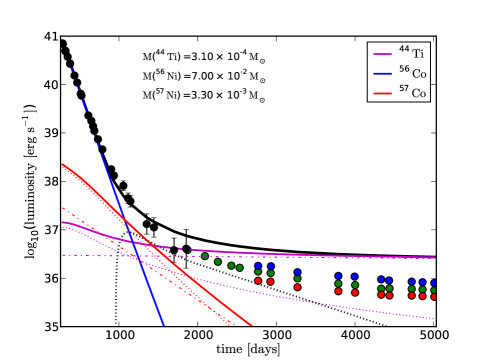
Figure 3.— Model light curve for canonically accepted values of $\mathrm{{}^{56}Ni}$ and $\mathrm{{}^{57}Ni}$ (Fransson & Kozma, 1993) and the $\mathrm{{}^{44}Ti}$ value of Grebenev et al. (2012). The partial $\gamma$-ray contributions for each nuclide are shown with dotted lines and electron and positron contributions are shown with dot-dashed lines. The solid black line is the model bolometric UVOIR luminosity when the energy stored in ionization and released later through recombination is approximately taken into account. The dotted black line shows this freeze-out term, i.e. our model for the delayed release of energy stored in ionization. In black are published UVOIR data for SN 1987A (Suntzeff et al., 1992; Suntzeff, 1997). In green are scaled V-band data (Leibundgut & Suntzeff, 2003; Fransson et al., 2007). Arbitrarily scaled B-band (blue) and R-band (red) data extracted from the paper of Larsson et al. (2011) are shown to demonstrate that a similar rate of decline is present in other optical filters.

We begin with a comparison of our constructed UVOIR light curve with the predictions of our light curve model for canonical production masses of the radionuclides $\mathrm{{}^{56}Ni}$, $\mathrm{{}^{57}Ni}$, and $\mathrm{{}^{44}Ti}$. Fig. 3 shows the model UVOIR light curve and the luminosity of the decay chains using canonical masses of $\mathrm{M}(\mathrm{{}^{56}Ni})=7.0\times 10^{-2}\ \mathrm{M}_{\odot}$ and $\mathrm{M}(\mathrm{{}^{57}Ni})=3.3\times 10^{-3}\ \mathrm{M}_{\odot}$ (Fransson & Kozma, 2002) and the recently determined $\mathrm{M}(\mathrm{{}^{44}Ti})=3.1\times 10^{-4}\ \mathrm{M}_{\odot}$ (Grebenev et al., 2012). Green circles in Fig. 3 are the scaled and time extended V-band data where the scaling corresponds to a constant fraction of $\sim$8% (factor 12.6). Fig. 3 also shows arbitrarily scaled R-band (red circles) and B-band (blue circles) data we extracted from figure 2 of Larsson et al. (2011). Note that B-, V-, and R-band evolve quite similarly: there is apparently not much color evolution during these later epochs. The fact that R- and B-band fall off in a similar manner and bracket the V-band in wavelength lends credence to our extrapolation of the V-band scaling performed in Sec. 3. Note that all color light curves fall off with a time scale much faster than $\mathrm{{}^{44}Ti}$ and that $\mathrm{M}(\mathrm{{}^{44}Ti})=3.1\times 10^{-4}\ \mathrm{M}_{\odot}$ results in a luminosity at late times significantly exceeding our composite light curve.

Next, we perform a non-linear, non-weighted least-squares fit to the logarithm of composite light curve constructed in the previous section. We use SciPy curvefit, which employs the Levenberg-Marquardt (LM) algorithm. We fit the data with the light curve model consisting of the three traditionally employed radionuclides $\mathrm{{}^{56}Ni}$, $\mathrm{{}^{57}Ni}$, and $\mathrm{{}^{44}Ti}$, as well as $\mathrm{{}^{55}Co}$ and $\mathrm{{}^{60}Co}$ and the freeze-out term (see Sec. 3.1). The result of the fit is shown in Fig. 4. For the nickel isotopes, we obtain best fit values of M$(\mathrm{{}^{56}Ni})=(7.1~{}\pm~{}0.3)\times 10^{-2}\,\mathrm{M}_{\odot}$ and M$(\mathrm{{}^{57}Ni})=(4.1~{}\pm~{}1.8)\times 10^{-3}\,\mathrm{M}_{\odot}$. Note that we obtain M$(\mathrm{{}^{44}Ti})=(5.5\pm 1.7)\times 10^{-5}\ \mathrm{M}_{\odot}$, a value much smaller than the INTEGRAL measurement of $(3.1\pm 0.8)\times 10^{-4}\ \mathrm{M}_{\odot}$ (Grebenev et al., 2012), but very similar to what is obtained from explosion models and nuclear reaction network calculations (see Table 1).

The half-lives of $\mathrm{{}^{60}Co}$ and $\mathrm{{}^{55}Fe}$ are quite similar, which introduces a degeneracy for the fitting algorithm. As a result, their best fit values are much smaller than the associated uncertainties. While we use the best fit values of M$(\mathrm{{}^{55}Co})=9.2\times 10^{-6}\mathrm{M}_{\odot}$ and M$(\mathrm{{}^{60}Co})=4.5\times 10^{-8}\mathrm{M}_{\odot}$ for our combined light curve in Fig. 4, we plot the nuclide specific heating terms for the upper limits on the relevant production masses of M$(\mathrm{{}^{55}Co})<7.2\times 10^{-3}\mathrm{M}_{\odot}$ and M$(\mathrm{{}^{60}Co})<1.7\times 10^{-4}\mathrm{M}_{\odot}$.

For SN 1987A, the leptonic channels of $\mathrm{{}^{57}Co}$ (thin red dash-dotted line) play a lesser role compared to the case of thermonuclear supernovae. Nevertheless, their instantaneous, relative contribution to the total bolometric luminosity peaks at 1533 days at 15.5% and constitutes over 10% between 1058 and 2189 days (see Fig. 5). It is interesting to note that the effect of these electron channels on the best fit $[\mathrm{{}^{57}Ni}/\mathrm{{}^{56}Ni}]$ is even larger. If we perform a fit to the light curve with the electron channels of $\mathrm{{}^{57}Co}$ omitted, we obtain $[\mathrm{{}^{57}Ni}/\mathrm{{}^{56}Ni}]~{}=~{}3.8\pm 1.0$, whereas our best fit of the light curve that includes the heating from internal conversion and Auger electrons of $\mathrm{{}^{57}Co}$ yields $[\mathrm{{}^{57}Ni}/\mathrm{{}^{56}Ni}]~{}=~{}2.5\pm 1.1$.

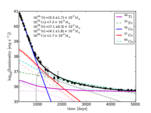
Figure 4.— Model light curve (thick black line) including our time-dependent freeze-out correction (black dashed line). This light curve is the result of a five component least squares fit of initial abundances of $\mathrm{{}^{44}Ti}$, $\mathrm{{}^{56}Ni}$, $\mathrm{{}^{57}Ni}$, $\mathrm{{}^{55}Co}$ and $\mathrm{{}^{60}Co}$ on the composite bolometric light curve constructed in Sec. 3. The partial $\gamma$-ray contributions for each nuclide are shown with dotted lines and electron and positron contributions are shown with dot-dashed lines. The best fit values of $\mathrm{{}^{55}Co}$ and $\mathrm{{}^{60}Co}$ are significantly smaller than their respective uncertainties, which we show as upper limits for these isotopes.

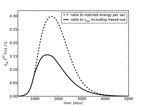
Figure 5.— Relative importance of the $\mathrm{{}^{57}Co}$ electrons for the light curve of SN 1987A. The solid line is the ratio of the energy injection from Auger and internal conversion electrons of $\mathrm{{}^{57}Co}$ (thin red dot-dashed line in Fig. 4) to the total luminosity including freeze-out for our best-fit solution shown in Fig. 4 (solid black line). The dashed line is the ratio of the energy injection from Auger and internal conversion electrons of $\mathrm{{}^{57}Co}$ to the instantaneous total rate of energy injection from radioactive decay (solid black line minus dotted black line in Fig. 4).

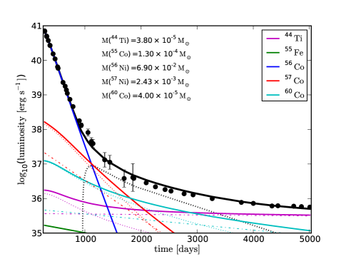
Figure 6.— Model light curve (thick black line) including our time-dependent freeze-out correction (dashed black line) for a choice of initial masses that results in a good fit to the data. For $\mathrm{{}^{44}Ti}$, $\mathrm{{}^{57}Co}$, and $\mathrm{{}^{60}Co}$, gamma-ray (thin dotted lines) and leptonic (thin dash-dotted lines) partial light curves are shown separately as in Figs. 3 and 4.

Fig. 6 demonstrates that a qualitatively good match to the observed light curve is possible where $\mathrm{{}^{60}Co}$ dominates the energy injection in the epoch between the $\mathrm{{}^{57}Co}$ and $\mathrm{{}^{44}Ti}$ dominated phases. Such a scenario is a viable possibility and we advocate that $\mathrm{{}^{60}Co}$ should be included in all late light curve and spectral models of SN 1987A. Again, we have taken the time-dependent effects of freeze-out in the hydrogen envelope approximately into account. This hypothetical model demonstrates that a good match to the light curve data of SN 1987A can be obtained with radionuclides other than $\mathrm{{}^{44}Ti}$ (i.e. $\mathrm{{}^{60}Co}$) dominating the heating at intermediate times.

The luminosity of X-rays produced in the radioactive decays is generally very small compared to the other radiation from decays (e.g. positrons, electrons, gamma-rays) and neglecting X-rays for the heating is therefore generally a good approximation. This ansatz has been made in all previous works that fitted the light curve of SN 1987A. We note, however, that since the decay of $\mathrm{{}^{55}Fe}$ is a ground state to ground state transition, no gamma-rays are emitted and X-rays constitute $\sim$29% of the total liberated decay energy ($\sim$41% of the leptonic contribution). The contribution of X-rays is therefore quite significant for this particular nucleus and for simplicity we work in the limit of full trapping and local thermalization of $\mathrm{{}^{55}Fe}$ X-rays.

5. Summary

We have confirmed previous claims (Seitenzahl, 2011) that the leptonic heating channels (internal conversion and Auger electrons) from the decay of $\mathrm{{}^{57}Co}$ are a significant source of energy for the light curve of SN 1987A, constituting as much as 30% of the instantaneous total rate of energy injection from radioactive decay. For our best-fitting abundances of the radionuclides, the $\mathrm{{}^{57}Co}$ electrons constitute up to 15.5% of the total luminosity at 1533 days (see Fig. 5). Our best fit of the light curve that includes the heating from internal conversion and Auger electrons of $\mathrm{{}^{57}Co}$ yields $[\mathrm{{}^{57}Ni}/\mathrm{{}^{56}Ni}]~{}=~{}2.5\pm 1.1$, down from $[\mathrm{{}^{57}Ni}/\mathrm{{}^{56}Ni}]~{}=~{}3.8\pm 1.0$ for the case where these channels are omitted.

Here we only give upper limits M$(\mathrm{{}^{55}Co})<7.2\times 10^{-3}\mathrm{M}_{\odot}$ and M$(\mathrm{{}^{60}Co})<1.7\times 10^{-4}\mathrm{M}_{\odot}$ on the production masses of the cobalt isotopes. Within the uncertainties of our light curve analysis, an e.g. $\mathrm{{}^{60}Co}$ dominated phase remains a possibility in the epoch between the $\mathrm{{}^{57}Co}$- and $\mathrm{{}^{44}Ti}$-dominated phases. We note, however, that our best fit to the reconstructed bolometric light curve (including the freeze-out term) does not require any significant power from either $\mathrm{{}^{55}Fe}$ or $\mathrm{{}^{60}Co}$.

We investigated the impact of the recently determined $\mathrm{{}^{44}Ti}$ mass of $3.1\times 10^{-4}\ \mathrm{M}_{\odot}$. We find that published, fully reconstructed data is still reconcilable with this high value, but that V-, B-, and R-band at late times indicate that a much lower value would match the light curve better. Indeed, our fit of the constructed bolometric light curve gives M$(\mathrm{{}^{44}Ti})=(0.55\pm 0.17)\times 10^{-4}\,\mathrm{M}_{\odot}$, a value in good agreement with most explosion models and nuclear reaction network calculations.

References

- Anders & Grevesse (1989) Anders, E., & Grevesse, N. 1989, Geochim. Cosmochim. Acta, 53, 197
- Asplund et al. (2009) Asplund, M., Grevesse, N., Sauval, A. J., & Scott, P. 2009, ARA&A, 47, 481
- Borkowski et al. (1997) Borkowski, K. J., de Kool, M., McCray, R., & Wooden, D. H. 1997, BAAS, 29, 1269
- Bouchet & Danziger (1993) Bouchet, P., & Danziger, I. J. 1993, A&A, 273, 451
- Cameron (1982) Cameron, A. G. W. 1982, in Essays in Nuclear Astrophysics, ed. C. A. Barnes, D. D. Clayton, & D. N. Schramm (Cambridge University Press, Cambridge), 23
- Chugai et al. (1997) Chugai, N. N., Chevalier, R. A., Kirshner, R. P., & Challis, P. M. 1997, ApJ, 483, 925
- Dwek et al. (1992) Dwek, E., Moseley, S. H., Glaccum, W., Graham, J. R., Loewenstein, R. F., Silverberg, R. F., & Smith, R. K. 1992, ApJ, 389, L21
- Fransson et al. (2007) Fransson, C., Gilmozzi, R., Groeningsson, P., Hanuschik, R., Kjaer, K., Leibundgut, B., & Spyromilio, J. 2007, The Messenger, 127, 44
- Fransson & Kozma (1993) Fransson, C., & Kozma, C. 1993, ApJ, 408, L25
- Fransson & Kozma (2002) Fransson, C., & Kozma, C. 2002, New A Rev., 46, 487
- Grebenev et al. (2012) Grebenev, S. A., Lutovinov, A. A., Tsygankov, S. S., & Winkler, C. 2012, Nature, 490, 373
- Jerkstrand et al. (2011) Jerkstrand, A., Fransson, C., & Kozma, C. 2011, A&A, 530, A45
- Kumagai et al. (1991) Kumagai, S., Shigeyama, T., Nomoto, K., & Hashimoto, M. 1991, A&A, 243, L13
- Kurfess et al. (1992) Kurfess, J. D., Johnson, W. N., Kinzer, R. L., Kroeger, R. A., Strickman, M. S., Grove, J. E., Leising, M. D., Clayton, D. D., Grabelsky, D. A., Purcell, W. R., Ulmer, M. P., Cameron, R. A., & Jung, G. V. 1992, ApJ, 399, L137
- Larsson et al. (2011) Larsson, J., Fransson, C., Östlin, G., Gröningsson, P., Jerkstrand, A., Kozma, C., Sollerman, J., Challis, P., Kirshner, R. P., Chevalier, R. A., Heng, K., McCray, R., Suntzeff, N. B., Bouchet, P., Crotts, A., Danziger, J., Dwek, E., France, K., Garnavich, P. M., Lawrence, S. S., Leibundgut, B., Lundqvist, P., Panagia, N., Pun, C. S. J., Smith, N., Sonneborn, G., Wang, L., & Wheeler, J. C. 2011, Nature, 474, 484
- Leibundgut & Suntzeff (2003) Leibundgut, B., & Suntzeff, N. B. 2003, in Lecture Notes in Physics, Berlin Springer Verlag, Vol. 598, Supernovae and Gamma-Ray Bursters, ed. K. Weiler, 77–90
- Leising (2006) Leising, M. D. 2006, ApJ, 651, 1019
- Lodders (2003) Lodders, K. 2003, ApJ, 591, 1220
- Lundqvist et al. (2001) Lundqvist, P., Kozma, C., Sollerman, J., & Fransson, C. 2001, A&A, 374, 629
- Magkotsios et al. (2010) Magkotsios, G., Timmes, F. X., Hungerford, A. L., Fryer, C. L., Young, P. A., & Wiescher, M. 2010, ApJS, 191, 66
- Magkotsios et al. (2011) Magkotsios, G., Timmes, F. X., & Wiescher, M. 2011, ApJ, 741, 78
- Motizuki & Kumagai (2004) Motizuki, Y., & Kumagai, S. 2004, New A Rev., 48, 69
- Nagataki et al. (1997) Nagataki, S., Hashimoto, M.-A., Sato, K., & Yamada, S. 1997, ApJ, 486, 1026
- Nagataki et al. (1998) Nagataki, S., Hashimoto, M.-A., Sato, K., Yamada, S., & Mochizuki, Y. S. 1998, ApJ, 492, L45
- Nomoto et al. (2006) Nomoto, K., Tominaga, N., Umeda, H., Kobayashi, C., & Maeda, K. 2006, Nuclear Physics A, 777, 424
- Pinto et al. (1988) Pinto, P. A., Woosley, S. E., & Ensman, L. M. 1988, ApJ, 331, L101
- Rauscher et al. (2002) Rauscher, T., Heger, A., Hoffman, R. D., & Woosley, S. E. 2002, ApJ, 576, 323
- Röpke et al. (2012) Röpke, F. K., Kromer, M., Seitenzahl, I. R., Pakmor, R., Sim, S. A., Taubenberger, S., Ciaraldi-Schoolmann, F., Hillebrandt, W., Aldering, G., Antilogus, P., Baltay, C., Benitez-Herrera, S., Bongard, S., Buton, C., Canto, A., Cellier-Holzem, F., Childress, M., Chotard, N., Copin, Y., Fakhouri, H. K., Fink, M., Fouchez, D., Gangler, E., Guy, J., Hachinger, S., Hsiao, E. Y., Chen, J., Kerschhaggl, M., Kowalski, M., Nugent, P., Paech, K., Pain, R., Pecontal, E., Pereira, R., Perlmutter, S., Rabinowitz, D., Rigault, M., Runge, K., Saunders, C., Smadja, G., Suzuki, N., Tao, C., Thomas, R. C., Tilquin, A., & Wu, C. 2012, ApJ, 750, L19
- Rosman & Taylor (1998) Rosman, K. J. R., & Taylor, P. D. P. 1998, J. Phys. Chem. Ref. Data, 27, 1275
- Seitenzahl (2011) Seitenzahl, I. R. 2011, Prog. Part. Nucl. Phys. 66, 329
- Seitenzahl et al. (2009) Seitenzahl, I. R., Taubenberger, S., & Sim, S. A. 2009, MNRAS, 400, 531
- Suntzeff (1997) Suntzeff, N. B. 1997, arXiv:astro-ph/9707324
- Suntzeff et al. (1992) Suntzeff, N. B., Phillips, M. M., Elias, J. H., Walker, A. R., & Depoy, D. L. 1992, ApJ, 384, L33
- Sunyaev et al. (1991) Sunyaev, R., Grebenev, S., Kaniovsky, A., Efremov, V., Kuznetsov, A., Pavlinsky, M., Yamburenko, N., Englhauser, J., Doebereiner, S., Pietsch, W., Reppin, C., Truemper, J., Kendziorra, E., Maisack, M., Mony, B., & Staubert, R. 1991, in American Institute of Physics Conference Series, Vol. 232, Gamma-Ray Line Astrophysics, ed. P. Durouchoux & N. Prantzos, 211–217
- Thielemann et al. (1996) Thielemann, F.-K., Nomoto, K., & Hashimoto, M.-A. 1996, ApJ, 460, 408
- Timmes et al. (1996) Timmes, F. X., Woosley, S. E., Hartmann, D. H., & Hoffman, R. D. 1996, ApJ, 464, 332
- Tur et al. (2010) Tur, C., Heger, A., & Austin, S. M. 2010, ApJ, 718, 357
- Varani et al. (1990) Varani, G. F., Meikle, W. P. S., Spyromilio, J., & Allen, D. A. 1990, MNRAS, 245, 570
- Wang et al. (1996) Wang, L., Wheeler, J. C., Kirshner, R. P., Challis, P. M., Filippenko, A. V., Fransson, C., Panagia, N., Phillips, M. M., & Suntzeff, N. 1996, ApJ, 466, 998
- Wongwathanarat et al. (2010) Wongwathanarat, A., Janka, H.-T., & Müller, E. 2010, ApJ, 725, L106
- Woosley et al. (1989) Woosley, S. E., Hartmann, D., & Pinto, P. A. 1989, ApJ, 346, 395
- Woosley & Hoffman (1991) Woosley, S. E., & Hoffman, R. D. 1991, ApJ, 368, L31
- Woosley & Weaver (1995) Woosley, S. E., & Weaver, T. A. 1995, ApJS, 101, 181