A Framework of Conjugate Direction Methods for
Symmetric Linear Systems in Optimization

Abstract

In this paper we introduce a parameter dependent class of Krylov-based methods, namely $CD$, for the solution of symmetric linear systems. We give evidence that in our proposal we generate sequences of conjugate directions, extending some properties of the standard Conjugate Gradient (CG) method, in order to preserve the conjugacy. For specific values of the parameters in our framework we obtain schemes equivalent to both the CG and the scaled-CG. We also prove the finite convergence of the algorithms in $CD$, and we provide some error analysis. Finally, preconditioning is introduced for $CD$, and we show that standard error bounds for the preconditioned CG also hold for the preconditioned $CD$.

1 Introduction

The solution of symmetric linear systems arises in a wide range of real applications A96 ; GV89 ; S03 , and has been carefully issued in the last 50 years, due to the increasing demand of fast and reliable solvers. Illconditioning and large number of unknowns are among the most challenging issues which may harmfully affect the solution of linear systems, in several frameworks where either structured or unstructured coefficient matrices are considered A96 ; H96 ; SVdV00 .

The latter facts have required the introduction of a considerable number of techniques, specifically aimed at tackling classes of linear systems with appointed pathologies SVdV00 ; GS92 . We remark that the structure of the coefficient matrix may be essential for the success of the solution methods, both in numerical analysis and optimization contexts. As an example, PDEs and PDE-constrained optimization provide two specific frameworks, where sequences of linear systems often claim for specialized and robust methods, in order to give reliable solutions.

In this paper we focus on iterative Krylov-based methods for the solution of symmetric linear systems, arising in both numerical analysis and optimization contexts. The theory detailed in the paper is not limited to consider large scale linear systems; however, since Krylov-based methods have proved their efficiency when the scale is large, without loss of generality we will implicitly assume the latter fact.

The accurate study and assessment of methods for the solution of linear systems is naturally expected from the community of people working on numerical analysis. That is due to their expertise and great sensibility to theoretical issues, rather than to practical algorithms implementation or software developments. This has raised a consistent literature, including manuals and textbooks, where the analysis of solution techniques for linear systems has become a keynote subject, and where essential achievements have given strong guidelines to theoreticians and practitioners from optimization H96 .

We address here a parameter dependent class of CG-based methods, which can equivalently reduce to the CG for a suitable choice of the parameters. We firmly claim that our proposal is not primarily intended to provide an efficient alternative to the CG. On the contrary, we mainly detail a general framework of iterative methods, inspired by polarity for quadratic hypersurfaces, and based on the generation of conjugate directions. The algorithms in our class, thanks to the parameters in the scheme, may possibly keep under control the conjugacy loss among directions, which is often caused by finite precision in the computation. The paper is not intended to report also a significant numerical experience. Indeed, we think that there are not yet clear rules on the parameters of our proposal, for assessing efficient algorithms. Similarly, we have not currently indications that methods in our proposal can outperform the CG. On this guideline, in a separate paper we will carry on selective numerical tests, considering both symmetric linear systems from numerical analysis and optimization. We further prove that preconditioning can be introduced for the class of methods we propose, as a natural extension of the preconditioned CG (see also GV89 ).

As regards the symbols used in this paper, we indicate with $\lambda_{m}(A)$ and $\lambda_{M}(A)$ the smallest/largest eigenvalue of the positive definite matrix $A$; moreover $\|v\|^{2}_{A}=v^{T}Av$, where $A$ is a positive definite real matrix. $R(A)$ is the range of matrix $A$ and $A^{+}$ is the Moore-Penrose pseudoinverse of matrix $A$. With $Pr_{C}(v)$ we represent the orthogonal projection of vector $v\in\mathbb{R}$ onto the convex set $C\subseteq\mathbb{R}$. Finally, the symbol ${\cal K}_{i}(b,A)$ indicates the Krylov subspace ${\rm span}\{b,Ab,A^{2}b,\dots,A^{i}b\}$ of dimension $i+1$. All the other symbols in the paper follow a standard notation.

Sect. 2 briefly reviews both the CG and the Lanczos process, as Krylov-subspace methods, in order to highlight promising aspects to investigate in our proposal. Sect. 3 details some relevant applications of conjugate directions in optimization frameworks, motivating our interest for possible extensions of the CG. In Sects.  4 and 5 we describe our class of methods and some related properties. In Sects.  6 and 7 we show that the CG and the scaled-CG may be equivalently obtained as particular members of our class. Then, Sects.  8 and 9 contain further properties of the class of methods we propose. Finally, Sect. 10 analyzes the preconditioned version of our proposal, and a section of Conclusions completes the paper, including some numerical results.

2 The CG Method and the Lanczos Process

In this section we comment the method in Table 1, and we focus on the relation between the CG and the Lanczos process, as Krylov-subspace methods. In particular, the Lanczos process namely does not generate conjugate directions; however, though our proposal relies on generalizing the CG, it shares some aspects with the Lanczos iteration, too.
As we said, the CG is commonly used to iteratively solving the linear system

Table 1: The CG algorithm for solving (1).

The Conjugate Gradient (CG) method Step $0$:     Set $k=0$,  $y_{0}\in\mathbb{R}$,  $r_{0}:=b-Ay_{0}$.                 If $r_{0}=0$, then STOP. Else, set $p_{0}:=r_{0}$;  $k=k+1$.                 Set $p_{-1}=0$ and $\beta_{-1}=0$. Step $k$:     Compute $\alpha_{k-1}:=r_{k-1}^{T}p_{k-1}/p_{k-1}^{T}Ap_{k-1}$,                 $y_{k}:=y_{k-1}+\alpha_{k-1}p_{k-1}$,  $r_{k}:=r_{k-1}-\alpha_{k-1}Ap_{k-1}$.                 If $r_{k}=0$, then STOP. Else, set                   –  $\beta_{k-1}:=\|r_{k}\|^{2}/\|r_{k-1}\|^{2}$, $p_{k}:=r_{k}+\beta_{k-1}p_{k-1}$                   –  (or equivalently set $p_{k}:=-\alpha_{k-1}Ap_{k-1}+(1+\beta_{k-1})p_{k-1}-\beta_{k-2}p_{k-2}$)                 Set $k=k+1$, go to Step $k$.

$$Ay=b,$$ (1)

where $A\in\mathbb{R}^{n\times n}$ is symmetric positive definite and $b\in\mathbb{R}^{n}$. Observe that the CG is quite often applied to a preconditioned version of the linear system (1), i.e. ${\cal M}Ay={\cal M}b$, where ${\cal M}\succ 0$ is the preconditioner G97 . Though the theory for the CG requires $A$ to be positive definite, in several practical applications it is successfully used when $A$ is indefinite, too H80 ; Nash2000 . At Step $k$ the CG generates the pair of vectors $r_{k}$ (residual) and $p_{k}$ (search direction) such that GV89

$${\rm orthogonality\ \ property:}\qquad\ r_{i}^{T}r_{j}=0,\qquad\qquad\ \ \ 0\leq i\not=j\leq k,$$ (2)

$${\rm conjugacy\ \ property:}\quad\qquad\ \,p_{i}^{T}Ap_{j}=0,\qquad\qquad 0\leq i\not=j\leq k.$$ (3)

Moreover, finite convergence holds, i.e. $Ay_{h}=b$ for some $h\leq n$. Relations (2) yield the Ritz-Galerkin condition $r_{k}\perp{\cal K}_{k-1}(r_{0},A)$, where

$${\cal K}_{k-1}(r_{0},A):={\rm span}\{b,Ab,A^{2}b,\ldots,A^{k-1}b\}\equiv{\rm span}\{r_{0},\ldots,r_{k-1}\}.$$

Furthermore, the direction $p_{k}$ is computed at Step $k$ imposing the conjugacy condition $p_{k}^{T}Ap_{k-1}=0$. It can be easily proved that the latter equality implicitly satisfies relations (3), with $p_{0},\ldots,p_{k}$ linearly independent. We remark that on practical problems, due to finite precision and roundoff in the computation of the sequences $\{p_{k}\}$ and $\{r_{k}\}$, when $|i-j|$ is large relations (2)-(3) may fail. Thus, in the practical implementation of the CG some theoretical properties may not be satisfied, and in particular when $|i-j|$ increases the conjugacy properties (3) may progressively be lost. As detailed in CGT00 ; F05 ; GLL89 ; MN00 the latter fact may have dramatic consequences also in optimization frameworks (see also Sect. 3 for details). To our purposes we note that in Table 1, at Step $k$ of the CG, the direction $p_{k}$ is usually computed as

$$p_{k}:=r_{k}+\beta_{k-1}p_{k-1},$$ (4)

but an equivalent expression is (see also Theorem 5.4 in HS52 )

$$p_{k}:=-\alpha_{k-1}Ap_{k-1}+(1+\beta_{k-1})p_{k-1}-\beta_{k-2}p_{k-2},$$ (5)

which we would like to generalize in our proposal. Note also that in exact arithmetics the property (3) is iteratively fulfilled by both (4) and (5).

The Lanczos process (and its preconditioned version) is another Krylov-based method, widely used to tridiagonalize the matrix $A$ in (1). Unlike the CG method, here the matrix $A$ may be possibly indefinite, and the overall method is slightly more expensive than the CG, since further computation is necessary to solve the resulting tridiagonal system. Similarly to the CG, the Lanczos process generates at Step $k$ the sequence $\{u_{k}\}$ (Lanczos vectors) which satisfies

$${\rm orthogonality\ \ property:}\qquad u_{i}^{T}u_{j}=0,\qquad 0\leq i\not=j\leq k,$$

and yields finite convergence in at most $n$ steps. However, unlike the CG the Lanczos process is not explicitly inspired by polarity, in order to generate the orthogonal vectors. We recall that the CG and the Lanczos process are 3-term recurrence methods, in other words, for $k\geq 1$

$$\begin{array}[]{l}p_{k+1}\in{\rm span}\{Ap_{k},p_{k},p_{k-1}\},\qquad{\rm for\ the\ CG}\\ \\ u_{k+1}\in{\rm span}\{Au_{k},u_{k},u_{k-1}\},\qquad{\rm for\ the\ Lanczos\ process}.\end{array}$$

When $A$ is positive definite, a full theoretical correspondence between the sequence $\{r_{k}\}$ of the CG and the sequence $\{u_{k}\}$ of the Lanczos process may be fruitfully used in optimization problems (see also CGT00 ; F07 ; S83 ), being

$$u_{k}=s_{k}\frac{r_{k}}{\|r_{k}\|},\qquad\qquad s_{k}\in\{-1,+1\}.$$

The class $CD$ proposed in this paper provides a framework, which encompasses the CG and to some extent resembles the Lanczos iteration, since a 3-term recurrence is exploited. In particular, the $CD$ generates both conjugate directions (as the CG) and orthogonal residuals (as the CG and the Lanczos process). Moreover, similarly to the CG, the $CD$ yields a 3-term recurrence with respect to conjugate directions. As we remarked, our proposal draws its inspiration from the idea of possibly attenuating the conjugacy loss of the CG, which may occur in (3) when $|i-j|$ is large.

3 Conjugate Directions for Optimization Frameworks

Optimization frameworks offer plenty of symmetric linear systems where CG-based methods are often specifically preferable with respect to other solvers. Here we justify this statement by briefly describing the potential use of conjugate directions within truncated Newton schemes. The latter methods strongly prove their efficiency when applied to large scale problems, where they rely on the proper computation of search directions, as well as truncation rules (see NS90 ).
As regards the computation of search directions, suppose at the outer iteration $h$ of the truncated scheme we perform $m$ steps of the CG, in order to compute the approximate solution $d_{h}^{m}$ to the linear system (Newton’s equation)

$$\nabla^{2}f(z_{h})d=-\nabla f(z_{h}).$$

When $z_{h}$ is close enough to the solution $z^{\ast}$ (minimum point) then possibly $\nabla^{2}f(z_{h})\succ 0$. Thus, the conjugate directions $p_{1},\ldots,p_{m}$ and the coefficients $\alpha_{1},\ldots,\alpha_{m}$ are generated as in Table 1, so that the following vectors can be formed

$$\begin{array}[]{lcl}\displaystyle d_{h}^{m}=\sum_{i=1}^{m}\alpha_{i}p_{i},&&\\ \displaystyle d_{h}^{P}=\sum_{i\in I_{h}^{P}}\alpha_{i}p_{i},&&I_{h}^{P}=\left\{i\in\{1,\ldots,m\}:\ \ p_{i}^{T}\nabla^{2}f(z_{h})p_{i}>0\right\},\\ \displaystyle d_{h}^{N}=\sum_{i\in I_{h}^{N}}\alpha_{i}p_{i},&&I_{h}^{N}=\left\{i\in\{1,\ldots,m\}:\ \ p_{i}^{T}\nabla^{2}f(z_{h})p_{i}<0\right\},\\ \displaystyle s_{h}=\frac{p_{\ell}}{\|r_{\ell}\|},&&\displaystyle\ell={\arg\min}_{i\in\{1,\ldots,m\}}\left\{\frac{p_{i}^{T}\nabla^{2}f(z_{h})p_{i}}{\|r_{i}\|^{2}}:\ \ p_{i}^{T}\nabla^{2}f(z_{h})p_{i}<0\right\}.\end{array}$$ (6)

Observe that $d_{h}^{m}$ approximates in some sense Newton’s direction at the outer iteration $h$, and as described in F05 ; GLL89 ; FaRo07 ; GLRT00 the vectors $d_{h}^{m}$, $d_{h}^{P}$ and $d_{h}^{N}$ can be used/combined to provide fruitful search directions to the optimization framework. Moreover, $d_{h}^{N}$ and $s_{h}$ are suitably used/combined to compute a so called negative curvature direction ‘$s_{h}^{m}$’, which can possibly force second order convergence for the overall truncated optimization scheme (see FaRo07 for details). The conjugacy property is essential for computing the vectors (6). i.e. to design efficient truncated Newton methods. Thus, introducing CG-based schemes which deflate conjugacy loss might be of great importance.

On the other hand, at the outer iteration $h$ effective truncation rules typically attempt to assess the parameter $m$ in (6), as described in NS90 ; FaLu09 ; NW00 . I.e., they monitor the decrease of the quadratic local model

$$Q_{h}(d_{h}^{m}):=f(z_{h})+\nabla f(z_{h})^{T}(d_{h}^{m})+\frac{1}{2}(d_{h}^{m})^{T}\nabla^{2}f(z_{h})(d_{h}^{m})$$

when $\nabla^{2}f(z_{h})\succ 0$, so that the parameter $m$ is chosen to satisfy some conditions, including

$$\frac{Q_{h}(d_{h}^{m})-Q_{h}(d_{h}^{m-1})}{Q_{h}(d_{h}^{m})/m}\leq\alpha,\qquad{\rm for\ some\ }\alpha\in\ ]0,1[.$$

Thus, again the correctness of conjugacy properties among the directions $p_{1},\ldots,p_{m}$, generated while solving Newton’s equation, may be essential both for an accurate solution of Newton’s equation (which is a linear system) and to the overall efficiency of the truncated optimization method.

4 Our Proposal: the $CD$ Class

Before introducing our proposal for a new general framework of CG-based algorithms, we consider here some additional motivations for using the CG. The careful use of the latter theory is in our opinion a launching pad for possible extensions of the CG. On this guideline, recalling the contents in Sect. 3, now we summarize some critical aspects of the CG:

1. the CG works iteratively and at any iteration the overall computational effort is only $O(n^{2})$ (since the CG is a Krylov-subspace method);

2. the conjugate directions generated by the CG are linearly independent, so that at most $n$ iterations are necessary to address the solution;

3. the current conjugate direction $p_{k+1}$ is computed by simply imposing the conjugacy with respect to the direction $p_{k}$ (computed) in the previous iteration. This automatically yields that $p_{k+1}^{T}Ap_{i}=0$, for any $i\leq k$, too.

As a matter of fact, for the design of possible general frameworks including CG-based methods, the items 1. and 2. are essential in order to respectively control the computational effort and ensure the finite convergence.

On the other hand, altering the item 3. might be harmless for the overall iterative process, and might possibly yield some fruitful generalizations. That is indeed the case of our proposal, where the item 3. is modified with respect to the CG. The latter modification depends on a parameter which is user/problem-dependent, and may be set in order to further compensate or correct the conjugacy loss among directions, due to roundoff and finite precision.

We sketch in Table 2 our new CG-based class of algorithms, namely $CD$.

Table 2: The parameter dependent class $CD$ of CG-based algorithms for solving (1).

The $CD$ class Step $0$:     Set $k=0$, $y_{0}\in\mathbb{R}^{n}$, $r_{0}:=b-Ay_{0}$, $\gamma_{0}\in\mathbb{R}\setminus\{0\}$.                 If $r_{0}=0$, then STOP. Else, set $p_{0}:=r_{0}$, $k=k+1$.                 Compute $a_{0}:=r_{0}^{T}p_{0}/p_{0}^{T}Ap_{0}$,                 $y_{1}:=y_{0}+a_{0}p_{0}$,  $r_{1}:=r_{0}-a_{0}Ap_{0}$.                 If $r_{1}=0$, then STOP. Else, set $\sigma_{0}:=\gamma_{0}\|Ap_{0}\|^{2}/p_{0}^{T}Ap_{0}$,                 $p_{1}:=\gamma_{0}Ap_{0}-\sigma_{0}p_{0}$,   $k=k+1$. Step $k$:     Compute $a_{k-1}:=r_{k-1}^{T}p_{k-1}/p_{k-1}^{T}Ap_{k-1}$,                 $y_{k}:=y_{k-1}+a_{k-1}p_{k-1}$,  $r_{k}:=r_{k-1}-a_{k-1}Ap_{k-1}$.                 If $r_{k}=0$, then STOP. Else, set $\sigma_{k-1}:=\gamma_{k-1}\frac{\|Ap_{k-1}\|^{2}}{p_{k-1}^{T}Ap_{k-1}}$,                 $\omega_{k-1}:=\gamma_{k-1}\frac{(Ap_{k-1})^{T}Ap_{k-2}}{p_{k-2}^{T}Ap_{k-2}}=\frac{\gamma_{k-1}}{\gamma_{k-2}}\frac{p_{k-1}^{T}Ap_{k-1}}{p_{k-2}^{T}Ap_{k-2}}$,  $\gamma_{k-1}\in\mathbb{R}\setminus\{0\}$                 $p_{k}:=\gamma_{k-1}Ap_{k-1}-\sigma_{k-1}p_{k-1}-\omega_{k-1}p_{k-2}$,  $k=k+1$.                 Go to Step $k$.

The computation of the direction $p_{k}$ at Step $k$ reveals the main difference between the CG and $CD$. In particular, in Table 2 the pair of coefficients $\sigma_{k-1}$ and $\omega_{k-1}$ is computed so that explicitly

$$\begin{array}[]{l}p_{k}^{T}Ap_{k-1}\ =\ 0\\ \\ p_{k}^{T}Ap_{k-2}\ =\ 0,\end{array}$$ (8)

i.e. in Cartesian coordinates the conjugacy between the direction $p_{k}$ and both the directions $p_{k-1}$ and $p_{k-2}$ is directly imposed, as specified by (3). As detailed in Sect. 2, imposing the double condition (8) allows to possibly recover the conjugacy loss in the sequence $\{p_{i}\}$.

On the other hand, the residual $r_{k}$ at Step $k$ of Table 2 is computed by imposing the orthogonality condition $r_{k}^{T}p_{k-1}=0$, as in the standard CG. The resulting method is evidently a bit more expensive than the CG, requiring one additional inner product per step, as long as an additional scalar to compute and an additional $n$-vector to store. From Table 2 it is also evident that $CD$ provides a 3-term recurrence with respect to the conjugate directions.

In addition, observe that the residual $r_{k}$ is computed at Step $k$ of $CD$ only to check for the stopping condition, and is not directly involved in the computation of $p_{k}$. Hereafter in this section we briefly summarize the basic properties of the class $CD$.

Assumption 1

The matrix $A$ in (1) is symmetric positive definite. Moreover, the sequence $\{\gamma_{k}\}$ in Table 2 is such that $\gamma_{k}\not=0$, for any $k\geq 0$.

Note that as for the CG, the Assumption 1 is required for theoretical reasons. However, the $CD$ class may in principle be used also in several cases when $A$ is indefinite, provided that $p_{k}^{T}Ap_{k}\neq 0$, for any $k\geq 0$.

Lemma 1

Let Assumption 1 hold. At Step $k$ of the $CD$ class, with $k\geq 0$, we have

$$Ap_{j}\ \in\ {\rm span}\left\{p_{j+1},p_{j},p_{\max\{0,j-1\}}\right\},\ \ \ \ \ j\leq k.$$ (9)

Proof

From the Step 0 relation (9) holds for $j=0$. Then, for $j=1,\ldots,k-1$ the Step $j+1$ of $CD$ directly yields (9). $\hfill\Box$

Theorem 4.1

[Conjugacy] Let Assumption 1 hold. At Step $k$ of the $CD$ class, with $k\geq 0$, the directions  $p_{0},p_{1},\ldots,p_{k}$ are mutually conjugate, i.e. $p_{i}^{T}Ap_{j}=0$, with $0\leq i\not=j\leq k$.

Proof

The statement holds for Step 0, as a consequence of the choice of the coefficient $\sigma_{0}$. Suppose it holds for $k-1$; then, we have for $j\leq k-1$

$$p_{k}^{T}Ap_{j} = \left(\gamma_{k-1}Ap_{k-1}-\sigma_{k-1}p_{k-1}-\omega_{k-1}p_{k-2}\right)^{T}Ap_{j}$$

$$= (\gamma_{k-1}Ap_{k-1})^{T}Ap_{j}-\sigma_{k-1}p_{k-1}^{T}Ap_{j}-\omega_{k-1}p_{k-2}^{T}Ap_{j}\ =\ 0.$$

In particular, for $j=k-1$ and $j=k-2$ the choice of the coefficients $\sigma_{k-1}$ and $\omega_{k-1}$, and the inductive hypothesis, yield directly $p_{k}^{T}Ap_{k-1}=p_{k}^{T}Ap_{k-2}=0$. For $j<k-2$, the inductive hypothesis and Lemma 1 again yield the conjugacy property. $\hfill\Box$

Lemma 2

Let Assumption 1 hold. Given the $CD$ class, we have for $k\geq 2$

$$(Ap_{k})^{T}(Ap_{i})\ =\ \left\{\begin{array}[]{ccl}\|Ap_{k}\|^{2},&&{\rm if}\ \ i=k,\\ &&\\ \frac{1}{\gamma_{k-1}}p_{k}^{T}Ap_{k},&&{\rm if}\ \ i=k-1,\\ &&\\ \emptyset,&&{\rm if}\ \ i\leq k-2.\end{array}\right.$$

Proof

The statement is a trivial consequence of Step $k$ of the $CD$, Lemma 1 and Theorem 4.1. $\hfill\Box$

Observe that from the previous lemma, a simplified expression for the coefficient $\omega_{k-1}$, at Step $k$ of $CD$ is available, inasmuch as

$$\omega_{k-1}\ =\ \frac{\gamma_{k-1}}{\gamma_{k-2}}\cdot\frac{p_{k-1}^{T}Ap_{k-1}}{p_{k-2}^{T}Ap_{k-2}}.$$ (10)

Relation (10) has a remarkable importance: it avoids the storage of the vector $Ap_{k-2}$ at Step $k$, requiring only the storage of the quantity $p_{k-2}^{T}Ap_{k-2}$. Also observe that unlike the CG, the sequence $\{p_{k}\}$ in $CD$ is computed independently of the sequence $\{r_{k}\}$. Moreover, as we said the residual $r_{k}$ is simply computed at Step $k$ in order to check the stopping condition for the algorithm.

The following result proves that the $CD$ class recovers the main theoretical properties of the standard CG.

Theorem 4.2

[Orthogonality] Let Assumption 1 hold. Let $r_{k+1}\not=0$ at Step $k+1$ of the $CD$ class, with $k\geq 0$. Then, the directions $p_{0},p_{1},\ldots,p_{k}$ and the residuals $r_{0},r_{1},\ldots,r_{k+1}$ satisfy

$$r_{k+1}^{T}p_{j}\ =\ 0,\ \ \ \ \ \ \ \ \ \ j\leq k,$$ (11)

$$r_{k+1}^{T}r_{j}\ =\ 0,\ \ \ \ \ \ \ \ \ \ j\leq k.$$ (12)

Proof

From Step $k+1$ of $CD$ we have $r_{k+1}=r_{k}-a_{k}Ap_{k}=r_{j}-\sum_{i=j}^{k}a_{i}Ap_{i}$, for any $j\leq k$. Then, from Theorem 4.1 and the choice of coefficient $\alpha_{j}$ we obtain

$$r_{k+1}^{T}p_{j}\ =\ \left(r_{j}-\sum_{i=j}^{k}a_{i}Ap_{i}\right)^{T}p_{j}\ =\ r_{j}^{T}p_{j}-\sum_{i=j}^{k}a_{i}p_{i}^{T}Ap_{j}\ =\ 0,\ \ \ \ \ \ \ \ j\leq k,$$

which proves (11). As regards relation (12), for $k=0$ we obtain from the choice of $a_{0}$

$$r_{1}^{T}r_{0}\ =\ r_{1}^{T}p_{0}\ =\ 0.$$

Then, assuming by induction that (12) holds for $k-1$, we have

$$r_{k+1}^{T}r_{j} = \left(r_{k}-a_{k}Ap_{k}\right)^{T}r_{j}\ =\ \left(r_{k}-a_{k}Ap_{k}\right)^{T}\left(r_{0}-\sum_{i=0}^{j-1}a_{i}Ap_{i}\right)$$

$$= r_{k}^{T}r_{0}-\sum_{i=0}^{j-1}a_{i}r_{k}^{T}Ap_{i}-a_{k}p_{k}^{T}Ar_{0}+\sum_{i=0}^{j-1}a_{i}a_{k}(Ap_{k})^{T}Ap_{i},\ \ \ \ \ \ \ \ \ j\leq k.$$

The inductive hypothesis and Theorem 4.1 yield for $j\leq k$ (in the next relation when $i=0$ then $p_{i-1}\equiv 0$)

$$r_{k+1}^{T}r_{j}\ =\ -\sum_{i=0}^{j-1}\frac{a_{i}r_{k}^{T}}{\gamma_{i}}\left(p_{i+1}+\sigma_{i}p_{i}+\omega_{i}p_{i-1}\right)+\sum_{i=0}^{j-1}a_{i}a_{k}(Ap_{k})^{T}Ap_{i}.$$ (13)

Therefore, if $j=k$ the relation (11) along with Lemma 2 and the choice of $a_{k}$ yield

$$r_{k+1}^{T}r_{k} = -\frac{a_{k-1}}{\gamma_{k-1}}r_{k}^{T}p_{k}+\frac{a_{k-1}a_{k}}{\gamma_{k-1}}p_{k}^{T}Ap_{k}\ =\ 0.$$

On the other hand, if $j<k$ in (13), the inductive hypothesis, relation (11) and Lemma 2 yield (12). $\hfill\Box$

Finally, we prove that likewise the CG, in at most $n$ iterations $CD$ determines the solution of the linear system (1), so that finite convergence holds.

Lemma 3

[Finite convergence] Let Assumption 1 hold. At Step $k$ of the $CD$ class, with $k\geq 0$, the vectors $p_{0},\ldots,p_{k}$ are linearly independent. Moreover, in at most $n$ iterations the $CD$ class computes the solution of the linear system (1), i.e. $Ay_{h}=b$, for some $h\leq n$.

Proof

The proof follows very standard guidelines (the reader may also refer to M06 ). Thus, by (11) an integer $m\leq n$ exists such that $r_{m}=b-Ay_{m}=0$. Then, if $y^{\ast}$ is the solution of (1), we have

$$0=b-Ay_{m}=Ay^{\ast}-A\left[y_{0}+\sum_{i=0}^{m-1}a_{i}p_{i}\right]\qquad\Longleftrightarrow\qquad y^{\ast}=y_{0}+\sum_{i=0}^{m-1}a_{i}p_{i}.$$

$\hfill\Box$

Remark 1

Observe that there is the additional chance to replace the Step 0 in Table 2, with the following CG-like Step $0_{b}$

Step $0_{b}$:  Set $k=0$, $y_{0}\in\mathbb{R}^{n}$, $r_{0}:=b-Ay_{0}$.
If $r_{0}=0$, then STOP. Else, set $p_{0}:=r_{0}$,  $k=k+1$.
Compute $a_{0}:=r_{0}^{T}p_{0}/p_{0}^{T}Ap_{0}$,
$y_{1}:=y_{0}+a_{0}p_{0}$,  $r_{1}:=r_{0}-a_{0}Ap_{0}$.
If $r_{1}=0$, then STOP. Else, set $\sigma_{0}:=-\|r_{1}\|^{2}/\|r_{0}\|^{2}$,
$p_{1}:=r_{1}+\sigma_{0}p_{0}$,   $k=k+1$.

5 Further Properties for $CD$

In this section we consider some properties of $CD$ which represent a natural extension of analogous properties of the CG. To this purpose we introduce the error function

$$f(y):=\frac{1}{2}(y-y^{\ast})^{T}A(y-y^{\ast}),\qquad{\rm with}\quad Ay^{\ast}=b,$$ (14)

and the quadratic functional

$$g(y):=\frac{1}{2}(y-y_{i})^{T}A(y-y_{i}),\qquad{\rm with}\quad i\in\{1,\dots,m\},$$ (15)

which satisfy $f(y)\geq 0$, $g(y)\geq 0$, for any $y\in\mathbb{R}^{n}$, when $A\succeq 0$. Then, we have the following result, where we prove minimization properties of the error function $f(y)$ (see also Theorem 6.1 in HS52 ) and $g(y)$ (see also P87 ), along with the fact that $CD$ provides a suitable approximation of the inverse matrix $A^{-1}$, too.

Theorem 5.1

[Further Properties] Consider the linear system (1) with $A\succeq 0$, and the functions $f(y)$ and $g(y)$ in (14)-(15). Assume that the $CD$ has performed $m+1$ iterations, with $m+1\leq n$ and $Ay_{m+1}=b$. Let $\gamma_{i-1}\neq 0$ with $i\geq 1$. Then,

• $\sigma_{0}$ minimizes $g(y)$ on the manifold $(y_{1}+\gamma_{0}Ap_{0})+{\rm span}\{p_{0}\}$,

• $\sigma_{i-1}$ and $\omega_{i-1}$, $i=2,\dots,m$, minimize $g(y)$ on the two dimensional manifold $(y_{i}+\gamma_{i-1}Ap_{i-1})+{\rm span}\{p_{i-1},p_{i-2}\}$.

Moreover,

$$\quad f(y_{i}+a_{i}p_{i})=f(y_{i})-\left(\frac{\gamma_{i-1}}{a_{i-1}}\right)^{2}\frac{\|r_{i}\|^{4}}{p_{i}^{T}Ap_{i}},\qquad i=1,\dots,m,$$ (16)

and we have

$$\left[A^{+}-\sum_{i=0}^{m}\frac{p_{i}p_{i}^{T}}{p_{i}^{T}Ap_{i}}\right]r_{0}=0,\qquad\qquad{\rm for\ any\ }y_{0}\in\mathbb{R}^{n}.$$ (17)

Proof

Observe that for $i=1$, indicating in Table 2  $p_{1}=\gamma_{0}Ap_{0}+ap_{0}$, with $a\in\mathbb{R}$, by (15)

$$g(y_{2})=g(y_{1}+a_{1}p_{1})=\frac{a_{1}^{2}}{2}(\gamma_{0}Ap_{0}+ap_{0})^{T}A(\gamma_{0}Ap_{0}+ap_{0})$$

and we have

$$0=\left.\frac{\partial g(y_{2})}{\partial a}\right|_{a=a^{\ast}}=a_{1}^{2}p_{0}^{T}A(\gamma_{0}Ap_{0}+a^{\ast}p_{0})\quad\Longleftrightarrow\quad a^{\ast}=-\gamma_{0}\frac{\|Ap_{0}\|^{2}}{p_{0}^{T}ap_{0}}=-\sigma_{0}.$$

For $i\geq 2$, if we indicate in Table 2  $p_{i}=\gamma_{i-1}Ap_{i-1}+bp_{i-1}+cp_{i-2}$, with $b,c\in\mathbb{R}$, then by (15)

$$g(y_{i}+a_{i}p_{i}) =\frac{a_{i}^{2}}{2}(\gamma_{i-1}Ap_{i-1}+bp_{i-1}+cp_{i-2})^{T}A(\gamma_{i-1}Ap_{i-1}+bp_{i-1}+cp_{i-2})$$

and by Assumption 1, after some computation, the equalities

$$\left\{\displaystyle\begin{array}[]{l}\displaystyle\left.\frac{\partial g(y_{i+1})}{\partial b}\right|_{b=b^{\ast},\ c=c^{\ast}}=\left.\frac{\partial g(y_{i}+a_{i}p_{i})}{\partial b}\right|_{b=b^{\ast},\ c=c^{\ast}}=0\\ \\ \displaystyle\left.\frac{\partial g(y_{i+1})}{\partial c}\right|_{b=b^{\ast},\ c=c^{\ast}}=\left.\frac{\partial g(y_{i}+a_{i}p_{i})}{\partial c}\right|_{b=b^{\ast},\ c=c^{\ast}}=0\end{array}\right.$$

imply the unique solution

$$\left\{\displaystyle\begin{array}[]{l}\displaystyle b^{\ast}=-\gamma_{i-1}\frac{\|Ap_{i-1}\|^{2}}{p_{i-1}^{T}Ap_{i-1}}=-\sigma_{i-1}\\ \\ \displaystyle c^{\ast}=-\gamma_{i-1}\frac{(Ap_{i-1})^{T}(Ap_{i-2})}{p_{i-2}^{T}Ap_{i-2}}=-\frac{\gamma_{i-1}}{\gamma_{i-2}}\frac{p_{i-1}^{T}Ap_{i-1}}{p_{i-2}^{T}Ap_{i-2}}=-\omega_{i-1}.\end{array}\right.$$ (18)

As regards (16), from Table 2 we have that for any $i\geq 1$

$$f(y_{i}+a_{i}p_{i}) = f(y_{i})+a_{i}(y_{i}-y^{\ast})^{T}Ap_{i}+\frac{1}{2}a_{i}^{2}p_{i}^{T}Ap_{i}$$ (19)

$$= f(y_{i})-a_{i}r_{i}^{T}p_{i}+\frac{1}{2}a_{i}^{2}p_{i}^{T}Ap_{i}$$

$$= f(y_{i})-\frac{1}{2}\frac{(r_{i}^{T}p_{i})^{2}}{p_{i}^{T}Ap_{i}}.$$

Now, since $r_{i}=r_{i-1}-a_{i-1}Ap_{i-1}$ we have

$$p_{i} = \gamma_{i-1}\left(\frac{r_{i-1}-r_{i}}{a_{i-1}}\right)-\sigma_{i-1}p_{i-1},\qquad\qquad\qquad\quad\ \!i=1,$$

$$p_{i} = \gamma_{i-1}\left(\frac{r_{i-1}-r_{i}}{a_{i-1}}\right)-\sigma_{i-1}p_{i-1}-\omega_{i-1}p_{i-2},\qquad i\geq 2,$$

so that from Theorem 4.2

$$r_{i}^{T}p_{i}=-\frac{\gamma_{i-1}}{a_{i-1}}\|r_{i}\|^{2}.$$

The latter relation and (19) yield (16).

As regards (17), since $Ay_{m+1}=b$ then $b\in R(A)$, and from Table 2 then $r_{i}\in{\cal K}_{i}(b,A)\subseteq R(A)$, $i=0,\dots,m$, where ${\cal K}_{i+1}(b,A)\supseteq{\cal K}_{i}(b,A)$. In addition, by the definition of Moore-Penrose pseudoinverse matrix (see CM79 ), and since $y_{m+1}$ is a solution of (1) we have

$$Pr_{R(A)}(y_{m+1}) = A^{+}b\ =\ A^{+}(r_{0}+Ay_{0})$$ (20)

$$= A^{+}r_{0}+Pr_{R(A)}(y_{0}).$$

Moreover, $y_{m+1}=y_{0}+\sum_{i=0}^{m}a_{i}p_{i}$ and by induction $p_{i}\in{\cal K}_{i}(b,A)\subseteq R(A)$, thus

$$Pr_{R(A)}(y_{m+1}) = Pr_{R(A)}(y_{0})+Pr_{R(A)}\left(\sum_{i=0}^{m}a_{i}p_{i}\right)$$ (21)

$$= Pr_{R(A)}(y_{0})+\sum_{i=0}^{m}a_{i}p_{i}.$$

By (20), (21) and recalling that for $CD$ we have $p_{i}^{T}r_{i}=p_{i}^{T}(r_{i-1}-a_{i-1}Ap_{i-1})=p_{i}^{T}r_{i-1}=\cdots=p_{i}^{T}r_{0}$, we obtain

$$A^{+}r_{0}=\sum_{i=0}^{m}a_{i}p_{i}=\sum_{i=0}^{m}\frac{p_{i}^{T}r_{i}}{p_{i}^{T}Ap_{i}}p_{i}=\sum_{i=0}^{m}\frac{p_{i}p_{i}^{T}}{p_{i}^{T}Ap_{i}}r_{0},$$

which yields (17). $\hfill\Box$

Observe that the result in (18) may be seen as a consequence of the Theorem 3.6 in H80 , which holds for a general quadratic functional $g(x)$.

Corollary 1

[Inverse Approximation] Let Assumption 1 hold and suppose that $Ay_{m+1}=b$, where $y_{m+1}$ is computed by $CD$ and $m=n-1$. Then, we have

$$A^{-1}=\sum_{i=0}^{n-1}\frac{p_{i}p_{i}^{T}}{p_{i}^{T}Ap_{i}}.$$

Proof

The proof follows from (17), recalling that the directions $p_{0},\dots,p_{n-1}$ are linearly independent and when $A$ is nonsingular $A^{-1}\equiv A^{+}$. $\hfill\Box$

6 Basic Relation Between the CG and $CD$

Observe that the geometry of vectors $\{p_{k}\}$ and $\{r_{k}\}$ in $CD$ might be substantially different with respect to the CG. Indeed, in the latter scheme the relation $p_{k}=r_{k}+\beta_{k-1}p_{k-1}$ implies $r_{k}^{T}p_{k}=\|r_{k}\|^{2}>0$, for any $k$. On the contrary, for the $CD$, using relation $r_{k}=r_{k-1}-a_{k-1}Ap_{k-1}$ and Theorem 4.2 we have that possibly $r_{k}^{T}p_{k}\neq\|r_{k}\|^{2}$ and

$$\frac{p_{k}^{T}Ap_{k}}{p_{k-1}^{T}Ap_{k-1}} = \gamma_{k-1}\frac{(Ap_{k-1})^{T}Ap_{k}}{p_{k-1}^{T}Ap_{k-1}}\ =\ -\frac{\gamma_{k-1}\|r_{k}\|^{2}}{a_{k}a_{k-1}p_{k-1}^{T}Ap_{k-1}}$$

$$= -\gamma_{k-1}\frac{\|r_{k}\|^{2}p_{k}^{T}Ap_{k}}{(r_{k}^{T}p_{k})(r_{k-1}^{T}p_{k-1})},$$

so that when $A\succ 0$ we obtain

$$\gamma_{k-1}(r_{k}^{T}p_{k})(r_{k-1}^{T}p_{k-1})<0.$$ (22)

The latter result is a consequence of the fact that in the $CD$ class, the direction $p_{k}$ is not generated directly using the vector $r_{k}$. In addition, a similar conclusion also holds if we compute the quantity $p_{k}^{T}p_{j}>0$, $k\not=j$, for both the CG and the $CD$ (see also Theorem 5.3 in HS52 ).

As another difference between the CG and $CD$, we have that in the first algorithm the coefficient $\beta_{k-1}$, at Step $k$ in Table 1, is always positive. On the other hand, the coefficients $\gamma_{k-1}$, $\sigma_{k-1}$ and $\omega_{k-1}$ at Step $k$ of Table 2 might be possibly negative.

We also observe that the CG in Table 1 simply stores at Step $k$ the vectors $r_{k-1}$ and $p_{k-1}$, in order to compute respectively $r_{k}$ and $p_{k}$. On the other hand, at Step $k$ the $CD$ requires the storage of one additional vector, which contains some information from iteration $k-2$. The idea of storing at Step $k$ some information from iterations preceding Step $k-1$ is not new for Krylov-based methods. Some examples, which differ from our approach, may be found in G97 , for unsymmetric linear systems.

In any case, it is not difficult to verify that the CG may be equivalently obtained from $CD$, setting $\gamma_{k-1}=-\alpha_{k-1}$, for $k=1,2,\ldots$, in Table 2. Indeed, though in Table 1 the coefficient $\beta_{k-1}$ explicitly imposes the conjugacy only between $p_{k}$ and $p_{k-1}$, the pair $(\alpha_{k-1},\beta_{k-1})$ implicitly imposes both the conditions (8) for the CG. Now, by (5) and comparing with Step $k$ of Table 2, we want to show that setting $\gamma_{k-1}=-\alpha_{k-1}$ in Table 2 we obtain

$$\left\{\begin{array}[]{lcl}\sigma_{k-1}=-(1+\beta_{k-1}),&&k\geq 1,\\ &&\\ \omega_{k-1}=\beta_{k-2},&&k\geq 2,\end{array}\right.$$ (23)

which implies that $CD$ reduces equivalently to the CG.
For the CG $r_{i}^{T}r_{j}=0$, for $i\not=j$, and $p_{i}^{T}r_{i}=\|r_{i}\|^{2}$, so that

$$\beta_{k-1}:=\frac{\|r_{k}\|^{2}}{\|r_{k-1}\|^{2}}=-\frac{r_{k}^{T}(\alpha_{k-1}Ap_{k-1})}{\|r_{k-1}\|^{2}}=-\frac{r_{k}^{T}Ap_{k-1}}{p_{k-1}^{T}Ap_{k-1}}.$$

Thus, recalling that $r_{k-1}=r_{k-2}-\alpha_{k-2}Ap_{k-2}$ and $p_{k-1}=r_{k-1}+\beta_{k-2}p_{k-2}$, we obtain for $\gamma_{k-1}=-\alpha_{k-1}$, with $k\geq 2$,

$$-(1+\beta_{k-1}) = -\frac{p_{k-1}^{T}Ap_{k-1}-r_{k}^{T}Ap_{k-1}}{p_{k-1}^{T}Ap_{k-1}}$$ (24)

$$= -\frac{(p_{k-1}-r_{k-1}+\alpha_{k-1}Ap_{k-1})^{T}Ap_{k-1}}{p_{k-1}^{T}Ap_{k-1}}$$

$$= -\alpha_{k-1}\frac{\|Ap_{k-1}\|^{2}}{p_{k-1}^{T}Ap_{k-1}}\ =\ \sigma_{k-1}$$

and

$$\beta_{k-2} = -\frac{r_{k-1}^{T}Ap_{k-2}}{p_{k-2}^{T}Ap_{k-2}}\ =\ \frac{\|r_{k-1}\|^{2}}{\alpha_{k-2}}\frac{1}{p_{k-2}^{T}Ap_{k-2}}$$ (25)

$$= \frac{\alpha_{k-1}}{\alpha_{k-2}}\frac{p_{k-1}^{T}Ap_{k-1}}{p_{k-2}^{T}Ap_{k-2}}\ =\ \omega_{k-1}.$$

Finally, it is worth noticing that for $CD$ the following two properties hold, for any $k\geq 2$ ((i)-(ii) also hold for $k=1$, with obvious modifications to (i)):

• $\quad\displaystyle r_{k}^{T}p_{k}=r_{k}^{T}\left[\gamma_{k-1}\left(\frac{r_{k-1}-r_{k}}{a_{k-1}}\right)-\sigma_{k-1}p_{k-1}-\omega_{k-1}p_{k-2}\right]=-\frac{\gamma_{k-1}}{a_{k-1}}\|r_{k}\|^{2}$

• $\quad\displaystyle r_{k}^{T}Ap_{k}=r_{k}^{T}\left(\frac{r_{k}-r_{k+1}}{a_{k}}\right)=\frac{1}{a_{k}}\|r_{k}\|^{2}=\frac{\|r_{k}\|^{2}}{r_{k}^{T}p_{k}}p_{k}^{T}Ap_{k}$,

which indicate explicitly a difference with respect to the CG. Indeed, for any $\gamma_{k-1}\not=-a_{k-1}$ we have respectively from (i) and (ii)

$$\begin{array}[]{c}r_{k}^{T}p_{k}\not=\|r_{k}\|^{2}\\ \\ r_{k}^{T}Ap_{k}\not=p_{k}^{T}Ap_{k}.\end{array}$$

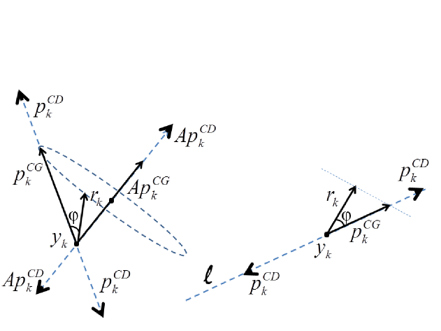
Figure 1: At the $k$th iteration of the CG and $CD$, the directions $p_{k}^{CG}$ and $p_{k}^{CD}$ are respectively generated, along the line $\ell$. Applying the CG, the vectors $p_{k}^{CG}$ and $r_{k}$ have the same orthogonal projection on $Ap_{k}^{CG}$, since $(p_{k}^{CG})^{T}Ap_{k}^{CG}=r_{k}^{T}Ap_{k}^{CG}$. Applying $CD$, the latter equality with $p_{k}^{CD}$ in place of $p_{k}^{CG}$ is not necessarily satisfied

Figure 1 clarifies the geometry of items (i) and (ii) for both the CG and $CD$.
Relations (24)-(25) suggest that the sequence $\{\gamma_{k}\}$ must satisfy specific conditions in order to reduce $CD$ equivalently to the CG. For a possible generalization of the latter conclusion, consider that equalities (23) are by (5) sufficient conditions in order to reduce $CD$ equivalently to the CG. Thus, now we want to study general conditions on the sequence $\{\gamma_{k}\}$, such that (23) are satisfied. By (23) we have

$$-(1+\omega_{k})=\sigma_{k-1},$$

which is equivalent from Table 2 to

$$-\left(\gamma_{k-1}\|Ap_{k-1}\|^{2}+p_{k-1}^{T}Ap_{k-1}\right)=\frac{\gamma_{k}}{\gamma_{k-1}}p_{k}^{T}Ap_{k}$$ (26)

or

$$-\gamma_{k-1}^{2}\|Ap_{k-1}\|^{2}-\gamma_{k-1}p_{k-1}^{T}Ap_{k-1}-\gamma_{k}p_{k}^{T}Ap_{k}=0.$$ (27)

The latter equality, for $k\geq 1$, and the choice of $\sigma_{0}$ in Table 2 yield the following conclusions.

Table 3: The new $CD$-red class for solving (1), obtained by setting at Step $k$ of $CD$ the parameter $\gamma_{k}$ as in relation (28).

The $CD$-red class Step $0$:     Set $k=0$, $y_{0}\in\mathbb{R}^{n}$, $r_{0}:=b-Ay_{0}$.                 If $r_{0}=0$, then STOP. Else, set $p_{0}:=r_{0}$, $k=k+1$.                 Compute $a_{0}:=r_{0}^{T}p_{0}/p_{0}^{T}Ap_{0}$,  $\gamma_{0}:=-a_{0}$,                 $y_{1}:=y_{0}+a_{0}p_{0}$,  $r_{1}:=r_{0}-a_{0}Ap_{0}$.                 If $r_{1}=0$, then STOP. Else, set $\sigma_{0}:=\gamma_{0}\|Ap_{0}\|^{2}/p_{0}^{T}Ap_{0}$,  $\beta_{0}=-(1+\sigma_{0})$                 $p_{1}:=r_{1}+\beta_{0}p_{0}$,   $k=k+1$. Step $k$:     Compute $a_{k-1}:=r_{k-1}^{T}p_{k-1}/p_{k-1}^{T}Ap_{k-1}$,                 $y_{k}:=y_{k-1}+a_{k-1}p_{k-1}$,  $r_{k}:=r_{k-1}-a_{k-1}Ap_{k-1}$.                 If $r_{k}=0$, then STOP. Else, use (28) to compute $\gamma_{k-1}$.                 Set $\sigma_{k-1}:=\gamma_{k-1}\frac{\|Ap_{k-1}\|^{2}}{p_{k-1}^{T}Ap_{k-1}}$,  $\beta_{k-1}:=-(1+\sigma_{k-1})$                 $p_{k}:=r_{k}+\beta_{k-1}p_{k-1}$,  $k=k+1$.                 Go to Step $k$.

Lemma 4

[Reduction of $CD$] The scheme $CD$ in Table 2 can be rewritten as in Table 3 (i.e. with the CG-like structure of Table 1), provided that the sequence $\{\gamma_{k}\}$ satisfies $\gamma_{0}:=-a_{0}$ and

$$\gamma_{k}:=-\frac{\gamma_{k-1}^{2}\|Ap_{k-1}\|^{2}+\gamma_{k-1}p_{k-1}^{T}Ap_{k-1}}{p_{k}^{T}Ap_{k}},\qquad k\geq 1.$$ (28)

In particular, the positions $\gamma_{i}=-a_{i}$, $i\geq 0$, in $CD$ satisfy (28).

Proof

By the considerations which led to (26)-(27), relation (28) yields (23), so that the scheme $CD$-red in Table 3 follows from $CD$ with the position (28), and setting $\gamma_{0}=-a_{0}$.
Furthermore, replacing in (28) the conditions $\gamma_{i}=-a_{i}$, $i\geq 1$, and recalling (i)-(ii), we obtain the condition $a_{k-1}^{2}\|Ap_{k-1}\|^{2}=\|r_{k-1}\|^{2}+\|r_{k}\|^{2}$, which is immediately fulfilled using condition $r_{k}=r_{k-1}-a_{k-1}Ap_{k-1}$. $\hfill\Box$

Note that the $CD$-red scheme substantially is more similar to the CG than to $CD$. Indeed the conditions (8), explicitly imposed at Step $k$ of $CD$, reduce to the unique condition $p_{k}^{T}Ap_{k-1}=0$ in $CD$-red.
The following result is a trivial consequence of Lemma 3, where the alternate use of CG and $CD$ steps is analyzed.

Lemma 5

[Combined Finite Convergence] Let Assumption 1 hold. Let $y_{1},\ldots,y_{h}$ be the iterates generated by $CD$, with $h\leq n$ and $Ay_{h}=b$. Then, finite convergence is preserved (i.e. $Ay_{h}=b$) if the Step $\hat{k}$ of $CD$, with $\hat{k}\in\{k_{1},\ldots,k_{h}\}\subseteq\{1,\ldots,h\}$, is replaced by the Step $\hat{k}$ of the CG.

Proof

First observe that both in Table 1 and Table 2, for any $k\leq h$, the quantity $\|r_{k}\|>0$ is computed. Thus, in Table 1 the coefficient $\beta_{k-1}$ is well defined for any $n>k\geq 1$. Now, by Table 2, setting at Step $\hat{k}\in\{k_{1},\ldots,k_{h}\}\subseteq\{1,\ldots,h\}$ the following

$$\left\{\begin{array}[]{lcl}\gamma_{\hat{k}-1}=-a_{\hat{k}-1}&&{\rm if\ }\hat{k}\geq 1\\ \\ \sigma_{\hat{k}-1}=-(1+\beta_{\hat{k}-1})&&{\rm if\ }\hat{k}\geq 1\\ \\ \omega_{\hat{k}-1}=\beta_{\hat{k}-2}&&{\rm if\ }\hat{k}\geq 2,\\ \end{array}\right.$$

the Step $\hat{k}$ of $CD$ coincides formally with the Step $\hat{k}$ of CG. Thus, finite convergence with $Ay_{h}=b$ is proved recalling that Lemma 3 holds for any choice of the sequence $\{\gamma_{k}\}$, with $\gamma_{k}\not=0$. $\hfill\Box$

7 Relation Between the Scaled-CG and $CD$

Similarly to the previous section, here we aim at determining the relation between our proposal in Table 2 and the scheme of the scaled-CG in Table 4 (see also H80 , page 125).

Table 4: The scaled-CG algorithm for solving (1).

The Scaled-CG method Step $0$:     Set $k=0$,  $y_{0}\in\mathbb{R}$,  $r_{0}:=b-Ay_{0}$.                 If $r_{0}=0$, then STOP. Else, set $p_{0}:=\rho_{0}r_{0}$,  $\rho_{0}>0$,  $k=k+1$. Step $k$:     Compute $\alpha_{k-1}:=\rho_{k-1}\|r_{k-1}\|^{2}/p_{k-1}^{T}Ap_{k-1}$,  $\rho_{k-1}>0$,                 $y_{k}:=y_{k-1}+\alpha_{k-1}p_{k-1}$,  $r_{k}:=r_{k-1}-\alpha_{k-1}Ap_{k-1}$.                 If $r_{k}=0$, then STOP. Else, set $\beta_{k-1}:=-p_{k-1}^{T}Ar_{k}/p_{k-1}^{T}Ap_{k-1}$ or                                                    $\beta_{k-1}:=\|r_{k}\|^{2}/(\rho_{k-1}\|r_{k-1}\|^{2})$                 $p_{k}:=\rho_{k}(r_{k}+\beta_{k-1}p_{k-1})$,  $\rho_{k}>0$,  $k=k+1$,                 Go to Step $k$.

In H80 a motivated choice for the coefficients $\{\rho_{k}\}$ in the scaled-CG is also given. Here, following the guidelines of the previous section, we first rewrite the relation

$$p_{k+1}:=\rho_{k+1}(r_{k+1}+\beta_{k}p_{k}),$$

at Step $k+1$ of the scaled-CG, as follows

$$p_{k+1} = \rho_{k+1}(r_{k}-\alpha_{k}Ap_{k})+\rho_{k+1}\beta_{k}p_{k}$$ (29)

$$= \rho_{k+1}\left[\frac{p_{k}}{\rho_{k}}-\beta_{k-1}p_{k-1}-\alpha_{k}Ap_{k}\right]+\rho_{k+1}\beta_{k}p_{k}$$

$$= -\rho_{k+1}\alpha_{k}Ap_{k}+\rho_{k+1}\left(\beta_{k}+\frac{1}{\rho_{k}}\right)p_{k}-\rho_{k+1}\beta_{k-1}p_{k-1}.$$

We want to show that for a suitable choice of the parameters $\{\gamma_{k}\}$, the $CD$ yields the recursion (29) of the scaled-CG, i.e. for a proper choice of $\{\gamma_{k}\}$ we obtain from CD a scheme equivalent to the scaled-CG. On this purpose let us set in $CD$

$$\gamma_{k}=-\rho_{k+1}\alpha_{k},\qquad k\geq 0,$$ (30)

where $\alpha_{k}$ is given at Step $k$ of Table 4. Thus, by Table 2

$$\sigma_{k}\ =\ \gamma_{k}\frac{\|Ap_{k}\|^{2}}{p_{k}^{T}Ap_{k}}\ =\ -\rho_{k+1}\alpha_{k}\frac{\|Ap_{k}\|^{2}}{p_{k}^{T}Ap_{k}},\qquad k\geq 0,$$ (31)

and for $k\geq 1$

$$\omega_{k} = \frac{\gamma_{k}}{\gamma_{k-1}}\frac{p_{k}^{T}Ap_{k}}{p_{k-1}^{T}Ap_{k-1}}\ =\ \frac{\rho_{k+1}\alpha_{k}}{\rho_{k}\alpha_{k-1}}\frac{p_{k}^{T}Ap_{k}}{p_{k-1}^{T}Ap_{k-1}}.$$ (32)

Now, comparing the coefficients in (29) with (30), (31) and (32), we want to prove that the choice (30) implies

$$\sigma_{k} = -\rho_{k+1}\left(\beta_{k}+\frac{1}{\rho_{k}}\right),\qquad k\geq 0,$$ (33)

$$\omega_{k} = \rho_{k+1}\beta_{k-1},\qquad\qquad\qquad k\geq 1,$$ (34)

so that the $CD$ class yields equivalently the scaled-CG.

As regards (33), from Table 4 we have for $k\geq 0$

$$\beta_{k}+\frac{1}{\rho_{k}} = \frac{\frac{1}{\rho_{k}}p_{k}^{T}Ap_{k}-r_{k+1}^{T}Ap_{k}}{p_{k}^{T}Ap_{k}}\ =\ \frac{\left(\frac{1}{\rho_{k}}p_{k}-r_{k+1}\right)^{T}Ap_{k}}{p_{k}^{T}Ap_{k}}$$

$$= \frac{\left(\frac{1}{\rho_{k}}p_{k}-r_{k}+\alpha_{k}Ap_{k}\right)^{T}Ap_{k}}{p_{k}^{T}Ap_{k}}$$

$$= \frac{\left(r_{k}+\beta_{k-1}p_{k-1}-r_{k}+\alpha_{k}Ap_{k}\right)^{T}Ap_{k}}{p_{k}^{T}Ap_{k}}\ =\ \alpha_{k}\frac{\|Ap_{k}\|^{2}}{p_{k}^{T}Ap_{k}},$$

so that from (31) the condition (33) holds, for any $k\geq 0$. As regards (34) from Step $k$ of Table 4 we know that $\beta_{k-1}=\|r_{k}\|^{2}/(\rho_{k-1}\|r_{k-1}\|^{2})$ and, since $r_{k}^{T}p_{k-1}=0$, we obtain $r_{k}^{T}p_{k}=\rho_{k}\|r_{k}\|^{2}$; thus, relation (30) yields

$$\beta_{k-1}=\frac{\|r_{k}\|^{2}}{\rho_{k-1}\|r_{k-1}\|^{2}}=\frac{\alpha_{k}}{\rho_{k}\alpha_{k-1}}\frac{p_{k}^{T}Ap_{k}}{p_{k-1}^{T}Ap_{k-1}}=\frac{\gamma_{k}}{\rho_{k+1}\gamma_{k-1}}\frac{p_{k}^{T}Ap_{k}}{p_{k-1}^{T}Ap_{k-1}},\ \ k\geq 1.$$

Relation (34) is proved using the latter equality and (32).

8 Matrix Factorization Induced by $CD$

We first recall that considering the CG in Table 1 and setting at Step $h$

$$\begin{array}[]{l}P_{h}:=\displaystyle\left(\frac{p_{0}}{\|r_{0}\|}\ \cdots\ \frac{p_{h}}{\|r_{h}\|}\right)\\ \\ R_{h}:=\displaystyle\left(\frac{r_{0}}{\|r_{0}\|}\ \cdots\ \frac{r_{h}}{\|r_{h}\|}\right),\end{array}$$

along with

$$L_{h}:=\left(\begin{array}[]{ccccc}1&&&&\\ &&&&\\ -\sqrt{\beta_{0}}&1&&&\\ &&&&\\ &-\sqrt{\beta_{1}}&1&&\\ &&&&\\ &&\ddots&1&\\ &&&&\\ &&&-\sqrt{\beta_{h-1}}&1\end{array}\right)\in\mathbb{R}^{h\times h}$$

and $D_{h}:={\rm diag}_{i}\{1/\alpha_{i}\}$, we obtain the three matrix relations

$$P_{h}L_{h}^{T} = R_{h}$$ (35)

$$AP_{h} = R_{h}L_{h}D_{h}-\frac{\sqrt{\beta_{h}}}{\alpha_{h}}\frac{r_{h+1}}{\|r_{h+1}\|}e_{h}^{T}$$ (36)

$$R_{h}^{T}AR_{h} = T_{h}\ =\ L_{h}D_{h}L_{h}^{T}.$$ (37)

Then, in this section we are going to use the iteration in Table 2 in order to possibly recast relations (35)-(37) for $CD$.

On this purpose, from Table 2 we can easily draw the following relation between the sequences $\{p_{0},p_{1},\ldots\}$ and $\{r_{0},r_{1},\ldots\}$

$$\begin{array}[]{l}p_{0}\ =\ r_{0}\\ \\ \displaystyle p_{1}\ =\ \frac{\gamma_{0}}{a_{0}}(r_{0}-r_{1})-\sigma_{0}p_{0}\\ \\ \displaystyle p_{i}\ =\ \frac{\gamma_{i-1}}{a_{i-1}}(r_{i-1}-r_{i})-\sigma_{i-1}p_{i-1}-\omega_{i-1}p_{i-2},\qquad\qquad i=2,3,\ldots,\end{array}$$

and introducing the positions

$$\begin{array}[]{l}\displaystyle P_{h}:=(p_{0}\ p_{1}\ \cdots\ p_{h})\\ \\ \displaystyle R_{h}:=(r_{0}\ r_{1}\ \cdots\ r_{h})\\ \\ \displaystyle\bar{R}_{h}:=\left(\frac{r_{0}}{\|r_{0}\|}\ \cdots\ \frac{r_{h}}{\|r_{h}\|}\right),\end{array}$$

along with the matrices

$$U_{h,1}:=\left(\begin{array}[]{ccccccc}1&\sigma_{0}&\omega_{1}&0&\cdots&\cdots&0\\ &1&\sigma_{1}&\omega_{2}&0&\cdots&0\\ &&1&\sigma_{2}&\ddots&0&\vdots\\ &&&1&\ddots&\ddots&0\\ &&&&\ddots&\ddots&\omega_{h-1}\\ &&&&&\ddots&\sigma_{h-1}\\ &&&&&&1\end{array}\right)\in\mathbb{R}^{(h+1)\times(h+1)},$$

$$U_{h,2}:=\left(\begin{array}[]{cccccc}\|r_{0}\|&\|r_{0}\|&0&\cdots&\cdots&0\\ &&&&&\\ &-\|r_{1}\|&\|r_{1}\|&0&\cdots&0\\ &&&&&\\ &&-\|r_{2}\|&\ \|r_{2}\|&0&\vdots\\ &&&&&\\ &&&\ddots&\ddots&0\\ &&&&&\\ &&&&-\|r_{h-1}\|&\ \|r_{h-1}\|\\ &&&&&\\ &&&&&-\|r_{h}\|\end{array}\right)\in\mathbb{R}^{(h+1)\times(h+1)}$$

and

$$D_{h}:={\rm diag}\left\{1\ ,\ \ \displaystyle{\rm diag}_{\atop i=0,\ldots,h-1}\{\gamma_{i}/a_{i}\}\right\}\in\mathbb{R}^{(h+1)\times(h+1)},$$

we obtain after $h-1$ iterations of $CD$

$$P_{h}U_{h,1}=\bar{R}_{h}U_{h,2}D_{h},$$

so that

$$P_{h}=\bar{R}_{h}U_{h,2}D_{h}U_{h,1}^{-1}=\bar{R}_{h}U_{h},$$

where $U_{h}=U_{h,2}D_{h}U_{h,1}^{-1}$. Now, observe that $U_{h}$ is upper triangular since $U_{h,2}$ is upper bidiagonal, $D_{h}$ is diagonal and $U_{h,1}^{-1}$ may be easily seen to be upper triangular. As a consequence, recalling that $p_{0},\ldots,p_{h}$ are mutually conjugate we have

$$\bar{R}_{h}^{T}A\bar{R}_{h}=U_{h}^{-T}{\rm diag}_{i}\{p_{i}^{T}Ap_{i}\}U_{h}^{-1},$$

and in case $h=n-1$, again from the conjugacy of $p_{0},\ldots,p_{n-1}$

$$P_{n-1}^{T}AP_{n-1}=U_{n-1}^{T}\bar{R}_{n-1}^{T}A\bar{R}_{n-1}U_{n-1}={\rm diag}_{\atop i=0,\ldots,h-1}\{p_{i}^{T}Ap_{i}\}.$$

From the orthogonality of $\bar{R}_{n-1}$, along with relation

$$\det(U_{n-1})=\|r_{0}\|\prod_{j=1}^{n-1}\left(-\frac{\|r_{j}\|\gamma_{j-1}}{a_{j-1}}\right)=\left(\prod_{i=0}^{n-1}\|r_{i}\|\right)\left(\prod_{i=0}^{n-2}-\frac{\gamma_{i}}{a_{i}}\right),$$

we have

$$\det\left(U_{n-1}^{T}\bar{R}_{n-1}^{T}A\bar{R}_{n-1}U_{n-1}\right)=\prod_{i=0}^{n-1}p_{i}^{T}Ap_{i}\quad\Longleftrightarrow\quad\det(A)=\frac{\displaystyle\prod_{i=0}^{n-1}p_{i}^{T}Ap_{i}}{\det(U_{n-1})^{2}}.$$

Thus, in the end

$$\det(A)=\left[\prod_{i=0}^{n-1}\frac{p_{i}^{T}Ap_{i}}{\|r_{i}\|^{2}}\right]\cdot\frac{\left[\displaystyle\prod_{i=0}^{n-2}a_{i}^{2}\right]}{\left[\displaystyle\prod_{i=0}^{n-2}\gamma_{i}^{2}\right]}.$$ (38)

Note that the following considerations hold:

• for $\gamma_{i}=\pm a_{i}$ (which includes the case $\gamma_{i}=-a_{i}$, when by Lemma 4 $CD$ reduces equivalently to the CG), by (i) of Section 6 $|p_{k}^{T}r_{k}|=\|r_{k}\|^{2}$, so that we obtain the standard result (see also HS52 )

  $$\det(A)=\left[\prod_{i=0}^{n-1}\frac{p_{i}^{T}Ap_{i}}{\|r_{i}\|^{2}}\right]=\prod_{i=0}^{n-1}\frac{1}{a_{i}};$$

• if in general $|\gamma_{i}|\not=|a_{i}|$ we obtain the general formula (38).

9 Issues on the Conjugacy Loss for $CD$

Here we consider a simplified approach to describe the conjugacy loss for both the CG and $CD$, under Assumption 1 (see also HS52 for a similar approach). Suppose that both the CG and $CD$ perform Step $k+1$, and for numerical reasons a nonzero conjugacy error $\varepsilon_{k,j}$ respectively occurs between directions $p_{k}$ and $p_{j}$, i.e.

$$\varepsilon_{k,j}\ :=\ p_{k}^{T}Ap_{j}\ \not=\ 0,\qquad j\leq k-1.$$

Then, we calculate the conjugacy error

$$\varepsilon_{k+1,j}\ =\ p_{k+1}^{T}Ap_{j},\qquad\qquad j\leq k,$$

for both the CG and $CD$. First observe that at Step $k+1$ of Table 1 we have

$$\varepsilon_{k+1,j} = \left(r_{k+1}+\beta_{k}p_{k}\right)^{T}Ap_{j}$$ (39)

$$= \left(p_{k}-\beta_{k-1}p_{k-1}-\alpha_{k}Ap_{k}\right)^{T}Ap_{j}+\beta_{k}\varepsilon_{k,j}$$ (40)

$$= (1+\beta_{k})\varepsilon_{k,j}-\beta_{k-1}\varepsilon_{k-1,j}-\alpha_{k}(Ap_{k})^{T}Ap_{j}.$$ (41)

Then, from relation $Ap_{j}=(r_{j}-r_{j+1})/\alpha_{j}$ and relations (2)-(3) we have for the CG

$$(Ap_{k})^{T}Ap_{j}\ =\ \left\{\begin{array}[]{cl}\displaystyle-\frac{p_{k}^{T}Ap_{k}}{\alpha_{k-1}},&\ \ \ \ \ \ \ j=k-1,\\ &\\ \emptyset,&\ \ \ \ \ \ \ j\leq k-2.\end{array}\right.$$

Thus, observing that for the CG we have $\varepsilon_{i,i-1}=0$ and $\varepsilon_{i,i}=p_{i}^{T}Ap_{i}$, $1\leq i\leq k+1$, after some computation we obtain from (2), (3) and (41)

$$\varepsilon_{k+1,j}\ =\ \left\{\begin{array}[]{ll}\emptyset,&\ \ \ \ \ \ \ j=k,\\ &\\ \emptyset,&\ \ \ \ \ \ \ j=k-1,\\ &\\ (1+\beta_{k})\varepsilon_{k,k-2},&\ \ \ \ \ \ \ j=k-2,\\ &\\ (1+\beta_{k})\varepsilon_{k,j}-\beta_{k-1}\varepsilon_{k-1,j}-\Sigma_{kj},&\ \ \ \ \ \ \ j\leq k-3,\end{array}\right.$$ (42)

where $\Sigma_{kj}\in\mathbb{R}$ summarizes the contribution of the term $\alpha_{k}(Ap_{k})^{T}Ap_{j}$, due to a possible conjugacy loss.

Let us consider now for $CD$ a result similar to (42). We obtain the following relations for $j\leq k$

$$\varepsilon_{k+1,j} = p_{k+1}^{T}Ap_{j}\ =\ \left(\gamma_{k}Ap_{k}-\sigma_{k}p_{k}-\omega_{k}p_{k-1}\right)^{T}Ap_{j}$$

$$= \gamma_{k}(Ap_{k})^{T}Ap_{j}-\sigma_{k}\varepsilon_{k,j}-\omega_{k}\varepsilon_{k-1,j}$$

$$= \frac{\gamma_{k}}{\gamma_{j}}(Ap_{k})^{T}\left(p_{j+1}+\sigma_{j}p_{j}+\omega_{j}p_{j-1}\right)-\sigma_{k}\varepsilon_{k,j}-\omega_{k}\varepsilon_{k-1,j}$$

$$= \frac{\gamma_{k}}{\gamma_{j}}\varepsilon_{k,j+1}+\left(\frac{\gamma_{k}}{\gamma_{j}}\sigma_{j}-\sigma_{k}\right)\varepsilon_{k,j}+\frac{\gamma_{k}}{\gamma_{j}}\omega_{j}\varepsilon_{k,j-1}-\omega_{k}\varepsilon_{k-1,j},$$

and considering now relations (8), the conjugacy among directions $p_{0},p_{1},\ldots,p_{k}$ satisfies

$$\varepsilon_{h,l}\ =\ p_{h}^{T}Ap_{l}\ =\ 0,\qquad\qquad{\rm for\ any}\ \mid h-l\mid\ \in\{1,2\}.$$ (43)

Thus, relation (10) and the expression of the coefficients in $CD$ yields for $\varepsilon_{k+1,j}$ the expression

$$\left\{\begin{array}[]{ll}\emptyset,&\ \ \ \ \ \ \ \ j=k,\\ &\\ \emptyset,&\ \ \ \ \ \ \ \ j=k-1,\\ &\\ \displaystyle\frac{\gamma_{k}}{\gamma_{k-2}}\omega_{k-2}\varepsilon_{k,k-3},&\ \ \ \ \ \ \ \ j=k-2,\\ &\\ \displaystyle\left(\frac{\gamma_{k}}{\gamma_{k-3}}\sigma_{k-3}-\sigma_{k}\right)\varepsilon_{k,k-3}+\frac{\gamma_{k}}{\gamma_{k-3}}\omega_{k-3}\varepsilon_{k,k-4},&\ \ \ \ \ \ \ \ j=k-3,\\ &\\ \displaystyle\frac{\gamma_{k}}{\gamma_{j}}\varepsilon_{k,j+1}+\left(\frac{\gamma_{k}}{\gamma_{j}}\sigma_{j}-\sigma_{k}\right)\varepsilon_{k,j}+\frac{\gamma_{k}}{\gamma_{j}}\omega_{j}\varepsilon_{k,j-1}-\omega_{k}\varepsilon_{k-1,j},&\ \ \ \ \ \ \ \ j\leq k-4.\end{array}\right.$$ (44)

Finally, comparing relations (42) and (44) we have

• in case $j=k-2$ the conjugacy error $\varepsilon_{k+1,k-2}$ is nonzero for both the CG and $CD$, as expected. However, for the CG

  $$|\varepsilon_{k+1,k-2}|\ >\ |\varepsilon_{k,k-2}|$$

  since $(1+\beta_{k})>1$, which theoretically can lead to an harmful amplification of conjugacy errors. On the contrary, for $CD$ the positive quantity $|\gamma_{k}\omega_{k-2}/\gamma_{k-2}|$ in the expression of $\varepsilon_{k+1,k-2}$ can be possibly smaller than one.

• choosing the sequence $\{\gamma_{k}\}$ such that

  $$\left|\frac{\gamma_{k}}{\gamma_{k-i}}\right|\ll 1\qquad{\rm and/or}\qquad\left|\frac{\gamma_{k}}{\gamma_{k-i}}\omega_{k-i}\right|\ll 1,\qquad i=2,3,\ldots$$ (45)

  from (44) the effects of conjugacy loss may be attenuated. Thus, a strategy to update the sequence $\{\gamma_{k}\}$ so that (45) holds might be investigated.

9.1 Bounds for the Coefficients of $CD$

We want to describe here the sensitivity of the coefficients $\sigma_{k}$ and $\omega_{k}$, at Step $k+1$ of $CD$, to the condition number $\kappa(A)$. In particular, we want to provide a comparison with the CG, in order to identify possible advantages/disadvantages of our proposal. From Table 2 and Assumption 1 we have

$$|\omega_{k}|\ =\ \left|\frac{\gamma_{k}}{\gamma_{k-1}}\frac{p_{k}^{T}Ap_{k}}{p_{k-1}^{T}Ap_{k-1}}\right|,\qquad|\sigma_{k}|\ =\ \left|\gamma_{k}\frac{\|Ap_{k}\|^{2}}{p_{k}^{T}Ap_{k}}\right|,$$

so that

$$\left\{\begin{array}[]{l}|\omega_{k}|\geq\displaystyle\left|\frac{\gamma_{k}}{\gamma_{k-1}}\right|\frac{\lambda_{m}(A)\|p_{k}\|^{2}}{\lambda_{M}(A)\|p_{k-1}\|^{2}}=\left|\frac{\gamma_{k}}{\gamma_{k-1}}\right|\frac{1}{\kappa(A)}\frac{\|p_{k}\|^{2}}{\|p_{k-1}\|^{2}}\\ \\ |\omega_{k}|\leq\displaystyle\left|\frac{\gamma_{k}}{\gamma_{k-1}}\right|\frac{\lambda_{M}(A)\|p_{k}\|^{2}}{\lambda_{m}(A)\|p_{k-1}\|^{2}}=\left|\frac{\gamma_{k}}{\gamma_{k-1}}\right|\kappa(A)\frac{\|p_{k}\|^{2}}{\|p_{k-1}\|^{2}},\end{array}\right.$$ (49)

and

$$\left\{\begin{array}[]{l}|\sigma_{k}|\geq\displaystyle|\gamma_{k}|\frac{\lambda^{2}_{m}(A)\|p_{k}\|^{2}}{\lambda_{M}(A)\|p_{k}\|^{2}}=|\gamma_{k}|\frac{\lambda_{m}(A)}{\kappa(A)}\\ \\ |\sigma_{k}|\leq\displaystyle|\gamma_{k}|\frac{\lambda^{2}_{M}(A)\|p_{k}\|^{2}}{\lambda_{m}(A)\|p_{k}\|^{2}}=|\gamma_{k}|\lambda_{M}(A)\kappa(A).\end{array}\right.$$ (53)

On the other hand, from Table 1 we obtain for the CG

$$\beta_{k}\ =\ -\frac{r_{k+1}^{T}Ap_{k}}{p_{k}^{T}Ap_{k}}\ =\ -1+\alpha_{k}\frac{\|Ap_{k}\|^{2}}{p_{k}^{T}Ap_{k}}\ =\ \\ -1+\frac{\|r_{k}\|^{2}}{p_{k}^{T}Ap_{k}}\frac{\|Ap_{k}\|^{2}}{p_{k}^{T}Ap_{k}},$$

so that, since $\beta_{k}>0$ and using relation $\|r_{k}\|\leq\|p_{k}\|$, along with $p_{k}^{T}Ap_{k}=r_{k}^{T}Ar_{k}-\frac{\|r_{k}\|^{4}}{\|r_{k-1}\|^{4}}p_{k-1}^{T}Ap_{k-1}>0$, we have

$$\ \left\{\begin{array}[]{l}\displaystyle\beta_{k}\geq\max\left\{0,-1+\frac{\|r_{k}\|^{2}}{r_{k}^{T}Ar_{k}}\frac{\lambda_{m}(A)}{\kappa(A)}\right\}\geq\max\left\{0,-1+\frac{1}{[\kappa(A)]^{2}}\right\}=0\\ \\ \displaystyle\beta_{k}\leq-1+\frac{\|p_{k}\|^{2}}{p_{k}^{T}Ap_{k}}\lambda_{M}(A)\kappa(A)\leq-1+[\kappa(A)]^{2}.\end{array}\right.$$ (54)

In particular, this seems to indicate that on those problems where the quantity $|\gamma_{k}|\lambda_{M}(A)$ is reasonably small, $CD$ might be competitive. However, as expected, high values for $\kappa(A)$ may determine numerical instability for both the CG and $CD$. In addition, observe that any conclusion on the comparison between the numerical performance of the CG and $CD$, depends both on the sequence $\{\gamma_{k}\}$ and on how tight are the bounds (53) and (54) for the problem in hand.

Table 5: The $CD$ class for solving the linear system $\bar{A}\bar{y}=\bar{b}$ in (56).

The $CD$ class for (56) Step $0$:     Set $k=0$, $\bar{y}_{0}\in\mathbb{R}^{n}$, $\bar{r}_{0}:=\bar{b}-\bar{A}\bar{y}_{0}$, $\bar{\gamma}_{0}\in\mathbb{R}\setminus\{0\}$.                 If $\bar{r}_{0}=0$, then STOP. Else, set $\bar{p}_{0}:=\bar{r}_{0}$,  $k=k+1$.                 Compute $\bar{a}_{0}:=\bar{r}_{0}^{T}{\bar{p}_{0}}/\bar{p}_{0}^{T}\bar{A}\bar{p}_{0}$,                 $\bar{y}_{1}:=\bar{y}_{0}+\bar{a}_{0}\bar{p}_{0}$,  $\bar{r}_{1}:=\bar{r}_{0}-\bar{a}_{0}\bar{A}\bar{p}_{0}$.                 If $\bar{r}_{1}=0$, then STOP. Else, set $\bar{\sigma}_{0}:=\bar{\gamma}_{0}\|\bar{A}\bar{p}_{0}\|^{2}/\bar{p}_{0}^{T}\bar{A}\bar{p}_{0}$,                 $\bar{p}_{1}:=\bar{\gamma}_{0}\bar{A}\bar{p}_{0}-\bar{\sigma}_{0}\bar{p}_{0}$,   $k=k+1$. Step $k$:     Compute $\bar{a}_{k-1}:=\bar{r}_{k-1}^{T}\bar{p}_{k-1}/\bar{p}_{k-1}^{T}\bar{A}\bar{p}_{k-1}$, $\bar{\gamma}_{k-1}\in\mathbb{R}\setminus\{0\}$,                 $\bar{y}_{k}:=\bar{y}_{k-1}+\bar{a}_{k-1}\bar{p}_{k-1}$,  $\bar{r}_{k}:=\bar{r}_{k-1}-\bar{a}_{k-1}\bar{A}\bar{p}_{k-1}$.                 If $\bar{r}_{k}=0$, then STOP. Else, set                 $\bar{\sigma}_{k-1}:=\bar{\gamma}_{k-1}\frac{\|\bar{A}\bar{p}_{k-1}\|^{2}}{\bar{p}_{k-1}^{T}\bar{A}\bar{p}_{k-1}}$,  $\bar{\omega}_{k-1}:=\frac{\bar{\gamma}_{k-1}}{\bar{\gamma}_{k-2}}\frac{\bar{p}_{k-1}^{T}\bar{A}\bar{p}_{k-1}}{\bar{p}_{k-2}^{T}\bar{A}\bar{p}_{k-2}}$,                 $\bar{p}_{k}:=\bar{\gamma}_{k-1}\bar{A}\bar{p}_{k-1}-\bar{\sigma}_{k-1}\bar{p}_{k-1}-\bar{\omega}_{k-1}\bar{p}_{k-2}$,  $k=k+1$.                 Go to Step $k$.

Table 6: The preconditioned $CD$, namely $CD$_M, for solving (1).

The $CD$_M class Step $0$:     Set $k=0$, $y_{0}\in\mathbb{R}^{n}$, $r_{0}:=b-Ay_{0}$, $\bar{\gamma}_{0}\in\mathbb{R}\setminus\{0\}$, ${\cal M}\succ 0$.                 If $r_{0}=0$, then STOP. Else, set $p_{0}:={\cal M}r_{0}$,  $k=k+1$.                 Compute $a_{0}:=r_{0}^{T}p_{0}/p_{0}^{T}Ap_{0}$,                 $y_{1}:=y_{0}+a_{0}p_{0}$,  $r_{1}:=r_{0}-a_{0}Ap_{0}$.                 If $r_{1}=0$, then STOP. Else, set $\sigma_{0}:=\bar{\gamma}_{0}\|Ap_{0}\|_{\cal M}^{2}/p_{0}^{T}Ap_{0}$,                 $p_{1}:=\bar{\gamma}_{0}{\cal M}(Ap_{0})-\sigma_{0}p_{0}$,   $k=k+1$. Step $k$:     Compute $a_{k-1}:=r_{k-1}^{T}p_{k-1}/p_{k-1}^{T}Ap_{k-1}$,  $\bar{\gamma}_{k-1}\in\mathbb{R}\setminus\{0\}$,                 $y_{k}:=y_{k-1}+a_{k-1}p_{k-1}$,  $r_{k}:=r_{k-1}-a_{k-1}Ap_{k-1}$.                 If $r_{k}=0$, then STOP. Else, set                 $\sigma_{k-1}:=\bar{\gamma}_{k-1}\frac{\|Ap_{k-1}\|_{\cal M}^{2}}{p_{k-1}^{T}Ap_{k-1}}$,  $\omega_{k-1}:=\frac{\bar{\gamma}_{k-1}}{\bar{\gamma}_{k-2}}\frac{p_{k-1}^{T}Ap_{k-1}}{p_{k-2}^{T}Ap_{k-2}}$,                  $p_{k}:=\bar{\gamma}_{k-1}{\cal M}(Ap_{k-1})-\sigma_{k-1}p_{k-1}-\omega_{k-1}p_{k-2}$,  $k=k+1$.                 Go to Step $k$.

10 The Preconditioned $CD$ Class

In this section we introduce preconditioning for the class $CD$, in order to better cope with possible illconditioning of the matrix $A$ in (1).
Let $M\in\mathbb{R}^{n\times n}$ be nonsingular and consider the linear system (1). Since we have

$$Ay=b \Longleftrightarrow \left(M^{T}M\right)^{-1}Ay=\left(M^{T}M\right)^{-1}b$$

$$\Longleftrightarrow \left(M^{-T}AM^{-1}\right)My=M^{-T}b$$

$$\Longleftrightarrow \bar{A}\bar{y}=\bar{b},$$ (56)

where

$$\bar{A}:=M^{-T}AM^{-1},\qquad\bar{y}:=My,\qquad\bar{b}:=M^{-T}b,$$ (57)

solving (1) is equivalent to solve (10) or (56). Moreover, any eigenvalue $\lambda_{i}$, $i=1,\ldots,n$, of $M^{-T}AM^{-1}$ is also an eigenvalue of $\left(M^{T}M\right)^{-1}A$. Indeed, if $(M^{T}M)^{-1}Az_{i}=\lambda_{i}z_{i}$, $i=1,\ldots,n$, then

$$\left(M^{-1}M^{-T}\right)AM^{-1}\left(Mz_{i}\right)=\lambda_{i}z_{i}$$

so that

$$M^{-T}AM^{-1}\left(Mz_{i}\right)=\lambda_{i}\left(Mz_{i}\right).$$

Now, let us motivate the importance of selecting a promising matrix $M$ in (56), in order to reduce $\kappa(\bar{A})$ (or equivalently to reduce $\kappa[(M^{T}M)^{-1}A]$).
Observe that under the Assumption 1 and using standard Chebyshev polynomials analysis, we can prove that in exact algebra for both the CG and $CD$ the following relation holds (see GV89 for details, and a similar analysis holds for $CD$)

$$\frac{\|y_{k}-y^{\ast}\|_{A}}{\|y_{0}-y^{\ast}\|_{A}}\leq 2\left(\frac{\sqrt{\kappa(A)}-1}{\sqrt{\kappa(A)}+1}\right)^{k},$$ (58)

where $Ay^{\ast}=b$. Relation (58) reveals the strong dependency of the iterates generated by the CG and $CD$, on $\kappa(A)$. In addition, if the CG and $CD$ are used to solve (56) in place of (1), then the bound (58) becomes

$$\frac{\|y_{k}-y^{\ast}\|_{A}}{\|y_{0}-y^{\ast}\|_{A}}\leq 2\left(\frac{\sqrt{\kappa[(M^{T}M)^{-1}A]}-1}{\sqrt{\kappa[(M^{T}M)^{-1}A]}+1}\right)^{k},$$ (59)

which definitely encourages to use the preconditioner $(M^{T}M)^{-1}$ whenever we have $\kappa[(M^{T}M)^{-1}A]<\kappa(A)$.
On this guideline we want to introduce preconditioning in our scheme $CD$, for solving the linear system (56), where $M$ is non-singular. We do not expect that necessarily when $M=I$ (i.e. no preconditioning is considered in (56)) $CD$ outperforms the CG. Indeed, as stated in the previous section, $M=I$ along with bounds (49), (53) and (54) do not suggest a specific preference for $CD$ with respect to the CG. On the contrary, suppose a suitable preconditioner ${\cal M}=(M^{T}M)^{-1}$ is selected when $\kappa(A)$ is large. Then, since the class $CD$ for suitable values of $\gamma_{k-1}$ at Step $k$ possibly imposes stronger conjugacy conditions with respect to the CG, it may possibly better recover the conjugacy loss.
We will soon see that if the preconditioner ${\cal M}$ is adopted in $CD$, it is just used throughout the computation of the product ${\cal M}\times v$, $v\in\mathbb{R}^{n}$, i.e. it is not necessary to store the possibly dense matrix ${\cal M}$.

The algorithms in $CD$ for (56) are described in Table 5, where each ‘bar’ quantity has a corresponding quantity in Table 2. Then, after substituting in Table 5 the positions

$$\begin{array}[]{ccl}\bar{y}_{k}&:=&My_{k}\\ \bar{p}_{k}&:=&Mp_{k}\\ \bar{r}_{k}&:=&M^{-T}r_{k}\\ {\cal M}&:=&\left(M^{T}M\right)^{-1},\end{array}$$ (60)

the vector $\bar{p}_{k}$ becomes

$$\bar{p}_{k}=Mp_{k}=\bar{\gamma}_{k-1}M^{-T}AM^{-1}Mp_{k-1}-\bar{\sigma}_{k-1}Mp_{k-1}-\bar{\omega}_{k-1}Mp_{k-2},$$

hence

$$p_{k}=\bar{\gamma}_{k-1}{\cal M}Ap_{k-1}-\bar{\sigma}_{k-1}p_{k-1}-\bar{\omega}_{k-1}p_{k-2}$$

with

$$\bar{\sigma}_{k-1} = \bar{\gamma}_{k-1}\frac{\|M^{-T}Ap_{k-1}\|^{2}}{p_{k-1}^{T}Ap_{k-1}}=\bar{\gamma}_{k-1}\frac{(Ap_{k-1})^{T}{\cal M}Ap_{k-1}}{p_{k-1}^{T}Ap_{k-1}}$$ (61)

$$\bar{\omega}_{k-1} = \frac{\bar{\gamma}_{k-1}}{\bar{\gamma}_{k-2}}\frac{p_{k-1}^{T}M^{T}M^{-T}AM^{-1}Mp_{k-1}}{p_{k-2}^{T}M^{T}M^{-T}AM^{-1}Mp_{k-2}}=\frac{\bar{\gamma}_{k-1}}{\bar{\gamma}_{k-2}}\frac{p_{k-1}^{T}Ap_{k-1}}{p_{k-2}^{T}Ap_{k-2}}.$$

Moreover, relation $\bar{r}_{0}=\bar{b}-\bar{A}\bar{y}_{0}$ becomes

$$M^{-T}r_{0}=M^{-T}b-M^{-T}AM^{-1}My_{0}\qquad\Longleftrightarrow\qquad r_{0}=b-Ay_{0},$$

and since $\bar{p}_{0}=Mp_{0}=\bar{r}_{0}=M^{-T}r_{0}$ then $p_{0}={\cal M}r_{0}$, so that the coefficients $\bar{\sigma}_{0}$ and $\bar{a}_{0}$ become

$$\bar{\sigma}_{0} = \bar{\gamma}_{0}\frac{p_{0}^{T}M^{T}M^{-T}AM^{-1}M^{-T}AM^{-1}Mp_{0}}{p_{0}^{T}Ap_{0}}=\bar{\gamma}_{0}\frac{(Ap_{0})^{T}{\cal M}(Ap_{0})}{p_{0}^{T}Ap_{0}}$$ (62)

$$= \bar{\gamma}_{0}\frac{\|Ap_{0}\|_{\cal M}^{2}}{p_{0}^{T}Ap_{0}}$$

$$\bar{a}_{0} = \frac{r_{0}^{T}M^{-1}Mp_{0}}{p_{0}^{T}M^{T}M^{-T}AM^{-1}Mp_{0}}=\frac{r_{0}^{T}p_{0}}{p_{0}^{T}Ap_{0}}.$$

As regards relation $\bar{p}_{1}=\bar{\gamma}_{0}\bar{A}\bar{p}_{0}-\bar{\sigma}_{0}\bar{p}_{0}$ we have

$$Mp_{1}=\bar{\gamma}_{0}M^{-T}AM^{-1}Mp_{0}-\bar{\sigma}_{0}Mp_{0},$$

hence

$$p_{1}=\bar{\gamma}_{0}{\cal M}Ap_{0}-\bar{\sigma}_{0}p_{0}.$$

Finally, $\bar{r}_{k}=M^{-T}r_{k}$ so that

$$\bar{r}_{k}=M^{-T}r_{k}=M^{-T}r_{k-1}-\bar{a}_{k-1}M^{-T}AM^{-1}Mp_{k-1}$$

and therefore

$$r_{k}=r_{k-1}-\bar{a}_{k-1}Ap_{k-1},$$

with

$$\bar{a}_{k-1}=\frac{r_{k-1}^{T}M^{-1}Mp_{k-1}}{p_{k-1}^{T}M^{T}M^{-T}AM^{-1}Mp_{k-1}}=\frac{r_{k-1}^{T}p_{k-1}}{p_{k-1}^{T}Ap_{k-1}}.$$

The overall resulting preconditioned algorithm $CD$_M is detailed in Table 6. Observe that the coefficients $a_{k-1}$ and $\omega_{k-1}$ in Tables 2 and 6 are invariant under the introduction of the preconditioner ${\cal M}$. Also note that from (61) and (62) now in $CD$_M the coefficient $\sigma_{k-1}$ depends on $A{\cal M}A$ and not on $A^{2}$ (as in Table 2).
Moreover, in Table 6 the introduction of the preconditioner simply requires at Step $k$ the additional cost of the product ${\cal M}\times(Ap_{k-1})$ (similarly to the preconditioned CG, where at iteration $k$ the additional cost of preconditioning is given by ${\cal M}\times r_{k-1}$).

Furthermore, in Table 6 at Step $0$ the products ${\cal M}r_{0}$ and ${\cal M}(Ap_{0})$ are both required, in order to compute $\sigma_{0}$ and $a_{0}$. Considering that Step 0 of $CD$ is equivalent to two iterations of the CG, then the cost of preconditioning either CG or $CD$ is the same. Finally, similar results hold if $CD$_M is recast in view of Remark 1.

11 Conclusions

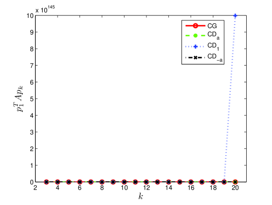
Figure 2: Conjugacy loss for an illconditioned problem described by the coefficient matrix $A_{1_{0}}$ in MN00 , using the CG, $CD_{a}$ (the $CD$ class setting $\gamma_{0}=1$ and $\gamma_{k}=a_{k}$, $k\geq 1$), $CD_{1}$ (the $CD$ class setting $\gamma_{k}=1$, $k\geq 0$) and $CD_{-a}$ (the $CD$ class setting $\gamma_{0}=1$ and $\gamma_{k}=-a_{k}$, $k\geq 1$). The quantity $p_{1}^{T}Ap_{k}$ is reported for $k\geq 3$. As evident, the choice $\gamma_{k}=1$, $k\geq 0$, can yield very harmful results when the coefficient matrix is illconditioned

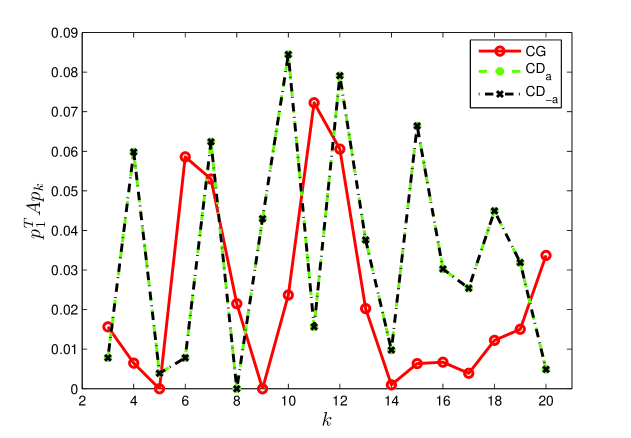
Figure 3: Conjugacy loss for an illconditioned problem described by the coefficient matrix $A_{1_{0}}$ in MN00 , using only the CG, $CD_{a}$ (the $CD$ class setting $\gamma_{0}=1$ and $\gamma_{k}=a_{k}$, $k\geq 1$) and $CD_{-a}$ (the $CD$ class setting $\gamma_{0}=1$ and $\gamma_{k}=-a_{k}$, $k\geq 1$). The quantity $p_{1}^{T}Ap_{k}$ is reported for $k\geq 3$. The choices $\gamma_{k}=a_{k}$ and $\gamma_{k}=-a_{k}$ are definitely comparable, and are preferable to the CG for $k\in\{3,6,8,11,20\}$.

We have investigated a novel class of CG-based iterative methods. This allowed us to recast several properties of the CG within a broad framework of iterative methods, based on generating mutually conjugate directions. Both the analytical properties and the geometric insight where fruitfully exploited, showing that general CG-based methods, including the CG and the scaled-CG, may be introduced. Our resulting parameter dependent CG-based framework has the distinguishing feature of including conjugacy in a more general fashion, so that numerical results may strongly rely on the choice of a set of parameters. We urge to recall that in principle, since conjugacy can be generalized to the case of $A$ indefinite (see for instance H80 ; F05 ; FaRo07 ; F05a ) potentially further generalizations with respect to $CD$ can be conceived (allowing the matrix $A$ in (1) to be possibly indefinite).
Our study and the present conclusions are not primarily inspired by the aim of possibly beating the performance of the CG on practical cases. On the contrary, we preferred to justify our proposal in the light of a general analysis, which in case (but not necessary) may suggest competitive new iterative algorithms, for solving positive definite linear systems. In a future work we are committed to consider the following couple of issues:

1. assessing clear rules for the choice of the sequence $\{\gamma_{k}\}$ in $CD$;

2. performing an extensive numerical experience, where different choices of the parameters $\{\gamma_{k}\}$ in our framework are considered, and practical guidelines for new efficient methods might be investigated.

The theory in Sects. 5 - 9 seems to provide yet premature criteria, for a fruitful choice of the sequence $\{\gamma_{k}\}$ on applications. Furthermore, we do not have clear ideas about the real importance of the scheme $CD$-red in Table 3, where the choice (28) is privileged. Anyway, to suggest the reader some numerical clues about our proposal, consider that the apparently simplest choice $\gamma_{k}=1$, $k\geq 0$, proved to be much inefficient in practice, while the choices $\gamma_{k}=\pm a_{k}$ gave appreciable results on different test problems (but still unclear results on larger test sets).

In particular we preliminarily tested the $CD$ class on two (small but) illconditioned problems described in Section 4 of MN00 . The first problem, whose coefficient matrix is addressed as $A_{1_{0}}\in\mathbb{R}^{50\times 50}$, is ‘obtained from a one-dimensional model, consisting of a line of two-node elements with support conditions at both ends and a linearly varying body force’. The second problem has the coefficient matrix $A_{2_{0}}\in\mathbb{R}^{170\times 170}$, which is ‘the stiffness matrix from a two-dimensional finite element model of a cantilever beam’.
In Figures 2-3 we report the resulting experience on just the first of the two problems (similar results hold for the other one), where the CG is compared with algorithms in the class $CD$, setting $\gamma_{k}\in\{a_{k},1,-a_{k}\}$. As a partial justification for the reported numerical experience, we note that in the $CD$ class the coefficient $\sigma_{k}$ depends on the quantity $\|Ap_{k}\|^{2}$. Thus, $\|Ap_{k}\|^{2}$ may be large when $A$ is illconditioned, so that the choice $\gamma_{k}=1$ possibly is inadequate to compensate the effect of illconditioning. On the other hand, setting $\gamma_{k}=\pm a$ and considering the expression of $a_{k}$, the coefficient $\sigma_{k}$ is possibly re-scaled, taking into account the condition number of matrix $A$.

Observe that the algorithms in $CD$ are slightly more expensive than the CG, and they require the storage of one further vector with respect to the CG. However, we proved for $CD$ some theoretical properties, which extend those provided by the CG, in order to possibly prevent from conjugacy loss. In addition, when specific values of the parameters in $CD$ are chosen, then we obtain schemes equivalent to both the CG and the scaled-CG.
Furthermore, we have also introduced preconditioning in our proposal, as a possible extension of the preconditioned CG, so that illconditioned linear systems might be possibly more efficiently tackled. Our methods are also aimed to provide an effective tool in optimization contexts where a sequence of conjugate directions is sought. Truncated Newton methods are just an example of such contexts from unconstrained nonlinear optimization, as detailed in Sect. 3. We are considering in a further study a numerical experience, over convex optimization problems, where $CD$ and the relative preconditioned scheme are adopted to solve Newton’s equation. Indeed, in case the matrix $A$ in (1) is indefinite, the choices $\gamma_{k}\in\{a_{k},|a_{k}|,-a_{k},-|a_{k}|\}$ are of some interest and might be compared on a significant test set.

In addition, it might be worth also to investigate the choice where the preconditioner ${\cal M}$ in Table 6 is computed by a Quasi-Newton approximation of the inverse matrix $A^{-1}$ (see also MN00 ; Gratton:09 ), or by using the conjugate directions generated by $CD$, for a suitable choice of the parameters (see also FaRo13 ).

Furthermore, observe that conditions (8) or (7) cannot be further generalized imposing explicitly relations ($\ell\geq 1$)

$$p_{k}^{T}Ap_{j}=0,\qquad j=k-1,k-2,\ldots,k-\ell,$$

since (8) and (7) automatically imply $p_{k}^{T}Ap_{j}=0$, for any $j\leq k-3$ (see also Lemma 1 and Lemma 2).

Finally, note that for the minimization of a convex quadratic functional in $\mathbb{R}^{n}$, the complete relation between the search directions generated by BFGS or L-BFGS updates and the CG was studied (see also NW00 ). Thus, we think that possible extensions may be considered by replacing the CG with the algorithms in our framework. In this regard, recalling that polarity (see H80 ) plays a keynote role for generating conjugate directions, there is the chance that a possible relation between the BFGS update and $CD$ could spot some light on the role of polarity for Quasi-Newton schemes.

References

(1)
Axelsson, O.: Iterative Solution Methods, Cambridge
University Press, (1996)
(2)
Golub, G.H. and Van Loan, C.F.: Matrix
computations - 3rd edition, The John Hopkins University Press, (1996)
(3)
Saad, Y.: Iterative Methods for Sparse Linear Systems,
Second Edition, SIAM, PA, (2003)
(4)
Higham, N.J.: Accuracy and Stability of Numerical
Algorithms , SIAM, PA, (1996)
(5)
Saad, Y. and Van Der Vorst, H.A.: Iterative
Solution of Linear Systems in the 20th Century, Journal on
Computational and Applied Mathematics, Vol. 123, pp. 1–33, (2000)
(6)
Greenbaum, A. and Strakos, Z.: Predicting the
Behavior of Finite Precision Lanczos and Conjugate Gradient
Computations, SIAM Journal on Matrix Analysis and Applications, Vol. 13, pp. 121–137,
(1992)
(7)
Greenbaum, A.: Iterative Methods for Solving Linear
Systems SIAM, PA, (1997)
(8)
Hestenes, M.R.: Conjugate Direction Methods in Optimization, Springer Verlag, New York, Heidelberg, Berlin, (1980)
(9)
Nash, S.G.: A survey of truncated-Newton methods,
Journal of Computational and Applied Mathematics, Vol. 124, pp.
45–59, (2000)
(10)
Conn, A.R., Gould, N.I.M. and Toint, Ph.L.: Trust region methods, MPS–SIAM Series on Optimization,
Philadelphia, PA, (2000)
(11)
Fasano, G.: Planar-Conjugate Gradient algorithm for
Large Scale Unconstrained Optimization, Part 2: Application,
Journal of Optimization Theory and Applications, Vol. 125, pp.
523–541, (2005)
(12)
Grippo, L., Lampariello, F. and Lucidi, S.: A truncated Newton method with nonmonotone linesearch for unconstrained optimization, Journal of Optimization Theory and Applications, Vol. 60, pp. 401–419, (1989)
(13)
Morales, J.L. and Nocedal, J.: Automatic
preconditioning by limited memory quasi–Newton updating, SIAM
Journal on Optimization, Vol. 10, pp. 1079–1096, (2000)
(14)
Hestenes, M.R. and Stiefel, E.: Methods of conjugate gradients for solving linear systems, Journal of Research of the National Bureau of Standards, Vol. 49, pp. 409–435, (1952)
(15)
Fasano, G.: Lanczos Conjugate-Gradient Method and
Pseudoinverse Computation on Indefinite and Singular Systems,
Journal of Optimization Theory and Applications, Vol. 132, pp.
267–285, (2007)
(16)
Stoer, J.: Solution of large linear systems of
equations by conjugate gradient type methods, In A. Bachem,
M.Grötschel, and B. Korte, editors, Mathematical Programming.
The State of the Art, pp. 540– 565, Berlin Heidelberg,
Springer-Verlag, (1983)
(17)
Nash, S.G. and Sofer, A.: Assessing a search
direction within a truncated Newton method, Operations Research Letters, Vol.
9, pp. 219–221, (1990)
(18)
Fasano, G. and Roma, M.: Iterative Computation of
Negative Curvature Directions in Large Scale Optimization,
Computational Optimization and Applications, Vol. 38, pp. 81–104,
(2007)
(19)
Gould, N.I.M., Lucidi, S., Roma, M. and Toint, Ph.L.: Exploiting negative curvature directions in linesearch methods for unconstrained optimization, Optimization Methods and Software, Vol. 14, pp. 75–98, (2000)
(20)
Fasano, G. and Lucidi, S.: A nonmonotone
truncated Newton-Krylov method exploiting negative curvature
directions, for large scale unconstrained optimization,
Optimization Letters, Vol. 3, pp. 521–535, (2009)
(21)
Nocedal, J. and Wright, S.: Numerical Optimization - 2nd edition,
Springer Series in Operations Research and Financial Engineering,
Springer, NY, (2006)
(22)
Meurant, G.: The Lanczos and Conjugate Gradient
Algorithms - from theory to finite precision computations, SIAM,
Philadelphia, USA, (2006)
(23)
Polyak, T.B.: Introduction to Optimization, Translation Series in Mathematics and Engineering, Optimization Software, Inc., Publications Division, NY, (1987)
(24)
Campbell, S.L. and Meyer JR., C.D.: Generalized Inverses of Linear Transformations,
Dover Publications, New York, NY, (1979)
(25)
Fasano, G.: Planar-Conjugate Gradient algorithm for
Large Scale Unconstrained Optimization, Part 1: Theory,
Journal of Optimization Theory and Applications, Vol. 125, pp.
543–558, (2005)
(26)
Gratton, S., Sartenaer, A. and Tshimanga, J.: On a class of limited memory preconditioners for large scale linear systems with multiple right-hand sides, SIAM Journal on Optimization, Vol. 21, pp. 912–935, (2011)
(27)
Fasano, G. and Roma, M.: Preconditioning Newton–Krylov Methods in Non-Convex Large Scale Optimization, Computational Optimization and Applications, Vol. 56, pp. 253–290,
(2013)