A Multigrid Method for the Ground State Solution of Bose-Einstein Condensates

Abstract

A multigrid method is proposed to compute the ground state solution of Bose-Einstein condensations by the finite element method based on the multilevel correction for eigenvalue problems and the multigrid method for linear boundary value problems. In this scheme, obtaining the optimal approximation for the ground state solution of Bose-Einstein condensates includes a sequence of solutions of the linear boundary value problems by the multigrid method on the multilevel meshes and a series of solutions of nonlinear eigenvalue problems on the coarsest finite element space. The total computational work of this scheme can reach almost the optimal order as same as solving the corresponding linear boundary value problem. Therefore, this type of multigrid scheme can improve the overall efficiency for the simulation of Bose-Einstein condensations. Some numerical experiments are provided to validate the efficiency of the proposed method. Keywords. BEC, GPE, eigenvalue problem, multigrid, multilevel correction, finite element method. AMS subject classifications. 65N30, 65N25, 65L15, 65B99.

1 Introduction

Recently, Bose-Einstein condensation (BEC), which is a gas of bosons that are in the same quantum state, is an active field [6, 21, 27]. In 2001, the Nobel Prize in Physics was awarded Eric A. Cornell, Wolfgang Ketterle and Carl E. Wieman [4, 17, 27] for their research in BEC. The properties of the condensate at zero or very low temperature [18, 29] can be described by the well-known Gross-Pitaevskii equation (GPE) [22, 26] which is a time-independent nonlinear Schrödinger equation [28]. So far, it is found that the GPE fits well for the most of experiments [5, 16, 18, 24].

As we know that the wave function $\psi$ of a sufficiently dilute condensates satisfies the following GPE

$$\left(-\frac{\hbar^{2}}{2m}\Delta+\widetilde{W}+\frac{4\pi\hbar^{2}aN}{m}|\psi|^{2}\right)\psi = \mu\psi,$$ (1.1)

where $\widetilde{W}$ is the external potential, $\mu$ is the chemical potential and $N$ is the number of atoms in the condensate. The effective two-body interaction is $4\pi\hbar^{2}a/m$, where $\hbar$ is the Plank constant, $a$ is the scattering length (positive for repulsive interaction and negative for attractive interaction) and $m$ is the particle mass. In this paper, we assume the external potential $\widetilde{W}(x)$ is measurable and locally bounded and tends to infinity as $|x|\rightarrow\infty$ in the sense that

$$\inf_{|x|\geq r}\widetilde{W}(x)\rightarrow\infty\ \ \ \ {\rm for}\ r\rightarrow\infty.$$

Then the wave function $\psi$ must vanish exponentially fast as $|x|\rightarrow\infty$. Furthermore (1.1) can be written as

$$\left(-\Delta+\frac{2m}{\hbar^{2}}\widetilde{W}+8\pi aN|\psi|^{2}\right)\psi = \frac{2m\mu}{\hbar^{2}}\psi.$$ (1.2)

Hence in this paper, we are concerned with the following non-dimensionalized GPE problem:
Find $(\lambda,u)\in\mathbb{R}\times H_{0}^{1}(\Omega)$ such that

$$\left\{\begin{array}[]{rcl}-\Delta u+Wu+\zeta|u|^{2}u&=&\lambda u,\ \ \ {\rm in}\ \Omega,\\ u&=&0,\ \ \ \ \ {\rm on}\ \partial\Omega,\\ \int_{\Omega}|u|^{2}&=&1,\end{array}\right.$$ (1.3)

where $\Omega\subset\mathbb{R}^{d}$ $(d=1,2,3)$ denotes the computing domain which have the cone property [1], $\zeta$ is some positive constant and $W(x)=\gamma_{1}x^{2}_{1}+\cdots+\gamma_{d}x^{2}_{d}\geq 0$ with $\gamma_{1},\cdots,\gamma_{d}>0$ [8, 37].

So far, there have existed many papers discussing the numerical methods for the time-dependent GPEs and time-independent GPEs. Please refer to the papers [2, 3, 5, 6, 7, 8, 13, 14, 16, 17, 18, 19, 20, 27, 32] and the papers cited therein. Especially, in [37], the convergence of the finite element method for GPEs has been proved and the priori error estimates of the finite element method for GPEs has been presented in [12] which will be used in this paper.

Recently, a type of multigrid method for eigenvalue problems has been proposed in [30, 33, 34, 35]. The aim of this paper is to present a multigrid scheme for GPE (1.3) based on the multilevel correction method in [30]. With this method, solving GPE will not be more difficult than solving the corresponding linear boundary value problem. The multigrid method for GPE is based on a series of nested finite element spaces with different level of accuracy which can be built in the same way as the multilevel method for boundary value problems [36]. The corresponding error and computational work estimates of the proposed multigrid scheme for the GPE will also be analyzed. Based on the analysis, the proposed method can obtain optimal errors with an almost optimal computational work. The eigenvalue multigrid procedure can be described as follows: (1) solve the GPE in the initial finite element space; (2) use the multigrid method to solve an additional linear boundary value problem which is constructed by using the previous obtained eigenpair approximation; (3) solve a GPE again on the finite element space which is constructed by combining the coarsest finite element space with the obtained eigenfunction approximation in step (2). Then go to step (2) for the next loop until stop. In this method, we replace solving semi-linear eigenvalue problem GPE on the finest finite element space by solving a series of linear boundary value problems with multigrid scheme in the corresponding series of finite element spaces and a series of GPEs in the coarsest finite element space. So this multigrid method can improve the overall efficiency of solving GPEs as it does for linear boundary value problems.

An outline of the paper goes as follows. In Section 2, we introduce finite element method for the ground state solution of BEC, i.e. non-dimensionalized GPE (1.3). A type of one corrections step is given in Sections 3 based on the fixed-point iteration. In Section 4, we propose a type of multigrid algorithm for solving the non-dimensionalized GPE by the finite element method. Section 5 is devoted to estimating the computational work for the multigrid method defined in Section 4. Two numerical examples are provided in Section 6 to validate our theoretical analysis. Some concluding remarks are given in the last section.

2 Finite element method for GPE problem

In this section, we introduce some notation and the finite element method for GPE (1.3). The letter $C$ (with or without subscripts) denotes a generic positive constant which may be different at its different occurrences. For convenience, the symbols $\lesssim$, $\gtrsim$ and $\approx$ will be used in this paper. That $x_{1}\lesssim y_{1},x_{2}\gtrsim y_{2}$ and $x_{3}\approx y_{3}$, mean that $x_{1}\leq C_{1}y_{1}$, $x_{2}\geq c_{2}y_{2}$ and $c_{3}x_{3}\leq y_{3}\leq C_{3}x_{3}$ for some constants $C_{1},c_{2},c_{3}$ and $C_{3}$ that are independent of mesh sizes (see, e.g., [36]). We shall use the standard notation for Sobolev spaces $W^{s,p}(\Omega)$ and their associated norms $\|\cdot\|_{s,p,\Omega}$ and seminorms $|\cdot|_{s,p,\Omega}$ (see, e.g., [1]). For $p=2$, we denote $H^{s}(\Omega)=W^{s,2}(\Omega)$ and $H_{0}^{1}(\Omega)=\{v\in H^{1}(\Omega):\ v|_{\partial\Omega}=0\}$, where $v|_{\partial\Omega}=0$ is in the sense of trace, $\|\cdot\|_{s,\Omega}=\|\cdot\|_{s,2,\Omega}$. In this paper, we set $V=H_{0}^{1}(\Omega)$. and use $\|\cdot\|_{s}$ to denote $\|\cdot\|_{s,\Omega}$ for simplicity.

For the aim of finite element discretization, we define the corresponding weak form for (1.3) as follows:
Find $(\lambda,u)\in\mathbb{R}\times V$ such that $b(u,u)=1$ and

$$a(u,v)=\lambda b(u,v),\ \ \ \forall v\in V,$$ (2.1)

where

$$a(u,v):=\int_{\Omega}\big{(}\nabla u\nabla v+Wuv+\zeta|u|^{2}uv\big{)}d\Omega,\ \ \ \ b(u,v):=\int_{\Omega}uvd\Omega.$$

Now, let us define the finite element method [11, 15] for the problem (2.1). First we generate a shape-regular decomposition of the computing domain $\Omega\subset\mathbb{R}^{d}$ $(d=2,3)$ into triangles or rectangles for $d=2$ (tetrahedrons or hexahedrons for $d=3$) and the diameter of a cell $K\in\mathcal{T}_{h}$ is denoted by $h_{K}$. The mesh diameter $h$ describes the maximum diameter of all cells $K\in\mathcal{T}_{h}$. Based on the mesh $\mathcal{T}_{h}$, we construct the linear finite element space denoted by $V_{h}\subset V$. We assume that $V_{h}\subset V$ is a family of finite-dimensional spaces that satisfy the following assumption:

$$\lim_{h\rightarrow 0}\inf_{v\in V_{h}}\|w-v\|_{1}=0,\ \ \ \forall w\in V.$$ (2.2)

The standard finite element method for (2.1) is to solve the following eigenvalue problem:
Find $(\bar{\lambda}_{h},\bar{u}_{h})\in\mathbb{R}\times V_{h}$ such that $b(\bar{u}_{h},\bar{u}_{h})=1$ and

$$a(\bar{u}_{h},v_{h})=\bar{\lambda}_{h}b(\bar{u}_{h},v_{h}),\ \ \ \forall v_{h}\in V_{h}.$$ (2.3)

Then we define

$$\delta_{h}(u):=\inf_{v_{h}\in V_{h}}\|u-v_{h}\|_{1}.$$ (2.4)

Lemma 2.1.

([12, Theorem 1]) There exists $h_{0}>0$, such that for all $0<h<h_{0}$, the smallest eigenpair approximation $(\bar{\lambda}_{h},\bar{u}_{h})$ of (2.3) having the following error estimates

$$\|u-\bar{u}_{h}\|_{1} \lesssim \delta_{h}(u),$$ (2.5)

$$\|u-\bar{u}_{h}\|_{0} \lesssim \eta_{a}(V_{h})\|u-\bar{u}_{h}\|_{1}\lesssim\eta_{a}(V_{h})\delta_{h}(u),$$ (2.6)

$$|\lambda-\bar{\lambda}_{h}| \lesssim \|u-\bar{u}_{h}\|^{2}_{1}+\|u-\bar{u}_{h}\|_{0}\lesssim\eta_{a}(V_{h})\delta_{h}(u),$$ (2.7)

where $\eta_{a}(V_{h})$ is defined as follows

$$\eta_{a}(V_{h})=\|u-\bar{u}_{h}\|_{1}+\sup_{f\in L^{2}(\Omega),\|f\|_{0}=1}\inf_{v_{h}\in V_{h}}\|Tf-v_{h}\|_{1}$$ (2.8)

with the operator $T$ being defined as follows:
Find $Tf\in u^{\perp}$ such that

$$a(Tf,v)+2(\zeta|u|^{2}(Tf),v)-(\lambda(Tf),v)=(f,v),\ \ \ \ \forall v\in u^{\perp},$$

and $u^{\perp}=\big{\{}v\in H_{0}^{1}(\Omega):|\int_{\Omega}uvd\Omega=0\big{\}}$.

3 One correction step based on fixed-point iteration

In this section, we introduce a type of one correction step based on the fixed-point iteration to improve the accuracy of the given eigenpair approximation. This correction step contains solving an auxiliary linear boundary value problem with multigrid method in the finer finite element space and a GPE on the coarsest finite element space.

In order to define the one correction step, we introduce a very coarse mesh $\mathcal{T}_{H}$ and the low dimensional linear finite element space $V_{H}$ defined on the mesh $\mathcal{T}_{H}$. Assume we have obtained an eigenpair approximation $(\lambda_{h_{k}},u_{h_{k}})\in\mathbb{R}\times V_{h_{k}}$ and the coarse space $V_{H}$ is a subset of $V_{h_{k}}$. Now we introduce a type of one correction step to improve the accuracy of the given eigenpair approximation $(\lambda_{h_{k}},u_{h_{k}})$. Let $V_{h_{k+1}}\subset V$ be a finer finite element space of $V_{h_{k}}$ such that $V_{h_{k}}\subset V_{h_{k+1}}$. Based on this finer finite element space, we define the following one correction step.

Algorithm 3.1.

One Correction Step based on Fixed-point Iteration

1. Define the following auxiliary boundary value problem:
   Find $\widehat{e}_{h_{k+1}}\in V_{h_{k+1}}$ such that

   $$(\nabla\widehat{e}_{h_{k+1}},\nabla v_{h_{k+1}})=\lambda_{h_{k}}b(u_{h_{k}},v_{h_{k+1}})-a(u_{h_{k}},v_{h_{k+1}}),\ \ \ \forall v_{h_{k+1}}\in V_{h_{k+1}}.$$ (3.1)

   Solve this equation with multigrid method [9, 11, 23, 31, 36] to obtain an approximation $\widetilde{e}_{h_{k+1}}\in V_{h_{k+1}}$ with the error estimate $\|\widetilde{e}_{h_{k+1}}-\widehat{e}_{h_{k+1}}\|_{1}\lesssim\varsigma_{h_{k+1}}$ and set $\widetilde{u}_{h_{k+1}}=u_{h_{k}}+\widetilde{e}_{h_{k+1}}$. Here $\varsigma_{h_{k+1}}$ is used to denote the accuracy for the multigrid iteration.

2. Define a new finite element space $V_{H,h_{k+1}}=V_{H}+{\rm span}\{\widetilde{u}_{h_{k+1}}\}$ and solve the following eigenvalue problem:
   Find $(\lambda_{h_{k+1}},u_{h_{k+1}})\in\mathbb{R}\times V_{H,h_{k+1}}$ such that $b(u_{h_{k+1}},u_{h_{k+1}})=1$ and

   $$a(u_{h_{k+1}},v_{H,h_{k+1}})=\lambda_{h_{k+1}}b(u_{h_{k+1}},v_{H,h_{k+1}}),\ \ \forall v_{H,h_{k+1}}\in V_{H,h_{k+1}}.$$ (3.2)

Summarize above two steps into

$$(\lambda_{h_{k+1}},u_{h_{k+1}})=Correction(V_{H},\lambda_{h_{k}},u_{h_{k}},V_{h_{k+1}},\varsigma_{h_{k+1}}).$$

Theorem 3.1.

Assume $h_{k}<h_{0}$ and there exists a real number $\varepsilon_{h_{k}}(u)$ such that the given eigenpair approximation $(\lambda_{h_{k}},u_{h_{k}})\in\mathbb{R}\times V_{h_{k}}$ has the following error estimates

$$\|\bar{u}_{h_{k}}-u_{h_{k}}\|_{0}+|\bar{\lambda}_{h_{k}}-\lambda_{h_{k}}|=\varepsilon_{h_{k}}(u).$$ (3.3)

Then after one correction step, the resultant approximation $(\lambda_{h_{k+1}},u_{h_{k+1}})\in\mathbb{R}\times V_{h_{k+1}}$ has the following error estimates

$$\|\bar{u}_{h_{k+1}}-u_{h_{k+1}}\|_{1} \lesssim \varepsilon_{h_{k+1}}(u),$$ (3.4)

$$\|\bar{u}_{h_{k+1}}-u_{h_{k+1}}\|_{0} \lesssim \eta_{a}(V_{H})\|u-u_{h_{k+1}}\|_{1},$$ (3.5)

$$|\bar{\lambda}_{h_{k+1}}-\lambda_{h_{k+1}}| \lesssim \eta_{a}(V_{H})\varepsilon_{h_{k+1}}(u),$$ (3.6)

where $\varepsilon_{h_{k+1}}(u):=\eta_{a}(V_{h_{k}})\delta_{h_{k}}(u)+\|\bar{u}_{h_{k}}-u_{h_{k}}\|_{0}+|\bar{\lambda}_{h_{k}}-\lambda_{h_{k}}|+\varsigma_{h_{k+1}}$.

Proof.

First, we define $H^{1}(\Omega)$ inner-product $\widehat{a}(\cdot,\cdot)$ as

$$\widehat{a}(w,v)=\int_{\Omega}\nabla w\nabla vd\Omega,\ \ \ \forall w,v\in V.$$

From problems (2.3) and (3.1), inequality (3.3), Lemma 2.1, Hölder inequality and Sobolev space embedding inequality, the following estimates hold for any $v_{h_{k+1}}\in V_{h_{k+1}}$

$$\widehat{a}(\bar{u}_{h_{k+1}}-u_{h_{k}}-\widehat{e}_{h_{k+1}},v_{h_{k+1}})$$

$$= b(\bar{\lambda}_{h_{k+1}}\bar{u}_{h_{k+1}}-\lambda_{h_{k}}u_{h_{k}},v_{h_{k+1}})$$

$$+\big{(}(W+\zeta\|u_{h_{k}}\|^{2})u_{h_{k}}-(W+\zeta\|\bar{u}_{h_{k+1}}\|^{2})\bar{u}_{h_{k+1}},v_{h_{k+1}}\big{)}$$

$$\lesssim \|\bar{\lambda}_{h_{k+1}}\bar{u}_{h_{k+1}}-\lambda_{h_{k}}u_{h_{k}}\|_{0}\|v_{h_{k+1}}\|_{1}$$

$$\ \ \ +\|\bar{u}_{h_{k+1}}-u_{h_{k}}\|_{0}(\|\bar{u}_{h_{k+1}}\|_{0,6,\Omega}^{2}+\|u_{h_{k}}\|_{0,6,\Omega}^{2})\|v_{h_{k+1}}\|_{0,6,\Omega}$$

$$\lesssim \Big{(}\|\bar{\lambda}_{h_{k+1}}\bar{u}_{h_{k+1}}-\bar{\lambda}_{h_{k}}\bar{u}_{h_{k}}\|_{0}+\|\bar{\lambda}_{h_{k}}\bar{u}_{h_{k}}-\lambda_{h_{k}}u_{h_{k}}\|_{0}\big{)}\|v_{h_{k+1}}\|_{1}$$

$$\ \ \ \ +\big{(}\|\bar{u}_{h_{k+1}}-\bar{u}_{h_{k}}\|_{0}+\|\bar{u}_{h_{k}}-u_{h_{k}}\|_{0}\big{)}(\|\bar{u}_{h_{k+1}}\|_{1}^{2}+\|u_{h_{k}}\|_{1}^{2})\|v_{h_{k+1}}\|_{1}$$

$$\lesssim \big{(}\eta_{a}(V_{h_{k}})\delta_{h_{k}}(u)+\varepsilon_{h_{k}}(u)\big{)}\|v_{h_{k+1}}\|_{1}.$$

Then we have

$$\|\bar{u}_{h_{k+1}}-u_{h_{k}}-\widehat{e}_{h_{k+1}}\|_{1}\lesssim\eta_{a}(V_{h_{k}})\delta_{h_{k}}(u)+\varepsilon_{h_{k}}(u).$$ (3.7)

From (3.7) and $\|\widetilde{e}_{h_{k+1}}-\widehat{e}_{h_{k+1}}\|_{1}\lesssim\varsigma_{h_{k+1}}$, the following estimate holds

$$\|\bar{u}_{h_{k+1}}-\widetilde{u}_{h_{k+1}}\|_{1}=\|\bar{u}_{h_{k+1}}-u_{h_{k}}-\widetilde{e}_{h_{k+1}}\|_{1}\lesssim\eta_{a}(V_{h_{k}})\delta_{h_{k}}(u)+\varepsilon_{h_{k}}(u)+\varsigma_{h_{k+1}}.$$ (3.8)

Now we come to estimate the error for the eigenpair solution $(\lambda_{h_{k+1}},u_{h_{k+1}})$ of problem (3.2). Since $V_{H,h_{k+1}}$ is a subset of $V_{h_{k+1}}$, we can think of problem (3.2) as a subspace approximation for the problem (2.3). Then based on the definition of $V_{H,h_{k+1}}$, the subspace approximation result from [12] and Lemma 2.1, the following estimates hold

$$\|\bar{u}_{h_{k+1}}-u_{h_{k+1}}\|_{1} \lesssim \inf_{v_{H,h_{k+1}}\in V_{H,h_{k+1}}}\|\bar{u}_{h_{k+1}}-v_{H,h_{k+1}}\|\leq\|\bar{u}_{h_{k+1}}-\widetilde{u}_{h_{k+1}}\|_{1}$$ (3.9)

$$\lesssim \eta_{a}(V_{h_{k}})\delta_{h_{k}}(u)+\varepsilon_{h_{k}}(u)+\varsigma_{h_{k+1}}.$$

This is the desired result (3.4). Then (3.5) and (3.6) can be proved based on (3.4) and Lemma 2.1. ∎

4 Multigrid method for GPE

In this section, we introduce a type of multigrid method based on the One Correction Step defined in Algorithms 3.1. This type of multigrid method can obtain the optimal error estimate as same as solving the GPE directly on the finest finite element space.

In order to do multigrid scheme, we define a sequence of triangulations $\mathcal{T}_{h_{k}}$ of $\Omega$ determined as follows. Suppose $\mathcal{T}_{h_{1}}$ is produced from $\mathcal{T}_{H}$ by the regular refinement and let $\mathcal{T}_{h_{k}}$ be obtained from $\mathcal{T}_{h_{k-1}}$ via regular refinement such that

$$h_{k}\approx\frac{1}{\beta}h_{k-1},\ \ \ \ k=2,\cdots,n,$$

where $\beta$ denotes the refinement index. Based on this sequence of meshes, we construct the corresponding linear finite element spaces $V_{h_{1}},\cdots,V_{h_{n}}$ such that

$$V_{H}=V_{h_{0}}\subseteq V_{h_{1}}\subset V_{h_{2}}\subset\cdots\subset V_{h_{n}}\subset V.$$ (4.1)

In this paper, we assume the following relations of approximation errors hold

$$\eta_{a}(V_{h_{k}})\approx\frac{1}{\beta}\eta_{a}(V_{h_{k-1}}),\ \ \ \ \delta_{h_{k}}(u)\approx\frac{1}{\beta}\delta_{h_{k-1}}(u),\ \ \ k=2,\cdots,n.$$ (4.2)

Algorithm 4.1.

Multigrid Scheme for GPE

1. Construct a series of nested finite element spaces $V_{H},V_{h_{1}},V_{h_{2}},\cdots,V_{h_{n}}$ such that (4.1) and (4.2) hold.

2. Solve the GPE on the initial finite element space $V_{h_{1}}$:
   Find $(\lambda_{h_{1}},u_{h_{1}})\in\mathbb{R}\times V_{h_{1}}$ such that $b(u_{h_{1}},u_{h_{1}})=1$ and

   $$a(u_{h_{1}},v_{h_{1}}) = \lambda_{h_{1}}b(u_{h_{1}},v_{h_{1}}),\ \ \ \ \forall v_{h_{1}}\in V_{h_{1}}.$$

3. Do $k=1,\cdots,n-1$
   Obtain a new eigenpair approximation $(\lambda_{h_{k+1}},u_{h_{k+1}})\in\mathbb{R}\times V_{h_{k+1}}$ with the one correction step defined by Algorithm 3.1

   $$(\lambda_{h_{k+1}},u_{h_{k+1}})={\it Correction}(V_{H},\lambda_{h_{k}},u_{h_{k}},V_{h_{k+1}},\varsigma_{h_{k+1}}).$$

   end Do

Finally, we obtain an eigenpair approximation $(\lambda_{h_{n}},u_{h_{n}})\in\mathbb{R}\times V_{h_{n}}$.

Theorem 4.1.

Assume $h_{1}<h_{0}$ and the error $\varsigma_{h_{k+1}}$ of the linear solving by the multigrid method in the $k+1$-th level mesh satisfies $\varsigma_{h_{k+1}}\leq\eta_{a}(V_{h_{k}})\delta_{h_{k}}(u)$ for $k=1,\cdots,n-1$. After implementing Algorithm 4.1, the resultant eigenpair approximation $(\lambda_{h_{n}},u_{h_{n}})$ has the following error estimates

$$\|\bar{u}_{h_{n}}-u_{h_{n}}\|_{1} \lesssim \beta^{2}\eta_{a}(V_{h_{n}})\delta_{h_{n}}(u),$$ (4.3)

$$\|\bar{u}_{h_{n}}-u_{h_{n}}\|_{0} \lesssim \eta_{a}(V_{h_{n}})\delta_{h_{n}}(u),$$ (4.4)

$$|\bar{\lambda}_{h_{n}}-\lambda_{h_{n}}| \lesssim \eta_{a}(V_{h_{n}})\delta_{h_{n}}(u),$$ (4.5)

with the condition $C\beta^{2}\eta_{a}(V_{H})<1$ for the concerned constant $C$.

Proof.

From Lemma 2.1 and the definition of Algorithm 4.1, we have $\bar{u}_{h_{1}}=u_{h_{1}}$ and $\bar{\lambda}_{h_{1}}=\lambda_{h_{1}}$. Then from the proof of Theorem 3.1 with $\varepsilon_{h_{1}}(u)=0$ and $\varsigma_{h_{2}}\lesssim\eta_{a}(V_{h_{1}})\delta_{h_{1}}(u)$, the following estimates hold

$$\|\bar{u}_{h_{2}}-u_{h_{2}}\|_{1} \lesssim \eta_{a}(V_{h_{1}})\delta_{h_{1}}(u),$$ (4.6)

$$\|\bar{u}_{h_{2}}-u_{h_{2}}\|_{0} \lesssim \eta_{a}(V_{H})\|\bar{u}_{h_{2}}-u_{h_{2}}\|_{1}\lesssim\eta_{a}(V_{H})\eta_{a}(V_{h_{1}})\delta_{h_{1}}(u),$$ (4.7)

$$|\bar{\lambda}_{h_{2}}-\lambda_{h_{2}}| \lesssim \eta_{a}(V_{H})\|\bar{u}_{h_{2}}-u_{h_{2}}\|_{1}\lesssim\eta_{a}(V_{H})\eta_{a}(V_{h_{1}})\delta_{h_{1}}(u).$$ (4.8)

Based on Theorem 3.1, (4.2), (4.6)-(4.8) and recursive argument, the final eigenfunction approximation $u_{h_{n}}$ has the following error estimates

$$\|\bar{u}_{h_{n}}-u_{h_{n}}\|_{1} \lesssim \eta_{a}(V_{h_{n-1}})\delta_{h_{n-1}}(u)+\|\bar{u}_{h_{n-1}}-u_{h_{n-1}}\|_{0}+|\bar{\lambda}_{h_{n-1}}-\lambda_{h_{n-1}}|$$

$$\lesssim \eta_{a}(V_{h_{n-1}})\delta_{h_{n-1}}(u)+\eta_{a}(V_{H})\|\bar{u}_{h_{n-1}}-u_{h_{n-1}}\|_{1}$$

$$\lesssim \eta_{a}(V_{h_{n-1}})\delta_{h_{n-1}}(u)+\eta_{a}(V_{H})\eta_{a}(V_{h_{n-2}})\delta_{h_{n-2}}(u)$$

$$\ \ \ \ +\eta_{a}^{2}(V_{H})\|\bar{u}_{h_{n-2}}-u_{h_{n-2}}\|_{1}$$

$$\lesssim \sum^{n-1}_{k=1}\big{(}\eta_{a}(V_{H})\big{)}^{n-k-1}\eta_{a}(V_{h_{k}})\delta_{h_{k}}(u)$$

$$\lesssim \Big{(}\sum^{n-1}_{k=1}\big{(}\beta^{2}\eta_{a}(V_{H})\big{)}^{n-k-1}\Big{)}\beta^{2}\eta_{a}(V_{h_{n}})\delta_{h_{n}}(u)$$

$$\lesssim \frac{1}{1-\beta^{2}\eta_{a}(V_{H})}\beta^{2}\eta_{a}(V_{h_{n}})\delta_{h_{n}}(u)\lesssim\beta^{2}\eta_{a}(V_{h_{n}})\delta_{h_{n}}(u).$$

This means we have obtained the desired result (4.3). And (4.4) can be proved by the similar argument in the proof for Theorem 3.1 which can be stated as follows

$$\|\bar{u}_{h_{n}}-u_{h_{n}}\|_{0}\lesssim\eta_{a}(V_{H})\|\bar{u}_{h_{n}}-u_{h_{n}}\|_{1}\lesssim\eta_{a}(V_{H})\beta^{2}\eta_{a}(V_{h_{n}})\delta_{h_{n}}(u)\leq\eta_{a}(V_{h_{n}})\delta_{h_{n}}(u).$$

Similar derivative can lead to the desired result (4.5) and the proof is complete. ∎

Based on the results in Theorem 4.1, we can give the final error estimates for Algorithm 4.1 as follows.

Corollary 4.1.

Under the conditions of Theorem 4.1, we have the following error estimates

$$\|u-u_{h_{n}}\|_{1} \lesssim \delta_{h_{n}}(u),$$ (4.9)

$$\|u-u_{h_{n}}\|_{0} \lesssim \eta_{a}(V_{h_{n}})\delta_{h_{n}}(u),$$ (4.10)

$$|\lambda-\lambda_{h_{n}}| \lesssim \eta_{a}(V_{h_{n}})\delta_{h_{n}}(u).$$ (4.11)

5 Discussion of the computational work

In this section, we come to analyze the computational work for the multigrid scheme defined in Algorithm 4.1. Since the linear boundary value problem (3.1) in Algorithm 3.1 is solved by multigrid method, the computational work for this part is optimal order.

First, we define the dimension of each level linear finite element space as

$$N_{k}:={\rm dim}V_{h_{k}},\ \ \ k=1,\cdots,n.$$

Then we have

$$N_{k}\thickapprox\Big{(}\frac{1}{\beta}\Big{)}^{d(n-k)}N_{n},\ \ \ k=1,\cdots,n.$$ (5.1)

The computational work for the second step in Algorithm 3.1 is different from the linear eigenvalue problems [30, 33, 34, 35]. In this step, we need to solve a nonlinear eigenvalue problem (3.2). Always, some type of nonlinear iteration method (self-consistent iteration or Newton type iteration) is used to solve this nonlinear eigenvalue problem. In each nonlinear iteration step, we need to build the matrix on the finite element space $V_{H,h_{k}}$ ($k=2,\cdots,n$) which needs the computational work $\mathcal{O}(N_{k})$. Fortunately, the matrix building can be carried out by the parallel way easily in the finite element space since it has no data transfer.

Theorem 5.1.

Assume we use $m$ computing-nodes in Algorithm 4.1, the GPE problem solved in the coarse spaces $V_{H,h_{k}}$ ($k=1,\cdots,n$) and $V_{h_{1}}$ need work $\mathcal{O}(M_{H})$ and $\mathcal{O}(M_{h_{1}})$, respectively, and the work multigrid method for solving the source problem in $V_{h_{k}}$ be $\mathcal{O}(N_{k})$ for $k=2,3,\cdots,n$. Let $\varpi$ denote the nonlinear iteration times when we solve the nonlinear eigenvalue problem (3.2). Then in each computational node, the work involved in Algorithm 4.1 has the following estimate

$${\rm Total\ work} = \mathcal{O}\Big{(}\big{(}1+\frac{\varpi}{m}\big{)}N_{n}+M_{H}\log N_{n}+M_{h_{1}}\Big{)}.$$ (5.2)

Proof.

Let $W_{k}$ denote the work in any processor of the correction step in the $k$-th finite element space $V_{h_{k}}$. Then with the correction definition, we have

$$W_{k} = \mathcal{O}\left(N_{k}+M_{H}+\varpi\frac{N_{k}}{m}\right).$$ (5.3)

Iterating (5.3) and using the fact (5.1), we obtain

Total work $$= \sum_{k=1}^{n}W_{k}=\mathcal{O}\left(M_{h_{1}}+\sum_{k=2}^{n}\Big{(}N_{k}+M_{H}+\varpi\frac{N_{k}}{m}\Big{)}\right)$$ (5.4)

$$= \mathcal{O}\Big{(}\sum_{k=2}^{n}\Big{(}1+\frac{\varpi}{m}\Big{)}N_{k}+(n-1)M_{H}+M_{h_{1}}\Big{)}$$

$$= \mathcal{O}\left(\sum_{k=2}^{n}\Big{(}\frac{1}{\beta}\Big{)}^{d(n-k)}\Big{(}1+\frac{\varpi}{m}\Big{)}N_{n}+M_{H}\log N_{n}+M_{h_{1}}\right)$$

$$= \mathcal{O}\left(\big{(}1+\frac{\varpi}{m}\big{)}N_{n}+M_{H}\log N_{n}+M_{h_{1}}\right).$$

This is the desired result and we complete the proof. ∎

Remark 5.1.

Since we have a good enough initial solution $\widetilde{u}_{h_{k+1}}$ in the second step of Algorithm 3.1, then solving the nonlinear eigenvalue problem (3.2) always does not need many nonlinear iteration times (always $\varpi\leq 3$). In this case, the complexity in each computational node will be $\mathcal{O}(N_{n})$ provided $M_{H}\ll N_{n}$ and $M_{h_{1}}\leq N_{n}$.

6 Numerical examples

In this section, we provided two numerical examples to validate the efficiency of the multigrid method stated in Algorithm 4.1.

Example 6.1.

In this example, we solve GPE (1.1) with the computing domain $\Omega$ being the unit square $\Omega=(0,1)\times(0,1)$, $W=x_{1}^{2}+x_{2}^{2}$ and $\zeta=1$.

The sequence of finite element spaces are constructed by using the linear finite element on the series of meshes which are produced by regular refinement with $\beta=2$ (connecting the midpoints of each edge). In this example, we use two meshes which are generated by Delaunay method as the initial mesh $\mathcal{T}_{H}=\mathcal{T}_{h_{1}}$ to investigate the convergence behaviors. Since the exact eigenvalue is not known, we choose an adequately accurate approximation as the exact first eigenvalue for our numerical tests. Figure 1 shows the corresponding initial meshes: one is coarse and the other is fine.

From the error estimate result of GPEs by the finite element method, we have

$$\delta_{h}(u)=h,\ \ \ \ \ \eta_{a}(V_{h})=h.$$

Then from Theorem 4.1, the following estimates hold

$$\|\bar{u}_{h_{n}}-u_{h_{n}}\|_{1}\lesssim h_{n}^{2},\ \ \ \ \|\bar{u}_{h_{n}}-u_{h_{n}}\|_{0}\lesssim h_{n}^{2},\ \ \ \ |\bar{\lambda}_{h_{n}}-\lambda_{h_{n}}|\lesssim h_{n}^{2}.$$ (6.1)

Algorithm 4.1 is applied to solve the GPE. For comparison, we also solve the GPE directly by the finite element method. Figure 2 gives the corresponding numerical results for the ground state solution (the smallest eigenvalue and the corresponding eigenfunction) corresponding to the two initial meshes illustrated in Figure 1. From Figure 2, we find the multigrid scheme can obtain the optimal error estimates as same as the direct finite element method for the eigenvalue and the corresponding eigenfunction approximations which validates the results stated in Theorem 4.1 and (6.1).

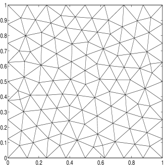
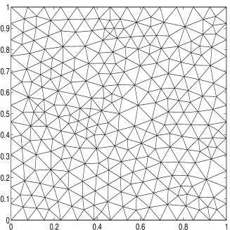
Figure 1: The coarse and fine initial meshes for the unit square (left: $H=1/6$ and right: $H=1/12$)

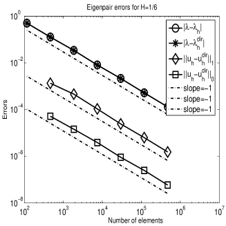
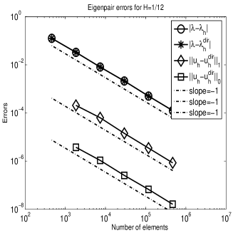
Figure 2: The errors of the multigrid algorithm for the first eigenvalue and the corresponding eigenfunction, where $u_{h}^{\rm dir}$ and $\lambda_{h}^{\rm dir}$ denote the eigenfunction and eigenvalue approximation by direct eigenvalue solving (The left figure corresponds to the left mesh in Figure 1 and the right figure corresponds to the right right mesh in Figure 1)

Example 6.2.

In this example, we also solve the GPE (1.1), where the computing domain $\Omega$ is the $L$-shape domain $\Omega=(-1,1)\times(-1,1)\backslash[0,1)\times(-1,0]$, $W=x_{1}^{2}+x_{2}^{2}$ and $\zeta=1$.

Since $\Omega$ has a reentrant corner, eigenfunctions with singularities are expected. The convergence order for eigenvalue approximations is less than $2$ by the linear finite element method which is the order predicted by the theory for regular eigenfunctions. Thus, the adaptive refinement is adopted to couple with the multigrid method described in Algorithm 4.1 and the ZZ-method [38] is used to compute the a posteriori error estimators.

First, we investigate the numerical results for the first eigenvalue approximations. Since the exact eigenvalue is not known, we also choose an adequately accurate approximation as the exact smallest eigenvalue for our numerical tests. We give the numerical results of the multigrid method in which the sequence of meshes $\mathcal{T}_{h_{1}}$, $\cdots$, $\mathcal{T}_{h_{n}}$ is produced by the adaptive refinement. Figure 3 shows the mesh after $15$ adaptive iterations and the corresponding numerical results for the adaptive iterations. From Figure 3, we can find the multigrid method can also work on the adaptive family of meshes and obtain the optimal accuracy. The multigrid method can be coupled with the adaptive refinement naturally which produce a type of adaptive finite element method (AFEM) for the GPE where the direct eigenvalue solving in the finest space is not required. This can also improve the overall efficiency of the AFEM for the nonlinear eigenvalue problem solving.

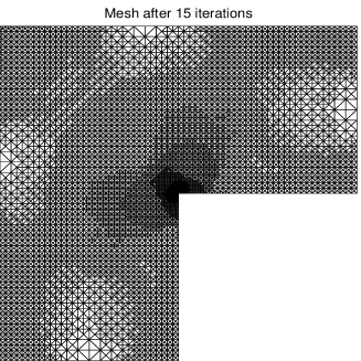
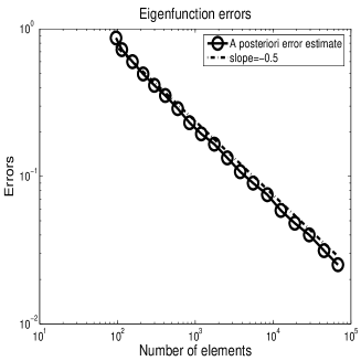
Figure 3: The triangulations after adaptive iterations for Example 6.2 by the linear element (left) and the posteriori error estimates for the eigenfunction approximations (right)

7 Concluding remarks

In this paper, we propose a multigrid method to solve the GPE based on the multilevel correction method. With this method, solving GPE is not more difficult than solving the corresponding linear boundary value problem. The corresponding error and computational work estimate have also been given for the proposed multigrid scheme. The idea and the method here can also be extended to other nonlinear eigenvalue problems which always comes from the electronic structure computation. Algorithm 4.1 can also be coupled with other numerical schemes to produce some efficient solvers for nonlinear eigenvalue problems.

References

- [1] R. A. Adams, Sobolev spaces, Academic Press, New York, 1975.
- [2] S. K. Adhikari, Collapse of attractive Bose-Einstein condensed vortex states in a cylindrical trap, Phys. Rev. E, 65 (2002), 016703.
- [3] S. K. Adhikari, P. Muruganandam, Bose-Einstein condensation dynamics from the numerical solution of the Gross-Pitaevskii equation, J. Phys. B, 35 (2002), 2831.
- [4] M. H. Anderson, J. R. Ensher , M. R. Mattews , C. E. Wieman and E. A. Cornell, Observation of Bose-Einstein condensation in a dilute atomic vapor, Science, 269 (1995), 198-201.
- [5] J. R. Anglin and W. Ketterle, Bose-Einstein condensation of atomic gasses, Nature, 416 (2002), 211-218
- [6] W. Bao and Y. Cai, Mathematical theory and numerical methods for Bose-Einstein condestion, Kinetic and Related Models, 6(1) (2013), 1-135.
- [7] W. Bao and Q. Du, Computing the ground state solution of Bose-Einstein condensates by a normalized gradient flow, Siam J. Sci. Comput., 25(5) (2004), 1674-1697.
- [8] W. Bao and W. Tang, Ground-state solution of trapped interacting Bose-Einstein condensate by directly minimizing the energy functional, J. Comput. Phys., 187 (2003), 230-254.
- [9] J. H. Bramble, Multigrid Methods, Pitman Research Notes in Mathematics, V. 294, John Wiley and Sons, 1993.
- [10] J. H. Bramble and J. E. Pasciak, New convergence estimates for multigrid algorithms, Math. Comp., 49 (1987), 311-329.
- [11] S. Brenner and L. Scott, The Mathematical Theory of Finite Element Methods, New York: Springer-Verlag, 1994.
- [12] E. Cancès, R. Chakir, Y. Maday, Numerical analysis of nonlinear eigenvalue problems, J. Sci. Comput., 45(1-3) (2010), 90-117.
- [13] M. M. Cerimele, M. L. Chiofalo, F. Pistella, S. Succi, M. P. Tosi, Numerical solution of the Gross-Pitaevskii equation using an explicit finite-difference scheme: an application to trapped Bose-Einstein condensates, Phys. Rev. E, 62 (2000), 1382.
- [14] M. L. Chiofalo, S. Succi, M. P. Tosi, Ground state of trapped interacting Bose-Einstein condensates by an explicit imaginary-time algorithm, Phys. Rev. E, 62(2000), 7438.
- [15] P. G. Ciarlet, The Finite Element Method for Elliptic Problems, Amsterdam: North-Holland, 1978.
- [16] E. A. Cornell ,Very cold indeed: the nanokelvin physics of Bose-Einstein condensation J. Res. Natl Inst. Stand., 101 (1996), 419-434.
- [17] E. A. Cornell and C. E. Wieman, Nobel Lecture: Bose-Einstein condensation in a dilute gas, the first 70 years and some recent experiments, Rev. Mod. Phys., 74 (2002), 875-893
- [18] F. Dalfovo, S. Giorgini, L. P. Pitaevskii and S. Stringari, Theory of Bose-Einstein condensation in trapped gases Rev. Mod. Phys., 71 (1999), 463-512
- [19] R. J. Dodd, Approximate solutions of the nonlinear Schrödinger equation for ground and excited states of Bose-Einstein condensates, J. Res. Natl. Inst. Stan., 101 (1996), 545.
- [20] M. Edwards, K. Burnett, Numerical solution of the nonlinear Schrödinger equation for small samples of trapped neutral atoms, Phys. Rev. A, 51 (1995), 1382.
- [21] A. Griffin, D. W. Snoke, and S. Stringari, Bose Einstein-Condensation, Cambridge University Press, Cambridge, 1995.
- [22] E. P. Gross, Nuovo, Cimento., 20 (1961), 454.
- [23] W. Hackbush, Multi-grid Methods and Applications, Springer-Verlag, Berlin, 1985.
- [24] L. V. Hau, B. D. Busch, C. Liu, Z. Dutton, M. M. Burns and J. A. Golovchenko, Near-resonant spatial images of confined Bose-Einstein condensates in a 4-Dee magnetic bottle, Phys. Rev. A, 58 (1998), R54-57.
- [25] W. Ketterle, Nobel lecture: When atoms behave as waves: Bose-Einstein condensation and the atom laser, Rev. Mod. Phys., 74 (2002), 1131-1151.
- [26] S. Jin, C. D. Levermore, and D. W. McLaughlin, The semiclassical limit of the Defocusing Nonlinear Schrödinger Hierarchy, CPAM, 52 (1999), 613-654.
- [27] W. Ketterle, Nobel lecture: When atoms behave as waves: Bose-Einstein condensation and the atom laser, Rev. Mod. Phys., 74 (2002), 1131-1151.
- [28] L. Laudau and E. Lifschitz, Quantum Mechanics: non-relativistic theory, Pergamon Press, New York, 1977.
- [29] E. H. Lieb, R. Seiringer and J. Yangvason, Bosons in a trap: a rigorous derivation of the Gross-Pitaevskii energy functional, Phys. Rev. A, 61 (2000), 043602.
- [30] Q. Lin and H. Xie, A multi-level correction scheme for eigenvalue problems, Math. Comp., doi: S 0025-5718(2014)02825-1, March 10, 2014.
- [31] S. F. McCormick, ed., Multigrid Methods. SIAM Frontiers in Applied Matmematics 3. Society for Industrial and Applied Mathematics, Philadelphia, 1987.
- [32] B. I. Schneider, D. L. Feder, Numerical approach to the ground and excited states of a Bose-Einstein condensated gas confined in a completely anisotropic trap, Phys. Rev. A, 59 (1999), 2232.
- [33] H. Xie, A type of multilevel method for the Steklov eigenvalue problem, IMA J. Numer. Anal., doi:10.1093/imanum/drt009, 2013.
- [34] H. Xie, A Type of Multi-level Correction Method for Eigenvalue Problems by Nonconforming Finite Element Methods, Research Report in ICMSEC, 2012-10 (2012).
- [35] H. Xie, A multigrid method for eigenvalue problem, J. Comput. Phys., 274 (2014), 550-561.
- [36] J. Xu, Iterative methods by space decomposition and subspace correction, SIAM Review, 34(4) (1992), 581-613.
- [37] A. Zhou, An analysis of fnite-dimensional approximations for the ground state solution of Bose-Einstein condensates, Nonlinearity, 17 (2004), 541-550.
- [38] O. Zienkiewicz and J. Zhu, The superconvergent patch recovery and a posteriori error estimates. Part 1: The recovery technique, Internat. J. Numer. Methods Engrg., 33(7) (1992), 1331-1364.