Borromean structures in medium-heavy nuclei

Abstract

Borromean nuclear cluster structures are expected at the corresponding driplines. We locate the regions in the nuclear chart with the most promising constituents, it being protons and $\alpha$-particles and investigate in details the properties of the possible Borromean two-$\alpha$ systems in medium heavy nuclei. We find in all cases that the $\alpha$-particles are located at the surface of the core-nucleus as dictated by Coulomb and centrifugal barriers. The two lowest three-body bound states resemble a slightly contracted ${}^{8}\text{Be}$ nucleus outside the core. The next two excited states have more complex structures but with strong components of linear configurations with the core in the middle. $\alpha$-removal cross sections would be enhanced with specific signatures for these two different types of structures. The even-even Borromean two-$\alpha$ nucleus, ¹⁴²Ba, is specifically investigated and predicted to have ${}^{134}\text{Te}-\alpha-\alpha$ structure in its ground state and low-lying spectrum.

I Introduction

Surprisingly large nuclear reaction cross sections were found experimentally in 1985 tan85a ; tan85b for light nuclei colliding with ¹¹Li. Normal cross section were found for all lighter lithium isotopes. The interpretation and qualitative understanding were almost immediately explained as based on weak binding in relative $s$-waves han87 . The structure is in general called a nuclear halo, since the spatial extension is much larger than radii of ordinary nuclei riis13 . The essence of theoretical descriptions is contained in a schematic model for two short-range interacting point-like particles as reviewed in jen04 . Thresholds for binding nuclear clusters enhance the probability for finding decoupled and spatially extended nuclear structures. Driplines related to different nucleons or bound clusters of nucleons provide the best environment for the corresponding ground state structures. The features of such nucleon dripline nuclei are reviewed in tho04 . Nucleons can be arranged in bound clusters and thereby form the constituents for novel nuclear few-body structures as reviewed in oer06 ; fre07 ; oko12 .

Increasing the number of clusters progressively reduces the possibility of large spatial extension when all particles are distinctly separated. An effective centrifugal barrier confines the mean square radius for a bound system, and overlapping nuclei of finite size would couple intrinsic and relative degrees of freedom. To prevent this collapse into one much larger many-body system, the particles may correlate strongly into clusters and effectively reduce the active degrees of freedom corresponding to much fewer well-separated clusters of particles jen04 . Already four particles with infinitesimally small binding energy have finite root-mean-square radius, in sharp contrast to diverging radii of two- and three-body systems approaching zero binding energy yam11 .

The repulsive centrifugal barrier combined with a short-range attraction of given radius may leave an attractive pocket able to hold a bound state. This prevents occurrence of nuclear halos of large relative angular momenta. The same mechanism opposes halos where the Coulomb repulsion dominates or contributes significantly. Thus, nuclear halos are most likely to occur for very small binding energy, two- and three-body systems, relative $s$ and $p$-waves, and small pairwise charge products fed94a ; fed94b ; jen03 . Two-body halos should then be searched for at their threshold for binding while still subject to these conditions, both for ground and excited states.

Three-body cluster states are probably less frequent and potentially less pronounced than two-body halos. However, investigations of occurrence and properties are essentially all confined to light nuclei. For ground states the most promising structures appear to be for Borromean systems, since the unbound two-body subsystems are prohibited from reducing the active degrees of freedom to an effective two-body system. Then the conditions are positive pairwise cluster binding and very small three-body binding. The most obvious constituents are neutrons, protons, and $\alpha$-particles. Heavier particles necessarily have both larger radii and charges, and therefore less obvious constituents in a halo system.

Pairs of identical nucleons and $\alpha$-particles are always unbound, and the Borromean properties are therefore determined by the pairwise binding energies to the third particle zhu93 . The positive binding of nucleon-core and a core-$\alpha$ systems dictate the position in the nuclear chart to be around the corresponding driplines. As we shall discuss later, combining nucleons and $\alpha$-particles is then not possible for neutrons while the proton dripline is suitable for nuclei with neutron number $N>30$. We shall not deal with the individual light nuclei where the Borromean properties are thoroughly discussed in the available literature riis13 ; fre07 .

Two $\alpha$-particles and a heavier core along the $\alpha$-dripline can form a Borromean system. We shall in the present paper concentrate on two $\alpha$-particles plus a medium heavy core-nucleus which is a system so far very little discussed. The Borromean property is established experimentally for a few nuclei aud12 as pointed out recently baa13 . It remains to be seen whether $\alpha$-particles in the end turn out to be substantially contributing constituents to the structure of some low-energy states in medium heavy nuclei. The minimum requirement is that the intrinsic $\alpha$-particle degrees of freedom effectively decouple from all other nuclear degrees of freedom. Recent theoretical investigations of large systems confirm the expectation that $\alpha$-particles are advantageous for nuclear matter densities corresponding to the tail of a nucleus ldm97 ; ebr14 .

Explicit use of $\alpha$-particle degrees-of-freedom is complementary to mean-field approximations, where correlations only appear through shell structures of single nucleons (or pairs) in deformed average fields. Such models provide completely different basis states, but they are not necessarily unable to describe the same features of some many-body states. In this context it is interesting to note that octupole deformation has been an important ingredient in descriptions of nuclei located close to the $\alpha$-dripline but96 , where $\alpha$-clustering is most likely to occur in ground states. We assume $\alpha$-particles as the basic constituents with the inherent limits of validity that only very specific structures can be described. However, it may very well be states that cannot be described in mean-field or shell-models, or at most only with severe difficulties indicating that an inappropriate basis is chosen.

The $\alpha$-clusterization, or more moderately $\alpha$-correlations, should produce an otherwise larger binding energy which then simply could be measured as the revealing observable. The increased binding has to be compared to the surrounding nuclei, and the signal would be contained in appropriate mass differences jen84 ; hov13 . This would be in complete analogy to the odd-even staggering related to the “pairing gaps” hov14 . Unfortunately, such a signal in the variation of the binding energy between neighbouring nuclei is extremely difficult to separate from the smooth background variation which therefore necessarily has to be eliminated. The optimistic point of view would be that $\alpha$-correlations are more extended and vary smoothly over smaller or larger regions of the nuclear chart.

Instead of futile searching for signals in the binding energies jen84 , we shall therefore directly calculate three-body properties from an assumption of the presence of two $\alpha$-particles surrounding a heavier core-nucleus. We are then able to study the solutions, test compatibility with the assumptions, and predict the properties of the emerging structures. We first in Sec. II outline which regions of the nuclear chart are most promising. In Sec. III we briefly sketch the computational procedure and specify the necessary parameters. This also includes the two-body $\alpha$-core potential used in the initial three-body calculations. In Sec. IV ${}^{148}\text{Nd}$ $(^{140}\text{Ba}+\alpha+\alpha)$ is used as a trial system to evaluate the general nature of such three-body $\alpha$-Borromean systems. Dedicated calculations for the Borromean ¹⁴²Ba $(^{134}\text{Te}+\alpha+\alpha)$ nucleus are reported in Sec. V, where comparisons are made to experimental results for $\alpha$-dripline nuclei. Finally Sec. VI contains a summary and the conclusions.

II Driplines and Borromean regions

Borromean systems are, almost by definition, most often weakly bound, since all three two-body subsystems must be unbound and the same interactions are responsible for the three-body binding. This definition is appropriate for ground states of systems where the cluster division already is made. The total system may very well have much deeper-lying bound states of different structures where the cluster division is completely inadequate. Thus the structures of interest here can appear as relatively highly excited states of the given nucleus.

It is only within the decided cluster structures that the corresponding three-body system is relatively weakly bound compared to the threshold of large-distance separation of all three clusters. The weak cluster-binding is compatible with large size and with cluster identities maintained. Therefore, the most likely region for finding three-body cluster states should be where the effective cluster-cluster interaction provides small, positive or negative, binding energies. Cluster driplines are then useful in outlining regions where corresponding Borromean systems should be more likely.

Let us now focus on two $\alpha$-particles surrounding a core-nucleus. We want to find the $\alpha$-dripline with vanishing $\alpha$-separation energy, $S_{\alpha}$, that is

$$S_{\alpha}(A,X) =B(A+4,X)-B(A,X)-B_{\alpha},$$ (1)

where $B$ is the nuclear binding energy, $N$ and $Z$ are neutron and proton numbers, $X=N-Z$, $A=N+Z$, and $B_{\alpha}=28.295\,$\mathrm{MeV}$$ is the binding energy of an $\alpha$ particle. The dripline defined by $S_{\alpha}(A,X)=0$ can be estimated by use of the liquid drop model, or specifically

$$B_{LD}=a_{v}A-a_{s}A^{2/3}-a_{c}\frac{Z^{2}}{A^{1/3}}-a_{a}\frac{(A-2Z)^{2}}{A}$$ (2)

$$=a_{v}A-a_{s}A^{2/3}-\frac{a_{c}}{4A^{1/3}}\left(A^{2}+X^{2}-2AX\right)-a_{a}\frac{X^{2}}{A},$$

where we use the parameter values ldm97 : $(a_{v},a_{s},a_{c},a_{a})=(15.56,17.23,0.7,23.285)$, all in MeV. Then $S_{\alpha}(A,X)=0$ combined with Eqs. (1) and (2) results in the quadratic equation

$$0 = c_{0}+c_{1}X+c_{2}X^{2}\;,$$ (3)

$$c_{0} = 4a_{v}-B_{\alpha}$$

$$- a_{s}\left((A+4)^{\frac{2}{3}}-A^{\frac{2}{3}}\right)-\frac{a_{c}}{4}\left((A+4)^{\frac{5}{3}}-A^{\frac{5}{3}}\right)\;,$$

$$c_{1} = \frac{a_{c}}{2}\left((A+4)^{\frac{2}{3}}-A^{\frac{2}{3}}\right)\;,$$ (5)

$$c_{2} = -\frac{a_{c}}{4}\left(\frac{1}{(A+4)^{\frac{1}{3}}}-\frac{1}{A^{\frac{1}{3}}}\right)-a_{a}\left(\frac{1}{A+4}-\frac{1}{A}\right).$$ (6)

The two solutions, $X_{\pm}(A)$, to Eq. (3) are combined with $Z=(A-X_{\pm}(A))/2$ and $N=(A+X_{\pm}(A))/2$ to give the proton and neutron numbers of the $\alpha$-dripline boundaries for any nucleon number $A$. Similarly, it would be possible to derive expressions for both neutron and proton driplines.

Figure 1: (Colour online) The theoretical $\alpha$, neutron, and proton driplines in the chart of nuclei, where nuclei with a negative separation energy have been marked in a corresponding colour. Marked in green are ${}^{140}\text{Ba}$, ${}^{144}\text{Ce}$, and ${}^{148}\text{Nd}$, which represents nuclei of interest in the $\alpha$-dripline region.

The results are shown in the nuclear chart in Fig. 1, where nuclei with experimentally known negative neutron, proton, or $\alpha$-separation energies are marked. The computed curves are in overall agreement with the measured results, which is to be expected since the liquid drop parameters are adjusted to achieve this goal. The negative neutron and proton binding energies are outside the corresponding driplines. On the other hand, the negative $\alpha$-bindings occur between the legs of the two solutions as emphasized by the many known $\alpha$-unstable heavy nuclei marked in red.

If an isotope is marginally on the unstable side of a dripline, it can rather likely form a Borromean system by adding two identical particles (neutrons, protons, or $\alpha$’s) to the corresponding core-nucleus. This is often observed for neutrons, but the repulsive Coulomb interaction may sometimes invalidate this expectation for protons and $\alpha$-particles. Thus, these nuclei are promising candidates for ground state cases of Borromean two-$\alpha$ systems. It is perhaps worth emphasizing that going away from the $\alpha$-driplines into either $\alpha$-unbound or $\alpha$-bound nuclei would correspond to $\alpha$-core ground state structures of negative or positive binding energy, respectively.

Then the red nuclei, between the legs of the $\alpha$-dripline curves, should be simulated by a positive $\alpha$-core energy even for the ground state. Vice versa, outside the region this two-body energy should be negative, and excited states of two-body energy just above zero are the strong candidates for the $\alpha$-cluster states we are going to investigate. In other words, both positive and negative two-body energies are worth investigating, both as ground states and as excited states.

From Fig. 1 we can also deduce which mixed species of nucleons and $\alpha$-particles are most promising in connection with formation of Borromean states and the related $\alpha$-clusterization. First we notice that the neutron-proton-core system is excluded as a Borromean state due to the bound deuteron. Borromean states involving nucleons in general only occur for ground states close to the corresponding nucleon driplines. This excludes neutron-$\alpha$-core systems since the neutron and $\alpha$ driplines never intersect or come close to each other. When the neutron-core is unbound the $\alpha$-core system is bound.

In contrast, proton-$\alpha$-core systems are possible Borromean systems along the proton dripline for systems heavier than about $N\approx 40$ or $Z>45$. This is especially promising in the region where proton and $\alpha$ driplines intersect each other as shown in Fig. 1. These structures are interesting and should be investigated in details in the future. It would involve both proton-core and $\alpha$-core effective two-body interactions. At present we only emphasize that this experimentally accessible region probably would present a series of such Borromean systems. In addition, we notice that similar cluster structures may appear as excited states in lighter nuclear systems.

III Method and parameter choices

The three-body calculations require two-body potentials between the three pairs of particles. For $\alpha$-$\alpha$-core systems we only need to specify the $\alpha$-$\alpha$ and $\alpha$-core potentials. We treat all particles as point-like and the finite sizes must then be accounted for through effective potentials. This also implies that the actual choice of potentials is less important. We can use the energy as the crucial parameter and measure lengths relative to the radius of the core-nucleus. Conclusions from individual test cases are then more general. After definitions of the two-body potential we define notation and principal quantities in a brief sketch of the three-body method.

III.1 Two-body potentials

First we choose the $\alpha$-$\alpha$ potential as the $d$-version of the Ali-Bodmer potential ali66 as used previously in many applications gar13 . This potential is angular momentum dependent without bound states while reproducing the low-energy phase shifts very well. The measured energy, $0.091$ MeV, is reproduced, and the root-mean-square radius of the corresponding resonance is calculated to be $\langle r^{2}\rangle^{1/2}=5.95\,$\mathrm{fm}$$.

The second potential between $\alpha$-particle and core must necessarily be phenomenologically adjusted. At the $\alpha$-dripline the binding energy has to be vanishingly small, but not necessarily of the lowest state. In the present work the antisymmetry between nucleons in the core and in the $\alpha$-particles are only accounted for by use of a shallow effective $\alpha$-core potential or by exclusion of the deepest-lying bound states. Thus, the Pauli principle is approximately obeyed by occupying only states with very small binding energy. As shown in gar97 , where the halo nuclei ⁶He and ¹¹Li are investigated, for weakly bound systems a shallow potential and a deep potential holding Pauli forbidden states give rise to similar three-body structures provided that both potentials have the same low-energy properties. We assume the intrinsic core-spin is zero and the total angular momentum is then exclusively from the orbital part. This implies that the potential is central and the decisive ingredient is the radial shape with corresponding size and strength. The natural choice for medium-heavy nuclei is the Woods-Saxon potential, $V(r)$, with a constant central value and exponential fall off at larger radii, that is

$$V(r)=-V_{0}\left(1+\exp\left(\frac{r-R}{a}\right)\right)^{-1}\;,$$ (7)

where we use the diffuseness, $a=0.65$, $R(A)=r_{0}A^{1/3}+r_{\pi}+R_{\alpha}$, $r_{0}=1.16$ fm, $r_{\pi}=1.4$ fm, $R_{\alpha}=1.7$ fm. For $A=140$ we arrive at $R=9.1$ fm which shall be used throughout this paper. The remaining parameter is the strength, $V_{0}$, which is tuned to give the desired energies for any choice of angular momentum and parity. The Coulomb potential is for a homogeneous sharp cut-off distribution of core-charge, $Z=56$ and $\alpha$-charge $2$, with the resulting cut off radius, $R_{C}=7.4$ fm. This somewhat increased radius accounts for the finite sizes of both core and $\alpha$-particle when a point-particle in a potential is assumed.

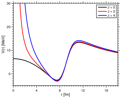
Figure 2: (Colour online) The two-body potentials for three different angular momenta (and corresponding potential depths). The potential depths are adjusted to give roughly the same energy as reflected by very similar minima. The depth of the interaction potential can be found in Table 1.

The variation of angular momentum allows us to investigate the influence of non-vanishing partial waves on the total three-body structure. It also allows comparison between ground and excited states of both the same and different angular momentum quantum numbers. Excited states from the present effective potential may be unavoidable when deeper-lying levels are occupied and Pauli-forbidden. The effect of changing the angular momentum can be seen in Fig. 2, where the potential depth in each case is adjusted to produce the same energy. The minima are then almost identical, and the only difference is the centrifugal barrier term deviating strongly at small distance.

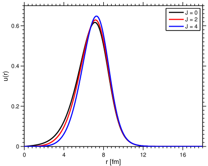
Figure 3: (Colour online) The two-body radial wave functions, $u$, for three different angular momenta (and corresponding potential depths).

The reduced radial ground state wave functions, $u(r)$, corresponding to the potentials in Fig. 2 are shown in Fig. 3. They are all spatially very similar and confined to a rather narrow region around the common minimum. This behaviour is unlike that of a core and a neutron which typically has a very wide spatial extent with a slowly decreasing tail jen04 . The narrow distribution is a direct consequence of the potentials in Fig. 2, where the $\alpha$-particle is confined by two very steep barriers on both sides of the minimum.

It is especially worth noting that the Coulomb interaction for $s$-waves is finite at $r=0$ as obtained by a homogeneous charge distribution within a sphere. The finite repulsion is still sufficient to push the wave function out to the surface almost precisely as for finite angular momenta with the additional diverging short-range repulsion. This angular momentum independent result is only achieved with a relatively large charge on the core-nucleus as for medium heavy or heavy nuclei.

Table 1: The two body energies and average sizes with a Ba-140 core and an $\alpha$-particle, where the angular momentum, $J$, and potential depth, $V_{0}$, have been varied. Positive energies, $E$, correspond to unbound states with negative binding. We denote ground, first excited, second excited, and third excited states by (G), (F), (S) and (T), respectively. Energies are in $\mathrm{MeV}$, and distances are in $\mathrm{fm}$.

$V_{0}$	$J$	State	$E$	$\langle r^{2}\rangle^{1/2}$
26.25	$0$	G.	0.1	7.0
		F.	4.3	5.9
		S.	7.4	5.4
27.1	$2$	G.	0.0	7.1
		F.	4.9	6.4
		S.	9.1	6.4
28.8	$4$	G.	0.1	7.2
		F.	5.7	6.8

The adjusted depths corresponding to $J=0,2,$ and $4$ are collected in Table 1. The resulting $\alpha$-core energies and the root-mean square radii are also given in this table for ground and all excited states. Due to the large barriers around the minimum these unbound states of positive energy are sufficiently well defined to allow computation of their radii. The potential depths are adjusted with angular momentum specifically to compensate the centrifugal barrier and leave the energy of the weakest bound state at essentially the same value. The intent is to have a slightly unbound two-body subsystem in the three-body system. The deepest potential will be used as the $\alpha$-core in the three-body system, as both the effect of changing angular momentum and the low lying excited states are of interest. Using the potential depth associated with $J=4$ in a calculation with $J=0$ may clearly produce more bound states. The radii of the states in Table 1 increase with increasing energy, but only moderately. The actual values would be strongly dependent on the radius of the potential. The peaks in Fig. 3 occur at around $7.2$ fm which is about the size of the core plus $\alpha$-particle charge radius. Thus fortunately, but not surprisingly, the $\alpha$-particle is located at the surface of the core.

III.2 Three-body formalism

The three-body calculations are carried out by use of the adiabatic hyper-spherical expansion method nie01 . First the Jacobi coordinates are defined as mass scaled vectors, ${\bf x}$ and ${\bf y}$, between one pair of particles, and between their center-of-mass and the third particle respectively. The relative orbital angular momenta, $l_{x}$ and $l_{y}$, are related to this choice of Jacobi coordinates. Three different choices are possible. The hyperspherical coordinates are defined by the hyperradius, $\rho$, and five hyperangles, $\Omega$. The (coordinate independent) definition of $\rho$ involves an arbitrary normalization mass, $m$, which has no influence on the result and is only used for notational convenience.

We first solve the hyper-angular part of the Faddeev equations for fixed average radius $\rho$. Each partial wave in each Faddeev component is expanded on the set of Jacobi polynomials from constants to the highest order defined by $K_{max}$. This provides a set of angular eigenvalues, $\lambda_{n}(\rho)$, and eigenfunctions, $\Phi_{n}(\rho,\Omega)$, where all quantities depend on $\rho$. The solution to these equations produce the effective potentials

$$V_{eff}(\rho)=\frac{\hbar^{2}}{2m}\left(\frac{\lambda_{n}(\rho)+15/4}{\rho^{2}}\right),$$ (8)

where $\lambda_{n}(\rho)$ is the crucial ingredient. The total wave function, $\Psi$, is expanded on the complete set, $\Phi_{n}$,

$$\Psi=\displaystyle\sum_{n}\rho^{-5/2}f_{n}(\rho)\Phi_{n}(\rho,\Omega),$$ (9)

where $f_{n}$ are the hyper-radial wave functions. They are determined by the coupled set of hyperradial equations arising from insertion of $\Psi$ into the Faddeev equations, that is

$$\left(-\frac{\partial^{2}}{\partial\rho^{2}}+\frac{1}{\rho^{2}}\left(\lambda_{n}(\rho)+\frac{15}{4}\right)-Q_{nn}-\frac{2mE}{\hbar^{2}}\right)f_{n}(\rho),$$

$$=\displaystyle\sum_{n^{\prime}\neq n}\left(2P_{nn^{\prime}}\frac{\partial}{\partial\rho}+Q_{nn^{\prime}}\right)f_{n^{\prime}}(\rho)\;,$$ (10)

where $E$ is the energy. The coupling terms, $P$ and $Q$, are given by

$$P_{nn^{\prime}}(\rho) =\left\langle\Phi_{n}\left|\frac{\partial}{\partial\rho}\right|\Phi_{n^{\prime}}\right\rangle_{\Omega},$$ (11)

$$Q_{nn^{\prime}}(\rho) =\left\langle\Phi_{n}\left|\frac{\partial^{2}}{\partial\rho^{2}}\right|\Phi_{n^{\prime}}\right\rangle_{\Omega}\;,$$ (12)

where the expectation values are over the hyperangles, $\Omega$, for fixed $\rho$. The convergence with the number of included adiabatic potentials is usually very fast, and only 4-6 are necessary in Eq. (10).

Figure 4: (Colour online) Effective potentials, Eq. (8), calculated from the five lowest $\lambda_{n}(\rho)$, for the case where $V_{0}=28.8\,$\mathrm{MeV}$$ and $J^{+}=0^{+}$. The horizontal lines correspond to the lowest, and first excited state of the lowest $\lambda_{n}(\rho)$, when it is approximated by a harmonic oscillator. It is noteworthy how similar the effective potentials are for the different $\lambda_{n}$ functions.

IV Core plus two-alpha properties

The previous section introduced the two-body potentials and the three-body formalism, which will be applied in the present section. Here ${}^{148}\text{Nd}$ is considered as a three body system consisting of a ${}^{140}\text{Ba}$ core and two $\alpha$ particles. These nuclei are chosen as they are at the edge of the $\alpha$ unstable region in Fig. 1. The purpose of this section is to study the nature of a general, relatively heavy, $\alpha$-Borromean system. As the same potential will be used for all partial waves, and as this potential was only adjusted to create a slightly unbound two-body system, energy levels cannot be expected to be reproduced. Of particular interest are the distributions among both the effective potentials and the partial waves, as well as the spatial distributions. In Sec. V.2 a detailed fine tuning of the individual partial waves is included for a similar system (${}^{142}\text{Ba}$ consider as ${}^{134}\text{Te}+\alpha+\alpha$) to reproduce both energy levels and electric transition probabilities.

The calculations presented here treat the core as an inert particle with angular momentum and parity $0^{+}$. Therefore, the effects arising from excitations of the ¹⁴⁰Ba core, in the ¹⁴⁸Nd case, or the ¹³⁴Te core, in the ¹⁴²Ba case, into the 2⁺ excited state (at 0.60 MeV in ¹⁴⁰Ba and 1.28 MeV in ¹³⁴Te) will not be considered.

The solutions are obtained in two steps. First the angular wave functions are calculated and second we solve the coupled radial set of equations. In the first step both angular wave functions, and radial potentials, and their couplings are produced. In the first subsection, we discuss the properties of these solutions, and in the second subsection we present the radial structure in simple geometric terms.

IV.1 Angular three-body structure

The five lowest of the effective potentials given in Eq. (8) are shown in Fig. 4 for angular momentum and parity, $0^{+}$, and a given appropriate strength, $V_{0}=28.8$ MeV, of the Woods-Saxon potential. The lowest minimum value is about $-8$ MeV and located close to $\rho\approx 20$ fm. The potential has a rather steep barrier rising to about $+11$ MeV at roughly $27$ fm, after which it decreases slowly towards zero as $\rho$ increases to infinity. The fall-off is proportional to $1/\rho$ because the Coulomb potentials are responsible for this long-range behaviour. This implies proportional fall-off for all potentials, since the large-distance Coulomb interactions are the same for all adiabatic potentials. The increase of the potential for small $\rho$ is due to the centrifugal barrier behaviour of $1/\rho^{2}$, while the Coulomb potentials remain finite through the assumption of homogeneous charge distributions.

The higher-lying adiabatic potentials are remarkably similar to the lowest and each only shifted by about $1.5$ MeV, very crudely independent of $\rho$. The zero point motion of the best fit of the lowest potential by a one-dimensional oscillator is about $2.7$ MeV ($\hbar\omega\approx 5.5$ MeV). The first excited oscillator energy is then at about $8.5$ MeV above the oscillator bottom. The shifted zero point in our potential is at about $-8$ MeV producing two oscillator estimates at about $-5.0$ MeV and $+0.5$ MeV as indicated by the horizontal lines in Fig. 4.

The distance between neighbouring adiabatic potentials is roughly about $1.5$ MeV. The first excited state in the lowest potential at about $+0.5$ MeV is then at about the same position as the ground state of the fourth potential, which is estimated to be at about $4\times 1.5$ MeV $+2.7$ MeV above the lowest minimum at $-8$ MeV, that is $+0.7$ MeV. This implies that the wave functions of the lowest-lying two states in the $0^{+}$ spectrum can be expected almost entirely built on individual potentials, unless of course the couplings between the adiabatic potentials are unusually strong. The third excited state could energy-wise instead be composed of comparable components from first and fourth potentials.

Higher angular momentum potentials are rather similar but with minima shifted upwards by the centrifugal barrier amounting to roughly $0.4$ MeV and $1.4$ MeV for $2^{+}$ and $4^{+}$, respectively. The large distance behaviour is essentially maintained, whereas the increase and eventual divergence at short distance accelerate with angular momentum as in Fig. 2. Finally, modest variation of the two-body potential strength will only displace the curves slightly, and the effect is most noticeable at large distances, where it has no effect on the bound state structure.

Table 2: The three body energies of ${}^{148}\text{Nd}$ $(^{140}\text{Ba}+\alpha+\alpha)$, as well as average $\alpha$-$\alpha$ and $\alpha$-core distances for different angular momenta with $V_{0}=28.8$ MeV, $a=0.65$ fm, $R=9.1$ fm, $R_{C}=7.4$ fm. The weights of the contributing adiabatic potentials are given for each state in the last five columns. All energies are in $\mathrm{MeV}$ and all distances are in $\mathrm{fm}$.

				Weights of potentials $(\%)$
$J^{\pi}$	$E$	$\langle r_{\alpha\alpha}^{2}\rangle^{\frac{1}{2}}$	$\langle r_{\alpha c}^{2}\rangle^{\frac{1}{2}}$	1	2	3	4	5
$0^{+}$	-4.9	4.8	6.9	95	4	0	1	0
$0^{+}$	-3.7	12.0	7.0	7	92	1	0	0
$0^{+}$	-2.6	10.9	7.0	3	1	94	2	0
$0^{+}$	-0.8	10.2	7.2	17	3	2	74	4
$2^{+}$	-4.5	4.7	7.0	95	5	0	0	0
$2^{+}$	-3.3	12.0	7.0	7	89	3	1	0
$2^{+}$	-2.3	9.6	7.0	2	4	22	70	2
$2^{+}$	-0.1	10.9	7.4	2	1	9	22	66
$4^{+}$	-3.5	4.9	7.0	95	4	0	0	0
$4^{+}$	-2.4	12.4	7.1	7	84	9	0	0
$4^{+}$	-1.6	9.7	7.0	1	10	81	6	2
$4^{+}$	-0.7	8.8	7.0	0	1	10	78	10

The calculated energies are given in Table 2 for the potential strength $V_{0}=28.8$ MeV and different angular momenta. Decreasing the attraction to $V_{0}=26.25$ MeV only one $0^{+}$ state ($2^{+}$, $4^{+}$) is bound at $-0.2$ MeV. A further increase of strength to $V_{0}=27.1$ MeV provides two bound $0^{+}$ states at $-1.8$ MeV and $-0.6$ MeV, and two bound $2^{+}$ states at $-1.3$ MeV and $-0.2$ MeV. When $V_{0}=28.8$ MeV, corresponding to Fig. 4, we find four bound state solutions for each set of quantum numbers, $0^{+}$, $2^{+}$ and $4^{+}$. Thus, the three-body bound states appear much faster and more abundantly than the two-body $\alpha$-core potentials in Fig. 2. The oscillator estimate of about $-5.0$ MeV and $0.5$ MeV for the two lowest $0^{+}$ states built on the lowest adiabatic potential is rather accurate as only one corresponding bound state appears at $-4.9$ MeV, see Table 2. Unbound resonance states are not computed until Sec. V.2, where ${}^{142}\text{Ba}$ is examined in detail.

The structure of these states is known through the calculated properties of the wave functions. We consider first the contributions from the different adiabatic potentials to the individual states. Only five potentials are necessary to ensure accurate radial solutions. The relative weights in Table 2 are remarkably simple with one entirely dominating potential for all wave functions. The two weakest bound $2^{+}$ states are the most fractionated with a division of ($22\%$, $70\%$) and ($22\%$,$66\%$) on third and fourth, and fourth and fifth potentials, respectively.

In general, each potential then essentially carries the full weight of a given state, such that the lowest potential corresponds to the lowest energy, the second potential and the second lowest energy are related, etc. This confirms the main conclusion of one adiabatic potential per state obtained from the estimate by use of an oscillator approximation without couplings between potentials. The third excited $0^{+}$ state begins to have contributions from both first and fourth adiabatic potentials. The excitation on the lowest potential competes with the lowest energy on the fourth potential, and two configurations arise. The second excited $2^{+}$ state is fractionated between third and fourth potentials, now because the potentials happen to be rather close-lying and the couplings are therefore more effective.

Table 3: The weights of each partial wave for the potential specified in Table 2. Here $l_{x}$ denotes the relative angular momentum between the two particles, and $l_{y}$ denotes the angular momentum of the third particle relative to the center of mass of the first two particles. The fifth column give the order, $K_{max}$, of the Jacobi polynomium used for the corresponding partial wave. The last four columns each describe ground (G), first (F), second (S) and third (T) excited states. Components where all states have a weight less than $0.04$ are omitted.

$J^{\pi}$	Jacobi	$l_{x}$	$l_{y}$	$K_{max}$	G.	F.	S.	T.
$0^{+}$	$\alpha$-$\alpha$	0	0	80	0.79	0.73	0.72	0.72
		2	2	60	0.19	0.22	0.22	0.22
		4	4	50	0.02	0.04	0.05	0.05
$0^{+}$	$\alpha$-c	0	0	100	0.43	0.51	0.04	0.07
		1	1	80	0.39	0.48	0.09	0.06
		2	2	60	0.10	0.01	0.85	0.01
		3	3	50	0.00	0.00	0.00	0.79
$2^{+}$	$\alpha$-$\alpha$	0	2	70	0.82	0.07	0.26	0.04
		2	0	70	0.05	0.72	0.45	0.54
		2	2	50	0.05	0.08	0.16	0.29
		2	4	40	0.07	0.02	0.06	0.01
		4	2	40	0.01	0.09	0.05	0.05
		4	4	30	0.00	0.01	0.01	0.05
$2^{+}$	$\alpha$-c	0	2	70	0.18	0.25	0.02	0.00
		2	0	70	0.19	0.23	0.03	0.00
		1	1	50	0.39	0.50	0.03	0.00
		2	2	50	0.06	0.01	0.05	0.23
		1	3	40	0.04	0.00	0.38	0.07
		3	1	40	0.05	0.00	0.37	0.07
		3	3	40	0.01	0.00	0.03	0.35
		2	4	40	0.00	0.00	0.01	0.05
		4	2	40	0.00	0.00	0.02	0.04
		4	4	30	0.00	0.00	0.03	0.05
$4^{+}$	$\alpha$-$\alpha$	2	2	80	0.09	0.15	0.34	0.27
		0	4	50	0.78	0.02	0.07	0.08
		4	0	50	0.00	0.68	0.15	0.26
		4	2	48	0.01	0.03	0.18	0.02
		2	4	48	0.06	0.03	0.18	0.27
		6	2	20	0.00	0.06	0.02	0.02
$4^{+}$	$\alpha$-c	2	2	80	0.40	0.51	0.03	0.02
		1	3	80	0.20	0.26	0.02	0.00
		3	1	66	0.22	0.22	0.03	0.00
		2	4	68	0.01	0.00	0.00	0.20
		4	2	68	0.01	0.00	0.00	0.21
		4	0	50	0.04	0.00	0.41	0.03
		0	4	50	0.03	0.00	0.42	0.03
		4	4	50	0.00	0.00	0.01	0.06
		5	1	40	0.00	0.00	0.01	0.09
		1	5	40	0.00	0.00	0.01	0.10

The structure revealed by the partial wave decomposition of the wave functions is seen in Table 3, where only the contributions amounting to more than $4\%$ are included. We give decompositions in both the two different Jacobi coordinate sets. Here it is worth noticing that only even angular momenta are allowed between the two $\alpha$-particles due to the identical boson characteristics. We first emphasize that the small attractions, where the energies approach all the way down to zero, all down to the percent level produce the same partial wave decomposition independent of the specific energy. We therefore only show the results for one strength. The structures remain unchanged because essentially only the potential energies are moved corresponding to a shifted energy scale.

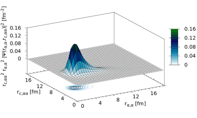
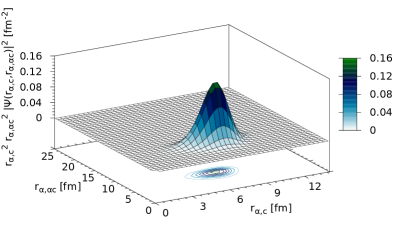
Figure 5: (Colour online) The probability distribution for the $0^{+}$ ground state wave with the $\alpha$-core potential specified in Table 2. Projected contour curves are shown at the bottom of each figure. The distance variables correspond to the two different Jacobi sets, where top and bottom panels are for the first and second Jacobi sets, respectively.

For the $0^{+}$ states we find more than $70\%$ of $\alpha$-$\alpha$ $s$-waves in all solutions, while the $d$-waves absorb most of the remaining probabilities. This is obviously consistent with the stronger $\alpha$-$\alpha$ attraction in the lowest partial waves. However, the $\alpha$-core potential may prefer another competing structure. The two lowest $0^{+}$ states have roughly equal amounts of $\alpha$-core relative $s$- and $p$-waves, whereas the third and fourth $0^{+}$ states are dominated by $d$- and $f$-waves, respectively. In combination with the results from Table 2 this indicates that these higher-lying adiabatic potentials are dominated by $d$- and $f$-waves.

The $2^{+}$ states must have non-zero angular momentum partial waves. The most favourable structure seen in Table 3, is apparently $s$-waves between the two $\alpha$-particles but a distribution for the $\alpha$-core structure of equal $s$- and $d$-waves and twice as much $p$-waves. In contrast, the first excited state has dominating $\alpha$-$\alpha$ $d$-waves and comparable to the ground state contributions from $g$-waves. The second and third excited states have also $\alpha$-$\alpha$ $d$-waves as the largest components. The $\alpha$-core contributions are now moved to roughly equal $p$- and $f$-waves, and comparable $d$- and $f$-waves, respectively for second and third excited state.

The $4^{+}$ states must have even larger finite angular momentum contributions than the $2^{+}$ states. In Table 3 we find again that $s$-waves dominate for ground state, while the first excited state is dominated by $g$-waves in the $\alpha$-$\alpha$ subsystem. In the $\alpha$-core subsystem, these two states have the largest contributions from $d$-waves and roughly half as much for $p$- and $f$-waves. The third and fourth $4^{+}$ states have in the $\alpha$-$\alpha$ subsystem more than $50\%$ of $d$-waves and roughly half as much $g$-waves. In the $\alpha$-core subsystem $s$- and $g$-, and $d$- and $g$-wave components are about equal, respectively for the third and fouth $4^{+}$ states. The higher-lying states receive significant contributions from more partial waves than ground and excited states.

These rather complicated variations in structure for the different states are dictated by minimizing the total energies. This involves combinations of the two-body interactions which in the present cases always prefer the lowest partial waves. The final results are then obtained by combining the minimization with total angular momentum conservation, partial wave couplings, and orthogonality of all pairs of states.

IV.2 Radial structure

The angular eigenvalues, $\lambda_{n}$, provide information about the crucial radial potentials, which in turn through Eq. (10) determine the radial wave functions, $f_{n}(\rho)$. The linear combination with the angular parts, $\Phi_{n}$, from Eq. (9) gives access to complete information about each of the solutions. We shall in particular be concerned with probability distributions for the $\alpha$-$\alpha$ and $\alpha$-core distances.

In Fig. 5 we show the probability distribution for the $0^{+}$ ground state in two coordinate systems corresponding to the two different Jacobi coordinates. The structure is relatively simple with only one peak at an $\alpha$-$\alpha$ distance of about $4$ fm from the top panel and an $\alpha$-core distance of about $7$ fm from the bottom panel of Fig. 5.

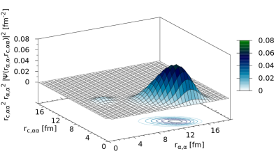
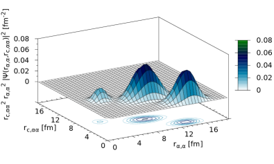
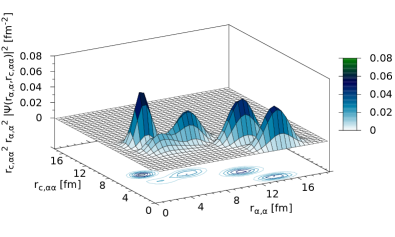
Figure 6: (Colour online) The same as top panel of Fig. 5. for the three excited $0^{+}$ states.

The probability distributions for the excited $0^{+}$ states are shown in Fig. 6 for the first Jacobi set where the $x$-coordinate is between the two $\alpha$-particles. In all these excited states we find probability distributions between core and $\alpha$-particle almost identical to that of the ground state as shown in the lower part of Fig. 5. Consequently, we do not show these distributions. However, the identical distributions demonstrate that the $\alpha$-particles strongly prefer to be located at the surface of the core as for the isolated two-body system with the wave function shown in Fig. 3. The reason is that the $\alpha$-core potential overrules all other possible effects when determining the three-body structure. Apparently the $\alpha$-$\alpha$ potential is strongly attractive and the potential energy minimum is rather narrow and deep.

However, the $\alpha$-$\alpha$ distribution varies from top to bottom in Fig. 6, and they are also different from the ground state distribution. The first excited state shows a broader distribution around the $\alpha$-$\alpha$ distance of $13$ fm with a marginal reminiscence of a peak at the ground state location of about $4$ fm. The second excited state has three peaks at $\alpha$-$\alpha$ distances of about $14$ fm, $9$ fm and $4$ fm. The third excited $0^{+}$ state continues the trend by containing four peaks at $\alpha$-$\alpha$ distances of $14$ fm, $12$ fm, $7$ fm, and $4$ fm. These different structures reflect the different structures of the corresponding adiabatic potentials, which deliver the dominating contributions to each of the excited states.

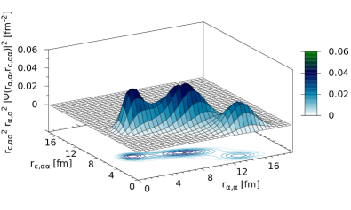
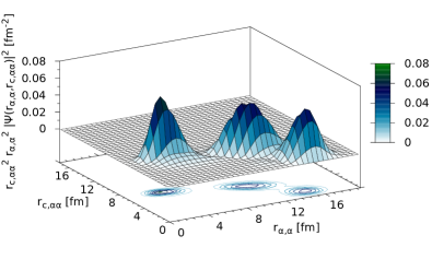
Figure 7: (Colour online) The same as top panel of Fig. 5. for the second and third excited $2^{+}$ states.

The probability distributions for the lowest two $2^{+}$ states are very similar to the $0^{+}$ distributions in Fig. 5. Also the $\alpha$-core distributions are remarkably similar for the computed higher-lying $2^{+}$ states. The $\alpha$-$\alpha$ distribution for the second excited $2^{+}$ state in Fig. 7 reveals a much broader distribution. It is almost without peaks but with a ridge stretching from $\alpha$-core distances between $10$ fm and $4$ fm with a corresponding increase of the distance of the core from the $\alpha$-$\alpha$ center of mass. The third excited $2^{+}$ state is also shown in Fig. 7 exhibiting distinct peaks at distances of about $15$ fm, $11$ fm and $4$ fm.

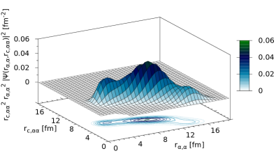
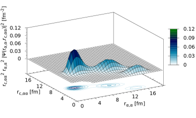
Figure 8: (Colour online) The same as top panel of Fig. 5. for the second and third excited $4^{+}$ states.

The $\alpha$-core distributions for the $4^{+}$ states are again almost indistinguishable from the previously computed distributions for the other angular momenta, such as the example shown in the lower panel of Fig. 5. The $\alpha$-$\alpha$ distribution for the first excited $4^{+}$ state resembles the same distribution for both first excited $0^{+}$ and $2^{+}$ states. The distribution for the second excited $4^{+}$ state is shown in Fig. 8, where the peak structure again is smeared out and the largest probability peak is at around $11$ fm. For the third excited $4^{+}$ state in Fig. 8, the $\alpha$-$\alpha$ distribution displays three peaks at around $14$ fm, $10$ fm and $4$ fm.

In summary, the many different probability distributions all have the remarkable property of one peak in the $\alpha$-core distance. The corresponding interaction is strong and essentially a surface attraction due to centrifugal and Coulomb potentials. In contrast the $\alpha$-$\alpha$ distributions exhibit very large variations from one peak to several peaks or rather smeared out distributions. However, all these distributions have fortunately a sharp cut-off at small distances where the $\alpha$-particles would beginning to overlap.

The tempting interpretation in terms of simple geometric structures is then only meaningful when one not too broad peak contains a large fraction of the probability. It may still be rewarding to look at average distance properties as the root mean square radii given in Table 2. Once more we emphasize that the $\alpha$-core root mean square radius is remarkably constant for all states. We can then conclude that the $\alpha$-particles are located on spheres corresponding to this radius around the core.

The average $\alpha$-$\alpha$ distances for the ground states of any angular momentum are $4.8$ fm which is similar to, although about $1$ fm less than, the same quantity, $5.95$ fm for the two-$\alpha$ structure of ⁸Be. Combined with the $70\%$ of $s$-waves in all these ground states we conclude that these three-body states resemble a core plus ⁸Be in its ground state. The first excited states of all three angular momenta are also very similar to each other but now with more than $70\%$ of $\alpha$-$\alpha$ $2^{+}$ structure and with a much larger distance of about $12$ fm. This structure is far from any excited state of ⁸Be, and these structures in fact resemble a linear structure with the core in the middle.

The second and third excited states exhibit much more complicated structures which cannot be collected into one simple configuration. However, they can be described as containing three or maybe even four components each with different configurations. The resulting probability distributions are more smeared out but both ⁸Be like ground state structures, linear $\alpha$-core-$\alpha$ chain-configurations, and intermediate structures are present in each state.

V Observable consequences

The general structures for systems with weak binding of one- and two $\alpha$-particles are discussed in the previous section. We shall here first compare to measured properties of ${}^{148}\text{Nd}$, which was considered in Sec. IV as a general representative of $\alpha$-Borromean structures in relatively heavy nuclei. In the second subsection we shall discuss the results obtained from fine-tuning the interaction parameters to be appropriate for the only known (apart from ¹²C) even-even Borromean two-$\alpha$ nucleus, ¹⁴²Ba.

V.1 Properties of ¹⁴⁸Nd $(^{140}\text{Ba}+\alpha+\alpha)$

The spectra in Table 2 for the lowest energies of the $0^{+}$, $2^{+}$, and $4^{+}$ states present a rotational sequence, $(0.0,0.4,1.4)$, with rigid body moment of inertia, ${\cal I}$ corresponding to $\hbar^{2}/{\cal I}\approx 0.14$ MeV. This implies a distance, $r_{c,\alpha\alpha}$, of about $6.19$ fm between the core and the center of mass of two $\alpha$-particles, which is almost identical to the value derived from Table 2. Furthermore, this is in complete agreement with indistinguishable geometric properties for these three $0^{+}$, $2^{+}$ and $4^{+}$ states shown in Fig. 5 for the $0^{+}$.

The conclusion is that these states form a rotational band. The schematic rules for rotational B(E2)-transition probabilities are then obeyed for a core plus a two-$\alpha$ structure rotating around their common center of mass. The absolute values of the electromagnetic transition probabilities are proportional to the intrinsic electric quadrupole moment, $Q_{0}$, of the same structure. For a relatively heavy core we have $Q_{0}\approx 8er_{c,\alpha\alpha}^{2}\approx 307$ e fm², where $4$ e is the charge of the combined two $\alpha$-particles. The single-particle value, $Q_{sp}\approx 75$ e fm², is about four (the charge) times smaller, provided the same radius is used in both estimates.

Let us now compare these numerical average results to measured values for ¹⁴⁸Nd nic14 . First, the observed excitation energies do not follow the simple rotational model predictions. The energies of the $4^{+}$ state is $2.5$ times larger than the energies of the $2^{+}$ states. If anything this is closer to the vibrational model value of $2$ rather than $3.3$ valid for rotations. The vibrational picture does not match any better by combining the second $0^{+}$ and $2^{+}$ states.

Transition probabilities contain more detailed information about structures, but only rather uncertain data are available for these nuclei. For ¹⁴⁸Nd the available measurements of B(E2) values are, $B(E2;0\rightarrow 2)=1.37$ e² b², $B(E2;2\rightarrow 4)=0.784$ e² b², and the quadrupole moment, $Q^{(2)}=-1.46$ e b, for the $2^{+}$ state. Transforming these transition values into the down going probabilities we get the ratio $0.78\times 25/(1.37\times 9)=1.58$ which is comparable to $1.41$ from the rotational model but also not too far from the vibrational value of $2$. The quadrupole moment is related to the intrinsic quadrupole moment by $Q_{0}=-Q^{(2)}7/2=511$ e fm² where our model value of $307$ e fm² is $1.7$ times smaller than measured.

Considering the same effective potentials were used for all partial waves, an agreement within a factor of two is better than what could have been expected. This is in spite of the fact that the model forms a rotational spectrum, while the data do not contain simple, strictly rotational or vibrational features. It is also worth noting that the simple model produced an energy spectrum where the energy of the $4^{+}$ state is $2.5$ times larger than the energy of the $2^{+}$ state, same as for ${}^{148}\text{Nd}$. This suggests that ${}^{148}\text{Nd}$, and nuclei similar to it, might well be described as two-$\alpha$ structures in their low-lying states.

The model with the same average parameters in the radial effective potential is independent of angular momentum and known to be very inaccurate for odd parity states. This average model can only marginally distinguish between odd and even parity states, since the centrifugal barrier varies continuously with orbital angular momentum. Only the Bose character of the $\alpha$-particles is able to give small differences due to parity. On the other hand, low-energy nuclear spectra with only very few exceptions are dominated by the positive parity states while negative parity states are located at higher excitation energies. In nuclear few-body models this feature is accounted for by partial wave (angular momentum and parity) dependent effective potentials. A proper comparison to data therefore involves detailed input and careful search for suitable nuclei where the few-body structure is possible.

V.2 Properties of ¹⁴²Ba $(^{134}\text{Te}+\alpha+\alpha)$

The most tempting nuclei to investigate are Borromean two-$\alpha$ systems. Searching the available masses for candidates we find only one known even-even nucleus, ¹⁴²Ba ($\alpha+\alpha+^{134}$Te), of that structure. The exception of ¹²C ($\alpha+\alpha+\alpha$) is special since the core also consists of an $\alpha$-particle. Nuclear few-body models must assume decoupling of intrinsic and relative cluster degrees of freedom. Therefore the intrinsic degrees of freedom preferably should be difficult to excite either by weak couplings or by unreachable high excitation energy.

Table 4: The Woods-Saxon depths, $V_{0}$, reproducing the resonance energies, $E_{res}$, for the different angular momentum and parities, $J^{\pi}$, in ¹³⁸Xe $(^{134}\text{Te}+\alpha)$ son03 . There is no known $5^{-}$ state in the ${}^{138}\text{Xe}$ excitation spectrum, so the same potential depth as for $3^{-}$ was used. The energy of the $0^{+}$ state is determined by the $\alpha$ separation energy through Eq. (13). All energies are in $\mathrm{MeV}$.

$J^{\pi}$	$0^{+}$	$2^{+}$	$4^{+}$	$6^{+}$	$1^{-}$	$3^{-}$	$5^{-}$	Other
$E_{res}$	0.138	0.727	1.211	1.419	2.004	2.153	-
$V_{0}$	24.423	24.568	25.787	28.2	22.641	23.746	23.746	24.568

The present case has ¹³⁴Te as the core where the lowest excited state is a $2^{+}$ state at 1.279 MeV son04 . By adjusting the partial wave interactions the polarization is fully included in the adopted effective potential on the two-body level. If present, an $\alpha$-cluster structure should be seen as resonances in $\alpha$-core scattering, that is as ¹³⁸Xe states son03 . The energy of the $0^{+}$ ground state is then determined by the $\alpha$ separation energy

$$E_{res}(0^{+})=-\left(B(^{138}\text{Xe})-B(^{134}\text{Te})-B_{\alpha}\right).$$ (13)

This provides the depth of the radial potentials for each angular momentum and natural parity. We choose the same radial Woods-Saxon shape with the same radius and diffuseness parameters as used above. We only adjust the depth to reproduce the measured resonance energies in ¹³⁸Xe ($\alpha+^{134}$Te). The resulting values are given in Table 4.

Table 5: The same as Table 2 for ¹⁴²Ba $(^{134}\text{Te}+\alpha+\alpha)$ using the potential depths specified in Table 4 for the individual partial waves. The column labelled $E_{exp}$ is the measured value from joh11 , where the energy of the $0^{+}$ state is determined by the two $\alpha$ separation energy. Two first excited states, indicated by $(F)$, are also included. The last five columns specifies the individual weights of the five lowest potentials.

						Weights $(\%)$
$J^{\pi}$	$E_{exp}$	$E_{cal}$	$E_{cal}-E_{exp}$	$\langle r_{\alpha\alpha}^{2}\rangle^{\frac{1}{2}}$	$\langle r_{\alpha c}^{2}\rangle^{\frac{1}{2}}$	1	2	3	4	5
$0^{+}$	-0.16	0.11	0.27	7.8	7.0	99	1	0	0	0
$2^{+}$	0.20	0.50	0.30	7.5	7.1	99	0	0	1	0
$4^{+}$	0.68	0.98	0.30	7.4	7.1	96	2	1	0	0
$1^{-}$	1.17	1.11	-0.06	4.2	7.1	98	1	0	0	0
$3^{-}$	1.13	1.37	0.24	4.3	7.1	96	2	1	0	1
$2^{+}(F)$	1.26	1.05	-0.21	5.9	7.1	0	98	1	1	0
$6^{+}$	1.31	0.90	-0.41	6.6	7.2	95	3	2	0	0
$0^{+}(F)$	1.38	1.59	0.22	9.3	7.1	2	96	1	0	0

The energies and sizes of the three-body eigenstates are given in Table 5, together with the distribution of weights on the different adiabatic potentials, and the experimentally measured energies joh11 . Here the ground state energy is determined by the two $\alpha$ separation energy. Also included in Table 5 is the difference between the calculated and the measured energies.

The absolute values of the calculated energies are seen to be displaced by roughly $0.3\,$\mathrm{MeV}$$ for four of the five lowest states. A slight displacement is not surprising as no attempt has been made to account for explicit three body effects. A distinct three-body potential could be added, but it would be an ad hoc addition adjusted to fit the desired spectrum. More interesting are the relative distances between individual levels in the calculated spectrum, and they agree very well with relative distances between the experimental measurements. The calculated relative distances between the $0^{+}$, and the $2^{+}$, $4^{+}$, and $3^{-}$ states only differ by about $0.03\,$\mathrm{MeV}$$ from the relative distances in the experimental spectrum. The only exception among the lowest states is the $1^{-}$ state, which does not agree with the shifted spectrum. Its absolute value actually agrees more closely with the experimental value. This agreement is most likely coincidental, and merely the result of counteracting offsets. It may be of interest that in the symmetry classification of the corresponding states in the related system ${}^{12}\text{C}$ mar14 the lowest $1^{-}$ state appears in a different ”band” than the $0^{+}$, $2^{+}$, $3^{-}$, and $4^{+}$ states.

For the three remaining, higher lying states, the deviations become more erratic. The difference between the calculated and the experimental values is no longer close to constant. This might indicate a limit to the model given by the core excitation energy.

The weights of the individual potentials are as expected from the results of the previous sections. Each state is dominated by a single adiabatic potential. The lowest potential dominates for all non-excited states, while the second potential dominates for the first excited states. The coupling between different potentials must then be very weak, even when the potentials of each partial wave are adjusted individually.

The average $\alpha$-core distance is again constant at around $7.1\,$\mathrm{fm}$$, which implies that the $\alpha$ particles are still placed at the surface of a sphere around the core. The probability distributions between the core and the $\alpha$-particle are also identical to the distribution seen in the lower part of Fig. 5, and is therefore not included. The average $\alpha$-$\alpha$ distances, on the other hand, are very different from the ground state values in Table 2, at least for the even parity states. However, the average values are somewhat misleading. In Fig. 9 the probability distributions for the $0^{+}$, $2^{+}$, $4^{+}$, and $6^{+}$ states are shown. The same peak as in Fig. 5 at an $\alpha$-$\alpha$ distance of roughly $4\,$\mathrm{fm}$$ is seen for all three states. The large average values are caused by the appearance of a much smaller peak at an $\alpha$-$\alpha$ distance of about $13\,$\mathrm{fm}$$. This almost constitutes a line structure, with $\alpha$ particles on opposite sides of the core.

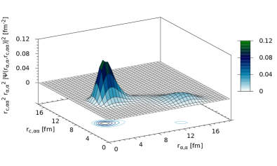
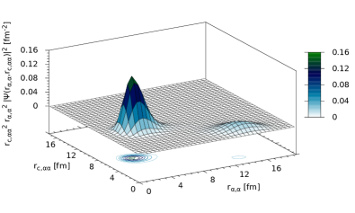
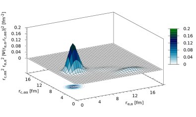
Figure 9: (Colour online) The same as top panel of Fig. 5. for the lowest $0^{+}$, $2^{+}$, $4^{+}$, and $6^{+}$ ¹⁴²Ba states.

The probability distribution for first excited $0^{+}$ and $2^{+}$ states are seen in Fig. 10. The distribution of the first excited $0^{+}$ is similar to the top panel of Fig. 6, only with the large peak at the slightly smaller $\alpha$-$\alpha$ distance of $10\,$\mathrm{fm}$$. The distribution of the first excited $2^{+}$ state is unusual compared with the first excited states examined previously. It is almost identical to the distribution of the $2^{+}$ ground state seen in the second panel of Fig. 9.

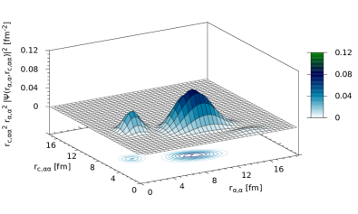
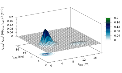
Figure 10: (Colour online) The same as top panel of Fig. 5. for the first excited $0^{+}$ (above), and $2^{+}$ (below) states of ¹⁴²Ba.

On the other hand, the average distances for the odd parity states agree reasonably well with the earlier results. The probability distribution for the $1^{-}$, and $3^{-}$ states are seen in Fig. 11. They are identical to the upper part of Fig. 5. The single peak is then well described by the average distance in Table 5.

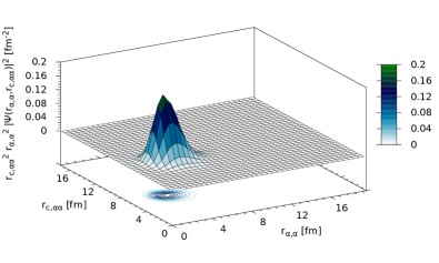
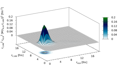
Figure 11: (Colour online) The same as top panel of Fig. 5. for the lowest $1^{-}$, and $3^{-}$ states of ¹⁴²Ba.

The contributions from the different partial waves are listed in Table 6. The overall tendencies are the same as in Table 3, but the specific weights have changed slightly. The relative angular momentum between the two $\alpha$ particles is dominated by $s$-waves for all but the $6^{+}$ state, although to a lesser extent than before. Particularly interesting are the odd parity states which were not included earlier. The $1^{-}$ state is the only state which have a dominating contribution from $p$-waves to the relative $\alpha$-core angular momentum. This could be part of the explanation as to why the $1^{-}$ state deviates from the other low lying states. Likewise, the $3^{-}$ is the only state to have a significant $f$-wave contribution to the $\alpha$-core angular momentum. For the $3^{-}$ state there is a roughly even contribution from $s$-, $p$-, $d$-, and $f$-waves. The higher lying $6^{+}$ and $5^{-}$ states have a much more scattered distribution of partial waves, in particular for the $\alpha$-core system. However, these results are less reliable, as the states are outside the energy region, which can the model can reasonably be expected to cover.

Table 6: The same as Table 3 with ¹⁴²Ba for the states from Table 5

$J^{\pi}$	Jacobi	$l_{x}$	$l_{y}$	$K_{max}$	G	F
$0^{+}$	$\alpha$-$\alpha$	0	0	80	0.80	0.62
		2	2	60	0.18	0.30
		4	4	50	0.02	0.07
$0^{+}$	$\alpha$-c	0	0	100	0.70	0.27
		1	1	80	0.04	0.02
		2	2	60	0.17	0.67
$2^{+}$	$\alpha$-$\alpha$	0	2	70	0.62	0.06
		2	0	70	0.20	0.44
		2	2	50	0.11	0.46
		2	4	40	0.04	0.02
$2^{+}$	$\alpha$-c	0	2	70	0.35	0.00
		2	0	70	0.35	0.00
		2	2	50	0.09	0.17
		3	3	40	0.00	0.04
		2	4	40	0.02	0.05
		4	2	40	0.02	0.05
		4	4	30	0.01	0.30
		6	6	30	0.01	0.06
$4^{+}$	$\alpha$-$\alpha$	2	2	80	0.04
		0	4	50	0.63
		4	0	50	0.18
		2	4	48	0.08
$4^{+}$	$\alpha$-c	2	2	80	0.44
		4	0	50	0.17
		0	4	50	0.16
$1^{-}$	$\alpha$-$\alpha$	0	1	75	0.81
		2	1	65	0.09
		2	3	55	0.09
$1^{-}$	$\alpha$-c	0	1	75	0.22
		1	0	75	0.23
		2	1	55	0.15
		1	2	55	0.15
		2	3	55	0.05
		3	2	55	0.05
$3^{-}$	$\alpha$-$\alpha$	0	3	75	0.69
		2	3	55	0.26
$3^{-}$	$\alpha$-c	0	3	75	0.14
		3	0	75	0.15
		2	1	65	0.12
		1	2	65	0.12
		4	1	41	0.07
		1	4	41	0.06
$6^{+}$	$\alpha$-$\alpha$	0	6	100	0.23
		6	0	90	0.06
		2	4	90	0.06
		2	6	90	0.52
		6	2	80	0.08
$6^{+}$	$\alpha$-c	0	6	100	0.14
		6	0	90	0.14
		2	4	90	0.08
		4	2	80	0.07
		4	6	40	0.04
		6	4	40	0.04
		6	6	50	0.14

The calculated dipole and quadrupole transition probabilities are presented in Table 7. Included are both the results for the two-body ${}^{138}\text{Xe}$ $(^{134}\text{Te}+\alpha)$ and the three-body ${}^{142}\text{Ba}$ $(^{134}\text{Te}+2\alpha)$ systems. The transition probabilities are given by

$$B(E\lambda;J\rightarrow J^{\prime})=Q_{0}^{2}\langle J0\lambda 0|J^{\prime}0\rangle^{2},$$ (14)

where $\langle J0\lambda 0|J^{\prime}0\rangle$ is the Clebsch-Gordan coefficient coupling the states $J$ and $J^{\prime}$. In the two-body system $Q_{0}$ for the quadrupole transition is

$$Q_{0}=\sqrt{\frac{5}{16\pi}}2r_{\alpha c}^{2}\frac{z_{\alpha}em_{c}^{2}+z_{c}em_{\alpha}^{2}}{(m_{\alpha}+m_{c})^{2}},$$ (15)

while for the dipole transition $Q_{0}$ is

$$Q_{0}=\sqrt{\frac{3}{4\pi}}r_{\alpha c}\frac{z_{\alpha}em_{c}-z_{c}em_{\alpha}}{(m_{\alpha}+m_{c})}.$$ (16)

Here $m_{\alpha}$ and $m_{c}$ are the masses, $z_{\alpha}$ and $z_{c}$ are the proton numbers, and $e$ is the elementary charge. The $\alpha$-core distance used is $7.1\,$\mathrm{fm}$$, as given in Table 5. There are two $\alpha$ particles in the three-body system, so twice the $\alpha$ mass, and twice the $\alpha$ charge is used. Also the distance is replaced by the distance between the core and the $\alpha$-$\alpha$ system, $r_{c,\alpha\alpha}$. The value used is not the average value from Table 5, but the peak value of $6.8\,$\mathrm{fm}$$ from Figs. 9 and 11.

Unfortunately, only a few experimental values are available at the moment, as seen in Table 7. Both the dipole and the quadrupole transition probabilities are relatively small, but for different reasons. The intrinsic particle degrees of freedom do not contribute to the rotational motion, because of the mass difference, so small values of the quadrupole transition probabilities are inherent in cluster rotations. Considering first the quadrupole transitions in ${}^{142}\text{Ba}$, the model values are seen to be around $1.8$ times too large. It should be noted that the distance enters in the fourth power, so changing it slightly will have significant impact on the result. As this distance is dictated by Coulomb and centrifugal barriers, it does to some degree depend on the chosen parameters. This makes the agreement surprisingly good. The ratio between the states is $0.24/0.34=0.71$ in the model, which is very much comparable to the ratio of $0.77$ for the experimental values. Very few other calculations are available, but specialized models, such as the interacting boson model (IBM) sub11 , specifically designed to calculate transition probabilities, do exists. The few experimental $B(E2)$ values for ${}^{142}\text{Ba}$ are reproduced more accurately by IBM, but the model struggles with other, similar transitions for neighbouring nuclei. For ${}^{138}\text{Xe}$ only one transition probability is known experimentally. The three-particle model value for this transition is identical to the experimental value, although the experimental uncertainty is quite large.

Table 7: The electric transition probability for the states from Table 5. The first column specifies the nuclei, the second column the transition in question, and the third column the calculated result based on Eq. (14). The available experimental values for ${}^{142}\text{Ba}$ joh11 and ${}^{138}\text{Xe}$ son03 are presented in column four. A dash indicates the value was unavailable. The dipole transition probabilities are in units of $e^{2}\,b$, and the quadrupole probabilities are in $e^{2}\,b^{2}$.

Nuclei	$B(E\lambda;J\rightarrow J^{\prime})$	Model	Experiment
${}^{138}\text{Xe}$	$B(E2;2\rightarrow 0)$	$0.075$	$0.076(20)$
	$B(E2;4\rightarrow 2)$	$0.11$	$-$
	$B(E2;6\rightarrow 4)$	$0.12$	$-$
	$B(E2;3\rightarrow 1)$	$0.097$	$-$
	$B(E1;1\rightarrow 0)$	$0.0075$	$-$
	$B(E1;1\rightarrow 2)$	$0.015$	$-$
	$B(E1;3\rightarrow 2)$	$0.0097$	$-$
	$B(E1;3\rightarrow 4)$	$0.013$	$-$
${}^{142}\text{Ba}$	$B(E2;2\rightarrow 0)$	$0.24$	$0.145(4)$
	$B(E2;4\rightarrow 2)$	$0.34$	$0.188(12)$
	$B(E2;6\rightarrow 4)$	$0.37$	$-$
	$B(E2;3\rightarrow 1)$	$0.30$	$-$
	$B(E1;1\rightarrow 0)$	$0.026$	$1.1(6)\cdot 10^{-6}$
	$B(E1;1\rightarrow 2)$	$0.052$	$2.0(10)\cdot 10^{-6}$
	$B(E1;3\rightarrow 2)$	$0.034$	$-$
	$B(E1;3\rightarrow 4)$	$0.045$	$-$

The absolute values of the dipole transitions are off by a factor $10^{-4}$, and does not resemble the experimental values. This is not surprising, as the small values are a result of the giant dipole resonances, which are not accounted for in this model. However, in spite of the large experimental uncertainties, the ratio between the transition probabilities is still a relevant test of the model, as the $1^{-}\rightarrow 0^{+}$ and $1^{-}\rightarrow 2^{+}$ transitions have almost equal branching ratios. The model’s transition probabilities have the ratio $0.026/0.052=0.5$, which is very close to the experimental ratio of $0.55$.

Another possible and very relevant test of the three-body model is to estimate the charge radius, and compare it with the measured value. The experimentally measured ground state charge radii are $\langle r^{2}_{ch}\rangle^{1/2}=4.895(8)\,$\mathrm{fm}$$, $\langle r^{2}_{ch-c}\rangle^{1/2}=4.757(4)\,$\mathrm{fm}$$, and $\langle r^{2}_{ch-\alpha}\rangle^{1/2}=1.676(3)\,$\mathrm{fm}$$ for ${}^{142}\text{Ba}$, ${}^{134}\text{Te}$, and the $\alpha$ particle respectively ang13 . The charge radius of the entire system can be calculated as $\langle r^{2}_{ch}\rangle=Z_{T}^{-1}\sum_{i=1}^{Z_{T}}\langle r^{2}_{i}\rangle$, where $Z_{T}$ is the total charge of the nucleus. For our three-body system this can be rewritten as

$$\langle r^{2}_{ch}\rangle=\frac{Z_{c}}{Z_{T}}\left(\langle r^{2}_{c}\rangle+\langle r^{2}_{ch-c}\rangle\right)+2\frac{Z_{\alpha}}{Z_{T}}\left(\langle r^{2}_{ch-\alpha}\rangle+\langle r^{2}_{\alpha}\rangle\right),$$ (17)

where $Z_{c}$ and $Z_{\alpha}$ are the charges of the core and the $\alpha$ particle, and $\langle r^{2}_{c}\rangle$ and $\langle r^{2}_{\alpha}\rangle$ are the mean square radii of the core and the $\alpha$ particle respectively. These expectation values are calculated as in the three-body solution

$$\langle r^{2}_{c}\rangle =\left(\frac{2m_{\alpha}}{m_{c}+2m_{\alpha}}\right)^{2}\langle r^{2}_{c,\alpha\alpha}\rangle,$$ (18)

$$\langle r^{2}_{\alpha}\rangle =\left(\frac{m_{c}+m_{\alpha}}{m_{c}+2m_{\alpha}}\right)^{2}\langle r^{2}_{\alpha,c\alpha}\rangle.$$ (19)

Using Eqs. (18) and (19) in Eq. (17) the result is $\langle r^{2}_{ch}\rangle^{1/2}=4.96\,$\mathrm{fm}$$, which is only $0.07\,$\mathrm{fm}$$ larger than the measured value. It should be noted that neither the charge distribution, nor the potential radius used in the three-body calculations have been adjusted to reproduce this charge radius. Such a close agreement is much better than what could have been expected.

In summary, the low-energy spectrum of ${}^{142}\text{Ba}$ is reproduced by the present three-body model as well as by comparable light cluster models. Both the measured and the calculated spectrum is neither rotational nor vibrational in character. However, the charge radius and the quadrupole transition probabilities are reproduced surprisingly well. The structure of states can be described as two $\alpha$ particles just outside the surface of the core, and located either just over $4\,$\mathrm{fm}$$ apart (possibly as a ${}^{8}\text{Be}$), or at opposite sides of the core in an almost linear chain.

VI Summary and conclusion

We discuss the possibility of finding Borromean nuclear systems with heavy constituents. Crudely speaking, two two-body systems each with $Z^{2}/A>17$ (squared charge over mass numbers) do not bind, that is such pairs have negative binding energy. They are then potential candidates for constituents in a Borromean system. However, this is impossible as a third nucleus first would have to be similarly heavy in order not to bind, and second its addition should produce a bound three-body system. Therefore it is hard to avoid light nucleons or $\alpha$-particles but they can still be combined with one heavy core-nucleus.

We sketch the driplines for nucleons and $\alpha$-particles, and conclude that it is only possible to form a Borromean system with one medium heavy nucleus by combining with two $\alpha$-particles, two protons, or one proton and one $\alpha$-particle. In the present investigation we focus on two $\alpha$-particles and a medium heavy core-nucleus. An $\alpha$-$\alpha$ effective potential is chosen to reproduce all low-energy scattering properties. The $\alpha$-core effective potential is chosen in the same spirit to reproduce only the weakest bound two-body states. If the energy is zero this nucleus is at the $\alpha$-dripline, and a positive binding energy could allow more bound states where the weakest bound, or slightly unbound, is appropriate as $\alpha$-cluster structure in an excited state. These states may be appropriate when the lower-lying $\alpha$-core states are forbidden by the Pauli principle due to the same nucleonic constituents in both core and $\alpha$-particle.

The core plus two-$\alpha$ calculations are carried out by use of the hyperspherical adiabatic expansion method of the Faddeev equations. The total angular momentum does not have to be zero and the contributing individual partial waves can as well be finite. Therefore we find bound state solutions for a few relatively small angular momentum values. The adiabatic potentials are all remarkably similar with the same minimum and barrier positions. They are repulsively diverging at small distances, then steeply increasing from the intermediate minimum towards larger distances, and finally they decrease as Coulomb interactions at very large distance. The different adiabatic potentials are about $1.5$ MeV apart from each other at the minimum, and their curvatures correspond to a zero point energy of several MeV.

The $\alpha$-core potential is chosen to allow four three-body bound states with energies varying from about $-5$ MeV up to almost zero for each angular momentum. Each bound state is dominated at the level of more than $70\%$ by one potential term. This means that the angular structure of each bound state is directly related to one adiabatic potential. Still, their partial wave decompositions are much more complicated, but with $s$-waves as clearly dominating $\alpha$-$\alpha$ structures for the lowest bound state for all angular momenta. The second lowest state is dominated by the reverse (with respect to $l_{x}$ and $l_{y}$) compared to the lowest state. The two highest-lying bound states in contrast contain large fractions of $\alpha$-$\alpha$ $d$-waves. This might indicate that the $\alpha$-$\alpha$ system changes relative structure from ground to first excited state of ⁸Be. However, their distance is too large for the attractive interaction to contribute, and this structure therefore has to be attributed to angular momentum and parity conservation.

The spatial distributions of $\alpha$-particles around the core for the different bound states are revealing. The first striking result is that the probability distributions as a function of $\alpha$-core distances in all states are located in rather narrow distributions at distances corresponding to $\alpha$-particles at the surface of the core. This is in contrast to the much more varying $\alpha$-$\alpha$ distance distributions. The lowest bound states for all angular momenta show a spatial $\alpha$-$\alpha$ distribution similar to the ⁸Be structure, but with a slightly smaller average distance. However, the higher-lying bound states clearly contain several configurations, where the largest component often resembles a linear structure with the core between the two $\alpha$ particles. In these excited states an ⁸Be-like structure is present but the other components are usually dominating and the total probability distribution is much more smeared out than for the two lowest bound states.

Measurable quantities like the energies should contain information of $\alpha$-correlations. However, this is exceedingly difficult to extract from the background of all other effects contributing to the total energies. We therefore focused on $\alpha$-cluster structures resulting from strong $\alpha$-correlations. These structures can be detected by scattering experiments where $\alpha$-particle dripline nuclei are the most obvious targets. Large cross sections for two-$\alpha$ removal can be expected as measured in aki13 . In more details, an ⁸Be structure should emerge from the lowest of our three-body bound states, and two non-interacting $\alpha$-particles can be expected from the three higher-lying of the four computed three-body states. Measuring the transition matrix elements between different states will also constitute a test of the model.

To compare in more details with measured quantities we followed the standard procedure in few-body nuclear physics. We focused on the even-even Borromean two-$\alpha$ nucleus, ¹⁴²Ba, where removal of two $\alpha$-particles leave the fairly inert core nucleus, ¹³⁴Te. For each partial wave we construct effective potentials adjusted to reproduce the $\alpha$-core, ¹³⁸Xe, two-body resonances. With these potentials we calculated three-body energies and found a very good agreement with the lowest states in the known ¹⁴²Ba spectrum, although the spectrum was shifted slightly most likely due to the fact that pure three body effects were not accounted for explicitly. The radial structure showed that the $\alpha$ particles were placed on the surface of the core. The relative angular momentum between the $\alpha$ particles was dominated by $s$-waves. In addition, both the electric quadrupole transition probabilities and the charge radius were reproduced rather well. Based on these finding we predict that the corresponding structures of these low-lying states are two $\alpha$-particles in a ⁸Be configuration rotating with different angular momenta at the surface of a sphere around the ¹³⁴Te-core. This system is the most promising for exhibiting $\alpha$ clusterization in the ground state.

In summary, we investigated the structures of two $\alpha$-particles surrounding a heavy core-nucleus in a three-body model. The assumptions are that $\alpha$-clusters can be found with significant probability in such nuclei. We expect the most promising places in the nuclear chart are at the $\alpha$ dripline where Borromean two-$\alpha$ structures are experimentally established by mass measurements. These nuclei should have relatively large sizes in their ground states when the energies are close to zero. This is the single most important feature characterizing spatially extended halo structures, which simultaneously enhance the possibility for decoupling of core and $\alpha$-particle degrees of freedom. These three-body structures may also appear in excited states of nuclei where the $\alpha$-particle is bound. Then the $\alpha$ and core degrees of freedom may be mixed in the ground states but decoupled in the excited state close to the $\alpha$-threshold.

We have shown that Borromean two-$\alpha$ structures are possible at the $\alpha$ dripline. The $\alpha$-particles at the surface of the core-nucleus would produce rotational spectra with the corresponding simple transition probabilities. Strongly enhanced $\alpha$-removal cross sections would also be a signal. One interesting perspective is that similar proton-$\alpha$-core structures should be characteristic features of ground states when proton and $\alpha$ driplines are close to or intersect each other.

This work was funded by the Danish Council for Independent Research DFF Natural Science and the DFF Sapere Aude program.

References

- (1) I. Tanihata, H. Hamagaki, O. Hashimoto, Y. Shida, N. Yoshikawa, K. Sugimoto, O. Yamakawa, T. Kobayashi, and N. Takahashi, Phys. Rev. Lett. 55, (1985) 2676.
- (2) I. Tanihata et al., Phys. Lett. B 160, (1985) 380.
- (3) P.G. Hansen and B. Jonson, Europhys. Lett. 4, (1987) 409.
- (4) K. Riisager, Phys. Scr. T152, (2013) 014001
- (5) A.S. Jensen, K. Riisager, D.V. Fedorov, and E. Garrido, Rev. Mod. Phys. 76, (2004) 215-261.
- (6) M. Thoennessen, Rep. Prog. Phys. 67, (2004) 1187.
- (7) W. von Oertzen, M. Freer, Y. Kanada-En’yo, Phys. Rep. 432 (2006) 43-113.
- (8) M. Freer, Rep. Prog. Phys. 70 (2007) 2149.
- (9) J. Okołowicz, M. Płoszajczak, and W. Nazarewicz, Prog. Theor. Phys. Suppl. 196 (2012) 230-243, arXiv:1202.6290
- (10) M.T. Yamashita, D.V. Fedorov, and A.S. Jensen, Special Issue: Few-Body Systems 51, (2011) 135-151.
- (11) D.V. Fedorov, A.S. Jensen, and K. Riisager, Phys. Rev. C49, (1994) 201.
- (12) D.V. Fedorov, A.S. Jensen, and K. Riisager, Phys. Rev. C50, (1994) 2372.
- (13) A.S. Jensen, K. Riisager, D.V. Fedorov, and E. Garrido, Europhysics Lett. 61, (2003) 320-326.
- (14) M.V. Zhukov, B.V. Danilin, D.V. Fedorov, J.M. Bang, I.J. Thompson, and J.S. Vaagen, Phys. Rep. 231, (1993) 151.
- (15) G. Audi, M. Wang, A.H. Wapstra, F.G. Kondev, M. MacCormick, X. Xu, and B. Pfeiffer, Chinese Phys. C36, (2012) 1287
- (16) N.A. Baas, D.V. Fedorov, A.S. Jensen, K. Riisager, A.V. Volosniev, and N.Y. Zinner, Phys. Atom. Nucl. 77, (2014) 336.
- (17) J.-P. Ebran, E. Khan, T. Niks̆ić, and D. Vretenar, Phys. Rev. C89, (2014) 031303.
- (18) P.E. Hodgson, E. Gadioli, and E. Gadioli Erba, Introductory Nuclear Physics, Oxford Science Publications, Clarendon Press, Oxford (1997).
- (19) P. A. Butler and W. Nazarewicz, Rev. Mod. Phys. 68, (1996) 349
- (20) D. Hove, A.S. Jensen, K. Riisager, Phys. Rev. C87, (2013) 024319.
- (21) A.S. Jensen, P.G. Hansen, and B. Jonson, Nucl. Phys. A431, (1984) 393.
- (22) D. Hove, A.S. Jensen, K. Riisager, Phys. Rev C88 (2013) 064329.
- (23) S. Ali and A.R. Bodmer, Nucl. Phys. A80 (1966) 99.
- (24) E. Garrido, A.S. Jensen, and D.V. Fedorov, Phys. Rev. C88 (2013) 024001.
- (25) E. Garrido, D.V. Fedorov, and A.S. Jensen, Nucl. Phys. A617, (1997) 153.
- (26) E. Nielsen, D.V. Fedorov, A.S. Jensen, and E. Garrido, Phys. Rep. 347, (2001) 373.
- (27) N. Nica, Nuclear Data Sheets 117, (2014) 1.
- (28) A.A. Sonzogni, Nuclear Data Sheets 103, (2004) 1.
- (29) A.A. Sonzogni, Nuclear Data Sheets 98, (2003) 515.
- (30) T.D. Johnson, D. Symochko, M. Fadil, Nuclear Data Sheets 112, (2011) 1949.
- (31) D.J. Marin-Lambarri et al, Phys. Rev. Lett. 113, (2014) 012502.
- (32) A. R. H. Subber and F. H. Al-Kudhair, Phys. Scr. 84, (2011) 035201.
- (33) I. Angeli and K.P. Marinova, At. Data Nucl. Data Tables, 99 (2013) 69–95.
- (34) H. Akimune et al., J.Phys. Conf. Ser. 436, (2013) 012010.