Dissipative inertial transport patterns near coherent Lagrangian eddies in the ocean

Abstract

Recent developments in dynamical systems theory have revealed long-lived and coherent Lagrangian (i.e., material) eddies in incompressible, satellite-derived surface ocean velocity fields. Paradoxically, observed drifting buoys and floating matter tend to create dissipative-looking patterns near oceanic eddies, which appear to be inconsistent with the conservative fluid particle patterns created by coherent Lagrangian eddies. Here we show that inclusion of inertial effects (i.e., those produced by the buoyancy and size finiteness of an object) in a rotating two-dimensional incompressible flow context resolves this paradox. Specifically, we obtain that anticyclonic coherent Lagrangian eddies attract (repel) negatively (positively) buoyant finite-size particles, while cyclonic coherent Lagrangian eddies attract (repel) positively (negatively) buoyant finite-size particles. We show how these results explain dissipative-looking satellite-tracked surface drifter and subsurface float trajectories, as well as satellite-derived Sargassum distributions.

Satellite-tracked drifting buoy trajectories and satellite-derived algal distributions are commonly used in oceanography to infer Lagrangian aspects of the surface ocean circulation. At the same time, dynamical systems techniques applied to surface ocean velocities inferred from satellite altimetry reveal persistent coherent Lagrangian eddies. Paradoxically, buoys and algae display dissipative-looking patterns in contrast to the conservative-looking coherent Lagrangian eddies. Here we show that the dissipative patterns are due to inertial effects superimposed on the conservative fluid patterns produced by coherent Lagrangian eddies.

I Introduction

The work reported in this paper provides an explanation for the dissipative behavior of drifting buoys and floating matter on the ocean surface near coherent Lagrangian (i.e., material) eddies. Such eddies impose conservative behavior on nearby fluid particles in incompressible two-dimensional flows, which seems at ods with the observed dissipative patterns.

A revealing example of observed dissipative behavior is that of two RAFOS floats (acoustically tracked, subsurface, quasi-isobaric drifting buoys) in the southeastern North Pacific (Fig. 1). Initially close together, the two floats (indicated in red and green in Fig. 1) take significantly divergent trajectories on roughly the same depth level (320 m) relative to the floats’ positional uncertainty, which does not exceed 10 km (Garfield et al., 1999; Collins et al., 2013). This behavior at first sight might be attributed to sensitive dependence of fluid particle trajectories on initial particle positions in a turbulent ocean. But analysis of satellite altimetry measurements reveals that the floats on the date of closest proximity fall within a region of roughly 100-km radius characterized by a bulge of the sea surface height (SSH) field (selected isolines are indicated by dashed curves in Fig. 1). This SSH bulge propagates westward at a speed slower than the geostrophically inferred clockwise tangential speed at its periphery, suggesting the presence of a mesoscale anticyclonic eddy capable of holding fluid (Chelton, Schlax, and Samelson, 2011). Indeed, this SSH eddy may be identified with the surface manifestation of a California Undercurrent eddy; such eddies, referred to as “cuddies,” have been argued to be important transport agents (Garfield et al., 1999). However, while one float is seen to loop anticyclonically accompanying the eddy very closely, the other float anticyclonically spirals away from the eddy rather quickly, representing a puzzle.

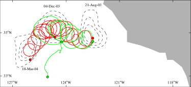
Figure 1: Trajectories of two RAFOS floats (red and green curves) and selected snapshots of a westward propagating bulge of the satellite altimetric sea surface height (SSH) field (dashed curves indicate selected isolines) in the southeastern North Pacific. The dots indicate the positions of the floats on the dates that the SSH bulge is shown.

Even more puzzling is that the two floats actually initially lie, as we show below, within the same coherent Lagrangian eddy (Beron-Vera et al., 2013; Haller and Beron-Vera, 2013, 2014). Representing an elliptic Lagrangian coherent structure (LCS; cf. Haller, 2014), the boundary of such an eddy defies the exponential stretching of typical material loops in turbulence. In effect, the eddy in question exhibits minimal filamentation and deformation over several months, and thus is expected to trap and carry within both floats.

The behavior of one of the floats supports this scenario and thus the altimetry-derived (i.e., geostrophic) upper-ocean current representation that sustains the coherent Lagrangian eddy. Ageostrophic processes of various types may be acting in the upper ocean, but these cannot explain the substantively different behavior of the other float. Indeed, ageostrophic effects cannot be so different on two initially nearby fluid particles in a region of mostly regular flow. Therefore, to resolve the puzzle, effects of a different class must be accounted for.

Here we argue theoretically, and show both numerically and observationally, that such effects can be produced by inertia, i.e., buoyancy and size finiteness. Inertial effects are commonly considered in atmospheric transport studies. These range from studies aimed at explaining observed motion of meteorological balloons (Paparella et al., 1997; Provenzale, 1999; Dvorkin, Paldor, and Basdevant, 2001) and spread of volcanic ash (Haszpra and Tél, 2011), to theoretical and numerical studies of particulate matter dispersal (Haller and Sapsis, 2008; Sapsis and Haller, 2009; Tang et al., 2009). In oceanography inertial effects have been also taken into account in several problems including sedimentation (Nielsen, 1994), and plankton sinking (Stommel, 1949), patchiness (Reigada et al., 2003) and selfpropulsion (Peng and Dabiri, 2009). However, they have been rarely considered in the motion of drifting buoys, macroscopic algae, or debris. To the best of our knowledge, their potential importance in influencing the motion of floats was only noted by Tanga and Provenzale (1994).

Our theoretical results reveal that while the boundary of a coherent Lagrangian eddy represents a transport barrier for fluid particles, it does not do so for inertial particles. Instead, a coherent Lagrangian eddy attracts or repels initially close inertial particles, depending on the particles’ density ratio with the ambient fluid and on the polarity (rotation sense) of the eddy.

We first validate these numerically using altimetry-derived currents in several regions of the ocean. Next, we use our findings to explain observed behavior in various ocean areas starting with the aforementioned floats, then proceeding with satellite-tracked surface drifting buoys (drifters), and finally macroscopic algae (Sargassum) distributions.

We emphasize that because our approach uses observationally-based velocity, it enables feature matching and analysis of specific measurements. Furthermore, our approach is self-consistent within the realm of incompressible two-dimensional flows. This is in marked contrast with a previous approach to surface ocean pattern formation (Zhong, Bracco, and Villareal, 2012), which considered passive advection by the surface velocity from a primitive-equation model (i.e., a truncation of the three-dimensional velocity). This is destined to create dissipative-looking patterns, but no actual passive tracer follows such a virtual velocity field.

We also note that our results are not applicable to the problem of accumulation of debris in subtropical gyres, which has been recently investigated by Froyland, Stuart, and van Sebille (2014) using probabilistic methods. The so-called great ocean garbage patches are produced by convergent wind-induced Ekman transport (Maximenko, Hafner, and Niiler, 2011). The Ekman dynamics governing basin-scale motions are very different than the quasigeostrophic dynamics governing mesoscale motions, our focus here. The former can produce dissipative patterns on the surface ocean by themselves, but the latter cannot unless inertial effects are taken into account, as we noted above and demonstrate below.

The remainder of the paper is organized as follows. Section 2.1 presents the mathematical setup required to formally introduce the coherent Lagrangian eddy notion, which is briefly reviewed in Section 2.2. The theoretical results relating to behavior of inertial particles near coherent Lagrangian eddies are presented in Section 2.3. In Section 2.4 further insight into inertial particle motion is provided. Numerical validation of the theoretical results is presented in Section 3. In Section 4 the theoretical results are used to explain observed behavior in the ocean. A summary and discussion is offered in Section 5. Finally, Appendix A includes details of the asymptotic analysis leading to our theoretical results, Appendix B is reserved for the description of the several datasets employed, and Appendix C gives some details of the various numerical computations performed.

II Theory

II.1 Mathematical setup

We consider an incompressible two-dimensional velocity field, $v(x,t)$, where position $x$ ranges on some open domain of $\mathbb{R}^{2}$ and time $t$ is defined on a finite interval. Specifically, we consider

$$v=\frac{g}{f}\nabla^{\perp}\eta,$$ (1)

where $\eta(x,t)$ is the SSH; the constants $f$ and $g$ stand for Coriolis parameter (twice the local vertical component of the Earth’s angular velocity) and acceleration of gravity, respectively; and $\perp$ represents a 90^∘-anticlockwise rotation. The velocity field (1) is representative of quasigeostrophic motions in the upper ocean, i.e., characterized by a small Rossby number, $\operatorname{Ro}:=V/L|f|$, where $L$ and $V$ are typical length and velocity scales, respectively. In particular, (1) is suitable to investigate transport near mesoscale eddies, our focus here. Fluid particles evolve according to

$$\dot{x}=v.$$ (2)

Let $F_{t_{0}}^{t}(x_{0}):=x(t;x_{0},t_{0})$ be the flow map that takes time $t_{0}$ positions to time $t$ positions of fluid particles obeying (2). An objective (i.e., frame-invariant) measure of material deformation in (2) is the right Cauchy–Green strain tensor,

$$C:=(\mathrm{D}F)^{\top}\mathrm{D}F,$$ (3)

where $\mathrm{D}$ stands for differentiation with respect to $x_{0}$. For any smooth $v$, $F$ represents a diffeomorphism, which ensures invertibility of $\mathrm{D}F$ and thus positive definiteness of $C$. Furthermore, incompressibility of $v$ implies $\det C=1$. Consequently, eigenvalues $\{\lambda_{i}\}$ and normalized eigenvectors $\{\xi_{i}\}$ of $C$ satisfy

$$0<\lambda_{1}\leq\lambda_{2}\equiv\frac{1}{\lambda_{1}},\quad\xi_{i}\cdot\xi_{j}=\delta_{ij}\quad i,j=1,2.$$ (4)

II.2 Coherent Lagrangian eddies

Haller and Beron-Vera (2013) seek elliptic LCS as material loops with small annular neighborhoods showing no leading-order variation in averaged material stretching (Fig. 2).

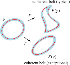
Figure 2: A closed material curve $\gamma$ (red) at time $t_{0}$ is advected by the flow into $F(\gamma)$ at time $t$. The advected curve remains coherent if a thin material belt around it (light blue) shows no leading-order variation in averaged stretching after advection.

Solving this variational problem reveals that elliptic LCS are uniformly stretching: any of their subsets are stretched by the same factor $\lambda$ under advection by the flow from time $t_{0}$ to time $t$. The time $t_{0}$ positions of $\lambda$-stretching elliptic LCS turn out to be limit cycles of one of the following two objective ODE for parametric curves $s\mapsto r(s)$:

$$r^{\prime}=\sqrt{\frac{\lambda_{2}-\lambda^{2}}{\lambda_{2}-\lambda_{1}}}\,\xi_{1}\pm\sqrt{\frac{\lambda^{2}-\lambda_{1}}{\lambda_{2}-\lambda_{1}}}\,\xi_{2},$$ (5)

where the prime stands for $s$ differentiation. More geometrically, limit cycles of (5) are closed null geodesics of the metric tensor $C-\lambda^{2}\mathrm{Id}$, which is Lorentzian in the domain satisfying $\lambda_{1}<\lambda^{2}<\lambda_{2}$. This provides a relativistic interpretation of coherent Lagrangian eddies (for details, cf. Haller and Beron-Vera, 2013, 2014).

The limit cycles of (5) will either grow or shrink under changes in $\lambda$, forming smooth annular regions of nonintersecting loops. The outermost member of such a band of coherent Lagrangian loops will be observed physically as the boundary of the coherent Lagrangian eddy. We refer to these maximal elliptic LCS as coherent Lagrangian eddy boundaries.

Limit cycles of (5) tend to exist only for $\lambda\approx 1$. Material loops characterized by $\lambda=1$ resist the universally observed material stretching in turbulence: they reassume their initial arclength at time $t$. This conservation of arclength, along with the conservation of the enclosed area in the incompressible case, creates extraordinary coherence for elliptic LCS.

II.3 Inertial effects near coherent Lagrangian eddies

The Maxey–Riley equation (Maxey and Riley, 1983) describes the motion of inertial (i.e., buoyant, finite-size) particles, which can deviate substantially from that of fluid (i.e., neutrally buoyant, infinitesimally-small) particles (cf. Cartwright et al., 2010). Here we consider a simplified version of the Maxey–Riley equation appropriate for inertial particle motion in a quasigeostrophic flow. We further derive a reduced form of this equation, which will allow us to assess behavior near a coherent Lagrangian eddy.

Specifically, ignoring added mass effects, the Basset history term, and so-called Faxen corrections, the Maxey–Riley equation for the motion of a small spherical particle in the flow produced by (1) is given by

$$\ddot{x}+f\dot{x}^{\perp}=\delta fv^{\perp}-\tau^{-1}\left(\dot{x}-v\right),$$ (6)

where the constants

$$\delta:=\frac{\rho}{\rho^{\mathrm{p}}},\quad\tau:=\frac{2a^{2}}{9\nu\delta}.$$ (7)

Here $\rho$ and $\nu$ are the fluid’s density and viscosity, respectively, and $\rho^{\mathrm{p}}$ and $a$ are the inertial particle’s density and radius, respectively. The left-hand-side of (6) is the inertial particle’s absolute acceleration. The first and second terms on the right-hand-side of (6) are the flow force and Stokes drag, respectively.

The simplified form of the Maxey–Riley equation (6) was priorly considered by Provenzale (1999) with the following differences. First, the fluid relative acceleration, $\rho(\partial_{t}v+v\cdot\nabla v)$, was included. This term is one order of magnitude smaller in Ro than $fv^{\perp}$ and thus is conveniently neglected here. Second, a centrifugal force term was included too, but this is actually balanced by the gravitational force on the horizontal plane. Third, a vertical buoyancy force term was considered, but this in the end played no role as the focus was on motion on a horizontal plane, as here.

We introduce the small nondimensional parameter:

$$\varepsilon:=\tau\frac{V}{L}=\frac{2}{9\delta}\left(\frac{a}{L}\right)^{2}\mathrm{Re}=\frac{\mathrm{St}}{\delta}\ll 1,$$ (8)

where $\mathrm{Re}$ and $\mathrm{St}$ are Reynolds and Stokes numbers, respectively. Consistent with the quasigeostrophic scaling assumptions leading to the fluid velocity field (1), we can set

$$\varepsilon=O(\operatorname{Ro}).$$ (9)

In Appendix A we show that inertial particle motion characterized by (9), e.g., the motion of particles much smaller than the typical lengthscale of the flow, is controlled at leading order by

$$\dot{x}=v^{\mathrm{p}}=v+\tau\left(\delta-1\right)fv^{\perp},$$ (10)

which is the reduced form of the Maxey–Riley equation we shall use. This reduced equation is valid up to an $O(\varepsilon^{2}$) error, after particles reach the vicinity of an attracting slow manifold exponentially fast.

Comparison of (2) and (10) reveals that the fluid velocity, $v$, and inertial particle velocity, $v^{\mathrm{p}}$, differ by a dissipative $O(\varepsilon)$ term. In the northern hemisphere ($f>0$) this term acts to deflect the motion of positively buoyant ($\delta>1$) finite-size or light particles to the left of the motion of fluid particles, while it acts to deflect the motion of negatively buoyant ($\delta<1$) finite-size or heavy particles to the right; in the southern hemisphere ($f<0$) it acts the opposite way (Fig. 3).

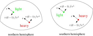
Figure 3: Velocity contributions to inertial particle’s velocity: light (heavy) particle motion deflects to the right (left) of fluid particle motion in the northern hemisphere and vice versa in the southern hemisphere.

Inertial effects, therefore, should promote divergence away from, or convergence into, coherent Lagrangian eddies when otherwise fluid particles circulate around them.

Specifically, let $\gamma$ be the boundary of a coherent Lagrangian eddy at time $t$ and $U_{\gamma}$ the region $\gamma$ encloses. Up to an $O(\varepsilon^{2})$ error, the flux across $\gamma$ is given by

$$\Phi_{\gamma} = \oint_{\gamma}\,(v-v^{\mathrm{p}})\cdot\mathrm{d}x^{\perp}$$ (11)

$$= \int_{U_{\gamma}}\nabla\cdot(v^{\mathrm{p}}-v)\,\mathrm{d}^{2}x$$

$$= \tau(1-\delta)f\int_{U_{\gamma}}\omega\,\mathrm{d}^{2}x,$$

where the loop integral is taken anticlockwise and $\omega:=-\nabla\cdot v^{\perp}(=gf^{-1}\nabla^{2}\eta)$ is the fluid’s vorticity. Inspection of expression (11) leads to the following conclusions:

1. cyclonic ($f\omega>0$) coherent Lagrangian eddies attract ($\Phi_{\gamma}<0$) light ($\delta>1$) particles and repel ($\Phi_{\gamma}>0$) heavy ($\delta<1$) particles; while

2. anticyclonic ($f\omega<0$) coherent Lagrangian eddies attract ($\Phi_{\gamma}<0$) heavy ($\delta<1$) particles and repel ($\Phi_{\gamma}>0$) light ($\delta>1$) particles.

Our results concerning heavy particles confirm the numerical observations of Provenzale (1999) and extend them to the behavior of light particles.

Our computations below are based on the reduced Maxey–Riley equation (10), which we refer to as the inertial equation. This follows the terminology of Haller and Sapsis (2008), who obtained the reduced form of a system similar to (6) in a nonrotating frame. Considering (10) is advantageous computationally and, as we will show, sufficiently accurate for the verification of our theoretical results.

II.4 Inertial Lagrangian Coherent Structures

While motion of inertial particles is not constrained by LCS, it is tied to analogous exceptional invariant curves referred to as inertial LCS (or iLCS; cf. Haller and Sapsis, 2008).

Of particular interest for our purposes here are hyperbolic iLCS of attracting type. These can be obtained by applying recent LCS theory results (Haller and Beron-Vera, 2012; Farazmand and Haller, 2013; Farazmand, Blazevski, and Haller, 2014; Haller, 2014) on system (10). Specifically, iLCS at time $t_{0}$ which attract nearby inertial particle trajectories over $[t_{0},t]$ are invariant curves $s\mapsto r(s)$ that satisfy

$$r^{\prime}=\xi^{\mathrm{p}}_{1}\quad\text{or}\quad r^{\prime}=\xi^{\mathrm{p}}_{2}$$ (12)

and

$$\sqrt{\smash[b]{\lambda^{\mathrm{p}}_{2}}}>1\quad\text{or}\quad\sqrt{\smash[b]{\lambda^{\mathrm{p}}_{1}}}<1$$ (13)

for $t<t_{0}$ or $t>t_{0}$, respectively. Here $\{\lambda_{i}^{\mathrm{p}}\}$ and $\{\xi_{i}^{\mathrm{p}}\}$ are eigenvalues and eigenvectors, respectively, of the Cauchy–Green tensor, $C^{\mathrm{p}}$, derived from system (10), which is an objective measure of deformation in that system. In forward time, segments of these invariant lines squeeze and stretch, respectively. As a result, they can be referred to as inertial squeezelines and inertial stretchlines, respectively. In a similar manner as the $\lambda$-lines discussed above, these invariant lines admit a null geodesic interpretation. In this case, the relevant Lorentzian metric tensor is given by $C^{\mathrm{p}}\Omega-\Omega C^{\mathrm{p}}$, where $\Omega$ is a 90^∘-anticlockwise rotation matrix (Farazmand, Blazevski, and Haller, 2014).

III Simulations

Here we present numerical results that confirm our theoretical predictions for the motion of inertial particles near coherent Lagrangian eddies in the ocean.

In each of our numerical tests a coherent Lagrangian eddy was detected assuming that fluid trajectories are governed by (2) with the velocity field given in (1); the SSH field is constructed using satellite altimetry measurements (Fu et al., 2010). All eddies were detected from 90-day forward integration and found to have $\lambda=1$. Successive positions of the boundaries of the eddies past the detection time were obtained from advection. Inertial particles were assumed to have $a=0.25$ m, which is a realistic radius value for commonly employed spherical drifting buoys. Both light and heavy particles were considered, with $\delta=1.1$ and $0.9$, respectively. These density ratio values are generally representative of surface floating and slowly or sinking buoys, respectively. For typical oceanic mesoscale eddies, with diameter $L\sim 150$ km and tangential velocity at the boundary $V\sim 0.1$ m s^-1, these inertial particle parameter choices give $\varepsilon\sim 0.01$. This $\varepsilon$ value turned out to be small enough for particle motion obeying the Maxey–Riley equation (6) to exhibit behavior qualitatively similar to that satisfying the inertial equation (6) employed in our simulations.

We begin by discussing the results of tests involving light and heavy particles initially located on the same position on the boundary of a coherent Lagrangian eddy. The results are summarized in Fig. 4, which consider a cyclonic (left panel) and an anticyclonic (right panel) eddy, both indicated in light blue. The eddy in the left panel is identifiable with an Agulhas ring, while that in the right panel with a cold-core Gulf Stream ring. The arclength of the boundary of each eddy on the detection date is reassumed 90 days after (recall that the eddies have $\lambda=1$). Coherence is nevertheless observed well beyond 90 days consistent with previous analyses of the satellite altimetry dataset (Beron-Vera et al., 2013; Haller and Beron-Vera, 2013). This is evident from the complete absence of filamentation. The light (green) and heavy (red) particles behave quite differently than the fluid particle (yellow) initially lying on the same position as the inertial particles on the boundary of each eddy. The fluid particle remains on all dates shown on the boundary of the Lagrangian eddy carrying the particle. Consistent with our predictions, the light (heavy) particle spirals out of (into) the Agulhas ring, while it spirals into (out of) the cold-core Gulf Stream ring.

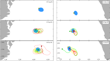
Figure 4: Simulated trajectories of light (green), heavy (red), and fluid (yellow) particles initially on the boundaries of two mesoscale coherent Lagrangian eddies (light blue) extracted from altimetry-derived velocity. Advection for the fluid particles is supplied by the altimetry-derived velocity, and heavy and light particle motion is controlled by the inertial equation (10). The eddies are identifiable with a cyclonic cold-core Gulf Stream ring (left panel) and an anticyclonic Agulhas ring (right panel).

We now provide more explicit support to our predictions by presenting the results from the computation of the pointwise flux of inertial particles across the boundary of a coherent Lagrangian eddy. Across a material loop $\gamma$, the pointwise flux of inertial particles is given by $(v^{\mathrm{p}}-v)\cdot n_{\gamma}$, where $n_{\gamma}$ is the outer unit normal to $\gamma$. Taking $\gamma$ as the boundary of the eddy identified above as an Agulhas ring, the latter is plotted in Fig. 5 on 24 November 2006 as a function of the boundary parameter $s$, chosen to be an azimuthal angle. The pointwise fluxes of light (solid green) and heavy (solid red) particles are everywhere inward and outward, respectively, along the boundary of the anticyclonic eddy in question. Thus our sign predictions for the total flux extend to the pointwise flux in this example.

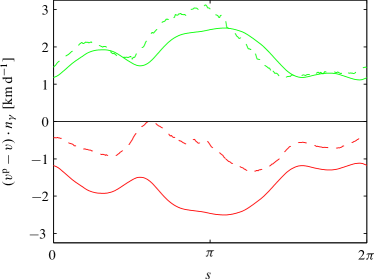
Figure 5: Pointwise flux on 24 November 2006 of simulated light (green) and heavy (red) particles across the boundary of the anticyclonic coherent Lagrangian eddy identified in the previous figure as an Agulhas ring. Solid and dashed curves correspond to simulations based on the inertial (10) and Maxey–Riley (6) equations, respectively.

We now turn to illustrate in Fig. 6 that the evolution of inertial particles is tied to attracting iLCS. This is done for patches of light (green) and heavy (red) particles lying initially outside the coherent Lagrangian Agulhas ring discussed above (light blue). Shown attracting iLCS (black) were computed as most stretching inertial stretchlines through each patch. This was done on the eddy detection time from a 90-day-forward integration. The evolution of each inertial stretchline was determined by advection. After experiencing substantial stretching the heavy particle patch is repelled away from the eddy. By contrast, the light particle patch spirals into the eddy. As expected, the attracting iLCS forms the centerpiece of the patch in each case. For completeness, the evolution of a fluid patch (yellow) is also shown. In this case, too, the patch evolution is tied to its centerpiece attracting LCS, computed also as the most stretching stretchline through patch. Consistent with the material nature of the boundary of the coherent eddy, the fluid patch spirals around the eddy without penetrating it.

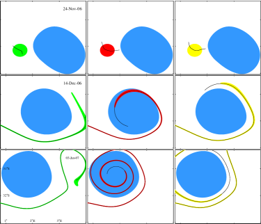
Figure 6: Simulated evolution of patches of light (green), heavy (red), and fluid (yellow) particles initially outside of the coherent Lagrangian Agulhas ring in the previous figures (light blue). Centerpiece attracting iLCS and LCS for the inertial and fluid particle patches, respectively, are indicated in black. Advection for fluid the particles is supplied by altimetry-derived velocities, and inertial particle motion is controlled by (10).

Finally, we show that for the parameters chosen, the qualitative behavior near a coherent Lagrangian eddy described by the Maxey–Riley (6) equation is captured by the inertial equation (10). This is illustrated in Fig. 5, where the dashed lines correspond to pointwise flux calculations based on the Maxey–Riley equation. This calculation involves trajectories started earlier, with a small (10% of the fluid velocity) perturbation to the velocity given in (10). While strict convergence of inertial- and Maxey–Riley-equation-based flux calculations has not been attained after 30 days of integration, both flux calculations agree in sign and share a similar structure. The slow convergence to the inertial manifolds arises from the highly unsteady nature of the altimetry-derived flow. Under such conditions, pronounced convergence is only observable near sufficiently persistent attracting sets. This is illustrated in Fig. 7, which shows trajectories of light (green) and heavy (red) particles lying on 24 November 2006 at the same position on the boundary of the coherent Lagrangian Agulhas ring considered in the pointwise flux calculations. As in Fig. 5, solid and dashed curves correspond to calculations based on inertial and Maxey–Riley equations, respectively. Once again, while details of inertial- and Maxey–Riley-equation-based trajectories are different and convergence can only be expected when particles are heavy, our predictions are seen to hold well: the heavy particle is attracted by the anticyclonic coherent Lagrangian eddy in question, whereas the light particle is repelled away from it.

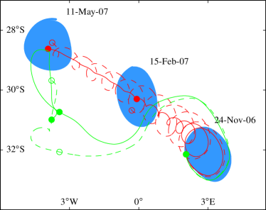
Figure 7: Simulated trajectories of light (green) and heavy (red) particles initially lying on the same location on the boundary of the coherent Lagrangian Agulhas ring of the previous figures (light blue) based on inertial (solid) and Maxey–Riley (dashed) equations.

IV Observations

In this section we discuss four sets of ocean observations that can be explained using our predictions for the motion of inertial particles near mesoscale coherent Lagrangian eddies.

The first set of observations, discussed in the Introduction, concern two RAFOS floats in the southeastern North Pacific. The floats took divergent trajectories despite their initial proximity within an anticyclonic mesoscale eddy. This eddy was revealed from the Eulerian footprints in the altimetric SSH field of a California Undercurrent eddy or “cuddy.” As we anticipated in the Introduction and now explicitly show in the top panel of Fig. 8, the altimetry-derived velocity field sustains a coherent Lagrangian eddy in nearly the same position as the SSH eddy. The eddy, obtained from a 90-day-forward integration with $\lambda=1$, is depicted (in light blue) on the detection date and two subsequent dates. The trajectory of each of the two floats is indicated by a curve, with their initial position highlighted by a dot. The divergent behavior of the float trajectories can be explained by inertial effects as follows. Note that the float indicated in green takes a slightly ascending trajectory (Fig. 8, bottom-left panel), whereas the float indicated in red takes a slightly descending trajectory (Fig. 8, bottom-right panel). Thus the ascending float represents a positively buoyant (i.e., light) object, whereas the descending float represents a negatively buoyant (i.e., heavy) object. The radius of the looping trajectory taken by the ascending float is seen to increase as the float drifts westward accompanying the anticyclonic coherent Lagrangian eddy revealed from altimetry, which is eventually abandoned by the float. This behavior adheres closely to what we have predicted for light particles. The radius of the looping trajectory taken by the descending float is not seen to decrease as the float drifts westward accompanying the eddy in question. However, in marked contrast with the ascending float, the descending float remains within this eddy. This behavior adheres to what we have predicted for heavy particles near anticyclonic coherent Lagrangian eddies.

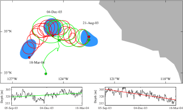
Figure 8: (top panel) Trajectories of the two RAFOS floats in Fig. 1 (green and red curves) and snapshots of an anticyclonic coherent material eddy detected from altimetry (light blue). The dots indicate the positions of the floats on the dates that the eddy is shown. (bottom-left panel) Depth of the green float as a function of time (black) with linear trend indicated (green). (bottom-right panel) As in the bottom-left panel, but for the red float.

The second set of observations concerns trajectories of satellite-tracked surface drifters deployed in the Gulf of Mexico ahead of hurricane Rita in September 2005. The drifters were deployed inside a Loop Current ring detected from its Eulerian footprints in the altimetric SSH field. A 30-day-forward integration of the altimetry-derived velocity field reveals that the anticyclonic SSH eddy contains a $\lambda=1$ coherent Lagrangian eddy with a radius of roughly 100 km, about 25-km smaller than that of the approximately circular area occupied by the SSH bulge. Figure 9 shows the coherent Lagrangian eddy (light blue) on the detection date and two subsequent positions obtained from advection. The trajectories of the drifters (a total of nine) are depicted in green (positions on the date shown are indicated by dots). Hurricane Rita made landfall about one week prior to the detection date, so neither the altimetry signal nor the motion of the drifters are affected by the high winds associated with this tropical cyclone system. Three drifters lie inside the eddy on the detection date, while the remaining six are located outside of the eddy, but close by its boundary. Overall, the drifters undergo growing looping trajectories. More than one month after the detection date, all nine drifters are found away from the center of the eddy, with three lying on its border and six lying well away from it. Noting that the drifters maintain afloat on the ocean surface, this behavior can be expected, given that anticyclonic coherent Lagrangian eddies repel away light particles according to our results.

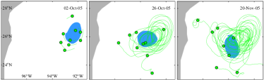
Figure 9: Trajectories of satellite-tracked surface drifters (green curves) and snapshots of a coherent Lagrangian Loop Current ring detected from altimetry (light blue). The dots indicate the positions of the drifters on the corresponding date.

The third set of observations involves the trajectory of a surface drifters tracked by the Argos satellite system, which was deployed inside an Agulhas ring, named Astrid, as part of the Mixing of Agulhas Rings Experiment (MARE) (van Aken et al., 2003). (Two additional drifters were deployed during MARE whose trajectories have not been possible to access. However, all three drifters behave similarly as it can be seen in Fig. 6 of van Aken et al. (2003).) Detected from its Eulerian footprints in the altimetric SSH field, ring Astrid was subjected to a detailed survey. Hydrographic casts across ring Astrid indicated the presence of a warm and saline core. Acoustic Doppler current profiling revealed that Astrid had, in addition to the baroclinic flow around its core, a significant barotropic component. A 30-day forward integration of the altimetry-derived velocity field reveals a coherent Lagrangian eddy with $\lambda=1$. This eddy has a mean radius of roughly 100 km, about half that of the approximately circular region spanned by the SSH bulge. Figure 10 shows selected snapshots of the coherent Lagrangian eddy (light blue) on three dates starting from the detection date. The trajectory of the Argos-tracked surface drifter is indicated in green (dots indicate the positions of the drifter on the corresponding dates). The drifter is seen to develop counterclockwise looping trajectories. This grows in radius and quite quickly the drifters abandon the vicinity of the eddy. The coherent Lagrangian eddy is rather short lived, thereby not revealing the presence of a well-developed Agulhas ring (possibly consistent with the lack of a well-defined core in the in-situ velocity measurements). However, over the lifespan of the eddy, the drifters’ behavior is consistent with our predictions for a light particle. Therefore, our results offer an explanation for its motion.

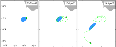
Figure 10: Trajectory of an Argos-tracked surface drifter (green curve) and snapshots of a short-lived coherent Lagrangian Agulhas ring detected from altimetry (light blue). A dot indicates the position of the drifter on the corresponding date.

Finally, the fourth set of observations involves distribution of floating Sargassum on the sea surface in the western North Atlantic inferred from the Medium Resolution Imaging Spectrometer (MERIS) aboard Envisat (Fig. 11, top panel). Sargassum corresponds to Maximum Chlorophyll Index (MCI) values exceeding $-0.25$ mW m^-2 sr^-1 nm^-1. Detected on 4 October 2006, the feature of interest takes a spiraled shape and lies inside a coherent Lagrangian cold-core Gulf Stream ring as revealed from altimetry. In the bottom-left panel of Fig. 11 the material boundary of this cyclonic coherent ring is shown overlaid on the Sargassum feature in question. This was obtained in Section 3 from advection of a coherent Lagrangian eddy boundary computed on 5 August 2006 from a 90-day-forward integration of the altimetry-derived velocity field (cf. Fig. 4, top-right panels). The accumulation of the floating Sargassum inside the Gulf Stream ring is consistent with the behavior of inertial particles near cyclonic coherent Lagrangian eddies, which attract light particles according to our results. The spiraled shape of the Sargassum distribution inside the ring is consistent too with the spiraled shape acquired by altimetry-based attracting light iLCS (parameters are as in Section 3). Selected iLCS are shown overlaid on the Sargassum distribution in the bottom-right panel of Fig. 11. These were obtained as backward-time light inertial squeezelines initialized along the boundary of the Gulf Stream ring on the date shown. The direction of the spiraling inertial particle motion along these iLCS is inward, as direct integration of the inertial particle equation reveals.

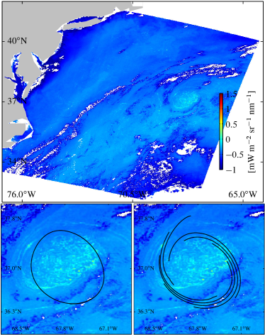
Figure 11: (top panel) Maximum Chlorophyll Index (MCI) in the western North Atlantic inferred from the Medium Resolution Imaging Spectrometer (MERIS) aboard Envisat on 4 October 2006. Floating Sargassum corresponds to MCI values in excess of $-0.25$ mW m^-2 sr^-1 nm^-1. (bottom-left panel) Boundary of a coherent Lagrangian cold-core Gulf Stream ring detected from altimetry (black) overlaid on the Sargassum distribution. (bottom-right panel) Altimetry-based attracting light iLCS (black) overlaid on the Sargassum distribution.

V Summary and discussion

In this paper we have provided an explanation for the observed tendency of drifting buoys and floating matter on the surface of the ocean to produce dissipative-looking patterns. This resolves an apparent paradox with the conservative-looking distributions that tracers passively advected by a rotating two-dimensional incompressible flow display. Our explanation takes into account inertial effects, i.e., those produced by the buoyancy and size finiteness of an object immersed in such a flow. These are described by a simplified Maxey–Riley equation consistent with a flow produced by a quasigeostrophic velocity where the pressure field is entirely due to differences in sea surface height. Because the latter are readily available from satellite altimetry measurements, our approach enables feature matching and analysis of specific observations. Furthermore, our approach is self-consistent within the realm of two-dimensional incompressible flows.

We have found that anticyclonic coherent Lagrangian eddies attract (repel) heavy (light) particles, while cyclonic ones behave the opposite way. We verified these results numerically using mesoscale SSH fields constructed from satellite altimetry measurements in various places of the ocean. Our findings also explained dissipative-type behavior shown by four sets of observations: divergent motion of subsurface floats initially inside a California Undercurrent eddy or “cuddy;” dispersion of surface drifters away from a Loop Current ring; ejection of surface drifters out of a well-studied Agulhas ring; and accumulation of sargassum inside of a cold-core Gulf Stream ring.

Beyond the reach of the Maxey–Riley description is motion of arbitrarily shaped objects; no known theory accounts for their effects. At the Maxey–Riley level there are terms and aspects that we have ignored which may contribute to narrow the gap between theory and observed motion. One such term is the memory term, but this only tends to slow down the inertial particle motion without changing its qualitative dynamics fundamentally (Daitche and Tél, 2011). Another neglected aspect is the dependence of fluid density on spatial position and time. Time varying density effects were investigated previously in idealized settings and found to be of importance (Tanga and Provenzale, 1994). The observational possibility to account for these effects is provided by satellite sensing of sea surface temperature and salinity. An additional aspect is the effect of submesosocale perturbations on the mesoscale motions of interest to us here. These may be of fully ageostrophic and possibly three-dimensional nature (McWilliams, 2008) or still be balanced to leading order, and thus essentially two-dimensional and incompressible (Klein and Lapeyre, 2009). The latter is particularly interesting as it opens the way to a potentially more accurate observationally-based velocity representation when high-resolution wide-swath altimetry becomes operational (Fu and Ferrari, 2009). The only observational improvement over altimetry-derived velocities may then be expected from the addition of an Ekman drift component estimated from satellite scattometer wind measurements. This typically small correction is regularly included, but in such a way as to match observed drifting buoy velocities (Lagerloef et al., 1999), which is not consistent with our inertial particle approach.

We finally note that a larger sample of drifting buoys and floating matter than that considered here is required to further validate our predictions, possibly improved by the consideration of fluid density variations and Ekman drift effects.

Appendix A Reduced Maxey–Riley equation

The second-order ODE (6) is equivalent to the following first-order ODE set:

$$\dot{x}=v^{\mathrm{p}},\quad\dot{v}^{\mathrm{p}}=f(\delta v-v^{\mathrm{p}})^{\perp}+\tau^{-1}(v-v^{\mathrm{p}}).$$ (14)

Taking $L$ and $L/V$ as length and time scales, respectively, and making $\tau|f|=1$ so that $\varepsilon=\tau V/L=\operatorname{Ro}\ll 1$, the nondimensional form of (14) reads:

$$\dot{x}=v^{\mathrm{p}},\quad\varepsilon^{2}\dot{v}^{\mathrm{p}}=\operatorname{sign}\!f\varepsilon(\delta v-v^{\mathrm{p}})^{\perp}+v-v^{\mathrm{p}}.$$ (15)

Inspection of (15) reveals that $x$ is a slow variable that changes at $O(1)$ speed, while $v^{\mathrm{p}}$ is a fast variable varying at $O(\varepsilon^{-2})$ speed. Consequently, (15) represents a singular perturbation problem. To regularize it, we displace and rescale time as $\varepsilon^{-2}(t-t_{0})$. Denoting with a circle differentiation with respect to this fast time variable, (15) transforms into

$$\mathring{x}=\varepsilon^{2}v^{\mathrm{p}},\quad\mathring{v}^{\mathrm{p}}=\operatorname{sign}\!f\varepsilon(\delta v-v^{\mathrm{p}})^{\perp}+v-v^{\mathrm{p}},\quad\mathring{t}=\varepsilon^{2}.$$ (16)

The $\varepsilon=0$ limit of system (16) has a manifold of fixed points. This manifold is normally attracting, and hence survives for small $\varepsilon>0$ in the form

$$v^{\mathrm{p}}=v+\varepsilon v_{1}+O(\varepsilon^{2}).$$ (17)

Plugging this asymptotic series expansion into the right-hand-side equation of system (16) and equating $O(\varepsilon)$ terms, it follows that

$$v_{1}=\operatorname{sign}\!f(\delta-1)v^{\perp}.$$ (18)

Inserting this expression in the left-hand-side equation of system (16), the inertial equation (10) follows once dimensional variables are recovered.

Particle dynamics governed by the inertial equation (10) evolve, over the finite-time interval of interest, on a two-dimensional manifold, $\mathcal{M}_{\varepsilon}$, in the phase space with coordinates $(x,v^{\mathrm{p}},t)$. This manifold is often referred to as slow because (10) restricted to it is a slowly varying system of the form $\mathring{x}=\varepsilon^{2}v^{\mathrm{p}}|_{\mathcal{M}_{\varepsilon}}=\varepsilon^{2}v+\varepsilon^{3}v_{1}+O(\varepsilon^{4})$. As shown in Haller and Sapsis (2008), this slow manifold attracts all inertial particle motions exponentially.

Appendix B Data

The altimetric SSH data employed in this paper consist of background and perturbation components. The background SSH component is steady, given by a mean dynamic topography constructed from satellite altimetry data, in-situ measurements, and a geoid model (Rio and Hernandez, 2004). The perturbation SSH component is transient, given by altimetric SSH anomaly measurements provided weekly on a 0.25^∘-resolution longitude–latitude grid. This perturbation component is referenced to a 20-year (1993–2012) mean, obtained from the combined processing of data collected by altimeters on the constellation of available satellites (Le Traon, Nadal, and Ducet, 1998). Mean dynamic topography and altimetry data are distributed by AVISO at http://www.aviso.oceanobs.com.

The RAFOS float trajectory data belong to the extensive dataset constructed from float deployments in the California Undercurrent over the period 1992–2010 (Collins et al., 2013). Acoustically tracked, RAFOS floats are quasi-isobaric, with their density varying with ambient temperature changes as a result of differing thermal expansions of the glass hull and aluminum end cap of the floats (Rossby, Dorson, and Fontaine, 1986). As opposed to seawater parcels, the floats sink when they warm and rise when they cool (Swift and Riser, 1994). The specific floats considered in this paper are shallow (300 db) floats number 105 and 106, obtained from http://www.oc.nps.edu/npsRAFOS.

The surface drifters in the Loop Current ring were deployed from air by the 53rd Hurricane Hunter Squadron ahead of hurricane Rita. Equipped to monitor surface conditions, these drifters were of Minimet (drogue at 15 m) and ADOS (with a 100-m-long thermistor chain hanging below) types. The trajectories of these drifters are available from the NOAA Global Drifter Program at http://www.aoml.noaa.gov/phod/dac.

Three surface drifters were deployed in ring Astrid during the MARE-1 cruise. These were standard spherical WOCE/TOGA drifters, fitted with an 8-m-long holey sock drogue at 15 m, with their positions tracked using the Argos satellite system (Sybrandy and Niiler, 1991). The trajectories of these drifters are not available from any database. The trajectory of the drifter considered in this paper was digitalized from Fig. 4 of van Aken et al. (2003) and spline fitted. We have not been able to reliably digitalize from this figure the other two trajectories, which exhibit a qualitatively similar behavior.

Finally, the MERIS image shown in Fig. 11 is of L1b Maximum Chlorophyll Index (MCI), a spectrometer parameter traditionally used to detect and track Sargassum (Gower and King, 2008). MERIS imagery is available from ESA Earth Online at https://earth.esa.int/web/guest/data-access.

Appendix C Computational details

The flow maps associated with (2) and (10) were obtained from integration for initial positions on a regular 0.5-km-width grid covering the domain of interest. This was done using a stepsize-adapting fourth-order Runge–Kutta method with interpolations obtained using a cubic scheme. The derivative of the flow maps were computed using finite differences on an auxiliary 0.1-km-width grid of four points neighboring each point in the above grid. Integrations of (5) and (12) were carried out using the same method while enforcing a unique orientation for the corresponding vector fields at each integration step (recall that these are constructed from eigenvector fields, which are not globally orientated). Detailed algorithmic steps for the extraction of coherent Lagrangian eddies are outlined in Haller and Beron-Vera (2013). The numerical computation of attracting iLCS involves the same algorithmic steps as those for attracting LCS; these are outlined in Haller and Beron-Vera (2012) and Farazmand and Haller (2013).

References

- Beron-Vera et al. (2013) Beron-Vera, F. J., Wang, Y., Olascoaga, M. J., Goni, G. J., and Haller, G., “Objective detection of oceanic eddies and the Agulhas leakage,” J. Phys. Oceanogr. 43, 1426–1438 (2013).
- Cartwright et al. (2010) Cartwright, J. H. E., Feudel, U., Károlyi, G., de Moura, A., Piro, O., and Tél, T., “Dynamics of finite-size particles in chaotic fluid flows,” in Nonlinear Dynamics and Chaos: Advances and Perspectives, edited by M. Thiel et al. (Springer-Verlag Berlin Heidelberg, 2010) pp. 51–87.
- Chelton, Schlax, and Samelson (2011) Chelton, D. B., Schlax, M. G., and Samelson, R. M., “Global observations of nonlinear mesoscale eddies,” Prog. Oceanogr. 91, 167–216 (2011).
- Collins et al. (2013) Collins, C. A., Margolina, T., Rago, T. A., and Ivanov, L., “Looping RAFOS floats in the California Current System,” Deep-Sea Res. II 85, 42–61 (2013).
- Daitche and Tél (2011) Daitche, A. and Tél, T., “Memory effects are relevant for chaotic advection of inertial particles,” Phys. Rev. Lett. 107, 244501 (2011).
- Dvorkin, Paldor, and Basdevant (2001) Dvorkin, Y., Paldor, N., and Basdevant, C., “Reconstructing balloon trajectories in the tropical stratosphere with a hybrid model using analysed fields,” Q. J. R. Meteorol. Soc. 127, 975–988 (2001).
- Farazmand, Blazevski, and Haller (2014) Farazmand, M., Blazevski, D., and Haller, G., “Shearless transport barriers in unsteady two-dimensional flows and maps,” Physica D 278-279, 44–57 (2014).
- Farazmand and Haller (2013) Farazmand, M. and Haller, G., “Attracting and repelling Lagrangian coherent structures from a single computation,” Chaos 23, 023101 (2013).
- Froyland, Stuart, and van Sebille (2014) Froyland, G., Stuart, R. M., and van Sebille, E., “How well-connected is the surface of the global ocean?” Chaos 24, 033126 (2014).
- Fu et al. (2010) Fu, L. L., Chelton, D. B., Le Traon, P.-Y., and Morrow, R., “Eddy dynamics from satellite altimetry,” Oceanography 23, 14–25 (2010).
- Fu and Ferrari (2009) Fu, L.-L. and Ferrari, R., “Observing oceanic submesoscale processes from space,” Eos 89, 488–489 (2009).
- Garfield et al. (1999) Garfield, N., Collins, C. A., Paquette, R. G., and Carter, E., “Lagrangian exploration of the California Undercurrent, 1992–95,” J. Phys. Oceanogr. 29, 560–583 (1999).
- Gower and King (2008) Gower, J. and King, S., “Satellite images show the Movement of floating Sargassum in the Gulf of Mexico and Atlantic Ocean,” Available from Nature Precedings (http://hdl.handle.net/10101/npre.2008.1894.1) (2008).
- Haller (2014) Haller, G., “Lagrangian coherent structures,” Ann. Rev. F 47, 137–162 (2014).