Investigating signatures of cosmological time dilation in duration measures of prompt gamma-ray burst light curves

Abstract

We study the evolution with redshift of three measures of gamma-ray burst (GRB) duration ($T_{\rm 90}$, $T_{\rm 50}$ and $T_{\rm R45}$) in a fixed rest frame energy band for a sample of 232 Swift/BAT detected GRBs. Binning the data in redshift we demonstrate a trend of increasing duration with increasing redshift that can be modelled with a power-law for all three measures. Comparing redshift defined subsets of rest-frame duration reveals that the observed distributions of these durations are broadly consistent with cosmological time dilation. To ascertain if this is an instrumental effect, a similar analysis of Fermi/GBM data for the 57 bursts detected by both instruments is conducted, but inconclusive due to small number statistics. We then investigate under-populated regions of the duration redshift parameter space. We propose that the lack of low-redshift, long duration GRBs is a physical effect due to the sample being volume limited at such redshifts. However, we also find that the high-redshift, short duration region of parameter space suffers from censorship as any Swift GRB sample is fundamentally defined by trigger criteria determined in the observer frame energy band of Swift/BAT. As a result, we find that the significance of any evidence for cosmological time dilation in our sample of duration measures typically reduces to $<2\sigma$.

1 Introduction

Gamma-ray burst (GRB) prompt emission has been detected at high-energies for over 40 years (von Kienlin et al., 2014; Sakamoto et al., 2011; Kaneko et al., 2006; Frontera et al., 2009; Klebesadel et al., 1973). It is only in the last decade, however, that a significant fraction of detected GRBs have sufficient ground-based follow-up to obtain a redshift measurement. This is largely thanks to the Swift satellite (Gehrels et al., 2004), which combines the capabilities of its wide field Burst Alert Telescope (BAT; Barthelmy et al. 2005) with arcsecond positional accuracies of the X-Ray Telescope (XRT; Burrows et al. 2005). With these X-ray positions, ground-based facilities have been able to build a comprehensive sample of GRBs with associated redshift using both photometric and spectroscopy methods in the optical and near IR wavelength regimes (e.g. Hjorth et al. 2012).

Knowing the redshift associated with a GRB places strong constraints on many properties of the transient event. Indeed, it was the first GRB redshift that finally settled the debate regarding whether the transients were Galactic or cosmological in origin (Metzger et al., 1997). Even with ground-based telescopes dedicated to GRB follow-up, and target of opportunity (ToO) programmes in place on large aperture facilities, approximately two thirds of Swift GRBs do not have an associated redshift. Additionally, other high-energy instruments such as the Gamma-ray Burst Monitor (GBM; Meegan et al. 2009) on the Fermi satellite cannot provide burst locations with sufficient accuracy to allow narrow field ground-based facilities to obtain a redshift.

With such a large fraction of GRBs lacking redshift, searches within the high-energy prompt light curves for tracers of redshifts have been previously attempted. As GRBs occur at cosmological distances and share a common central engine, it might expected that a signature of cosmological time dilation would be measurable in these light curves. Previous studies have considered variability of the high-energy light curve (Reichart et al., 2001) and the time lag between the same morphological light curve structure being observed in different energy bands (Norris et al., 2000) as an indicator of intrinsic burst luminosity.

More recently, Zhang et al. (2013) have considered traditional measures of duration, $T_{\rm 90}$ and $T_{\rm 50}$ (Kouveliotou et al., 1993), of a sample of Swift/BAT GRBs in a fixed rest frame energy band. $T_{\rm 90}$ and $T_{\rm 50}$ are the intervals over which the central 90% and 50% of prompt fluence are accumulated, respectively. This approach differs from most attempted duration correlations, as other time dilation searches often consider a fixed energy band in the observer frame. Using cross correlation function (CCF) analyses, it has long been known that the typical GRB light curve evolves such that it becomes softer at later times (Ukwatta et al., 2012; Margutti et al., 2010; Norris, 2002; Norris et al., 2000). Measuring durations such as $T_{\rm 90}$ of the same GRB in different energy bands, with characteristic energy $E$, therefore produces a different value of that duration, where $T_{\rm 90}\propto E^{-0.4}$ (Norris et al., 1996).

Measuring durations of a sample of GRBs in an observer frame defined energy band therefore combines two redshift dependent effects. First is that of cosmological time dilation, which causes durations to increase by a factor of $\left(1+z\right)$ as redshift increases. Superimposed upon this is also the effect of sampling a different region of the rest frame spectrum of each GRB. Indeed, as $T_{\rm 90}\propto E^{-0.4}$, it is to be expected that an additional factor of $\left(1+z\right)^{-0.4}$ would affect any correlation with redshift, as this is required to ensure the same region of all rest frame spectra are being sampled. Thus, by measuring duration in an energy band that is fixed in the observer frame, as has traditionally been attempted, it is expected that $T_{\rm 90}\left(E_{\rm 1,obs}-E_{\rm 2,obs}\right)\propto\left(1+z\right)^{0.6}$. It is perhaps a combination of this weakness in the correlation strength of duration increasing with increasing redshift and the large intrinsic scatter in the GRB prompt duration distribution that has prevented a clear detection of a time dilation signature in observer frame properties.

By choosing an energy band defined in the rest frame, Zhang et al. (2013) remove the energy dependent effects, and thus sample the same part of the rest frame spectra of all GRBs in their sample. Using a rest frame defined energy band, the expected correlation only depends on cosmological time dilation, such that $T_{\rm 90}\left(E_{\rm 1,rest}/(1+z)-E_{\rm 2,rest}/(1+z)\right)\propto\left(1+z\right)$. With a standardised rest-frame energy band in hand, Zhang et al. (2013) then average across broad bins in redshift and study the evolution of this average $T_{\rm 90,mean}$. For a sample of 139 Swift/BAT GRBs, they find $T_{\rm 90,mean}=10.5\left(1+z_{\rm mean}\right)^{0.94\pm 0.26}$ with a Pearson correlation coefficient of $r~{}=~{}0.93$ and chance probability of $p=7\times 10^{-3}$. An index of this value is remarkably close to that expected from cosmological time dilation.

In previous work, Littlejohns et al. (2013) examined simulations of real Swift/BAT GRBs placed at redshifts higher than those they were observed at. This work showed that the measured duration of an individual GRB evolved with simulated redshift due to three effects. The first was the expected time dilation of features within the light curve. In addition to this, however, was the gradual loss of the final FRED pulse tail due to poorer signal-to-noise ratio, and eventually the complete loss of late time pulses. As such, if the distribution of intrinsic GRB durations were constant in the rest frame, the observed evolution of the duration distribution as a function of redshift may not be expected to follow a simple power-law.

Additionally, by conserving the energy range of the GRB within the source frame, each burst samples a different part of the Swift/BAT effective area curve. As Zhang et al. (2013) note, the effective area of the BAT instrument reduces rapidly at $E>100$ keV and $E<25$ keV. With a standard band of $140/\left(1+z\right)$–$350/\left(1+z\right)$ keV, this could affect the durations measured for GRBs with the highest and lowest redshifts. These GRBs play the most significant role in determining the value of power-law index fitted to $T_{\rm 90}$ as a function of redshift.

In this work we aim to investigate the origins of any potential duration correlations with redshift. In § 2 we detail the sample of GRBs used in this work and the algorithms used to calculate the durations analysed in this work. In § 3 we begin by comparing our results to those of Zhang et al. (2013) before extending their sample to include 93 more recent BAT light curves. We also attempt to verify if the observed durations are real and not due to instrumental effects, by analysing light curves from Fermi/GBM. In § 4 we then discuss potential sources for apparent relations between duration and redshift.

2 Data

In this work we made use of data from both the Swift/BAT and Fermi/GBM. In addition to this we required redshift measurements, which were obtained from the Swift archive (http://swift.gsfc.nasa.gov/archive/grb_table/).

Of the 863 Swift/BAT detected GRBs that occurred prior to 2014 April 24^th, 251 have redshifts available in the Swift archive. Our final sample of GRBs is reduced further when considering only long GRBs ($T_{\rm 90}\left(15-350~{}{\rm keV}\right)$ $\geqslant$ 2 seconds) bright enough to yield a measurable $T_{\rm 90}$ in the Zhang et al. (2013) $140/\left(1+z\right)$–$350/\left(1+z\right)$ keV band. When imposing these criteria, the final sample consisted of 232 long GRBs. Short GRBs are excluded in this study as they derive from a different progenitor population (Nakar, 2007). By definition, they are also short in duration ($T_{\rm 90}\left(15-350~{}{\rm keV}\right)<2$ seconds; Kouveliotou et al. 1993) and tend to have low measured redshifts due to the more rapid decay of their optical afterglows. Thus, the inclusion of short GRBs would artificially enhance the strength of any positive trend in duration as a function of redshift.

Of the 232 long GRBs selected, 89 also fulfil the 1 second peak photon flux criterion $F_{\rm pk}$ $\geqslant$ 2.6 photons.s^-1.cm^-2 as introduced in Salvaterra et al. (2012) and used in Zhang et al. (2013). This corresponds to an increase in sample size of 67% and 41% in the full and bright samples, respectively, when compared to Zhang et al. (2013). Finally, of these 232 GRBs, there were also Fermi/GBM data available for 57 GRBs.

Swift/BAT data were downloaded from the UK Swift Science Data Centre (UKSSDC; http://www.swift.ac.uk/swift_portal/). The data for each burst were then processed using the standard software batgrbproduct. This produced event lists, from which light curves in user-defined energy ranges could be calculated.

To produce Swift/BAT light curves in the $140/\left(1+z\right)$–$350/\left(1+z\right)$ keV energy range, we used the standard batbinevt routine, which creates background subtracted light curves normalised by the number of fully illuminated detectors at all times. In all instances light curves were binned at 64 ms.

Fermi/GBM data were downloaded from the online Fermi GRB catalogue. This provided event lists for each GRB in all of the 12 sodium iodide (NaI) detectors. To produce 64 ms light curves the detectors in which the GRB was brightest had to be selected. Typically three NaI detectors were used for each burst. For those bursts that occurred prior to 2012 July 11^th we used the detectors outlined in Table 7 of the second Fermi/GBM GRB catalogue (von Kienlin et al., 2014). For GRBs after this date that we inspected the GBM Trigger Quick-look Plot obtained from the online catalogue to determine which detectors to use.

Fermi/GBM light curves were produced using the event lists from the detectors in which the GRB was bright. Only counts arising from photons in the $140/\left(1+z\right)$–$350/\left(1+z\right)$ keV band were extracted. These were then summed to form a single 64 ms light curve. Periods of burst activity were identified using the getburstfit routine available from the Fermi Science Support Center. This routine fits pulse shaped Bayesian blocks to the light curve. Each pulse is the sum of two exponentials, as described in Norris et al. (2005).

A background was fitted to the region of the light curve prior to the first Bayesian block and after the last Bayesian block. We considered a constant, linear and quadratic background and minimised the $\chi^{2}$ fit statistic for all three models. These fit statistics were compared using an F-test, first between the constant and linear fit. If a linear term did not provide a 3$\sigma$ improvement to the background fit, the constant background was adopted. Otherwise, a second F-test between the quadratic and linear models was also performed. In this instance, if the quadratic model was found to offer a 3$\sigma$ improvement to the background fit, this was then adopted, otherwise the linear model was used. The statistically favoured background was then subtracted from the entire light curve.

2.1 Durations

Zhang et al. (2013) use the Bayesian blocks battblocks algorithm, supplied as part of the suite of standard Swift software, to find $T_{\rm 90}$ in the $140/\left(1+z\right)$–$350/\left(1+z\right)$ keV band. battblocks requires a standard light curve files as produced by the batbinevt routine.

In this work, we use the methodology described in Butler et al. (2007) to determine all durations ($T_{\rm 100}$, $T_{\rm 90}$, $T_{\rm 50}$ and $T_{\rm R45}$) for both Swift/BAT and Fermi/GBM light curves. $T_{\rm 90}$ and $T_{\rm 50}$ measure the central 90% and 50% of cumulated source counts, respectively (Kouveliotou et al., 1993), while $T_{\rm R45}$ is the total time spanned by the bins containing the brightest 45% of the GRB source counts (Reichart et al., 2001). Error estimates for $T_{\rm 90}$, $T_{\rm 50}$ and $T_{\rm R45}$ were obtained by performing a bootstrap Monte Carlo (Lupton, 1993) using the counts and associated errors of each light curve bin within $T_{\rm 100}$.

Figure 1: Comparison between observer frame $T_{\rm 90,obs}$ values derived in this work and those shown in Table 1 of Zhang et al. (2013). For each GRB light curves were extracted in the $140/\left(1+z\right)$–$350/\left(1+z\right)$ keV energy ranges. The dashed line denotes equality.

To ensure consistency with previous work, we compare the values of $T_{\rm 90}$ found in this work to those of Zhang et al. (2013). Generally, there is a good agreement between the two values. For approximately 5% of the population we recover a significantly longer value of $T_{\rm 90}$ than the battblocks value reported by Zhang et al. (2013). Visual inspection of these cases revealed three instances of precursors not detected by the battblocks algorithm, with the other light curves having a low flux extended emission tail. The battblocks routine is less sensitive to such emission tails as they do not conform to the expected Fast Rise Exponential Decay (FRED) pulse shape.

3 Analysis

3.1 Choosing an average

To uncover a signature of cosmological time dilation in burst durations, we first recreated the models outlined in Zhang et al. (2013). We began by binning the 139 burst sample considered in that work. In binning the data, Zhang et al. (2013) measure the mean redshift and mean $T_{\rm 90,obs}$ of the bursts within each bin, where $T_{\rm 90,obs}$ corresponds to $T_{\rm 90}$ in the observer frame. As the data are modelled with a power-law, we consider the arithmetic mean to be more sensitive to outliers within the bin than other averages. With this in mind, we also considered the median and geometric mean of $T_{\rm 90,obs}$ within each bin. The value of average redshift was calculated using the same method as $T_{\rm 90,obs}$ in all three instances. The bins obtained using these three types of average for the full Zhang et al. (2013) sample are shown in Figure 2.

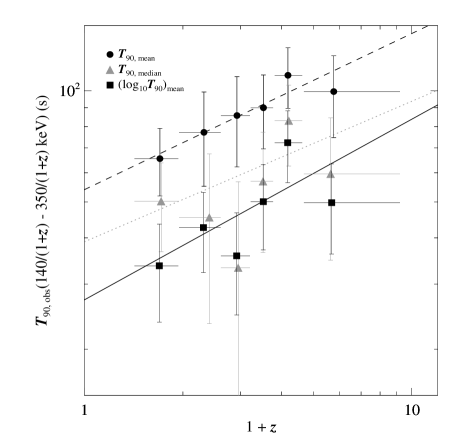
Figure 2: Fitted power-laws to observer frame $T_{\rm 90,mean}$, $T_{\rm 90,median}$ and $\left(\log_{10}T_{\rm 90}\right)_{\rm mean}$ for the full 139 GRB Zhang et al. (2013) sample. $T_{\rm 90,mean}$ bins are represented by black circles, $T_{\rm 90,median}$ bins are represented by grey triangles and $\left(\log_{10}T_{\rm 90}\right)_{\rm mean}$ bins are represented by black squares.

With average bins in hand, we then fitted power-laws to the data, as expected if the evolution in the $T_{\rm 90,obs}$ distribution arises purely from cosmological time dilation. To assess the quality of each fit we used the $\chi^{2}$ fit statistic, where the $\chi^{2}$ minimisation was undertaken in logarithmic space.

In Table 1 we detail eight alternative fits. When modelling average bins, we used the statistical scatter within each bin as an estimate of the error on each average. For the arithmetic mean and median, this scatter was calculated in linear space, whilst for the geometric mean the scatter in $\log_{10}\left(T_{\rm 90,obs}\right)$ was used.

The first three models in Table 1 correspond to the dashed lines in Figure 2 as denoted by the key. The power-law indices for all average methods under-predict that expected from cosmological time dilation, although the error on the power-law index in all three instances is large. The $\chi^{2}$ fit statistic also appears to be reasonable, although inspection of Figure 2 shows that this is a consequence of a large scatter in the $T_{\rm 90,obs}$ values within each bin leading to large errors associated with the average bins. This is particularly the case when using the median to average the values within each bin. Further inspection of Figure 2 reveals that the median average does not conform well to the modelled power-law.

We next recreated the Zhang et al. (2013) fit to the individual bright GRBs. This subset of bursts is identified by imposing a brightness threshold on the sample. As with Zhang et al. (2013) we apply a threshold of $F_{\rm pk}\geqslant 2.6$ photons.s^-1.cm^-2 (Salvaterra et al., 2012), where $F_{\rm pk}$ is the one second peak photon flux. This bright subset is shown in Figure 3.

Figure 3: $T_{\rm 90,obs}$ in the $140/\left(1+z\right)$–$350/\left(1+z\right)$ keV band as a function of redshift for the 63 GRBs defined in the Zhang et al. (2013) bright sample. The dashed line is the Zhang et al. (2013) power-law fit to each individual GRB, when all bursts are considered to have equal fractional errors, $\left(\Delta T_{\rm 90,obs}/T_{\rm 90,obs}\right)=\left(1/\ln 10\right)$, not including the measurement error determined by our $T_{\rm 90}$ routine.

We attempted to model the bright Zhang et al. (2013) sample first by considering the error in each burst to be that reported by the Butler et al. (2007) $T_{\rm 90}$ algorithm. This did not agree with the model fit in Zhang et al. (2013), so we repeated the fitting, this time applying a constant fractional error of $\left(\Delta T_{\rm 90,obs}/T_{\rm 90,obs}\right)=1/\ln\left(10\right)$ to every point. The model parameters and associated errors obtained with this latter fit corresponds to the values reported by Zhang et al. (2013).

In Figure 3 we show the fit obtained by Zhang et al. (2013). Due to the selected value of constant error for all of the data, the $\chi^{2}$ fit statistic for this model appears reasonable. However, Figure 3 clearly shows that the scatter in the distribution of $T_{\rm 90,obs}$ is large and not accounted for by the power-law fit. The poor nature of the fit is more clear when considering the fit statistic obtained when using the true measured error in each $T_{\rm 90,obs}$.

As with the full 139 burst sample, we also binned the bright GRB sample from Zhang et al. (2013). We again fitted power-laws to the arithmetic mean, median and geometric mean of $T_{\rm 90,obs}$ for the bright subset of GRBs, as shown in the bottom three rows of Table 1. The values of power-law index obtained for the bright subset are consistent, within error, with those obtained for the full sample, although in all three cases are steeper for the bright GRB sample. We note, however, that $\chi/\nu^{2}$ $<$ 1, which indicates that the statistical error for each bin is large, meaning the power-law fit is not strongly constrained in each case.

Table 1: Details of fits to $T_{\rm 90,obs}$ as a function of $1+z$ for the original bright and full GRB samples described in Zhang et al. (2013). The top three rows describe the models of the full sample weighting each bin by its statistical error on the bin (see Figure 2). The next two rows are for the bright sample with each burst fitted individually. The final three rows are for average bins of the bright sample, using statistical error to weight each bin. $\log_{10}N$ is the logarithm of the fitted normalisation of each power-low.

Sample	Average	Error	$\log_{10}N$	Index	$\chi^{2}/\nu$
All	Arithmetic mean	$\sigma_{\rm bin}/{\rm SE}_{\rm bin}$	1.73 $\pm$0.05	0.42 $\pm$0.09	0.64/4
All	Median	$\sigma_{\rm bin}/{\rm SE}_{\rm bin}$	1.59 $\pm$0.12	0.38 $\pm$0.23	1.94/4
All	Geometric mean	$\sigma_{\rm bin}/{\rm SE}_{\rm bin}$	1.43 $\pm$0.13	0.49 $\pm$0.25	3.13/4
Bright	None	$T_{\rm 90,obs}/\ln\left(10\right)$	1.25 $\pm$0.20	0.58 $\pm$0.45	87.76/59
Bright	None	$\Delta T_{\rm 90}$	1.89 $\pm$0.09	-0.51 $\pm$0.21	70608.81/59
Bright	Arithmetic mean	$\sigma_{\rm bin}/{\rm SE}_{\rm bin}$	1.48 $\pm$0.10	0.66 $\pm$0.23	1.04/4
Bright	Median	$\sigma_{\rm bin}/{\rm SE}_{\rm bin}$	1.31 $\pm$0.18	0.76 $\pm$0.43	1.27/4
Bright	Geometric mean	$\sigma_{\rm bin}/{\rm SE}_{\rm bin}$	1.20 $\pm$0.15	0.72 $\pm$0.33	1.88/4

For all further fitting in this work, we have chosen to only fit to binned data. As we are fitting a power-law in logarithmic space, we adopt the geometric mean and weight all average bins by the scatter in $\log_{10}\left(T_{\rm 90,obs}\right)$.

3.2 Updating the Swift/BAT sample

The original Zhang et al. (2013) sample contains GRBs with a known redshift detected by 2012 March. We extended this sample by considering all bursts detected up to 2014 April 23^rd. This gave us an initial list of 251 Swift detected GRBs with redshift. Using our $T_{\rm 90}$ algorithm we found only 238 GRBs had a measurable $T_{\rm 90,obs}\left(140/\left(1+z\right)-350/\left(1+z\right)~{}{\rm keV}\right)$. Additionally, 6 of these GRBs were short ($T_{\rm 90,obs}\left(15-350~{}{\rm keV}\right)<2$ s), so we removed them from the extended sample. Imposing the $F_{\rm pk}$ brightness threshold (Salvaterra et al., 2012) on this increased subset yielded an extended bright sample of 89 GRBs.

Having determined the full and bright samples to be fitted, we considered $T_{\rm 90,obs}$, $T_{\rm 50,obs}$ and $T_{\rm R45,obs}$ for all bursts. The full distributions of all three are shown as a function of redshift in Figure 4, where the grey points are individual GRBs and the black points are average bins obtained using the geometric average of durations and redshifts within each bin.

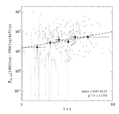
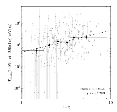
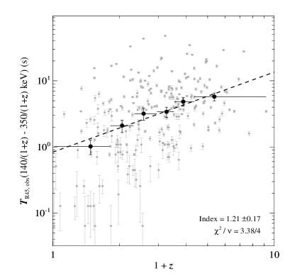
Figure 4: $T_{\rm 90,obs}$, $T_{\rm 50,obs}$ and $T_{\rm R45,obs}$ obtained in the $140/\left(1+z\right)$–$350/\left(1+z\right)$ keV energy range for the 232 GRBs in the full Swift/BAT sample. Grey points correspond to the individual GRBs, while black points are the geometric average. In each panel the bins represented by the black average points contain the same GRBs. The black dashed line corresponds to the best fit power-law obtained when modelling binned data. The $\chi^{2}$ fit statistic, degrees of freedom and power-law index obtained are indicated in each panel.

The three panels in Figure 4 show that, for all three duration measures, the average duration tends to increase with redshift. The final average bin of each duration measure does not conform to this trend, however. The fits shown in each of the panels are also detailed in Table 2, alongside modelling of the bright subset for all three durations.

Table 2: Details of fits to geometric average of duration as a function of $\left(1+z\right)$ for the extended bright and full GRB samples. $N_{\rm GRBs}$ is the total number of bursts contained in each fit, while $\log_{10}N$ is the logarithm of the normalisation to each fitted power-law.

Sample	Duration	$N_{\rm GRBs}$	$\log_{10}N$	Index	$\chi^{2}/\nu$
All	$T_{\rm 90,obs}$	232	1.17 $\pm$0.13	0.83 $\pm$0.23	3.37/4
All	$T_{\rm 50,obs}$	232	0.66 $\pm$0.11	1.01 $\pm$0.20	2.78/4
All	$T_{\rm RT45,obs}$	232	0.08 $\pm$0.09	1.21 $\pm$0.17	3.38/4
Bright	$T_{\rm 90,obs}$	89	1.23 $\pm$0.17	0.64 $\pm$0.36	3.14/4
Bright	$T_{\rm 50,obs}$	89	0.65 $\pm$0.14	0.77 $\pm$0.30	2.54/4
Bright	$T_{\rm RT45,obs}$	89	0.32 $\pm$0.17	0.70 $\pm$0.37	5.83/4

For all three durations, the behaviour of the geometric average as a function of redshift can be fairly well described by a power-law. In all three cases, however, the final average bin is over-predicted by the fitted power-law model.

Of the three duration measures, $T_{\rm 50,obs}\left(140/\left(1+z\right)-350/\left(1+z\right)~{}{\rm keV}\right)$ has the lowest $\chi^{2}$ value, and also has a value most consistent with that expected from time-dilation. Care must be taken, though, as the $\chi^{2}$ fit statistic indicates that the quality of this fit is dominated by the statistical scatter of individual $T_{\rm 50,obs}\left(140/\left(1+z\right)-350/\left(1+z\right)~{}{\rm keV}\right)$ values within the bin.

As shown in Littlejohns et al. (2013), at high redshifts, difficulties arise in recovering periods of late-time pulse morphology due to a decreasing signal-to-noise ratio in the pulse tail. $T_{\rm 90}$ probes the extended tail of prompt emission more deeply than $T_{\rm 50}$, and so should be more sensitive to these effects. As such, if the distribution of rest frame GRB durations is indeed constant, then $T_{\rm 50,obs}$ might be expected to most clearly exhibit the effects of cosmological time dilation. This is what is seen in Figure 4, with the power-law fitted to the geometric average $T_{\rm 50,obs}$ as a function of redshift is closest to $\left(1+z\right)^{1}$.

Table 2 also indicates that restricting the sample to only the brightest bursts results in a slightly shallower power-law index. With the exception of $T_{\rm R45,obs}$, this difference between the bright and full samples for all three durations is not, however, greater than the error associated with the power-law index in either fit.

We noted in Figure 4 that there are several GRBs where $\Delta T_{\rm 90,obs}$ is comparable to, or exceeds, the measured value of $T_{\rm 90,obs}$. We therefore re-fitted both the full and bright updated Swift/BAT sample excluding all GRBs where $\Delta T_{\rm 90,obs}>T_{\rm 90,obs}$. This reduced the sample sizes to 220 and 84, respectively. When filtering the data in this way, the GRBs that were removed tended to be in the low redshift, low duration regions of our parameter space. Table 3 details the fitted power-laws to the geometric mean average bins for each duration after the data had been filtered.

Table 3: Details of fits to geometric average of duration as a function of $\left(1+z\right)$ for the filtered extended bright and full GRB samples. $N_{\rm GRBs}$ is the total number of bursts considered in each fit, while $\log_{10}N$ is the logarithm of the normalisation to each fitted power-law.

Sample	Duration	$N_{\rm GRBs}$	$\log_{10}N$	Index	$\chi^{2}/\nu$
All	$T_{\rm 90,obs}$	220	1.39 $\pm$0.12	0.51 $\pm$0.23	4.16/4
All	$T_{\rm 50,obs}$	220	0.87 $\pm$0.08	0.69 $\pm$0.16	2.04/4
All	$T_{\rm RT45,obs}$	220	0.08 $\pm$0.09	1.01 $\pm$0.18	4.26/4
Bright	$T_{\rm 90,obs}$	84	1.37 $\pm$0.22	0.40 $\pm$0.49	6.20/4
Bright	$T_{\rm 50,obs}$	84	0.81 $\pm$0.21	0.47 $\pm$0.48	7.70/4
Bright	$T_{\rm RT45,obs}$	84	0.42 $\pm$0.17	0.53 $\pm$0.37	7.88/4

In all instances, as shown in Tables 2 and 3, the power-law index decreases when removing those bursts with large relative uncertainties in $T_{\rm 90,obs}$. Comparing these new values with that expected from cosmological time dilation, we find that only $T_{\rm R45,obs}$ now is consistent with this hypothesis. However, it is important to note that when sampling only the brightest bursts, as defined by Zhang et al. (2013), the correlation of $T_{\rm R45,obs}$ with redshift is shallower and is more poorly described by a power-law.

Removing bursts with greater relative uncertainty in $T_{\rm 90,obs}$ demonstrates that care must be taken when defining the sample over which any of these putative correlations are to be measured. In this instance, the correlations favour fitted values more consistent with cosmological time dilation when also considering GRBs with poorly defined values of duration.

Modelling the evolution of redshift in the manner described above allows us to compare the geometric average value of a duration measure as a function of redshift, however, it does not provide information regarding the shape of the distribution. We therefore compared subsets of the duration distributions, defined by redshift.

We calculated the rest frame values of $T_{\rm 90,obs}$, $T_{\rm 50,obs}$ and $T_{\rm R45,obs}$ (where e.g. $T_{\rm 90,rest}=T_{\rm 90,obs}/\left(1+z\right)$), which correspond to being measured in the 140–350 keV range of the rest frame of each GRB. We then isolated four subsets within the full extended sample: those with a redshift above the median redshift of the sample, $z_{\rm median}=1.95$; those with $z<z_{\rm median}$; GRBs with redshift in the upper quartile of the sample distribution and finally GRBs with a redshift in the lower quartile of the sample distribution.

We then performed a Student’s $t$-test comparing GRBs with $z>z_{\rm median}$ to those with $z<z_{\rm median}$ for each duration measure. As the duration measures are best represented in logarithmic space, these Student’s $t$-tests were performed using $\log_{10}\left(T_{\rm dur,rest}\right)$, where $T_{\rm dur,rest}$ was $T_{\rm 90,rest}$, $T_{\rm 50,rest}$ or $T_{\rm R45,rest}$. We also compared the duration of bursts with redshift in the upper quartile to the durations of bursts with redshifts in the lower quartile. The distributions of rest frame durations are shown in Figure 5. The results for each $t$-test are detailed in Table 4.

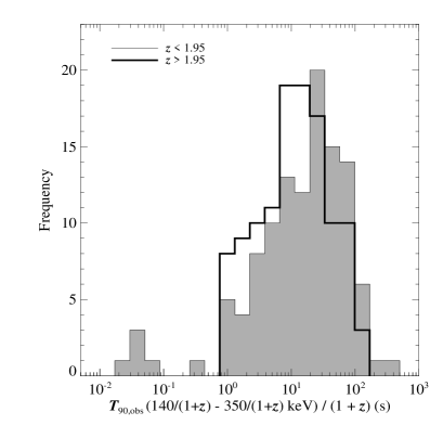
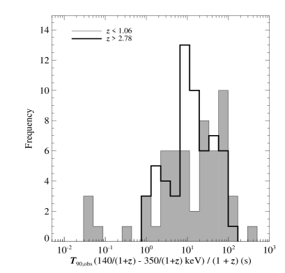
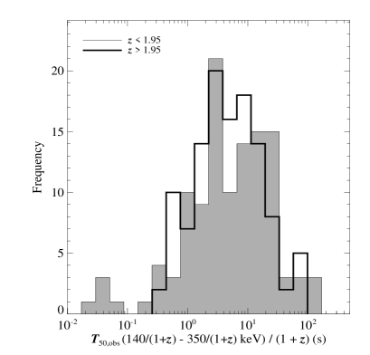
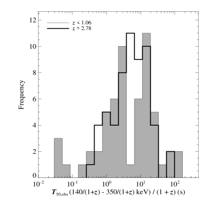
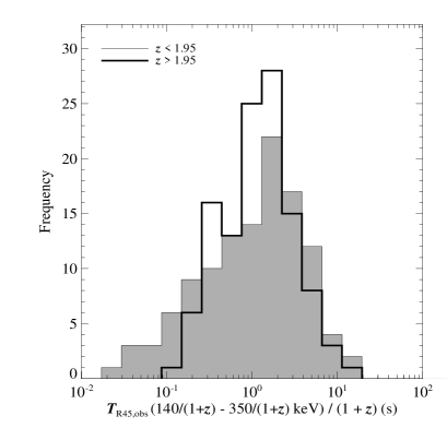
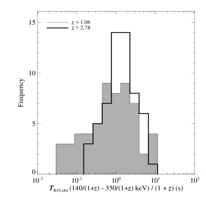
Figure 5: Histograms comparing rest frame $\left(140~{}-~{}350~{}{\rm keV}\right)$ durations for sub-samples of the GRB population. The left panels compare the 116 GRBs with $z<z_{\rm median}$ to the 116 with $z>z_{\rm median}$. The right hand panel compares the 58 bursts in the lowest redshift quartile to the 58 GRBs in the highest redshift quartile. The top panels are comparisons of $T_{\rm 90,rest}$, the middle two panels are $T_{\rm 50,rest}$ and the bottom two are $T_{\rm R45,rest}$.

Table 4: Results from Student’s $t$-tests comparing rest frame duration measures. $N_{1}$ and $N_{2}$ give the number of GRBs in each subset, $z_{1}$ and $z_{2}$ detail the redshift limits for each distribution. $t$ is the Student’s $t$-test statistic and $p\left(H_{0}\right)$ is the probability that the two distributions have the same mean.

Duration	$N_{1}$	$N_{2}$	$z_{1}$	$z_{2}$	$t$	$p\left(H_{0}\right)$
$T_{\rm 90,rest}$	116	116	$<$1.95	$>$1.95	0.81	0.42
$T_{\rm 50,rest}$	116	116	$<$1.95	$>$1.95	0.15	0.88
$T_{\rm R45,rest}$	116	116	$<$1.95	$>$1.95	-1.11	0.27
$T_{\rm 90,rest}$	58	58	$<$1.06	$>$2.78	-0.22	0.82
$T_{\rm 50,rest}$	58	58	$<$1.06	$>$2.78	-0.70	0.47
$T_{\rm R45,rest}$	58	58	$<$1.06	$>$2.78	-2.47	0.01

From Figure 5 and Table 4 it can be seen that for five of the six statistical tests, there is no significant difference between the populations being compared. This supports the claims of Zhang et al. (2013) that the distributions of prompt emission rest frame durations in a rest frame defined energy band are constant.

The results of the test comparing those values of $T_{\rm R45,rest}$ in the lower redshift quartile to those in the upper redshift quartile, however, indicate a difference in the distribution at a significance of approximately 3$\sigma$. The sixth panel of Figure 5 shows this is because the distribution at higher redshifts appears to be narrower and, in particular, lacks low values of $T_{\rm R45,rest}$. It is worth noting, as shown in Figure 4 that these low duration values of $T_{\rm R45,obs}$ have higher measured errors, indicating a greater uncertainty in these values.

$T_{\rm R45,obs}$ fundamentally differs from $T_{\rm 90,obs}$ and $T_{\rm 50,obs}$, as the former probes only the brightest region of prompt emission. As such, $T_{\rm R45,obs}$ is more insensitive to the presence quiescent periods of a light curve. Conversely, should a quiescent period occur within the central 50% of GRB high-energy fluence, both $T_{\rm 90,obs}$ and $T_{\rm 50,obs}$ would include that period. It is perhaps expected, therefore, that $T_{\rm R45,obs}$ is less likely to exhibit evidence of cosmological time dilation.

While most pronounced in the $T_{\rm R45}$ distributions, $T_{\rm 90,rest}$ and $T_{\rm 50,rest}$ also show a small population of low duration, low redshift bursts. It is possible that these are fainter GRBs, and as such cannot be detected by the Swift/BAT at higher redshifts. This effect is investigated in more detail in § 4.2.

3.3 Durations measured by Fermi/GBM

By extracting durations in a rest frame defined energy range, the observer energy range is a function of redshift. As such, detector effects may inhomogeneously alter the recovered durations of the sample. To test whether such effects are present, we also cross-referenced the 232 GRBs in our extended sample with those observed by Fermi/GBM. This yielded 57 GRBs for which a Swift/BAT light curve, Fermi/GBM light curves and redshift measurement were available.

The Fermi/GBM $140/\left(1+z\right)$–$350/\left(1+z\right)$ keV light curves were extracted for each GRB. We then binned the light curves using the methodology discussed in § 3.1. We also took the Swift/BAT light curves for only this subset of 57 GRBs to ensure these burst durations were representative of the larger Swift/BAT sample.

Figure 6 shows the individual duration measures obtained from both the Swift/BAT and Fermi/GBM light curves in grey. Also shown in black are the geometric averages as a function of redshift. The binning of GRBs is identical in all six panels. Details of the fitted power-laws are given in Table 5.

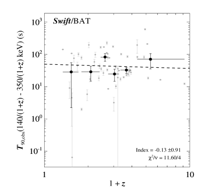
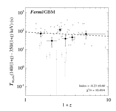
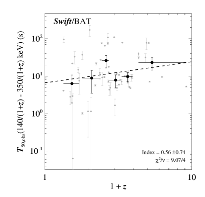
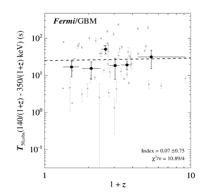
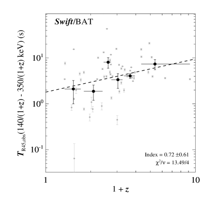
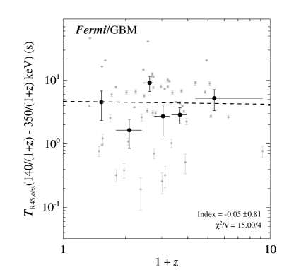
Figure 6: $T_{\rm 90,obs}$, $T_{\rm 50,obs}$ and $T_{\rm R45,obs}$ obtained in the $140/\left(1+z\right)$–$350/\left(1+z\right)$ keV energy range for the 57 GRBs in the joint Swift/BAT-Fermi/GBM sample. Grey points correspond to the individual GRBs, while black points are the geometric average. Swift/BAT data are shown in the left-hand column, while the corresponding Fermi/GBM data are shown in the right column. Binning of GRBs is identical in all six panels. The black dashed line in each panel corresponds to a power-law fitted to the average bins. The $\chi^{2}$ fit statistics, degrees of freedom and power-law indices of all six models are indicated in each panel.

Table 5: Fitted power-law parameters and fit statistics for the 57 GRB joint Swift/BAT-Fermi/GBM subset. For each fit, the duration considered and instrument from which light curves were taken are shown. $\log_{10}N$ is the logarithm of the normalisation to each fitted power-law.

Instrument	Duration	$\log_{10}N$	Index	$\chi^{2}/\nu$
Swift/BAT	$T_{\rm 90,obs}$	1.70 $\pm$0.47	-0.13 $\pm$0.91	11.60/4
Swift/BAT	$T_{\rm 50,obs}$	0.82 $\pm$0.40	0.56 $\pm$0.74	9.07/4
Swift/BAT	$T_{\rm R45,obs}$	0.26 $\pm$0.34	0.72 $\pm$0.61	13.49/4
Fermi/GBM	$T_{\rm 90,obs}$	1.95 $\pm$0.27	-0.23 $\pm$0.60	10.49/4
Fermi/GBM	$T_{\rm 50,obs}$	1.40 $\pm$0.36	0.07 $\pm$0.75	10.89/4
Fermi/GBM	$T_{\rm R45,obs}$	0.67 $\pm$0.41	-0.05 $\pm$0.81	15.00/4

Figure 6 appears to show that the geometric averages of all three duration measures are less positively correlated with redshift when calculated for the same sample using Fermi/GBM light curves. Inspection of Figure 6 reveals the duration distributions for both instruments differ most significantly at low redshifts.

However, with a large intrinsic scatter in the duration distributions, the geometric average bins are less well represented by a power-law model fit. Due to the large scatter of duration values within each bin the statistical errors of these bins, and subsequently the model fit parameters, are large. The differences in power-law index fitted to all three duration distributions is approximately the same size as the error in the fitted parameter. This indicates a larger sample of Fermi/GBM GRBs with measured redshift is required to assess the significance of this difference. Comparisons between Tables 3 and 5 also show that a larger sample is required to be more representative of the full Swift/BAT sample and remove the effects of small number statistics.

4 Discussion

4.1 Low-redshift long-duration GRBs

There are two regions of the redshift-duration parameter space that, if artificially underpopulated, would enhance a correlation between the two quantities. The first is at low redshifts, but long durations. At low-redshifts, the sample of observed GRBs is volume limited. The observed GRB sample should therefore reflect the most common type of burst within the total distribution.

A volume limited sample of GRBs should also contain GRBs of the most common intrinsic luminosities. Previous studies have suggested that the luminosity function of GRBs can be described by either a single of broken power-law (Salvaterra et al., 2012; Cao et al., 2011; Butler et al., 2010), such that more bursts are expected from the fainter end of the luminosity distribution. For faint GRBs any late-time prompt light curve morphology would remain undetected due to poor signal-to-noise ratio (Littlejohns et al., 2013).

At the lowest redshifts ($z\leqslant 0.5$), it must also be noted that the $140/\left(1+z\right)-350/\left(1+z\right)$ energy range samples a region of the Swift/BAT response with significantly lower effective area. This will further reduce the total observed burst sample, but in a uniform manner across the duration distribution.

Considering the $T_{\rm 90,rest}$ distribution of all 232 long GRBs we find 41 bursts with a rest frame duration $T_{\rm 90,rest}>50$ seconds. This corresponds to a probability of $p\left(T_{\rm 90,rest}>50{\rm~{}s}\right)=0.18$. Considering the GRBs in the lowest quartile of redshifts ($z<1.06$), we find $p\left(T_{\rm 90,rest}>50{\rm~{}s},~{}z<1.06\right)=0.25$ (15/59). As such, there is no evidence that this region of parameter space is under-sampled.

4.2 The lack of high-redshift shorter-duration GRBs

One region of parameter space that is clearly under-populated in all panels of Figure 4 is the high-redshift, short-duration quadrant. It is important to note that, in this instance, the term short is relative to the rest of the population, and as such all bursts considered still ascribe to the classic definition of long GRBs (Kouveliotou et al., 1993).

Referring back to Figures 4 and 5, we postulated that bursts with low durations at low redshifts are fainter, and therefore difficult to detect. A consequence of this would be that Swift/BAT would become unable to detect the same population of GRBs if present at high redshifts, due to the reduced signal-to-noise ratio.

To investigate whether this lack of high-redshift, short-duration GRBs is a consequence of an inability of Swift/BAT to detect such bursts, we considered the total signal-to-noise ratio of the prompt light curves. To do this, we de-noised the background subtracted $15-350$ keV light curves using Haar wavelets (Quilligan et al., 2002; Kolaczyk, 1997). We then integrated to total smoothed fluence per detector (in counts) within the $T_{\rm 90,obs}$ duration for each light curve. The full Swift/BAT energy range was selected as this is the most indicative of whether Swift/BAT would trigger on a given GRB.

To estimate the total noise during $T_{\rm 90,obs}$, we took a measure of the typical background in the $15-350$ keV energy range from the online repository detailed in Butler et al. (2007). As such, we determined $B\approx 8000$ counts.s^-1, which corresponds to the count rate expected to be observed by Swift/BAT from the cosmic X-ray background (CXB; Ajello et al. 2008; Gruber et al. 1999). This background rate was assumed to be constant, converted to a value per fully illuminated detector and integrated over the duration of $T_{\rm 90,obs}$. Figure 7 shows all three duration measures as a function of redshift. The size of each point is determined according to the calculated signal-to-noise ratio.

Figure 7: Calculated GRB durations in the Zhang et al. (2013) $140/\left(1+z\right)$–$350/\left(1+z\right)$ keV light curves as a function of GRB redshift. Top panel: $T_{\rm 90,obs}$, middle panel: $T_{\rm 50,obs}$, bottom panel: $T_{\rm R45,obs}$. Point sizes are scaled by 15–350 keV signal-to-noise ratio, with a larger point size indicating a higher signal-to-noise ratio.

Immediately evident is that high-redshift GRBs typically have a lower signal-to-noise ratio. This is expected, as GRBs of an identical intrinsic luminosity will appear fainter to Swift/BAT when at a greater luminosity distance. Another apparent trend, is the decreasing significance of burst signal-to-noise ratio with decreasing duration at any given redshift. That is, at any single redshift, it is more difficult to detect a relatively shorter duration GRB. This suggests that the high-redshift, short-duration region of the Figure 7 may be under-populated primarily as a result of detector sensitivity. We can also confirm that the lowest duration, low redshift GRBs have low signal-to-noise ratios, as expected.

To quantify the effects of GRB duration on detectability by Swift/BAT, we calculated the signal-to-noise ratio of several model GRBs. Our model GRBs comprised of a single pulse with a morphological shape described by the prescription of Norris et al. (2005). In this case, each pulse is a combination of rising and declining exponentials. We produced model-only $140/\left(1+z\right)$–$350/\left(1+z\right)$ keV light curves for five different duration pulses. The details of the pulse durations are given in each of the panels of Figure 8. We then defined the total duration of each model light curve as being when the pulse profile exceeded 5% of the peak flux value.

To estimate the correct number of background counts, we converted the estimate for the full $15$–$350$ keV light curve to the $140/\left(1+z\right)$–$350/\left(1+z\right)$ keV range using the online Portable Interactive Multi-Mission Simulator (PIMMS).

We normalised each pulse, such that it corresponded to an intrinsic peak luminosity of $L_{\rm pk}$ = 10⁵⁰, 10⁵¹ and 10⁵² ergs.s^-1. The results of these simulations are shown in Figure 8.

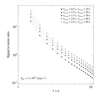
Figure 8: Signal to noise ratio of $140/\left(1+z\right)$–$350/\left(1+z\right)$ keV light curves for simulated pulses. Top panel: $L_{\rm pk}$ = $1\times 10^{50}$ ergs.s^-1, middle panel: $L_{\rm pk}$ = $1\times 10^{51}$ ergs.s^-1, $L_{\rm pk}$ = $1\times 10^{52}$ ergs.s^-1.

Figure 8 demonstrates the two trends seen in Figure 7. First, signal-to-noise ratio reduces with increasing redshift for any given pulse. More importantly, the total signal-to-noise ratio at any given redshift increases with increasing pulse duration. It is important to note, however, that the values of signal-to-noise ratio do not directly compare to those at which the Swift/BAT trigger, due to a varying energy range. Notably, at high redshifts, the width of the light curve energy band decreases significantly as it is defined in the rest frame of the GRB.

An underlying feature of the observed sample of GRBs available in this work is that they must initially be detected by Swift/BAT. This means that, despite using a rest frame defined energy band to mitigate the energy dependence within the measured durations, the sample is fundamentally defined in the observer frame by the triggering criteria of Swift/BAT.

Despite Swift/BAT having a plethora of trigger criteria, the majority of Swift/BAT triggered GRBs are the result of “rate triggers”, which respond to a rapid increase in flux as quantified by a signal-to-noise ratio. As shown in Figure 8, such a signal to noise ratio threshold effectively corresponds to a threshold in duration for a burst with a given observed brightness.

If we consider that the Swift/BAT is intrinsically limited in the durations that can be detected in the observer frame, such that only bursts with $T_{\rm 90,obs}\left(15-35{\rm keV}\right)>T_{\rm 90,critical}\left(15-35{\rm keV}\right)$ result in triggered events, we can show how this would translate into a limit in the duration measured in a rest frame defined energy band.

As $T_{\rm 90,obs}\propto E_{\rm obs}^{-0.4}$ (Norris et al., 1996), we can convert $T_{\rm 90,critical}$ to a duration threshold in a rest frame defined energy band, $T_{\rm 90,critical}^{\prime}$:

$$T_{\rm 90,critical}^{\prime}=T_{\rm 90,critical}\left(\frac{E^{\prime}}{E_{\rm obs}}\right)^{-0.4},$$ (1)

where $E^{\prime}$ and $E_{\rm obs}$ are characteristic energies of the rest frame defined and observer frame defined energy bands, respectively. In Equation 1, both energies have to be in a common frame of reference, and so in the observer frame $E^{\prime}=E_{\rm rest}/\left(1+z\right)$. $E_{\rm rest}$ is the standard characteristic energy of the rest frame defined energy channel, in the rest frame of the GRB. Substituting this definition into Equation 1 yields:

$$T_{\rm 90,critical}^{\prime}=T_{\rm 90,critical}\left(\frac{E_{\rm rest}}{\left(1+z\right)E_{\rm obs}}\right)^{-0.4}.$$ (2)

In Equation 2 three quantities are constant: $T_{\rm 90,critical}$, $E_{\rm rest}$ and $E_{\rm obs}$, thus it follows that $T_{\rm 90,critical}^{\prime}\propto\left(1+z\right)^{0.4}$. Given a minimum value of duration defined in an observer frame energy band, that can result in a detectable burst, there is a related limit in a rest frame defined energy band. As shown in Equation 2, this value increases with increasing redshift of the GRB as the conversion between the observer frame defined energy band and rest frame defined energy band becomes large. Thus such an effect censors the data, preventing the measurement of high redshift, shorter duration GRBs. By censoring the parameter space in this way, an artificial signal of a trend is introduced, such that it might appear that $T_{\rm 90,obs}\left(E_{\rm 1,rest}/\left(1+z\right)-E_{\rm 2,rest}/\left(1+z\right)\right)\propto\left(1+z\right)^{0.4}$.

The significance of any trend of increasing duration with increasing redshift above the null value of $\left(1+z\right)^{0.4}$ can be estimated using Equation 3, where $I$ is the fitted index, with a reported uncertainty of $\Delta I$ and $I_{0}=0.4$ is the null value expected as a result of censorship:

$$\sigma=\frac{|I-I_{0}|}{\Delta I}.$$ (3)

Applying Equation 3 to the fitted indices reported in Table 3 we find that 4 of the 6 relations have significances less than one sigma. When considering the geometric average of $T_{\rm 50,obs}\left(1+z\right)$ for the full sample, the putative correlation has a significance of 1.8$\sigma$, while that of the full sample for $T_{\rm R45,obs}$ has a significance of 3.4$\sigma$. In all cases, this significance reduces when applying the brightness threshold used by Zhang et al. (2013). This is because such a threshold increases the level of censorship of the data. The indices in all cases move to values compatible with $I_{0}=0.4$.

4.3 Sampling the brightest GRBs

We also considered only the brightest GRBs in the full sample. Unlike Zhang et al. (2013), we considered the average signal-to-noise ratio as defined in § 4.2 as this is a better indicator of the total brightness of the prompt emission, whereas $F_{\rm pk}$ is biased towards only the brightest region of a light curve.

We took all bursts with a signal-to-noise ratio above the median value and a measurable value for all three durations considered in this work. We binned the data according to redshift and performed a fit to the geometric average of each duration measure as before. The durations as functions of redshift are plotted in Figure 9.

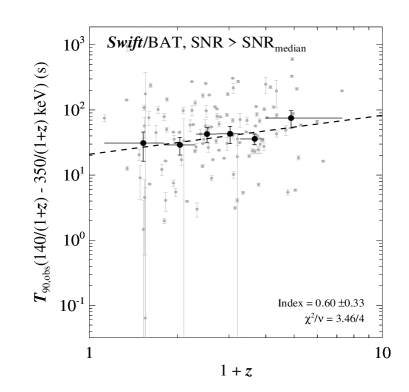
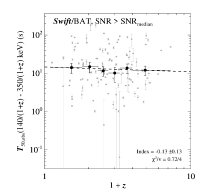
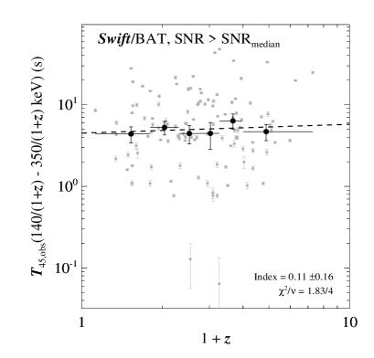
Figure 9: $T_{\rm 90,obs}$, $T_{\rm 50,obs}$ and $T_{\rm R45,obs}$ obtained in the $140/\left(1+z\right)$–$350/\left(1+z\right)$ keV energy range for 116 highest signal-to-noise ratio GRBs in the full Swift/BAT. Grey points correspond to the individual GRBs, while black points are the geometric average. Binning of GRBs is identical in all three panels. The black dashed line in each panel corresponds to a power-law fitted to the average bins. The $\chi^{2}$ fit statistics, degrees of freedom and power-law indices of all three models are indicated in each panel.

Table 6: Details of fits to geometric average of duration as a function of $\left(1+z\right)$ for the bright GRB sample. $N_{\rm GRBs}$ are the number of bursts contained in all six bins, while $\log_{10}N$ is the logarithm of the normalisation to each fitted power-law.

Duration	$N_{\rm GRBs}$	$\log_{10}N$	Index	$\chi^{2}/\nu$
$T_{\rm 90,obs}$	116	1.32 $\pm$0.17	0.60 $\pm$0.33	3.46/4
$T_{\rm 50,obs}$	116	1.17 $\pm$0.06	-0.13 $\pm$0.13	0.72/4
$T_{\rm RT45,obs}$	116	0.65 $\pm$0.07	0.11 $\pm$0.16	1.83/4

As shown in Table 6, the evolution of $T_{\rm 90,obs}\left({\rm SNR}>{\rm SNR}_{\rm median}\right)$ reproduces a very similar best fit model to the bright sample as defined by $F_{\rm pk}$ outlined in § 3.2. The power-law index retrieved from fitting the geometric average to $T_{\rm 90,obs}\left({\rm SNR}>{\rm SNR}_{\rm median}\right)$ is 0.60 $\pm$0.33, giving a significance of only 0.6$\sigma$ to the trend.

However, the fits obtained for $T_{\rm 50,obs}\left({\rm SNR}>{\rm SNR}_{\rm median}\right)$ and $T_{\rm R45,obs}\left({\rm SNR}>{\rm SNR}_{\rm median}\right)$ are consistent, within error, with being constant with redshift, which would imply that $T_{\rm 50,rest}$ and $T_{\rm R45,rest}$ in the brightest half of Swift/BAT GRBs reduce with increasing redshift, such that $T_{\rm 50,rest}\left({\rm SNR}>{\rm SNR}_{\rm median}\right)\propto\left(1+z\right)^{-1}$. Considering the errors in the fitted indices, which are of the same order of magnitude as the indices themselves (-0.13 $\pm$0.13 for $T_{\rm 50,obs}$, and 0.11 $\pm$0.16 for $T_{\rm R45,obs}$), this is not likely a physical effect, as it suggests correlations strengths of $\lesssim$1$\sigma$.

5 Conclusions

In this work we have investigated whether duration measures of Swift/BAT and Fermi/GBM detected GRBs exhibit the effects of cosmological time dilation. We first verify the results of Zhang et al. (2013) and investigate which method of averaging individual durations is the most robust as shown in Figure 2. As a power-law model is employed, we choose the geometric average.

We find that, when accounting for the measured errors in $T_{\rm 90,obs}$, a power-law is a statistically unacceptable fit to individual bright GRBs as shown in Figure 3. We then updated the Swift/BAT sample to include an additional 93 GRBs that have occurred since the original analysis by Zhang et al. (2013). Using this total sample of 232 bursts we investigate the evolution of average durations $T_{\rm 90,obs}$, $T_{\rm 50,obs}$ and $T_{\rm R45,obs}$ as a function of redshift in the $140/\left(1+z\right)$–$350/\left(1+z\right)$ keV range. All three durations exhibit a trend of increasing with increasing redshift. The power-law indices of these trends were reduced when filtering out bursts with poorly measured values of duration.

The model power-law index obtained fitting the geometric average of $T_{\rm 50,obs}\left(140/\left(1+z\right)-350/\left(1+z\right)~{}{\rm keV}\right)$ has a value most consistent with that expected from time-dilation. We do find, however, that the large scatter of the distribution of individual duration values is large, leading to large statistical errors on each average bin, and therefore a large error in the fitted parameters of the power-law model.

We also compare the distributions of all three durations, in the rest frame, both above and below the median redshift $z_{\rm median}$, and within the upper and lower quartiles of redshift. Using the Student’s $t$-test we find that the distributions of durations are consistent with having the same mean value in five out of six cases. We also find a 3$\sigma$ difference in $T_{\rm R45,obs}\left(140/\left(1+z\right)-350/\left(1+z\right)~{}{\rm keV}\right)/\left(1+z\right)$ distributions above and below $z_{\rm median}$. Of the three duration measures, it is perhaps expected that $T_{\rm R45,obs}$ would show the least evidence of cosmological time dilation. $T_{\rm R45,obs}$ contains only the brightest regions of a light curve. Conversely, should any quiescent period be present between prompt pulses, $T_{\rm 90,obs}$ and $T_{\rm 50,obs}$ will contain this time. Kocevski & Petrosian (2013) propose that such quiescent periods between pulses are likely to be the best tracers of cosmological time dilation.

We cross-referenced the 232 Swift/BAT GRBs with Fermi/GBM data, to find that 57 bursts with redshift have been detected with both instruments. Figure 6 demonstrates that this sample is dominated by small number statistics. As such the Swift/BAT data in this subset of bursts does not reflect the trends shown for the full sample. For all three duration measures, the obtained Fermi/GBM seem to evolve more weakly with redshift than those obtained for the same GRBs with the Swift/BAT. The significance of this difference is not high, however, once more due to the small size of the joint sample.

We finally consider the origin of the apparent durations trends as a function of redshift, to assess whether the physical origins are due to the cosmological time dilation of a common rest frame distribution of GRBs. We find no evidence of under-sampling of the long duration, low redshift region of the parameter space.

We then demonstrate the dearth of high-redshift, short duration (where short refers to the low duration end of the long GRB distribution) can be attributed to censorship of the parameter space. This censorship arises from originally creating the sample of detected GRBs in an observer frame energy band, as this is how Swift/BAT triggers are defined. As BAT triggers have a signal-to-noise ratio threshold and, for a given peak flux, shorter GRBs have lower significance, this naturally places a minimum limit of detectable duration for a long GRB of a given brightness. This limit can be converted to an equivalent limit in the duration distribution of the rest frame defined energy band. As the difference between the observer frame defined and rest frame defined energy bands increases with increasing redshift, the lower limit in detectable durations rises accordingly. Thus the high redshift, low duration region of the parameter space suffers from censorship, which helps to artificially induce a signature of cosmological time dilation in the duration-redshift plane. This censorship increases as $\left(1+z\right)^{0.4}$, thus giving a null hypothesis value for the power-law index of any duration-redshift relation. Assessing the significance of the relations found in this work, we find that they typically are less than 1 or 2$\sigma$.

Finally, we isolate bursts that are well detected by the Swift/BAT instrument. Our metric for “brightness” is also an average signal-to-noise ratio over the entire burst duration, thus ensuring the pulse tail is well sampled. In so doing, we find that the geometric average of $T_{\rm 90,obs}$ may still correlate with redshift, although $T_{\rm 50,obs}$ and $T_{\rm R45,obs}$ do not appear to. The reason for the difference between the three measures may result from $T_{\rm 90}$ being defined in such a way that it is more likely to include any quiescent periods between pulses in the prompt light curve. These will very strongly exhibit the effects of cosmological time-dilation. Care must be taken when imposing such thresholds, however, as they potentially enhance the censorship effects previously discussed, by strengthening the thresholds in signal-to-noise ratio any GRB must satisfy to be considered in the sample.

This work highlights the relative merits of each of the three duration measures. Of the three, $T_{\rm 90}$ comes the closest to capturing the total prompt duration. However, in doing so, it is necessary to deeply probe the tail of pulse emission. The uncertainty, therefore in determining the end of the $T_{\rm 90}$ duration can be high. $T_{\rm R45}$ only captures a sense of the brightest regions of a burst. Initially, this seems a promising prospect for extracting cosmological time dilation if one assumes pulses to be self-similar in the rest frame. However, the population of pulses within prompt light curves is diverse (Norris et al., 2005). Additionally, $T_{\rm R45}$ does not contain information concerning the frequency of bright emission periods. That is to say, without further information, it is not known if $T_{\rm R45}$ is continuous, or comprised of several shorter episodes.

$T_{\rm 50}$ could be considered to offer more information than both $T_{\rm 90}$ and $T_{\rm R45}$ can individually. By considering a narrower region of the cumulative distribution of prompt emission, $T_{\rm 50}$ samples the pulse tail to a point that is better defined in signal-to-noise ratio. However, $T_{\rm 50}$ still provides a better estimate of total prompt duration when compared to $T_{\rm R45}$ as it can include intervening quiescent periods between bright pulses.

Given the scatter of the distributions of durations, and the unavoidable censorship of the redshift-duration parameter space, the quest for a redshift or luminosity indicator within high-energy prompt GRB light curves seems unlikely to yield a positive result.

References

- Ajello et al. (2008) Ajello M., Greiner J., Sato G., Willis D. R., Kanbach G., Strong A. W., Diehl R., Hasinger G., Gehrels N., Markwardt C. B., Tueller J., 2008, ApJ, 689, 666
- Barthelmy et al. (2005) Barthelmy S. D., et al., 2005, Space Sci. Rev., 120, 143
- Burrows et al. (2005) Burrows D. N., et al., 2005, Space Sci. Rev., 120, 165
- Butler et al. (2010) Butler N. R., Bloom J. S., Poznanski D., 2010, ApJ, 711, 495
- Butler et al. (2007) Butler N. R., Kocevski D., Bloom J. S., Curtis J. L., 2007, ApJ, 671, 656
- Cao et al. (2011) Cao X.-F., Yu Y.-W., Cheng K. S., Zheng X.-P., 2011, MNRAS, 416, 2174
- Frontera et al. (2009) Frontera F., Guidorzi C., Montanari E., Rossi F., Costa E., Feroci M., Calura F., Rapisarda M., Amati L., Carturan D., Cinti M. R., Fiume D. D., Nicastro L., Orlandini M., 2009, ApJS, 180, 192
- Gehrels et al. (2004) Gehrels N., et al., 2004, ApJ, 611, 1005
- Gruber et al. (1999) Gruber D. E., Matteson J. L., Peterson L. E., Jung G. V., 1999, ApJ, 520, 124
- Hjorth et al. (2012) Hjorth J., Malesani D., Jakobsson P., Jaunsen A. O., Fynbo J. P. U., Gorosabel J., Krühler T., Levan A. J., Michałowski M. J., Milvang-Jensen B., Møller P., Schulze S., Tanvir N. R., Watson D., 2012, ApJ, 756, 187
- Kaneko et al. (2006) Kaneko Y., Preece R. D., Briggs M. S., Paciesas W. S., Meegan C. A., Band D. L., 2006, ApJS, 166, 298
- Klebesadel et al. (1973) Klebesadel R. W., Strong I. B., Olson R. A., 1973, ApJ, 182, L85
- Kocevski & Petrosian (2013) Kocevski D., Petrosian V., 2013, ApJ, 765, 116
- Kolaczyk (1997) Kolaczyk E. D., 1997, ApJ, 483, 340
- Kouveliotou et al. (1993) Kouveliotou C., Meegan C. A., Fishman G. J., Bhat N. P., Briggs M. S., Koshut T. M., Paciesas W. S., Pendleton G. N., 1993, ApJ, 413, L101
- Littlejohns et al. (2013) Littlejohns O. M., Tanvir N. R., Willingale R., Evans P. A., O’Brien P. T., Levan A. J., 2013, MNRAS, 436, 3640
- Lupton (1993) Lupton R., 1993, Statistics in theory and practice
- Margutti et al. (2010) Margutti R., Guidorzi C., Chincarini G., Bernardini M. G., Genet F., Mao J., Pasotti F., 2010, MNRAS, 406, 2149
- Meegan et al. (2009) Meegan C., et al., 2009, ApJ, 702, 791
- Metzger et al. (1997) Metzger M. R., Djorgovski S. G., Kulkarni S. R., Steidel C. C., Adelberger K. L., Frail D. A., Costa E., Frontera F., 1997, Nature, 387, 878
- Nakar (2007) Nakar E., 2007, Phys. Rep., 442, 166
- Norris (2002) Norris J. P., 2002, ApJ, 579, 386
- Norris et al. (2005) Norris J. P., Bonnell J. T., Kazanas D., Scargle J. D., Hakkila J., Giblin T. W., 2005, ApJ, 627, 324
- Norris et al. (2000) Norris J. P., Marani G. F., Bonnell J. T., 2000, ApJ, 534, 248
- Norris et al. (1996) Norris J. P., Nemiroff R. J., Bonnell J. T., Scargle J. D., Kouveliotou C., Paciesas W. S., Meegan C. A., Fishman G. J., 1996, ApJ, 459, 393
- Quilligan et al. (2002) Quilligan F., McBreen B., Hanlon L., McBreen S., Hurley K. J., Watson D., 2002, A&A, 385, 377
- Reichart et al. (2001) Reichart D. E., Lamb D. Q., Fenimore E. E., Ramirez-Ruiz E., Cline T. L., Hurley K., 2001, ApJ, 552, 57
- Sakamoto et al. (2011) Sakamoto T., Barthelmy S. D., Baumgartner W. H., Cummings J. R., Fenimore E. E., Gehrels N., Krimm H. A., Markwardt C. B., Palmer D. M., Parsons A. M., Sato G., Stamatikos M., Tueller J., Ukwatta T. N., Zhang B., 2011, ApJS, 195, 2
- Salvaterra et al. (2012) Salvaterra R., et al., 2012, ApJ, 749, 68
- Ukwatta et al. (2012) Ukwatta T. N., Dhuga K. S., Stamatikos M., Dermer C. D., Sakamoto T., Sonbas E., Parke W. C., Maximon L. C., Linnemann J. T., Bhat P. N., Eskandarian A., Gehrels N., Abeysekara A. U., Tollefson K., Norris J. P., 2012, MNRAS, 419, 614
- von Kienlin et al. (2014) von Kienlin A., et al., 2014, ApJS, 211, 13
- Zhang et al. (2013) Zhang F.-W., Fan Y.-Z., Shao L., Wei D.-M., 2013, ApJ, 778, L11