Negative modes of Coleman-De Luccia bounces

Abstract

We investigate the negative modes about Coleman-De Luccia bounces governing vacuum transitions in de Sitter space, with the goal of gaining physical insight into the various anomalous results associated with these that have been reported in the literature. For the case of bounces with radii much less that the horizon distance $H^{-1}$ we find two distinct regimes, distinguished by the magnitude of the bubble nucleation rate $\Gamma$. If $\Gamma/H^{4}\gg 1$, then the behavior of the modes contributing to the determinant factors in $\Gamma$ is much as it is in flat spacetime, and the calculation of $\Gamma$ goes over smoothly to the flat spacetime calculation as the gravitational coupling is taken to zero. This is not the case if $\Gamma/H^{4}\ll 1$. These two regimes correspond to the two possible outcomes of de Sitter vacuum decay — either a rapidly completed transition or non-percolation and eternal inflation. For bounces with radii comparable to the horizon length, we confirm previous results concerning anomalous negative modes with support on the bounce wall. We also find further evidence supporting previous claims, based on thin-wall arguments, of the absence of expected negative modes for a class of bounces that arises when the initial and final vacua are nearly degenerate.

I Introduction

The process in which a false vacuum of a scalar field theory decays by the nucleation of true vacuum bubbles was first studied in detail some time ago Kobzarev:1974cp ; Coleman:1977py . The bubble nucleation rate has the exponential suppression typical of tunneling processes, with the exponent being twice the WKB barrier penetration integral or, equivalently, the Euclidean action of the bounce solution to the Euclidean field equations Coleman:1977py . By using path integral methods to calculate the energy density of the false vacuum, the pre-exponential factor can also be obtained Callan:1977pt . This turns out to contain a factor of $[\det S_{E}^{\prime\prime}(\phi_{\rm bounce})]^{-1/2}$, where $S_{E}^{\prime\prime}$ denotes the second functional variation of the Euclidean action. An essential ingredient of this calculation is the fact that $S_{E}^{\prime\prime}(\phi_{\rm bounce})$ has a single negative eigenvalue, which arises from a mode corresponding to expansion or contraction of the bounce. Because of the square root, this negative mode leads to a factor of $i$ that makes the false vacuum energy complex, with its imaginary part interpreted in terms of a rate of decay by bubble nucleation. It is crucial here that there is only a single negative eigenvalue and thus one factor of $i$; if, for example, there were an even number of such eigenvalues, the contribution to the false vacuum energy would be purely real. Indeed, it has been shown that the bounce with lowest action has one, and only one, negative mode Coleman:1987rm .

Coleman and De Luccia (CDL) Coleman:1980aw proposed that this formalism could be extended to include gravitational effects by adding a Euclidean Einstein-Hilbert term to the action. Although they did not address the issue of the prefactor, it seems natural to assume that it should be analogous to that for the non-gravitational case, and that the dominant bounce should again have a single negative mode. The matter is complicated by the fact that with gravity included the fluctuations about the bounce enjoy a gauge freedom, corresponding to the invariance under coordinate transformations of the underlying theory. A consequence of this gauge freedom is the existence of constraints that must be imposed on the possible fluctuations.

A number of authors have studied the negative mode issue in the context of bounces corresponding to bubble nucleation in a de Sitter spacetime Lavrelashvili:1985vn ; Tanaka:1992zw ; Garriga:1993fh ; Tanaka:1999pj ; Gratton:1999ya ; Khvedelidze:2000cp ; Lavrelashvili:1999sr ; Gratton:2000fj ; Dunne:2006bt . Some curious, troubling, and sometimes contradictory, results, often depending on the choice of gauge, have been obtained. Among these are:

1) An action for fluctuations about a bounce with large radius that is unbounded from below, suggesting an infinite family of negative modes with support near the bubble wall.

2) Indications of a similar phenomenon for all de Sitter CDL bounces, but with the additional negative modes having support on a region defined by the horizon.

3) Arguments for the existence of a single negative mode, but subject to restrictions on the form of the bounce solution.

4) Claims that there are no negative modes, and that the factor of $i$ comes from a proper rotation of contours in the Hamiltonian path integral.

5) The absence of a negative mode in the thin-wall approximation for a certain class of bounces.

In our view, these works only address one part of the problem, namely how to develop an algorithm that, at least in principle, gives an unambiguous result for the bubble nucleation rate. There is another aspect that should be addressed. When anomalous or apparently meaningless mathematical results are encountered, it is often the case that they are indicative of a particular physical aspect of the problem being studied. Thus, one should look for a physical understanding as to why these negative modes arise (or do not) in particular cases, even if they can ultimately be eliminated from the calculation. Also, one should expect to find a smooth transition from the curved spacetime calculation to the non-gravitational one in an appropriate limit. Ideally, this should include not just a continuous evolution of the bounce and its action, but also a gradual disappearance of the potential pathologies as one approaches the limit in which $\kappa\equiv 8\pi G=0$. As we will see, this limit is rather subtle.

Our goal in this paper is to make some progress toward this end by exploring the regions where the quadratic fluctuation action becomes negative. We work in a purely Lagrangian framework. Rather than fixing a gauge, we impose the requirement that the fluctuations obey the constraint, and then write the quadratic fluctuation Lagrangian in terms of manifestly gauge-invariant combinations of fields. For fluctuations about a bounce with O(4)-symmetry, which we assume, the objects of primary interest are spherically symmetric scalar fluctuations, which can be described by a single field $\chi$. We examine the situations in which $\chi$ can have negative modes, and study the form of those modes as $\kappa$ is varied.

The remainder of this paper is organized as follows. In Sec. II we review the formalism for treating vacuum decay in both flat spacetime (i.e., with gravity ignored) and with gravitational effects included. In Sec. III we discuss negative modes in flat spacetime. In the course of this discussion we describe an example where bounces with many negative modes turn out to not only be physically meaningful, but to actually be dominant. Section IV describes the perturbative expansion of the scalar field and metric about an O(4)-symmetric CDL bounce and gives the expression for the quadratic part of the fluctuation Lagrangian. Next, in Sec. V, we explore the various types of negative modes that can arise from this Lagrangian. Many of the results that we present here are based on numerical explorations of particular scalar field models. In Sec. VI we discuss the negative mode problem for multibounce solutions. This is almost a trivial aside in flat spacetime, but becomes more complex with gravity included. In fact, we will see that it is key to understanding the limit in which gravitational effects disappear. Finally, in Sec. VII we summarize our results and discuss how they reflect the various modes of vacuum decay in de Sitter spacetime. There are two appendices containing some technical details.

II Review of tunneling

II.1 Tunneling in flat spacetime

The WKB approximation leads to an expression of the form

$$\gamma=C\,e^{-B}$$ (1)

for the decay rate of a state that decays by tunneling through a potential energy barrier. For the case of a single particle in one dimension with a standard kinetic energy,

$$B=2\int_{x_{1}}^{x_{2}}dx\,\sqrt{2m[V(x)-E]}\,,$$ (2)

where $x_{1}$ and $x_{2}$ are the classical turning points that bound the particle’s path through the barrier.

With multiple degrees of freedom, the WKB approximation requires that we consider all paths through the barrier and pick out the one along which the one-dimensional tunneling exponent is a minimum Banks:1973ps ; Banks:1974ij . This minimization problem is equivalent to the problem of finding a stationary point of the Euclidean action, which in turn is equivalent to finding a solution of the Euclidean equations of motion Coleman:1977py . The solution relevant for tunneling, known as the bounce, starts at an initial configuration at Euclidean time $\tau_{\rm in}$, runs through the barrier to an exit point at some $\tau_{0}$, and then returns, in a “$\tau$-reversed” fashion, to $\tau_{\rm fin}$. The intermediate Euclidean times give a parameterization of the tunneling path through configuration space. If the initial configuration is a local minimum of the potential energy (i.e., a false vacuum), then $\tau_{\rm in}=-\infty$ and $\tau_{\rm fin}=\infty$.

For a scalar field theory with a standard Lagrangian the tunneling exponent $B$ is equal to the difference between the Euclidean actions of the bounce solution $\phi(x)$ and the uniform false vacuum. Even if these actions are divergent, their difference,

$$B = S_{E}(\phi)-S_{E}(\phi_{\rm fv})$$ (3)

$$= \int_{-\infty}^{\infty}d\tau\int d^{3}x\,\left[\frac{1}{2}\left({d\phi\over d\tau}\right)^{2}+\frac{1}{2}({\bm{\nabla}}\phi)^{2}+U(\phi)-U(\phi_{\rm fv})\right]\,,$$ (4)

is finite and well-defined. Note that the tunneling integral and the Euclidean action differ for paths that are not solutions of the equations of motion. In fact, although the bounce is a local minimum of the integral through the potential energy barrier, it only corresponds to a saddle point of $S_{E}$.

In a scalar field theory, with thermal and gravitational effects ignored, the bounce describing tunneling from a false vacuum is a solution on Euclidean $R^{4}$ that approaches the false vacuum value $\phi_{\rm fv}$ as either $|{\bf x}|$ or $\tau$ tends to infinity. With only minimal restrictions on the potential $U(\phi)$, it can be shown that the bounce with the smallest action is O(4)-symmetric Coleman:1977th . Figure 1 illustrates such a bounce.

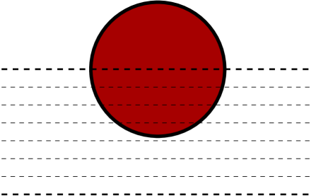
Figure 1: Schematic view of a bounce in flat spacetime. The shaded region represents the region of approximate true vacuum. This is separated from the false vacuum exterior by the wall region represented by the solid black line. (In actuality the field has an exponential tail and only reaches its exact false vacuum value at $\tau=-\infty$.) The horizontal dashed lines represent hypersurfaces of constant $\tau$ that trace out a path in configuration space. The heavy dashed lines correspond to the initial pure vacuum configuration and to the final field configuration at bubble nucleation.

The prefactor $C$ can be obtained by a path integral argument Callan:1977pt . Consider the matrix element

$$\langle\phi_{\rm fv}|e^{-HT}|\phi_{\rm fv}\rangle = \int[d\phi({\bf x},\tau)]\,e^{-S_{E}[\phi]}$$ (5)

$$= \sum_{n}e^{-E_{n}T}\langle\phi_{\rm fv}|n\rangle\langle n|\phi_{\rm fv}\rangle\,.$$ (6)

Here the path integral is restricted to paths that begin and end on the false vacuum configuration. In the limit $T\to\infty$, the sum over energy eigenstates in the second expression is dominated by the state with the lowest energy among those that contribute to the matrix element. Identifying this state as the false vacuum, we have

$$E_{\rm fv}=-\lim_{T\to\infty}{1\over T}\ln\,\langle\phi_{\rm fv}|e^{-HT}|\phi_{\rm fv}\rangle\,.$$ (7)

The path integral is evaluated by expanding about its stationary points. The first of these is the constant solution with $\phi(x)=\phi_{\rm fv}$ everywhere. A Gaussian integral about this gives

$$I_{0}=[\det S_{E}^{\prime\prime}(\phi_{\rm fv})]^{-1/2}\,e^{-S_{E}(\phi_{\rm fv})}\,,$$ (8)

where $S^{\prime\prime}_{E}$ denotes the second functional derivative of the Euclidean action. It is convenient to consider space to have a finite volume $\Omega$ which is to be taken to infinity at the end of the calculation, so that $S_{E}(\phi_{\rm fv})=\Omega T\,U(\phi_{\rm fv})$.

Next, we have the bounce solution. This would give a similar Gaussian integral were it not for two factors. First, the spectrum of $S^{\prime\prime}_{E}(\phi_{\rm bounce})$ includes four zero modes, corresponding to the freedom to translate the bounce in Euclidean space and time. These are handled by introducing collective coordinates specifying the location of the center of the bounce. Second, the spectrum also contains a mode with negative eigenvalue, corresponding roughly (and exactly, in the thin-wall limit) to expansion or contraction of the bounce. This negative mode leads to a factor of $i$ when the square root of the determinant is taken. The contribution to the path integral can be written as

$$I_{1} = \frac{i}{2}\,\Omega T\left|{\det^{\prime}S_{E}^{\prime\prime}(\phi_{\rm bounce})]\over\det S_{E}^{\prime\prime}(\phi_{\rm fv})}\right|^{-1/2}\,J\,e^{-[S_{E}(\phi_{\rm bounce})-S_{E}(\phi_{\rm fv})]}\,I_{0}$$ (9)

$$\equiv i\Omega TKe^{-B}\,I_{0}\,.$$ (10)

Here the factor of $\Omega T$ arises from integrating over the four collective coordinates, $J$ contains the Jacobian factors associated with the introduction of the collective coordinates, and the factor of 1/2 comes from a careful treatment of the negative mode. Finally, the prime on the bounce determinant indicates that the product of eigenvalues is to be taken only over the nonzero eigenvalues.

There are also approximate stationary points corresponding to many well-separated bounces. The $n$-bounce solution has an action

$$S_{E}(\phi_{n\rm-bounce})=S_{E}(\phi_{\rm fv})+n\left[S_{E}(\phi_{\rm bounce})-S_{E}(\phi_{\rm fv})\right]=S_{E}(\phi_{\rm fv})+nB\,.$$ (11)

The integration over the collective coordinates gives a factor of $(\Omega T)^{n}/n!$, with the $n!$ entering because the bounces are indistinguishable. Similarly, the factor of $J$ becomes $J^{n}$. Only the determinant factors remain to be considered.

Outside the wall region the bounce solution rapidly approaches the pure false vacuum, with $|\phi_{\rm bounce}(x)-\phi_{\rm fv}|$ decreasing exponentially with distance. Thus, we can imagine evaluating the determinant for the one-bounce case by dividing Euclidean space into a large (compared to the bounce radius) region enclosing the bounce, and the remainder. The full determinant is then the product of the contributions of the two regions. In the latter region the bounce is exponentially close to the false vacuum and the contributions to the bounce and the false vacuum determinants are essentially equal. In the region containing the bounce the determinants corresponding to $\phi_{\rm bounce}$ and $\phi_{\rm fv}$ differ precisely by the ratio that appears in Eq. (10).

For an $n$-bounce configuration, with the bounces all well separated, the Euclidean spacetime can be divided into $n$ regions, each containing one bounce, and the remainder, in which the field is essentially equal to its false vacuum region. The full determinant is the product of the contributions from each of these regions. The net result is that the contribution to the path integral from $n$-bounce configurations is

$$I_{n}={1\over n!}\left(i\Omega TKe^{-B}\right)^{n}I_{0}\,.$$ (12)

Summing the contributions from all values of $n$ gives

$$I = I_{0}\sum_{n=0}^{\infty}{1\over n!}\left(i\Omega TKe^{-B}\right)^{n}$$ (13)

$$= I_{0}\exp\left[i\Omega TKe^{-B}\right]\,.$$ (14)

Taking the logarithm and using Eq. (7) gives

$$E_{\rm fv}=-\lim_{T\to\infty}\left({\ln\,I_{0}\over T}\right)-i\Omega Ke^{-B}\,.$$ (15)

The first term on the right-hand side is real, but the second is imaginary, making the false vacuum energy complex. As usual, we interpret this as a signal that the false vacuum is unstable, with a decay rate

$$\gamma=-2\,{\rm Im}\,E_{\rm fv}=2\Omega Ke^{-B}\,.$$ (16)

This is proportional to $\Omega$, corresponding to the fact that a bubble can nucleate anywhere in space. The bubble nucleation rate per unit volume is

$$\Gamma=2K\,e^{-B}\,.$$ (17)

This calculation implicitly assumes that in the multibounce solutions the individual bounces are separated by distances large relative to the bounce four-volume ${\cal V}_{b}$. To test this dilute-gas approximation, we note that the sum in Eq. (14) is dominated by the terms with

$$n\approx\Omega TKe^{-B}\,.$$ (18)

For the approximation to be valid, we must require that the volume occupied by these $n$ bounces be much less than the total Euclidean spacetime volume $\Omega T$; i.e.,

$${\cal V}_{4}Ke^{-B}\ll 1\,,$$ (19)

where ${\cal V}_{4}$ is the four-dimensional volume of the bounce. Dimensional arguments suggest that ${\cal V}_{4}K$ is typically of order unity, in which case this condition reduces to a lower bound on $B$.

A useful illustrative example is given by the thin-wall approximation, which applies in the limit where the difference between the false and true vacuum values of the potential, $\epsilon\equiv U(\phi_{\rm fv})-U(\phi_{\rm tv})$, is sufficiently small relative to the surface tension $\sigma$ of the bubble Coleman:1977py . The bounce can then be obtained by considering O(4)-symmetric configurations in which a true vacuum region of radius $R$ is separated from the exterior false vacuum by a thin wall with action per unit area $\sigma$. The total Euclidean action, less that of the pure false vacuum, is

$$S_{E}(R)=2\pi^{2}\sigma R^{3}-{\pi^{2}\over 2}\,\epsilon R^{4}\,.$$ (20)

The stationary point of this action at $\bar{R}\equiv 3\sigma/\epsilon$ gives the bounce radius. Both the bounce radius and the tunneling exponent

$$B={27\pi^{2}\over 2}\,{\sigma^{4}\over\epsilon^{3}}$$ (21)

tend to infinity in the $\epsilon\to 0$ limit of degenerate vacua. The fact that

$$\left.{d^{2}S_{E}\over dR^{2}}\right|_{\bar{R}}=-{18\pi^{2}\sigma^{2}\over\epsilon}$$ (22)

is negative shows that the bounce is a maximum of the action among the one-parameter family of thin-wall configurations, and thus a saddle point of the action, with at least one negative eigenvalue, on the full configuration space.

Finally, recall that the bounce is supposed to describe a family of configurations interpolating between the initial pure vacuum state, at $\tau=-\infty$, and a state of equal potential energy containing a bubble, on a constant $\tau$ slice through the center of the bounce. In the thin-wall limit the difference in the static potential energy between these two configurations is

$$\Delta E=4\pi R^{2}\sigma-\frac{4}{3}\pi R^{3}\epsilon\,.$$ (23)

This does indeed vanish if $R=\bar{R}$.

The above discussion readily generalizes to the case of nonzero temperature $T$ Linde:1981zj . In this case $\Gamma$ is obtained from the imaginary part of the free energy, rather than the energy, of the metastable false vacuum. The Euclidean path integral is then over paths that are periodic in Euclidean time with period $\beta=1/T$. Furthermore, the classical Euclidean equations leading to the bounce must be obtained using the finite-temperature effective potential. Just as at $T=0$, the path integral includes contributions not just from a single bounce, but also from all multibounce solutions. Summing over these exponentiates the single bounce contribution, and the nucleation rate can be read off from the exponent.

II.2 Including gravitational effects

Coleman and De Luccia Coleman:1980aw argued that gravitational effects could be incorporated by adding a Euclidean Einstein-Hilbert term to the action, so that

$$S_{E}=\int d^{4}x\sqrt{g}\left[-{1\over 2\kappa}R+\frac{1}{2}\,g^{ab}\partial_{a}\phi\,\partial_{b}\phi+U(\phi)\right]+S_{\rm bdy}\,,$$ (24)

where $\kappa=8\pi G$ and $S_{\rm bdy}$ is the Euclidean version of the Gibbons-Hawking boundary term Gibbons:1976ue .

Although it has not been proven that the bounce of minimum action continues to be O(4)-symmetric when gravitational effects are included, this is widely believed to be true. If one assumes this to be the case, the Euclidean metric can be written as

$$ds^{2}=N(\xi)d\xi^{2}+\rho(\xi)^{2}d\Omega_{3}^{2}\,,$$ (25)

where $d\Omega_{3}^{2}$ is the usual metric on the unit three-sphere. It is convenient to choose the origin of $\xi$ to be a zero of $\rho$, so that $\rho(0)=0$. The curvature scalar is

$$R={6\over N\rho^{2}}\left(N-{\dot{\rho}}^{2}-\rho\ddot{\rho}\right)+{3\dot{\rho}\dot{N}\over\rho N^{2}}\,,$$ (26)

with overdots denoting derivatives with respect to $\xi$.

With the scalar field $\phi$ depending only on $\xi$, the Euclidean action takes the form

$$S_{E}=2\pi^{2}\int d\xi\sqrt{N}\left\{\rho^{3}\ \left[{1\over 2N}\,{\dot{\phi}}^{2}+U(\phi)\right]+\frac{3}{\kappa}\left[{1\over N}\left(\rho^{2}\ddot{\rho}+\rho{\dot{\rho}}^{2}\right)-\rho-{\rho^{2}\dot{\rho}\dot{N}\over 2N^{2}}\right]\right\}+S_{\rm bdy}\,.$$ (27)

An integration by parts to remove the second derivative term recasts this as

$$S_{E}=2\pi^{2}\int d\xi\sqrt{N}\left\{\rho^{3}\left[{1\over 2N}\,{\dot{\phi}}^{2}+U(\phi)\right]-\frac{3}{\kappa}\left({\rho{\dot{\rho}}^{2}\over N}+\rho\right)\right\}\,,$$ (28)

with the boundary terms from the integration by parts precisely canceling $S_{\rm bdy}$.

We note that the action does not contain any derivatives of $N$. Consequently, variation with respect to $N$ yields a constraint equation (which is in fact the $G_{\xi\xi}$ Einstein equation),

$$0=\rho^{3}\left({{\dot{\phi}}^{2}\over 2N}-U\right)-{3\over\kappa}\left({\rho{\dot{\rho}}^{2}\over N}-\rho\right)\,.$$ (29)

The existence of this constraint is related to the freedom to make a coordinate transformation to redefine $\xi$. We make use of this gauge freedom to set $N(\xi)=1$. Having done so, we can write the constraint equation as

$${\dot{\rho}}^{2}=1+{\kappa\over 3}\,\rho^{2}\left(\frac{1}{2}{\dot{\phi}}^{2}-U\right)\,.$$ (30)

Varying the action with respect to $\phi$ gives the scalar field equation of motion

$$\ddot{\phi}+{3\dot{\rho}\over\rho}\dot{\phi}={dU\over d\phi}\,.$$ (31)

Equations (30) and (31) are a complete set of field equations. Variation of the action with respect to $\rho$ does not yield an independent equation, reflecting the fact that in spherically symmetric configurations the gravitational dynamics is determined completely by the matter distribution. However, differentiating Eq. (30) and then using Eq. (31) yields the useful identity

$$\ddot{\rho}=-\frac{\kappa}{3}\,\rho\left(\dot{\phi}^{2}+U\right)\,.$$ (32)

For bubble nucleation in a Minkowski or anti-de Sitter false vacuum the bounce solution has the topology of $R^{4}$, just as in the non-gravitational case. De Sitter spacetime, the case on which we will focus, is different. In this case $\rho$ always has a second zero, at a value $\xi=\xi_{\rm max}$. The bounce is then topologically a four-sphere, with a finite four-volume of order $H^{-4}$, where

$$H=\sqrt{{\kappa\over 3}\,U(\phi_{\rm fv})}$$ (33)

is the Hubble parameter of the false vacuum. In particular, for the solution of Eqs. (30) and (31) describing the pure false vacuum, with $\phi=\phi_{\rm fv}$ everywhere, the metric is the standard round metric on the four-sphere, with

$$\rho=H^{-1}\sin(H\xi)\,.$$ (34)

Its Euclidean action, which must be subtracted from that of the bounce to obtain $B$, is

$$S_{E}=-{24\pi^{2}\over\kappa^{2}\,U(\phi_{\rm fv})}=-{8\pi^{2}\over\kappa}\,H^{-2}\,.$$ (35)

In our discussions it will be useful to distinguish two classes of bounce solutions:

a) Small bubble bounces: The difference between the values of the potential at the false vacuum and at the top of the barrier defines a mass scale $\mu$ via

$$U_{\rm top}-U_{\rm fv}\equiv\mu^{4}\,.$$ (36)

If $\mu\ll M_{P}$ and the difference between the true and false vacuum values of $U$ is not too small, then the bounce describes the nucleation of bubbles whose radius $\bar{\rho}$ at nucleation is much smaller than $H^{-1}$. If $\xi\ll H^{-1}$, then $\rho(\xi)\approx\xi$ and $\phi(\xi)$ differs only slightly from the corresponding flat-space bounce. For larger $\xi$, on the other hand,

$$\rho=H^{-1}\sin[H(\xi+\Delta)]\,,$$ (37)

where $\Delta=O(\mu/M_{P}^{2})$. The scalar field in this large-$\xi$ region is exponentially close to its false vacuum value, with $|\phi-\phi_{\rm fv}|\sim\mu e^{-\mu(\xi-\bar{\xi})}$.

b) Large bubble bounces: Bubbles of size comparable to $H^{-1}$ can arise, even with $\mu\ll M_{P}$, if $\epsilon$ is sufficiently small. The flat-space thin-wall results are replaced by Parke:1982pm

$${1\over\bar{\rho}^{2}}=H^{2}+\left({\epsilon\over 3\sigma}-{\kappa\sigma\over 4}\right)^{2}\,.$$ (38)

As $\epsilon$ is decreased, the bubble radius increases until it reaches a maximum value, $\bar{\rho}=H^{-1}$, when the quantity in parentheses vanishes. Until this point, the false vacuum region is larger than a hemisphere, while the true vacuum occupies less than a hemisphere. With a further decrease in $\epsilon$, $\bar{\rho}$ begins to decrease, and the true and false vacuum regions are both less than hemispheres. In contrast to the flat-space thin-wall bounce, whose radius and action tend to infinity in the $\epsilon\to 0$ limit, both $\bar{\rho}$ and the bounce action remain finite in this limit. To distinguish between the two regimes, we will denote bounces as being type A or type B, according to whether the false vacuum region is greater than or less than a hemisphere.

We saw in Eq. (22) that with gravity ignored the bounce was a maximum, as a function of $R$, of the thin-wall-approximation action. Similarly, for type A bounces the $\bar{\rho}$ of Eq. (38) gives a maximum of the thin-wall action, and therefore a saddle point of the full action functional Coleman-Steinhardt . However, for type B thin-wall solutions the second derivative of the action with respect to $\bar{\rho}$ is positive, corresponding to a minimum.

We can generalize the distinction between type A and type B solutions beyond the thin-wall limit. In the thin-wall limit the maximum of $\rho$ in a type B bounce occurs at the bubble wall. More generally, we will say that a bounce is type B if the maximum of $\rho$ occurs within the wall region, and type A otherwise. (Because the beginning and end of the wall are not precisely defined, there will still be some ambiguity concerning borderline cases.)

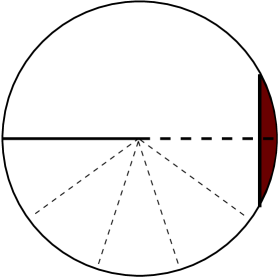
Figure 2: Schematic view of a Coleman-De Luccia bounce, with the coordinate $\xi$ running horizontally, from $\xi=0$ on the right to $\xi_{\rm max}$ on the left. As in Fig. 1, the shaded region represents the region of approximate true vacuum and the unshaded region that of approximate false vacuum. A path through configuration space, starting from the solid horizontal line and ending on the heavy dashed line, is given by the lighter dashed lines. Each of these lines represents a horizon volume that is topologically a three-ball with its center at the edge of the figure and its two-sphere horizon boundary at the center of the figure.

The fact that the bounce topology is compact raises questions: Why is the volume finite? How can the bounce be understood as a sequence of configurations forming a tunneling path through a potential energy barrier? It was argued in Brown:2007sd that the bounce should be understood as mediating a transition in a de Sitter horizon volume (giving a finite three-volume $\sim H^{-3}$) at a finite de Sitter temperature $T_{\rm dS}=H/2\pi$ (giving periodicity $\sim H^{-1}$ in a fourth Euclidean coordinate). In this picture the path through configuration space is given by a series of radial slices, each of which represents a three-dimensional ball, as shown in Fig. 2 (see also Tanaka:1992zw ). The boundaries of the various three-balls, which are two-spheres at the horizon, all meet and are identified. The initial and final slices are the two horizontal slices in this figure. In the non-gravitational case, the bounce connects initial and final configurations that are each turning points, with vanishing derivatives with respect to the Euclidean time, that can be continued to real time configurations with vanishing time derivatives. With gravitational effects included, the initial and final slices each correspond to a configuration on a horizon volume with instantaneously static metric and scalar field. In Appendix A we verify explicitly that these limiting configurations are indeed bounded by horizons.

III Negative modes

The occurrence of a negative eigenvalue in the spectrum of fluctuations about the bounce was an essential ingredient in the path integral derivation of the flat-space nucleation rate. It gave rise to the factor of $i$ in Eq. (10), which led to the bounce terms being a contribution to the imaginary part of the false vacuum energy.

The existence of the negative mode is readily established in flat spacetime. An O(4)-symmetric bounce obeys

$${d^{2}\phi\over ds^{2}}+{3\over s}{d\phi\over ds}=U^{\prime}(\phi)\,,$$ (39)

where $s=\sqrt{\tau^{2}+{\bf r}^{2}}$. The eigenmodes about this bounce satisfy

$$\left[-\Box_{E}+U^{\prime\prime}(\phi_{b})\right]\eta=\lambda\eta\,.$$ (40)

The spherical symmetry of the underlying bounce allows us to decompose the modes as products of a radial function and a four-dimensional spherical harmonic, and to recast Eq. (40) into the form of a Schroedinger equation, with the angular derivatives giving rise to an angular momentum barrier term. We know that the breaking of translational invariance gives rise to four zero modes that transform as the components of a four-dimensional vector. Standard arguments then show that there must be a rotationally invariant scalar mode with a lower, and therefore negative, eigenvalue $\lambda$ that obeys

$$-{d^{2}\eta\over ds^{2}}-{3\over s}{d\eta\over ds}+U^{\prime\prime}(\phi_{b})\eta=\lambda\eta\,.$$ (41)

This is readily verified for the case of a thin-wall bounce with radius $\bar{R}$. Differentiating Eq. (39) with respect to $s$ gives

$$\left[-{d^{2}\over ds^{2}}-{3\over s}{d\over ds}+U^{\prime\prime}(\phi_{b})\right]{d\phi_{b}\over ds}=-{3\over s^{2}}{d\phi_{b}\over ds}\,.$$ (42)

In the thin-wall limit $d\phi/ds$ vanishes except in a narrow region where $s\approx\bar{R}$, and so we see that there is an eigenfunction $\eta(s)\approx d\phi/ds$ with negative eigenvalue $\lambda\approx-3/\bar{R}^{2}$.

What about multiple negative modes? The determinant factor would acquire a factor of $i$ for each such mode, and so would be real if there were an even number of negative modes. Three such modes would give an imaginary determinant factor, but with the wrong sign. Although five modes, or any larger number equal to $1\mod 4$, would give an imaginary part of the right sign, this would seem to be an unusual constraint on the bounce.

The situation was clarified by Coleman Coleman:1987rm , who showed that if a bounce has multiple negative modes then the corresponding tunneling path through configuration space is a saddle point, rather than a minimum, of the barrier penetration integral. As an explicit illustration of this, consider a theory with a single scalar field whose potential has three minima, at $\phi_{A}<\phi_{B}<\phi_{C}$, of increasing depth, $U_{A}>U_{B}>U_{C}$ Tye:2009rb . It is convenient to choose the zero of energy so that $U_{A}=0$. Let us assume that the energy density differences

$$\epsilon_{1} \equiv U_{A}-U_{B}\,,$$ (43)

$$\epsilon_{2} \equiv U_{B}-U_{C}\,,$$ (44)

and the corresponding surface tensions $\sigma_{1}$ and $\sigma_{2}$ are such that the thin-wall approximation is valid for both the A-to-B and the B-to-C transitions. The corresponding thin-wall bubble radii are

$$\bar{R}_{j}={3\sigma_{j}\over\epsilon_{j}}\,,\qquad j=1,2\,.$$ (45)

Now consider a “double-bounce” configuration in which a spherical C-vacuum region of radius $R_{2}$ is centered within a spherical B-vacuum region of radius $R_{1}$, which itself is surrounded by an A-vacuum background. This is clearly a solution of the Euclidean field equations if $R_{1}=\bar{R}_{1}$ and $R_{2}=\bar{R}_{2}$. It is also clear that there are two negative modes, corresponding to independent variations of $R_{1}$ and $R_{2}$.

With a single spherical thin-wall configuration $\bar{R}$ is the unique radius consistent with having the four-dimensional fields interpolate between the false vacuum, at $\tau=-\infty$, and a three-dimensional configuration of equal energy containing a single bubble, at $\tau=0$. With two nested three-spheres there is a one-parameter family of configurations satisfying this equal energy condition, with their radii constrained to obey

$$0=4\pi\sigma_{1}R_{1}^{2}-{4\pi\over 3}\epsilon_{1}R_{1}^{3}+4\pi\sigma_{2}R_{2}^{2}-{4\pi\over 3}\epsilon_{2}R_{2}^{3}\,.$$ (46)

For each choice of $R_{1}$ and $R_{2}$ obeying this condition one can calculate the potential energy

$$V(\tau)=\int d^{3}x\left[\frac{1}{2}({\bm{\nabla}}\phi)^{2}+U(\phi)\right]$$ (47)

as a function of $\tau$ and then calculate the field theory generalization of the barrier penetration integral of Eq. (2). As expected, this has a minimum when $R_{2}=0$ and $R_{1}=\bar{R}_{1}$ (i.e. the ordinary A-to-B bounce). On the other hand, the choice $R_{1}=\bar{R}_{1}$ and $R_{2}=\bar{R}_{2}$ that gives the double-bounce solution turns out to maximize this tunneling integral. Thus, we would not expect this double-bounce solution to correspond, even with a reduced rate, to a new mode of bubble nucleation.

However, suppose that the parameters are such that the preferred radius, $\bar{R}_{2}$, of the B-to-C bounce is much less than $\bar{R}_{1}$. There will then be solutions in which a single A-to-B bounce contains many B-to-C bounces. In evaluating the path integral, we would then have to sum not only over all numbers of A-to-B bounces, as in Eq. (14), but also over the numbers of B-to-C bounces within each of these bubbles. This would lead to a double sum formula

$$I = I_{0}\sum_{n=0}^{\infty}{1\over n!}\,\left[i\Omega TK_{1}e^{-B_{1}}\sum_{k=0}{1\over k!}\left(i{\cal V}_{4}K_{2}e^{-B_{2}}\right)^{k}\right]^{n}$$ (48)

$$= I_{0}\sum_{n=0}^{\infty}{1\over n!}\,\left[i\Omega TK_{1}e^{-B_{1}}\sum_{k=0}{1\over k!}\left({i\over 2}\,{\cal V}_{4}\Gamma_{2}\right)^{k}\right]^{n}\,,$$ (49)

where

$${\cal V}_{4}={81\pi^{2}\over 2}\,\left(\sigma\over\epsilon\right)^{4}$$ (50)

is the four-volume of the A-to-B bounce and $\Gamma_{2}$ is the bubble nucleation rate for the B-to-C transition. Because $\Omega T$ is understood to be eventually taken to infinity, the upper limit on the sum over $n$ can be taken to be infinity, allowing us to convert the sum to an exponential. By contrast, ${\cal V}_{4}$ is fixed and finite, leading us to consider two regimes. If ${\cal V}_{4}\Gamma_{2}$ is much less than unity, the sum over $k$ is dominated by the $k=0$ term, the A-to-B bounces containing B-to-C sub-bounces can be ignored, and there is no significant correction to $\Gamma_{1}$. On the other hand, if ${\cal V}_{4}\Gamma_{2}$ is much greater than unity, the sum over $k$ can be approximated by an exponential, which has the effect of replacing $B_{1}$ by Czech:2011aa

$$\tilde{B}_{1}=B_{1}-{i\over 2}{\cal V}_{4}\Gamma_{2}={27\pi^{2}\over 2}\,{\sigma_{1}^{4}\over\epsilon_{1}^{3}}\left(1-{3i\over 2}\,{\Gamma_{2}\over\epsilon_{1}}\right)\,.$$ (51)

To leading order, this is the same as making the replacement $\epsilon_{1}\rightarrow\epsilon_{1}+i\Gamma_{2}/2$ or, in other words, as if we had given the energy density of vacuum B an imaginary part $\Gamma_{2}/2$. This describes a situation in which vacuum B is sufficiently unstable that bubbles of B already contain tiny bubbles of C at the time that they nucleate. Thus, although though the double-bounce with two negative modes has little physical relevance, the solutions with many sub-bounces and hence many negative modes are physically meaningful. Although they have a somewhat higher action than the unadorned single bounce, this is outweighed by the fact that they are more numerous. In essence, it is a case of “entropy” overcoming “energy”.

IV Perturbative expansion about a CDL bounce

In this section we consider the expansion of the Euclidean action about an O(4)-symmetric bounce solution of Eqs. (30) and (31), and obtain the contribution from the terms quadratic in fluctuations about the bounce. We require that these fluctuations obey the constraints that follow from the freedom to make coordinate transformations. To exclude fluctuations that are purely coordinate transformations, we write the quadratic action in terms of explicitly gauge-invariant quantities.

It is convenient to exploit the O(4) symmetry by expanding the fluctuations in terms of O(4) harmonics. The normal modes can be classified as scalar, vector, or tensor. Because the only matter source is a scalar field, it suffices for us to focus on the scalar modes. We begin by considering the most important case, the O(4)-symmetric zero angular momentum modes.

IV.1 O(4)-symmetric fluctuations

With O(4) symmetry retained, we can write the metric as

$$ds^{2}=[1+2A(\xi)]d\xi^{2}+\rho(\xi)^{2}[1+2\Psi(\xi)]d\Omega_{3}^{2}\,,$$ (52)

corresponding to the perturbations

$$N(\xi) \rightarrow 1+A(\xi)\,,$$ (53)

$$\rho(\xi) \rightarrow \rho(\xi)[1+\Psi(\xi)]\,,$$ (54)

and define the perturbed scalar field

$$\phi(\xi)\rightarrow\phi(\xi)+\Phi(\xi)\,.$$ (55)

Next we expand the total action about the background solution. The first-order correction to the action vanishes by the background equations of motion. The quadratic terms are given by

$$S^{(2)}_{E}=2\pi^{2}\int L^{(2)}_{E}(\Phi,\Psi,A;\dot{\Phi},\dot{\Psi})d\xi\,,$$ (56)

where

$$L^{(2)}_{E}(\Phi,\Psi,A;\dot{\Phi},\dot{\Psi})=-\frac{3}{\kappa}\rho^{3}\dot{\Psi}^{2}+\frac{3}{\kappa}\rho\Psi^{2}+\frac{1}{2}\rho^{3}\dot{\Phi}^{2}+\frac{1}{2}\rho^{3}U^{\prime\prime}\Phi^{2}-3\rho^{3}\dot{\phi}\dot{\Psi}\Phi\,$$ (57)

$$+\left(-\rho^{3}\dot{\phi}\dot{\Phi}+\rho^{3}U^{\prime}\Phi+\frac{6}{\kappa}\dot{\rho}\rho^{2}\dot{\Psi}+\frac{6}{\kappa}\rho\Psi\right)A-\frac{3}{\kappa}\rho QA^{2}\,.$$ (58)

Here we have defined

$$Q=\left(1-{\kappa\rho^{2}U\over 3}\right)=\dot{\rho}^{2}-\frac{\kappa\rho^{2}\dot{\phi}^{2}}{6}\,,$$ (59)

with the two expressions being equal because of Eq. (30).

The theory is invariant under coordinate transformations. For perturbations about a background solution, the coordinate transformation $\xi\rightarrow\xi+\alpha(\xi)$ gives the infinitesimal gauge transformation

$$\delta_{G}\Phi=\dot{\phi}\alpha,\quad\delta_{G}\Psi=\frac{\dot{\rho}}{\rho}\alpha,\quad\delta_{G}A=\dot{\alpha}\,.$$ (60)

This leaves $L_{E}^{(2)}$ unchanged, up to a total derivative (see Appendix B), and so is an invariance of the action.

Closely related to this gauge invariance is the existence of a constraint that follows from the fact that $L^{(2)}_{E}$ does not contain derivatives of $A$. Requiring that $\delta L^{(2)}_{E}/\delta A$ vanish gives

$$0={\cal C}^{(1)}\equiv\frac{\kappa\rho^{2}}{6}\left(\dot{\phi}\dot{\Phi}-U^{\prime}\Phi\right)-\left(\rho\dot{\rho}\dot{\Psi}+\Psi\right)+QA\,.$$ (61)

This is nothing more than the linear term in the expansion of the constraint arising from the variation $N(\xi)$, and could have been obtained by substituting Eqs. (54) and (55) into Eq. (29). Using this constraint we can eliminate $A$ from Eq. (58). After some tedious calculations, described in Appendix B, we obtain the remarkably simple expression

$$L^{(2)}_{E}(\chi;\dot{\chi})=\frac{\rho^{3}}{2Q}\dot{\chi}^{2}+\frac{\rho^{3}}{2Q}f(\rho,\phi)\chi^{2}\,,$$ (62)

where we have defined the gauge-invariant quantity

$$\chi\equiv\dot{\rho}\Phi-\rho\dot{\phi}\Psi$$ (63)

and

$$f(\rho,\phi)=U^{\prime\prime}+\frac{\kappa\rho^{2}U^{\prime 2}}{3Q}+\frac{\kappa\rho\dot{\phi}U^{\prime}}{3\dot{\rho}Q}+\frac{2\kappa\dot{\phi}^{2}}{3}-\frac{\kappa\rho\dot{\phi}U^{\prime}}{\dot{\rho}}-\frac{4\kappa U}{3}-{\ddot{\rho}\dot{Q}\over\dot{\rho}Q}\,.$$ (64)

Our expression for the second-order Lagrangian $L^{(2)}_{E}$ is now manifestly gauge-invariant. One can check that the constraint ${\cal C}^{(1)}$ is likewise gauge-invariant.

IV.2 Non-spherically-symmetric perturbations

The O(4)-symmetric perturbations of the metric are completely described by the two functions $A$ and $\Psi$. Less symmetric perturbations require additional fields. For arbitrary angular momentum the perturbed metric can be written as

$$ds^{2} = [1+2A_{l}(\xi)Y_{l}(\Omega)]\,d\xi^{2}+B_{l}(\xi)\nabla_{a}Y_{l}(\Omega)\,d\xi\,dz^{a}\,$$ (66)

$$+\rho(\xi)^{2}\left\{\bar{g}_{ab}[1+2\Psi_{l}(\xi)Y_{l}(\Omega)]+2C_{l}(\xi)k^{-2}\left(\nabla_{a}\nabla_{b}+\frac{k^{2}}{3}\bar{g}_{ab}\right)Y_{l}(\Omega)\right\}dz^{a}dz^{b}\,.$$

Here $\bar{g}_{ab}$ is the standard round metric on the three-sphere with coordinates $z^{a}$ and $\nabla_{a}$ is the corresponding covariant derivative. The spherical harmonics $Y_{l}(\Omega)$ are eigenfunctions of the Laplacian on the three-sphere, with

$$\Delta Y_{l}(\Omega)=-l(l+2)\,Y_{l}(\Omega)=-k^{2}\,Y_{l}(\Omega)\,.$$ (68)

For simplicity of notation we have defined $k^{2}=l(l+2)$ and have suppressed the indices corresponding to the $(l+1)^{2}$ degeneracy of the modes and spherical harmonics of angular momentum $l$. In the following we will also omit the subscript $l$ on the harmonics and the coefficient functions.

For $l=k=0$, the quantities multiplying $B$ and $C$ vanish, and Eq. (LABEL:generalPertMetric) reduces to our previous expression, Eq. (52). If $l=1$, and thus $k^{2}=3$, the quantity multiplying $C$ vanishes as a result of the identity

$$\partial_{a}\partial_{b}Y_{1m}(\Omega)=-\bar{g}_{ab}Y_{1m}(\Omega)$$ (69)

and there are only three metric coefficients, $A$, $B$, and $\Psi$.

Expanding to second order in these perturbations gives the quadratic Lagrangian

$$L^{(2)}_{E} = -\frac{3}{\kappa}\rho^{3}\dot{\Psi}^{2}-\frac{\rho}{\kappa}(k^{2}-3)\Psi^{2}+\frac{1}{2}\rho^{3}\dot{\Phi}^{2}+\frac{1}{2}\left(k^{2}\rho+\rho^{3}U^{\prime\prime}\right)\Phi^{2}-3\rho^{3}\dot{\phi}\dot{\Psi}\Phi\,$$ (73)

$$+\frac{\rho^{3}}{3\kappa}\left(\frac{k^{2}-3}{k^{2}}\right)\dot{C}^{2}-\frac{\rho}{9\kappa}(k^{2}-3)C^{2}-\frac{2\rho}{3\kappa}(k^{2}-3)\Psi C\,$$

$$+\left[-\rho^{3}\dot{\phi}\dot{\Phi}+\rho^{3}U^{\prime}\Phi+\frac{6}{\kappa}\dot{\rho}\rho^{2}\dot{\Psi}+\frac{6}{\kappa}(1-k^{2}/3)\rho\Psi+\frac{2}{\kappa}(1-k^{2}/3)\rho C\right]A-\frac{3}{\kappa}\rho QA^{2}\,$$

$$+\frac{2\dot{\rho}k^{2}}{\kappa}AB-\left[\frac{2\rho}{\kappa}\dot{\Psi}+\frac{2\rho}{3\kappa}\left(\frac{k^{2}-3}{k^{2}}\right)\dot{C}+\rho\dot{\phi}\Phi\right]k^{2}B-\frac{k^{2}}{\kappa\rho}B^{2}\,.$$

This Lagrangian is invariant under the two-parameter coordinate transformation

$$\xi \rightarrow \xi+\alpha(\xi)Y(\Omega)\,,$$ (74)

$$z_{a} \rightarrow z_{a}+\beta(\xi)\partial_{a}Y(\Omega)\,,$$ (75)

under which the perturbations transform as

$$\delta_{G}\Phi=\dot{\phi}\alpha,\quad\delta_{G}\Psi=\frac{\dot{\rho}}{\rho}\alpha-\frac{k^{2}}{3}\beta,\quad\delta_{G}A=\dot{\alpha},\quad\delta_{G}B=\alpha+\rho^{2}\dot{\beta},\quad\delta_{G}C=k^{2}\beta\,.$$ (76)

With two independent gauge parameters $\alpha$ and $\beta$ we expect to have two constraints. Indeed, we see that no derivatives of $A$ or $B$ appear in $L^{(2)}$. Differentiating with respect to these quantities leads to the constraints

$$0={\cal C}^{(1)}_{A}\equiv\frac{\kappa\rho^{2}}{6}\left(\dot{\phi}\dot{\Phi}-U^{\prime}\Phi\right)-\left[\rho\dot{\rho}\dot{\Psi}+\left(1-\frac{k^{2}}{3}\right)\left(\Psi+\frac{C}{3}\right)+\frac{\dot{\rho}k^{2}}{3\rho}B\right]+QA$$ (77)

and

$$0={\cal C}^{(1)}_{B}\equiv\dot{\Psi}+\frac{k^{2}-3}{3k^{2}}\dot{C}+\frac{\kappa\dot{\phi}}{2}\Phi-\frac{\dot{\rho}}{\rho}A+\frac{1}{\rho^{2}}B=0\,.$$ (78)

Both of these constraints are gauge-invariant, leading us to again seek a manifestly gauge-independent form of the Lagrangian. Using the constraints to eliminate $A$ and $B$ and proceeding as before, we obtain

$$L^{(2)}_{E}=\frac{\rho^{3}(1-k^{2}/3)}{2(Q-\dot{\rho}^{2}k^{2}/3)}\dot{\chi}^{2}+\frac{\rho^{3}(1-k^{2}/3)}{2(Q-\dot{\rho}^{2}k^{2}/3)}f(\rho,\phi)\chi^{2}\,,$$ (79)

where now $\chi$ is the only possible gauge-invariant generalization of Eq. (63),

$$\chi\equiv\dot{\rho}\Phi-\rho\dot{\phi}\Psi-\frac{\rho\dot{\phi}}{3}C\,,$$ (80)

and

$$f = U^{\prime\prime}+{k^{2}\over\rho^{2}}+\frac{\kappa}{3\dot{\rho}(Q-\dot{\rho}^{2}k^{2}/3)}\left\{\rho\dot{\phi}U^{\prime}+\rho^{2}\dot{\rho}U^{\prime 2}-k^{2}\left[2\rho\dot{\rho}^{2}\dot{\phi}U^{\prime}-3\dot{\rho}\dot{\phi}^{2}Q+\dot{\rho}\dot{\phi}^{2}\right]\right\}$$ (82)

$$\qquad+\frac{2\kappa\dot{\phi}^{2}}{3}-\frac{\kappa\rho\dot{\phi}U^{\prime}}{\dot{\rho}}-\frac{4\kappa U}{3}-{\ddot{\rho}\over\dot{\rho}}\left({\dot{Q}-2\dot{\rho}\ddot{\rho}k^{2}/3\over Q-\dot{\rho}^{2}k^{2}/3}\right)\,.$$

If $l=k=0$, Eq. (79) reduces to the result of the previous subsection. For $l=1$ and $k^{2}=3$, $L^{(2)}_{E}$ vanishes identically. Finally, note that the coefficient of $\dot{\chi}^{2}$ is positive for all $l\geq 2$.

IV.3 Perturbations about a homogeneous solution

The analysis of the previous two subsections is modified somewhat if the unperturbed solution is homogeneous, with $\phi$ constant and equal to an extremum of $U(\phi)$ and the metric being the usual round metric on the four-sphere. This could be the false vacuum solution given by Eqs. (33) and (34) or the analogous true vacuum solution, in either case with $U^{\prime\prime}>0$. Alternatively, it could be the Hawking-Moss solution Hawking:1981fz with $\phi=\phi_{\rm HM}$ at a local maximum of $U$.

If we examine the quadratic Lagrangians in Eqs. (58) and (73), we see that the terms coupling $\Phi$ with a metric perturbation are all absent if $\dot{\phi}$ and $U^{\prime}$ both vanish. Furthermore, $\Phi$ drops out of the constraints, and $Q$ is identically equal to unity. Finally, $\chi$ is simply $\Phi$. Redoing the analysis, we find that the metric terms are removed by the constraints, and we obtain simply

$$L^{(2)}_{E}=\frac{1}{2}\rho^{3}\left[\dot{\Phi}^{2}+\left(U^{\prime\prime}+{k^{2}\over\rho^{2}}\right)\Phi^{2}\right]\,.$$ (83)

(Note that the $l=1$ modes do not drop out, in contrast with the perturbations about inhomogeneous bounces.) The eigenmodes of this Lagrangian are just the five-dimensional spherical harmonics. If

$$\frac{U^{\prime\prime}}{H_{\rm top}^{2}}<-N(N+3)$$ (84)

with $N=0,1,\dots$, then there are $N+1$ negative eigenvalues. If these are numbered $n=0,1,\dots$, eigenvalue $n$ has a degeneracy $(2n+3)(n+2)(n+1)/6$.

V Negative modes with gravity

In this section we investigate the $\chi$-field modes with negative eigenvalues that arise from the quadratic Euclidean actions that were obtained in Sec. IV. These actions, given in Eqs. (62) and (79), are comprised of a “kinetic energy” term quadratic in $\dot{\chi}$ and a “potential energy” term quadratic in $\chi$. For $l=0$ the kinetic energy can be either positive or negative, depending on the sign of $Q$, while the sign of the potential energy is that of $f/Q$. For $l\geq 2$ the kinetic energy is always positive and the sign of the potential energy is that of $f$. (As already noted, there are no gauge-invariant modes for $l=1$.)

We can distinguish two classes of negative modes:

a) Slowly varying or “standard” negative modes: These are associated with a positive kinetic energy and a negative potential energy. They are the analogues of the negative mode about the flat-space bounce. We will restrict our investigation to the $l=0$ case; although we do not expect negative modes with higher $l$ (there are none in flat spacetime), we have not been able to prove that these are impossible.

b) Rapidly oscillating modes: These arise if $l=0$ and $Q<0$, giving a negative kinetic energy. Low-amplitude, short-wavelength oscillations of the form $\chi\sim\sin(\omega\xi)/\omega$ in the region of negative $Q$ can yield modes with negative eigenvalues whose magnitudes grow without bound as $\omega$ tends toward infinity; this is a manifestation of the conformal mode problem of Euclidean gravity Gibbons:1978ac .

We will consider these two cases separately.

V.1 Slowly varying negative modes

In flat spacetime these are associated with the variation of the bubble radius $R$. Indeed, in the thin-wall approximation, they are signaled by the fact that $d^{2}S_{E}/dR^{2}$ is negative at $R=\bar{R}$, as noted in Eq. (22). As has already been noted, when the thin-wall approximation is applied to the case with gravitational effects included, one finds that for a bubble with a wall at $\rho=\bar{\rho}$ the second derivative $d^{2}S_{E}/d\bar{\rho}^{2}$ is negative for a type A de Sitter bounce, but positive for a type B bounce. This suggests that there is a slowly-varying negative mode in the former case, but not in the latter.

To study this issue further, and going beyond the thin-wall limit, we took as an example a theory with a scalar field potential,

$$U(\phi)=(\phi-3)^{2}\phi^{2}+0.5\phi^{2}+1.5\,,$$ (85)

whose false and true vacua are at $\phi=2.81$ and $\phi=0$, respectively. We studied the behavior of the bounce solutions as the strength of gravity was progressively increased. We worked with a dimensionless $\phi$ and $\kappa$; the translation to physical quantities is obtained by noting that for this potential the scalar field mass scale $\mu$, defined in Eq. (36), is related to the Planck mass by

$${\mu\over M_{\rm Pl}}=0.24\sqrt{\kappa}\,.$$ (86)

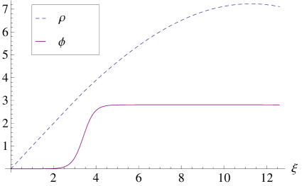
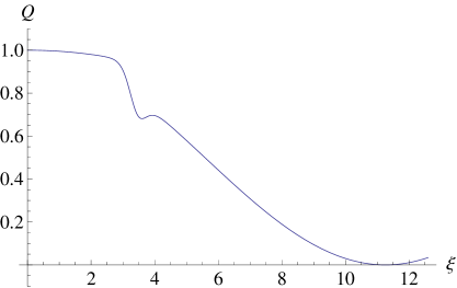
(a)                                                                   (b)

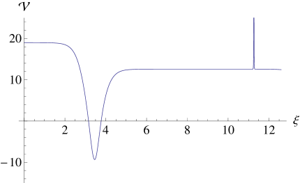
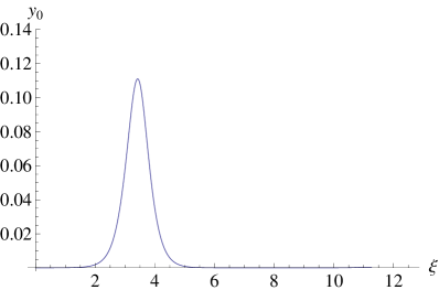
(c)                                                                   (d)

Figure 3: Results for the potential given in Eq. (85), with $\kappa=0.01$. The bounce solution is shown in (a), with $\rho$ given by the dashed blue line and $\phi$ by the solid red line. Panel (b) shows $Q$. The minimum at the location of the maximum of $\rho$ is negative, although this is not apparent in the figure due to its exponentially small absolute value. Panel (c) shows the function ${\cal V}$ given in Eq. (89). The lowest eigenmode of the Lagrangian of Eq. (88) is shown in (d); its eigenvalue is $-(0.40\mu)^{2}$.

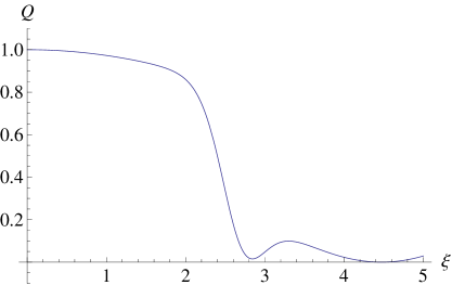
(a)                                                                   (b)

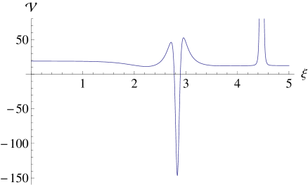
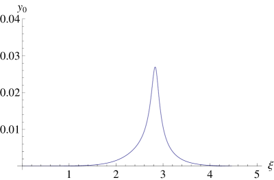
(c)                                                                   (d)

Figure 4: The same as in Fig. 3, but for $\kappa=0.055$. At the first minimum $Q=0.015$, while at the second it has an exponentially small negative value. The eigenvalue of the negative mode is $-(0.21\mu)^{2}$.

To make the comparison with the flat-space case clearer we define

$$y=\chi/\sqrt{Q}$$ (87)

and rewrite Eq. (62) as

$$L^{(2)}_{E}={\rho^{3}\over 2}\left(\dot{y}^{2}+{\cal V}y^{2}\right)\,,$$ (88)

with

$${\cal V}=U^{\prime\prime}+{\kappa\rho^{2}{U^{\prime}}^{2}\over 3Q}+{\kappa\rho\dot{\phi}U^{\prime}\over 3\dot{\rho}Q}-{3\dot{\rho}\dot{Q}\over 2\rho Q}-{\ddot{Q}\over 2Q}+{3\dot{Q}^{2}\over 4Q^{2}}+{3\ddot{\rho}\over\rho}+{\dddot{\rho}\over\dot{\rho}}-{\ddot{\rho}\dot{Q}\over\dot{\rho}Q}\,.$$ (89)

Figures 3 - 7 show the evolution of the bounce and the lowest eigenmode as the gravitational coupling $\kappa$ is increased. In Fig. 3 we show the bounce fields $\phi(\xi)$ and $\rho(\xi)$ for the weak gravity case $\kappa=0.01$ (i.e., $\mu=0.024M_{\rm Pl}$). The bubble wall is located well before the maximum of $\rho$, so this is clearly a type A bounce, and might almost be classified as a small-bubble bounce. The dominant term in ${\cal V}$ is $U^{\prime\prime}$, as in flat space. The negative mode is concentrated on the wall region of the bounce. Its eigenvalue is $\lambda_{0}=-(0.40\mu)^{2}$, which can be compared with the flat-space ($\kappa=0$) value $-(0.39\mu)^{2}$. There is a second minimum of $Q$ at the value of $\xi$ where $\rho$ reaches its maximum. From Eq. (59) we see that $Q$ is negative there, although the factor of $\dot{\phi}^{2}$ makes its absolute value exponentially small. We will return to this minimum and the narrow region of negative $Q$ surrounding it in the next subsection.

Increasing the strength of gravity to $\kappa=0.055$ (i.e., $\mu=0.056M_{\rm Pl}$) yields the results shown in Fig. 4. The maximum of $\rho$ is outside the bubble wall (although just barely so), and so this is a large type A bounce. $Q$ remains positive throughout the wall region, although it reaches a minimum value of 0.015 near the center of the bubble wall. Gravitational effects have significantly modified ${\cal V}$, whose negative region is much narrower. The negative mode has become somewhat narrower, but as before it is centered about the minimum of $Q$ in the wall. The eigenvalue has increased to $-(0.21\mu)^{2}$.

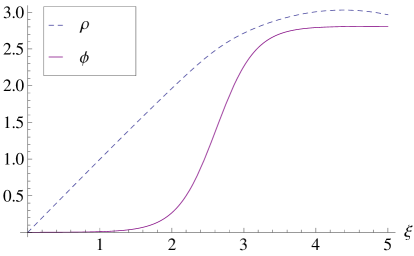
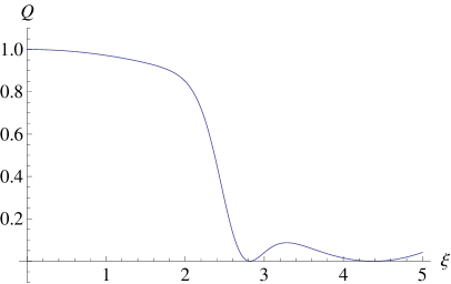
(a)                                                                   (b)

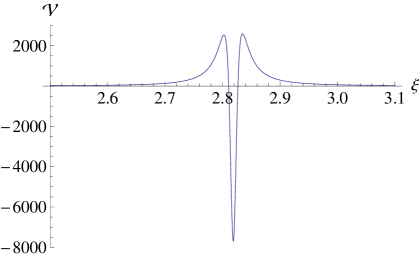
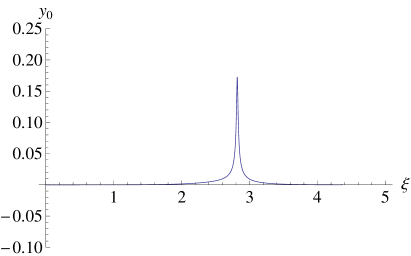
(c)                                                                   (d)

Figure 5: Results for $\kappa=0.057$. The plots are analogous to those in Fig. 4, except that in (c) the plot covers only a narrow range of $\xi$ containing the dip in ${\cal V}$. Outside this range ${\cal V}$ shows little change from Fig. 4. Again $Q$ has two minima, one positive and one negative; at the former $Q=0.00027$. The lowest eigenmode, shown in (d), has a positive eigenvalue $(0.23\mu)^{2}$.

The effect of a further increase in $\kappa$, to 0.057 (and, by a numerical coincidence, $\mu=0.057M_{\rm Pl}$), is shown in Fig. 5. The profiles of $\rho$ and $\phi$ show little change, and the bounce remains type A. The minimum value of $Q$ in the wall remains positive, at 0.00027. The dip in ${\cal V}$ is now much deeper and much narrower. Most importantly, the lowest eigenvalue is now positive, at $(0.23\mu)^{2}$, even though this is still a type A bounce.

With even a slight further increase of $\kappa$, the minimum value of $Q$ on the bubble wall becomes negative. This is illustrated in Fig. 6 for the case $\kappa=0.07$ ($\mu=0.063M_{\rm Pl}$). Because the change of variables from $\chi$ to $y$ can no longer be carried out, $\cal V$ ceases to be a useful quantity, and there is no analogue of the lowest eigenmodes of the previous examples. If there is a slowly varying negative mode, it is not simply related to the ones found in type A solutions with weaker gravity and smaller bounces.

With $\kappa$ increased to 0.09 ($\mu=0.072M_{\rm Pl}$), we have a bounce, shown in Fig. 7, that can be viewed as being on the borderline between type A to type B. We see that the regions of negative $Q$ at the wall and at $\rho_{\rm max}$ have merged to form a single negative-$Q$ region.

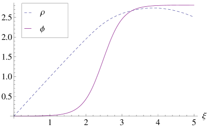
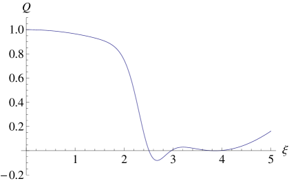
(a)                                                                   (b)

Figure 6: Results for $\kappa=0.07$. Panels (a) and (b) are as in Fig. 3. Note that $Q$ now has two negative regions.

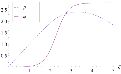
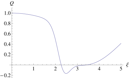
(a)                                                                   (b)

Figure 7: Same as for Fig. 6, but for $\kappa=0.09$. The regions of negative $Q$ have now merged to form a single connected region.

Finally, in Fig. 8 we illustrate a clear-cut type B bounce. Instead of Eq. (85), the potential is now given by

$$U=10(\phi^{2}-0.25)^{2}+0.1(\phi+1)\,.$$ (90)

The plots are for $\kappa=1$, corresponding to $\mu/M_{\rm Pl}=0.17$. The potential ${\cal W}=f/Q$ is everywhere positive, so there is no possibility of a standard slowly varying negative mode.

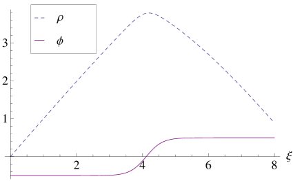
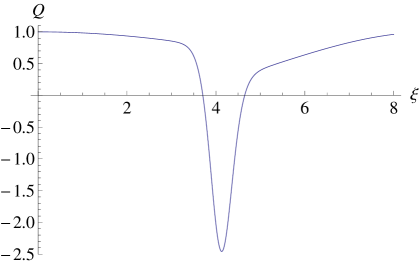
(a)                                                                   (b)

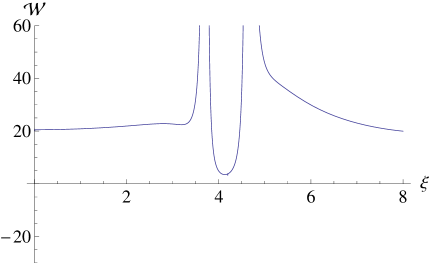
(c)

Figure 8: A type B bounce, with $\kappa=1$ and the potential given by Eq. (90). Panels (a) and (b) are as in Fig. 6, while panel (c) shows ${\cal W}=f/Q$.

V.2 Rapidly oscillating modes

These arise whenever $Q$, defined by Eq. (59), is negative; i.e., whenever

$${\kappa\rho^{2}\dot{\phi}^{2}\over 6\dot{\rho}^{2}}>1\,.$$ (91)

This can happen in two different situations. For some bounces, $Q$ becomes negative in a portion of the bubble wall, leading to what we will call “wall modes”; we saw an example of this in Fig. 6. For all bounces arising from de Sitter space, $Q$ becomes negative in a region about the maximum of $\rho$; the resulting negative modes may be called “$\rho_{\rm max}$ modes”. Of course, the distinction between these classes only applies for type A bounces; for type B bounces, where $\rho_{\rm max}$ is reached in the bubble wall, the distinction disappears. Indeed, Fig. 7 illustrates how the two classes merge as type A crosses over to type B.

We start by considering a small bubble bounce, with $\mu\ll M_{\rm Pl}$ and the bubble radius $\bar{\rho}\ll H^{-1}$. In the wall region $\dot{\phi}^{2}\sim\mu^{4}$, while $\dot{\rho}\approx 1$, so

$${\kappa\rho^{2}\dot{\phi}^{2}\over 6\dot{\rho}^{2}}\sim{\mu^{4}\bar{\rho}^{2}\over M_{\rm Pl}^{2}}\,.$$ (92)

For a typical small bubble bounce this is much less than unity, and so there are no wall modes.

There will, however, be $\rho_{\rm max}$ modes. These will be centered about $\xi=(\pi/2H)-\Delta\equiv\xi_{0}$, where $\rho$ reaches its maximum. From Eq. (37) we find that in this region $\rho\approx H^{-1}$ and

$$\dot{\rho}\approx\sin[H(\xi_{0}-\xi)]\approx H(\xi_{0}-\xi)\,,$$ (93)

while $\dot{\phi}$ is exponentially small, with $|\dot{\phi}|\sim\mu^{2}e^{-\mu\pi/2H}$. It follows that $Q$ is only negative in a region with an exponentially small width,

$$\Delta\xi\approx{\mu^{2}\over H^{2}M_{\rm Pl}}\,e^{-\mu\pi/2H}\,,$$ (94)

that is much less than a Planck length. As a result, the eigenvalues of the negative modes will all be super-Planckian.

We turn now to the case of a large type A bounce. In the thin-wall approximation this has $\rho\approx H_{t}^{-1}\sin(H_{t}\xi)$ in the true vacuum region. In order to have a region of negative $Q$, we need that at the wall

$${\kappa\rho^{2}\dot{\phi}^{2}\over 6\dot{\rho}^{2}}\sim{\mu^{4}\over H_{t}^{2}M_{\rm Pl}^{2}}\,\tan^{2}(H_{t}\bar{\xi})\sim{\mu^{4}\over U_{\rm tv}}\,\tan^{2}(H_{t}\bar{\xi})$$ (95)

be greater than unity. As we have already seen in Fig. 6, it is easy to construct examples where this is true without invoking any Planckian mass scales Lavrelashvili:1985vn .

These type A bounces will also have $\rho_{\rm max}$ modes, with support in a region of width

$$\Delta\xi\approx{\mu^{2}M_{\rm Pl}\over U_{\rm tv}}\,e^{-\mu(\xi_{0}-\xi)}\,.$$ (96)

Even for a large type A bounce, such as those illustrated in Figs. 4-6, where the wall is only a few e-foldings away from $\rho_{\rm max}$, this width remains small, although not necessarily sub-Planckian, almost until the point where the type A bounce goes over to type B.

For type B bounces, where $\rho$ reaches its maximum inside the bubble wall, the distinction between the two types of rapidly oscillating negative modes disappears; a typical example is illustrated in Fig. 8.

Table 1 summarizes the results of this section.

	Slowly varying	Wall oscillating	$\rho_{\rm max}$ oscillating
Small type A	Yes	No	Planckian
Large type A	Usually	Possible	Yes
Type B	No	—	Yes

Table 1: Summary of the results of Sec. V, indicating the types of negative modes that occur with the various classes of bounces. Note that for type B bounces there is no distinction between the two types of oscillating negative modes.

VI Negative modes about multibounce configurations

In discussions of tunneling in flat spacetime, one usually focuses on the single-bounce solution and its associated determinant factor and normal modes. In the usual dilute gas approximation, the deviation of the determinant from its value in the pure false vacuum can be approximated as being local to the bounce, so that for multibounce quasi-stationary points the determinant term, including its single factor of $i$, is simply repeated for each additional bounce. Summing over all numbers of bounces leads to an exponential, with the factor of $i$ promoted to the exponent.

The situation is more subtle with gravitational effects included. For large type A bounces (and of course for all type B bounces), there may not even be room on the Euclidean sphere to have several well-separated bounces. On the other hand, if the scalar field mass scale $\mu$ is far below the Planck mass and the bounce radius is much less than $H^{-1}$, there is no problem at all with configurations containing large numbers of component bounces. However, one wonders what becomes of the $\rho_{\rm max}$ negative modes, which are not localized about the bounce, when there are multiple bounces.

To start, consider an O(4)-symmetric solution with two bounces centered at antipodal points, which we may take to be $\xi=0$ and $\xi=\xi_{\rm max}$. There is potentially a negative-$Q$ region about the “equator” at $\xi=\xi_{\rm max}/2$. By symmetry, $\dot{\phi}=0$ here, so both terms in

$$Q=\dot{\rho}^{2}-{\kappa\rho^{2}\dot{\phi}^{2}\over 6}$$ (97)

vanish at the equator. If the bounces have radii much less than the horizon length, $\dot{\phi}$ will be exponentially small, $Q$ will be positive, and the infinite set of oscillating negative modes will be absent. On the other hand, with larger bounces one can easily find parameters that would make the first term smaller than the second in the region close to the equator, giving a negative $Q$ and a family of oscillating negative modes.

Having seen that two-bounce solutions may or may not have negative-$Q$ regions, let us turn to the more generic multibounce case, with many component small bounces. A schematic view of such a solution is shown in Fig. 9. Here the small circles represent the individual bounces, with $\phi$ close to its true vacuum value near their centers. As one moves away from one of these circles $\phi$ rapidly approaches $\phi_{\rm fv}$. Thus, in most of the space $|\phi-\phi_{\rm fv}|$ is exponentially small. The magnitude of this exponential tail decreases as the distance to the nearest bounce increases. Roughly speaking, this tail decreases in magnitude until one reaches the dotted lines in the figure, which schematically represent the boundaries that separate the “domains” of the individual bounces.

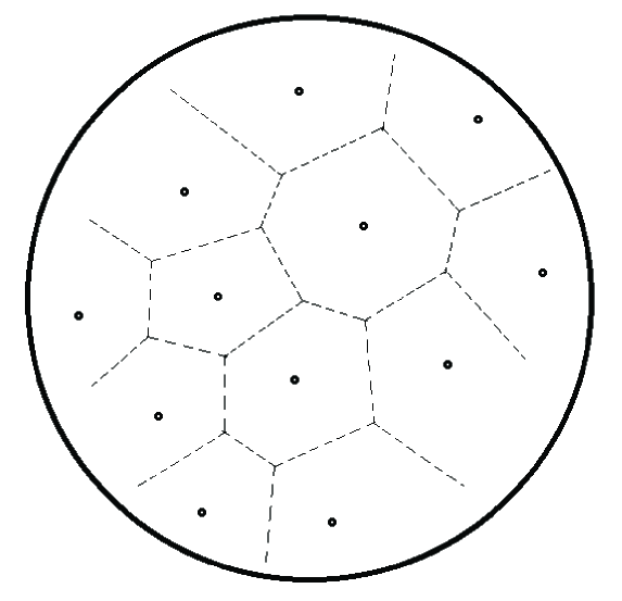
Figure 9: Schematic illustration of a many-bounce configuration.

Although we have no overall O(4) symmetry to guide us, we can look to our analysis of the single bounce case for guidance. We begin by remarking that the fields in the interior of each domain are, to a good approximation, the same as those in a region of comparable size about the bounce in a one-bounce solution. Since the rapidly oscillating negative modes in the one-bounce solution have support far from this region, we should not expect to find them in the domain interiors.

Hence, if rapidly oscillating negative modes exist, they should be located near the domain boundaries. However, even that seems quite unlikely. With many component bounces, the typical domain size is much smaller than the curvature radius of the underlying four-sphere. Thus, viewed on the scale of a few domains, the solution is barely distinguishable from the corresponding flat-space multibounce configuration, which we know has no oscillating negative modes. To phrase this differently, in the one-bounce solution the negative-$Q$ region is a thin three-sphere shell with a curvature radius equal to that of the four-sphere background. In the multibounce configuration the domain boundaries approximate thin three-sphere shells with curvature radii much smaller than that of the underlying background.

We conclude that while rapidly oscillating negative modes exist for the one-bounce solution, and possibly even for quasi-stationary points with a handful of bounces, they will be absent for configurations with many bounces. We need to ask ourselves which of these cases is the one of relevance for us.

In the discussion of tunneling in flat spacetime in Sec. II.1 we argued that the path integral was dominated by configurations with $n$ bounces, with $n$ given by Eq. (18). With a total four-volume of $\Omega T$, we had $n\sim(\Omega T)\Gamma$. Of course, the four-volume was understood to be taken to infinity at the end of the calculation, so the conclusion was that the path integral was dominated by configurations in which the bounces were infinite in number but with a finite density of the order of $\Gamma$.

If we ignore for the moment any complications from rapidly varying negative modes (which will, in any case, be absent if $n$ is large), then analogous reasoning leads to the conclusion that the dominant configurations for de Sitter tunneling should be ones with

$$n\approx\left({8\pi^{2}\over 3}\,H^{-4}\right)\left(Ke^{-B}\right)$$ (98)

component bounces. The first factor, ${8\pi^{2}\over 3}\,H^{-4}$, is the four-volume of the Euclidean de Sitter space. The second factor is (apart from a factor of 2) the usual expression for the nucleation rate per unit volume, $\Gamma$. Dimensional analysis suggests that

$$r\equiv{\Gamma\over H^{4}}\sim\left({M_{\rm Pl}\over\mu}\right)^{4}\,e^{-B}\,.$$ (99)

Depending on the parameters of the scalar field theory, this ratio could easily be much less than or much greater than unity; given the exponential dependence on the bounce action, obtaining a value very close to unity, while possible, is unlikely.

If $r\gg 1$ the path integral is overwhelmingly dominated by configurations with many bounces. These configurations have only the usual slowly varying negative modes, one for each bounce. The anomalous rapidly varying negative modes are absent. On the other hand, if $r\ll 1$ the contributions from multibounce configurations are negligible, and the single-bounce solution, with its infinite set of negative modes, makes the important contribution to the path integral.

VII Discussion and summary

In examining various CDL bounces, we have found patterns of negative modes that are rather different from those encountered in the absence of gravity. It seems natural to ask why matters aren’t the same as in flat spacetime. However, one might instead ask why they should be the same. The issue is not so much the formal difference between the two cases, with constraints and gauge issues involved in one case and not the other, but rather the fact that different physical processes come into play when gravitational effects are included.

This can be seen already in the case of small bounces, with all mass scales far below the Planck mass and the bounce radius much less than the horizon distance. In the absence of gravity we have a standard first-order transition. Once the transition begins (e.g., by cooling below a critical temperature) small bubbles start to nucleate in the initial false vacuum. These bubbles then expand, collide, and coalesce to form a homogeneous true vacuum. Varying the magnitude of $\Gamma$ changes the time scale for completion of the transition, but makes no qualitative change in the process.

With gravity brought into play, and a de Sitter false vacuum, matters are more complicated. If $r=\Gamma/H^{4}\gg 1$, the time scale for bubble nucleation, expansion, and coalescence is short compared to the Hubble time and the transition to a homogeneous new phase is completed very much as in flat spacetime. On the other hand, if $r\ll 1$, the cosmic expansion outpaces the bubble nucleation and the transition to the true vacuum is never truly completed Guth:1981uk . More precisely, if $r$ is less than a critical value $r_{c}$ (which can be shown to lie in the range $1.1\times 10^{-6}<r_{c}<0.24$), then the new phase never percolates Guth:1982pn . Instead, false vacuum regions always remain, continuing to nucleate new bubbles of the true vacuum, and eternal inflation ensues.

The underlying explanation for the difference between the two cases is the manner in which the bubble grows in de Sitter space. After nucleating with a small initial radius, the bubble expands at a speed that quickly approaches the speed of light, with the bubble wall approximately tracing out a light cone. On time scales much less than $H^{-1}$, there is very little difference from the flat-space case; if $\Gamma$ is large enough for the transition to have been completed by this time, nothing unusual is found. However, once $t\sim H^{-1}$ and the bubble radius approaches the horizon length, the cosmic expansion dominates and the bubble radius, as measured in comoving coordinates, becomes essentially constant. Hence, bubbles that are initially separated by a distance greater than $2H^{-1}$ never meet. Bubbles that nucleate later have smaller asymptotic comoving sizes; they nucleate and expand in the spaces left between the older bubbles, but never quite fill out these false vacuum regions.

The bounce solution itself shows no distinction between the regimes of large and small $r$. In both cases the CDL bounce approaches the flat-space solution as $\kappa\rightarrow 0$. However, differences appear when we look at the pre-exponential factor. The two regimes correspond to the two cases found in Sec. VI. If $r\gg 1$ the path integral is dominated by configurations with many bounces. These have the usual expansion/contraction negative modes, one for each component bounce, but no indication at all of any anomalous rapidly varying negative modes. If instead $r\ll 1$, only the single-bounce configuration, with its rapidly oscillating negative modes near $\rho_{\rm max}$, is relevant.

While these $\rho_{\rm max}$ modes do not appear in some Hamiltonian choices of gauge and, because their eigenvalues are super-Planckian, may well disappear with a proper treatment of quantum gravity, there is another class of modes that also distinguishes between the two regimes. As we saw in Eq. (79), the $l=1$ modes make no contribution to the quadratic fluctuation Lagrangian about a single bounce. The zero-eigenvalue $l=1$ modes simply correspond to translation of the bounce, and must be replaced by collective coordinates even in flat spacetime. However, the flat-space $l=1$ modes with nonzero eigenvalue are true fluctuation modes, and it is puzzling that they do not have direct analogues about the single de Sitter CDL bounce. With the multibounce configurations matters are different. The low-lying fluctuations in the neighborhood of each component bounce, including the ones that locally look like $l=1$ modes, closely approximate their flat-space counterparts.

Thus, for relatively rapid nucleation, with $r\gg 1$, the physical processes proceed very much as in flat spacetime, and the calculation of $\Gamma$, including the pre-exponential factor, smoothly transitions between the gravitational and the non-gravitational cases. If instead $r\ll 1$, the physical process in the presence of gravity is qualitatively different from when $\kappa=0$, and this difference is reflected in the calculation of the pre-exponential factor. Note that $\rho_{\rm max}$, where the potential pathologies in the calculation arise, corresponds to the location of the horizon in the initial and final states. This fits nicely with the fact that it is the existence of a horizon that is responsible for the failure of the transition to truly complete.

It is instructive to recall that the basis of the path integral calculation was the interpretation of the imaginary part of the energy of the false vacuum in terms of the lifetime of an unstable false vacuum state. On relatively small scales, with or without gravity, we have a region of space that is initially in a homogeneous false vacuum state and then tunnels to a state in which a true vacuum bubble is embedded in a surrounding false vacuum region. On a larger scale, matters are more subtle. Without gravity, or with gravity and $r\gg 1$, the continued bubble nucleation leads to a complete transition to the true vacuum; the false vacuum unambiguously decays. On the other hand, if $r\ll 1$, an eternal inflation scenario results and the false vacuum never fully disappears; in a sense, its lifetime is infinite.

Let us turn now to the case of large bounces, but, as always, with all mass scales well below the Planck scale. Several physical processes are possible. First, we can have nucleation of a single bubble that, even initially, occupies a large fraction of a horizon volume. Given the size of the bubble, the possibility of multibounce configurations is severely constrained. Second, there can be bounces that occupy a full horizon volume and that are naturally interpreted as mediating transitions that occur over the entire horizon volume. These include type B bounces, with a horizon volume of one vacuum tunneling into a horizon volume of a different vacuum, and Hawking-Moss bounces, with an entire horizon volume thermally fluctuating to the top of the potential barrier. We might also include here the oscillating bounce solutions. Although it has been argued that these are not relevant for vacuum transitions because they have multiple negative modes even when the gravitational background is held fixed Hackworth ; Lavrelashvili:2006cv ; Battarra:2012vu ; Dunne:2006bt , it may be that this conclusion should be revisited. Finally, there can be “up-tunneling”, with a bubble of a higher (false) vacuum forming within a region of lower (true) vacuum Lee:1987qc .

Issues of time-slicing arise when considering these bubbles. In discussions of vacuum tunneling one often speaks as if the bubble nucleates suddenly and simultaneously over a hypersurface of constant time, with the classical evolution and expansion of the bubble beginning sharply at some $t=t_{0}$. Even ignoring the neglect of the quantum fuzziness, already in flat spacetime there is an ambiguity due to the possibility of Lorentz boosting the nucleation hypersurface, although this is known to not affect the large time evolution of the bubble Garriga:2012qp ; Frob:2014zka .

This issue becomes more acute with de Sitter bubble nucleation, especially for the case of large bounces. For example, if the de Sitter spacetime is described in global, closed-universe coordinates, then one can always find a de Sitter transformation that brings the center of the bounce to a point on the $t=0$ “waist” of the de Sitter hyperboloid and the nucleation hypersurface to this hypersurface. Indeed, this is the simplest choice for continuing the Euclidean solution to a Lorentzian one. From this viewpoint, the horizon volume occupies half of the full $t=0$ de Sitter space, and the nucleated bubble a large fraction of that half. Alternatively, one could use flat-universe coordinates (which cover half of the fully extended de Sitter spacetime). With this choice a spacelike hypersurface of fixed time is infinite in extent and the initial horizon volume, and the nucleated bubble within it, appear as just small regions within a larger universe. This latter viewpoint fits much better with the idea that the vacuum transition should not be sensitive to the global structure of spacetime.

Even with a given choice of slicing, there are ambiguities in defining particles, and thus the vacuum state, for the true vacuum, and perhaps even more so for the false vacuum. The analysis of Ref. Brown:2007sd derived the CDL bounce by working within the static coordinate patch of a horizon volume. The vacuum naturally corresponding to these coordinates is not the same as, e.g, the Bunch-Davies vacuum. Does the choice of one or the other affect the value of the imaginary part of the vacuum energy?

Focusing now on the negative modes, we have both unanticipated modes that are present, and an expected mode that is absent. The former include the formally infinite family of $\rho_{\rm max}$ oscillating modes that, unlike those associated with small bounces, can have sub-Planckian eigenvalues. As with the corresponding small bounce modes, the fact that $\rho_{\rm max}$ corresponds to the horizon fits well with the fact that the existence of the horizon plays a significant role in determining the nature of the transition governed by these bounces.

Also unanticipated are the oscillating negative modes with support on the bubble wall. In our analysis these appear when $\kappa\rho^{2}\dot{\phi}^{2}/6>\dot{\rho}^{2}$; with the Hamiltonian gauge choice used in Refs. Khvedelidze:2000cp ; Gratton:2000fj ; Dunne:2006bt , they require the only slightly stronger condition that $\kappa\rho^{2}\dot{\phi}^{2}/6>1$. We find these modes puzzling. The condition for their existence does not entail any unusually large local energy density. Rather, the large circumference of the bounce, a nonlocal property, seems to be crucial.

The expected mode that goes missing is the standard slowly varying mode corresponding to radial expansion or contraction of the bounce. This is absent from the thin-wall analysis for all type B bounces (but see Ref. Yang:2012cu ). Going beyond the thin-wall approximation, our numerical results showed the mode deviating more and more from its expected form, eventually merging with the rapidly oscillating negative modes, as the bounce moved from type A toward type B.

Is this a problem? Is it an indication that type B bounces do not correspond to vacuum transitions? We think not. Recall from the discussion below Eq. (38) that the type B regime is the one where $\epsilon$, the energy density difference of the two vacua, is small or even zero. Bubble nucleation certainly occurs for large positive $\epsilon$, and we know that the thermal nature of de Sitter spacetime allows the very same bounces to mediate tunneling upward; i.e., with large negative $\epsilon$ Lee:1987qc . Continuity arguments then strongly suggest that tunneling with $\epsilon\approx 0$ should also be possible. However, this tunneling need not be a decay. A single particle in a double-well potential can tunnel back and forth between two degenerate minima. The corresponding Euclidean solution has no negative mode. Perhaps the type B bounces should be understood as describing a finite system — the fields within a horizon volume — tunneling between two degenerate states.

Let us sum up briefly. We have investigated the negative mode problem of de Sitter CDL bounces in a manner somewhat complementary to previous studies, with the goal of gaining physical insight into the various anomalies and pathologies associated with these modes.

For the case of small bounces, we have found that the presence or absence of potential oscillating negative modes, as well as of the $l=1$ modes, depends on the value of $\Gamma/H^{4}$. There are two regimes, which correspond to the two possible outcomes of de Sitter vacuum decay — either a rapidly completed transition or eternal inflation. Only the former goes over smoothly to the flat spacetime case, showing that the true weak gravity limit of bubble nucleation requires not only that the mass scales be well below the Planck mass and the initial bubble radius much less than the horizon distance, but also that the characteristic time scale for nucleation be small compared to $H^{-1}$.

For large bounces, we found further evidence, confirming the indications from thin-wall arguments, that type B bounces do not have the usual expansion/contraction negative mode. We argued that, nevertheless, these bounces correspond to vacuum transitions. On the other hand, the underlying physical origin of the oscillating negative wall modes that arise when the bounce is sufficiently large remain somewhat obscure. Elucidating this issue is among the problems that remain to be resolved by future investigations.

Appendix A Horizon volumes and the bounce solution

In this appendix we show that the the slices of the Coleman-De Luccia bounce that we identified in Fig. 2 as giving the configurations at the beginning and end of tunneling are indeed horizon volumes.

The O(4)-invariant Euclidean metric can be written as

$$ds^{2}=d\xi^{2}+\rho(\xi)^{2}\left(d\chi^{2}+\cos^{2}\chi\,d\Omega_{2}^{2}\right)\,.$$ (100)

The three-dimensional slices in which we are interested are given by $\chi=0$, and either $0\leq\xi<\xi_{0}$ or $\xi_{0}<\xi<\xi_{\rm max}$, where $\xi_{0}$ is the location of the maximum of $\rho$.

This Euclidean metric can be continued to a Lorentzian one along the hypersurface $\chi=0$ by writing $\chi=it$ and going to real $t$. This gives the metric

$$ds^{2} = -\rho^{2}\,dt^{2}+d\xi^{2}+\rho^{2}\cosh^{2}t\,d\Omega_{2}^{2}$$ (101)

$$= -\rho^{2}\,dt^{2}+{1\over{\dot{\rho}}^{2}}\,d\rho^{2}+\rho^{2}\cosh^{2}t\,d\Omega_{2}^{2}\,.$$ (102)

We see that on the $t=0$ hypersurface $\rho$ coincides with the usual choice for radial coordinate. The vanishing of $g^{\rho\rho}=\dot{\rho}^{2}$ at $\xi=\xi_{0}$ indicates the presence of a horizon, as claimed, and verifies that the two three-dimensional slices each correspond to a horizon volume in an instantaneously static metric.

In fact, because the bounce is a solution of the Euclidean equations, we can use Eq. (30) and write

$$g^{\rho\rho} = 1+{\kappa\over 3}\rho^{2}\left[\frac{1}{2}\dot{\phi}^{2}-U\right]$$ (103)

$$= 1-{\kappa{\cal M}(\rho)\over 4\pi\rho}\,.$$ (104)

Here we have defined

$${\cal M}(\rho)={4\pi\over 3}\,\rho^{3}\left[\frac{1}{2}\dot{\phi}^{2}-U\right]\,.$$ (105)

Differentiating it with respect to $\rho$, we obtain

$${d{\cal M}\over d\rho} = 4\pi\left\{\rho^{2}\left[\frac{1}{2}\dot{\phi}^{2}-U\right]+\frac{1}{3}\rho^{3}\left[\dot{\phi}\ddot{\phi}-{dU\over d\phi}\dot{\phi}\right]{1\over\dot{\rho}}\right\}$$ (106)

$$= -4\pi\rho^{2}\left[\frac{1}{2}\dot{\phi}^{2}+U\right]\,,$$ (107)

where the last line is obtained with the help of Eq. (31). This, together with the fact that ${\cal M}$ vanishes at the zeros of $\rho$, allows us to write

$${\cal M}(\rho)=4\pi\int_{0}^{\rho}d\rho\,\rho^{2}\left[\frac{1}{2}g^{\rho\rho}\left({d\phi\over d\rho}\right)^{2}+U\right]\,,$$ (108)

which is the familiar result for a static spherically symmetric field configuration. A similar result follows for the slice with $\xi_{0}<\xi<\xi_{\rm max}$.

Appendix B Perturbation Lagrangian

In this appendix we outline the steps leading to Eq. (62) for the quadratic Lagrangian governing O(4)-invariant fluctuations about the bounce.

Simple substitution of the perturbations defined in Eqs. (58) and (55) into the unperturbed Lagrangian gives the expression in Eq. (52), which can be written as

$$L^{(2)}_{E}=-\frac{3}{\kappa}\rho^{3}\dot{\Psi}^{2}+\frac{3}{\kappa}\rho\Psi^{2}+\frac{1}{2}\rho^{3}\dot{\Phi}^{2}+\frac{1}{2}\rho^{3}U^{\prime\prime}\Phi^{2}-3\rho^{3}\dot{\phi}\dot{\Psi}\Phi+FA-\frac{3}{\kappa}\rho QA^{2}\,,$$ (109)

where

$$F=-\rho^{3}\dot{\phi}\dot{\Phi}+\rho^{3}U^{\prime}\Phi+\frac{6}{\kappa}\dot{\rho}\rho^{2}\dot{\Psi}+\frac{6}{\kappa}\rho\Psi\,.$$ (110)

Varying $L^{(2)}_{E}$ with respect to $A$ leads to the constraint equation

$$F={6\over\kappa}\,\rho QA\,.$$ (111)

Using this to eliminate $A$, we can rewrite the Lagrangian in a form,

$$L_{E}^{(2)}=-\frac{3}{\kappa}\rho^{3}\dot{\Psi}^{2}+\frac{3}{\kappa}\rho\Psi^{2}+\frac{1}{2}\rho^{3}\dot{\Phi}^{2}+\frac{1}{2}\rho^{3}U^{\prime\prime}\Phi^{2}-3\rho^{3}\dot{\phi}\dot{\Psi}\Phi+{\kappa\over 12}\,{F^{2}\over\rho Q}\,,$$ (112)

that involves only $\Phi$ and $\Psi$.

Now let us define a field

$$Y=\Phi-{\rho\dot{\phi}\over\dot{\rho}}\,\Psi$$ (113)

that is invariant under the infinitesimal gauge transformation of Eq. (60).

Substituting this into our previous expression gives

$$L_{E}^{(2)} = {\rho^{3}\over 2Q}\left[\dot{\rho}^{2}\dot{Y}^{2}+\left(U^{\prime\prime}Q+{\kappa\over 6}\rho^{2}U^{\prime 2}\right)Y^{2}-{\kappa\over 3}\rho^{2}\dot{\phi}\,U^{\prime}\dot{Y}Y\right]+\cdots$$ (114)

$$= {\rho^{3}\over 2Q}\left[\dot{\rho}^{2}\dot{Y}^{2}+\left(U^{\prime\prime}+{\kappa\rho^{2}U^{\prime 2}\over 3Q}+{\kappa\rho\dot{\phi}U^{\prime}\over 3\dot{\rho}Q}\right)\dot{\rho}^{2}Y^{2}\right]+\cdots\,.$$ (115)

In the first line the ellipsis denotes terms containing $\Psi$ or $\dot{\Psi}$, while in the second it also includes total derivative terms arising from the integration by parts.

Now recall that the action is gauge-invariant. In particular, one can verify that under an infinitesimal gauge transformation the expression in Eq. (109) only changes by a total derivative,

$$\delta_{G}L_{E}^{(2)}={d\over d\xi}\left[\left(\rho^{3}\ddot{\phi}\Phi+{6\over\kappa}\rho\Psi\right)\alpha\right]\,,$$ (116)

that makes no contribution to the total action. When the action is rewritten in terms of $Y$ and $\Psi$, the terms shown explicitly in Eq. (115) are manifestly gauge-invariant. By contrast, the omitted terms involving $\Psi$ or $\dot{\Psi}$ cannot possibly be gauge-invariant, and so must in fact vanish.

Finally, noting that $Y$ is potentially singular when $\dot{\rho}=0$, let us define

$$\chi=\dot{\rho}Y=\dot{\rho}\Phi-\rho\dot{\phi}\Psi\,.$$ (117)

Substituting this into Eq. (115), performing an integration by parts to eliminate the terms proportional to $\chi\dot{\chi}$, and dropping total derivatives and terms involving $\Psi$ then leads to the expression given in Eqs. (62) and (64).

References

- (1) M. B. Voloshin, I. Y. Kobzarev, and L. B. Okun, Sov. J. Nucl. Phys. 20, 644 (1975) [Yad. Fiz. 20, 1229 (1974)].
- (2) S. Coleman, Phys. Rev. D 15, 2929 (1977).
- (3) C. G. Callan and S. Coleman, Phys. Rev. D 16, 1762 (1977).
- (4) S. Coleman, Nucl. Phys. B 298, 178 (1988).
- (5) S. Coleman and F. De Luccia, Phys. Rev. D 21, 3305 (1980).
- (6) G. V. Lavrelashvili, V. A. Rubakov and P. G. Tinyakov, Phys. Lett. B 161, 280 (1985).
- (7) T. Tanaka and M. Sasaki, Prog. Theor. Phys. 88, 503 (1992).
- (8) J. Garriga, Phys. Rev. D 49, 6327 (1994) [hep-ph/9308280].
- (9) T. Tanaka, Nucl. Phys. B 556, 373 (1999).
- (10) S. Gratton and N. Turok, Phys. Rev. D 60, 123507 (1999).
- (11) A. Khvedelidze, G. V. Lavrelashvili and T. Tanaka, Phys. Rev. D 62, 083501 (2000).
- (12) G. V. Lavrelashvili, Nucl. Phys. Proc. Suppl. 88, 75 (2000).
- (13) S. Gratton and N. Turok, Phys. Rev. D 63, 123514 (2001).
- (14) G. V. Dunne and Q.-h. Wang, Phys. Rev. D 74, 024018 (2006).
- (15) T. Banks, C. M. Bender, and T. T. Wu, Phys. Rev. D 8, 3346 (1973).
- (16) T. Banks and C. M. Bender, Phys. Rev. D 8, 3366 (1973).
- (17) S. Coleman, V. Glaser, and A. Martin, Commun. Math. Phys. 58, 211 (1978).
- (18) A. D. Linde, Nucl. Phys. B 216, 421 (1983) [Erratum-ibid. B 223, 544 (1983)].
- (19) G. W. Gibbons and S. W. Hawking, Phys. Rev. D 15, 2752 (1977).
- (20) S. J. Parke, Phys. Lett. B 121, 313 (1983).
- (21) S. Coleman and P. J. Steinhardt, unpublished.
- (22) A. R. Brown and E. J. Weinberg, Phys. Rev. D 76, 064003 (2007).
- (23) S.-H. H. Tye and D. Wohns, arXiv:0910.1088 [hep-th].
- (24) B. Czech, Phys. Lett. B 713, 331 (2012).
- (25) V. Balasubramanian, B. Czech, K. Larjo and T. S. Levi, Phys. Rev. D 84, 025019 (2011).
- (26) S. W. Hawking and I. G. Moss, Phys. Lett. B 110, 35 (1982).
- (27) G. W. Gibbons, S. W. Hawking and M. J. Perry, Nucl. Phys. B 138, 141 (1978).
- (28) J. C. Hackworth and E. J. Weinberg, Phys. Rev. D 71, 044014 (2005).
- (29) A. H. Guth and E. J. Weinberg, Phys. Rev. D 23, 876 (1981).
- (30) A. H. Guth and E. J. Weinberg, Nucl. Phys. B 212, 321 (1983).
- (31) J. C. Hackworth, Columbia University thesis (2006).
- (32) G. Lavrelashvili, Phys. Rev. D 73, 083513 (2006).
- (33) L. Battarra, G. Lavrelashvili and J.-L. Lehners, Phys. Rev. D 86, 124001 (2012).
- (34) K. Lee and E. J. Weinberg, Phys. Rev. D 36, 1088 (1987).
- (35) J. Garriga, S. Kanno, M. Sasaki, J. Soda and A. Vilenkin, JCAP 1212, 006 (2012).
- (36) M. B. Fröb, J. Garriga, S. Kanno, M. Sasaki, J. Soda, T. Tanaka and A. Vilenkin, JCAP 1404, 009 (2014).
- (37) I-S. Yang, Phys. Rev. D 87, 084026 (2013).