On planetary torque signals and sub-decadal frequencies in the discharges of large rivers

Abstract

We explore the arguments presented in the past linking changes in the angular momentum $modulus$, $|{\bf L}|$, of the Sun’s barycentric orbit, with the discharges of Po River in Europe and Paraná River in South America, looking for any evidence regarding to a possible underlying physical mechanism. We clarify the planetary effect on solar torque presenting new analyses and results; we also improve prior results on Paraná River’s cycles finding significant spectral lines around 6.5 yr, 7.6 yr, 8.7 yr, and 10.4 yr. We show that the truly important dynamical parameter in this issue is the vectorial planetary torque. Moreover, following the variations of ${\bf L}$ respect to the Sun’s spin axis of rotation (i.e., a LS relationship), we found virtually the same Paraná River discharge peaks: 6.3 yr, 7.7 yr, 8.6 yr and 9.9 yr. An analisys based on Magnitude Squared Coherence and Wavelet Coherence between Paraná River discharge and our LS relationship shows significant, although intermittently, coherence near 8-yr periodicities. Wavelet Coherence also shows big and significant regions of coherence inside 12-19 yr band. Our results ruled out classical tidal effects in this problem; but suggest that, if these rivers are trully related to solar barycentric motion, the physical origin of this connection might be related to a working solar spin-orbit interaction.

1 Introduction

The Sun’s influence on terrestrial climate as a forcing mechanism is not a new subject, and it has been studied for a long time (e.g., Humphreys, 1910, and references therein). The solar internal equilibrium, implies a solar luminosity or total solar irradiance (TSI) that would be nearly constant (often called “the solar constant” in the past) or varying extremely slowly. However, the Sun poses a powerful dynamo which produces a complex and varying magnetic field, with surface manifestations such as sunspots, faculae, and magnetic network. This solar activity modifies the TSI reaching the Earth on different timescales through different mechanisms, the most obvious one observed is the 11-yr Schwabe cycle (cyclic variations in phase with the sunspot cycle and with amplitude of about $0.1\%$). Systematic variations on TSI are commonly the only solar forcing mechanism considered in tropospheric temperature and climatic evolution (e.g., Gray et al., 2010; IPCC, 2007; Jones et al., 2012). Nevertheless, the solar energy interaction with terrestrial atmosphere seems to be more complex than previously assumed, being the solar activity forcing’s contribution to global and regional climate certainly underestimated (Agnihotri et al., 2011; Soon et al., 2011; Stott et al., 2003).

Changes in the Earth’s energy budget due to incoming solar radiation, however, are not necessarily caused solely by Sun’s own or intrinsic variations (i.e., are not necessarily originated by the own solar internal dynamics). For example, they can depend on factors external to the Sun, which in turn can modify the way in which the solar energy reaches the planet. The clearest example of these factors is the so-called Milankovitch forcing (e.g., Cubasch et al., 2006) that is connected to the ever-changing Earth orbital parameters and other insolation quantites. The interaction of this forcing mechanism with the solar radiation is a purely geometric effect (i.e., it doesn’t affect the intrinsic TSI emitted by the Sun).

There is also a growing body of evidence indicating that solar internal activity is influenced or modulated, at least at some extent, by planetary movements. This putative planetary influence in solar internal dynamics, that might be affecting the solar energy output, would now be physical. The planetary hypothesis of solar cycle is an old idea that sporadically developed more than 100 yr ago, focusing mainly on the more prominent solar periodicity, namely the mean Schwabe sunspot cycle of 11.1 yr that is similar to the Jupiter orbital period of about 11.8 yr (Brown, 1900; Wolf, 1859). Since then, several works have described (mostly phenomenologically rather than physically), the possible planetary influence on solar activity, mainly through the modulation of sunspots cycles, as a proxy of the possible modulations on solar dynamo (Charvátová, 2009; Fairbridge and Shirley, 1987; Javaraiah, 2005; Jose, 1965; Landscheidt, 1999; Wood and Wood, 1965). Much more recently, this hypothesis has been revived with more specific evidence of the possible Sun-planets interaction (Scafetta, 2012a, b; Scafetta and Willson, 2013a; Tan and Cheng, 2013), highlighting several important aspects about the possible underlying physical mechanisms involved (Cionco and Compagnucci, 2012; Scafetta, 2012a; Wolff and Patrone, 2010). Abreu et al. (2012), have suggested that the planets can be torquing the solar tachocline with periodicities similar to those observed in long-term solar activity proxy series, but Cameron and Schüssler (2013) and Poulianovsky and Usoskin (2014) recently criticized their methodology and conclusions.

Several authors have also shown plausible dynamical planetary signals in climatic patterns on Earth, mainly in zonal-global temperature records and auroral activity cycles (Charvátová and Střeštík, 2004; Landscheidt, 1987; Leal-Silva and Velasco Herrera, 2012; Scafetta, 2014, 2012b, 2010; Scafetta and Willson, 2013b). If the conclusions of these works are widely “confirmed” (and they were not exempt from criticism, see e.g., Holm, 2014a,b), a new perspective about the physical studies of solar action on climate should be considered. Recently, Shirley (2014) have shown statistically significant evidence relating changes in the orbital angular momentum of Mars (which is ruled by the other $N$-1 bodies of the Solar System) and martian atmospheric circulatory anomalies, suggesting the transfer of orbital momentum to rotational angular momentum.

In this sense, river flow dynamics, which can be considered a very good climate proxy, has also be linked to external, solar-planetary dynamics. We are refering to the works by Antico and Kröhling (2011); Landscheidt (2000); Tomasino et al. (2000); and Zanchettin et al. (2008). The basic results of these works is that both Po and Paraná Rivers have sub-decadal periodicities that are related to similar periodicities in the variation of the inertial solar orbital angular momentum modulus ($L=|{\bf L}|$), i.e. periodicities in the so-called solar or planetary $T$ “torque” ($T$ = d$L$/d$t$). These studies have been limited to periodicities around 8 yr.

These empirical results showed very good correlations between maxima and minima in annual series of $T$ and river discharge series ($D$ series) for Po and Paraná Rivers over the 20th century. For Po River, Landscheidt (2000) remarked that: “After 1933, all maxima of $|$d$L$/d$t$$|$ coincide relatively closely with outstanding discharge maxima, whereas all the $|$d$L$/d$t$$|$ minima mark discharge minima”, and “Before 1933, the relationship was reversed by a $\pi$ radians phase shift. It occurred when d$L$/d$t$ was exposed to a perturbation that deformed the sinusoidal course of the change in the Sun’s orbital angular momentum” (the Italics are ours). We note that this result refers to the absolute value, $|T|$, not $T$. In this approach, if a correlation exists between $D$ and $T$ series, only its extreme values seem to be important, not the sign of $T$. Another observed fact by Tomassino et al. (2000) is that the periodicity of the strongest spectral peak (8.7 yr) of the Po River discharge is very close to the recorded mean length of the $|T|$ cycle reported by Lansdscheidt (2000). Both papers also reflected on the coincidence of river flows with the $|T|$ parameter and not $T$ itself. On the other hand, the newer paper by Zanchettin et al. (2008) confirm a remarkable statistical correlation between $D$ series and extrema in $T$ series, in support of the earlier proposed planetary-Sun-climate forcing relationship. These authors also found a co-relationship between the 22-yr Hale sunspots cycles, Po’s $D$ series spectra (with the main periodicity detected at 8.2 yr) and precipitation series ($P$ series). Interestingly, Zanchettin et al. (2008) also mentioned the existence of “perturbations” in $T$ series (a brief time when the sinusoidal amplitude of $T$ series drops significantly); these perturbations were also related by these authors to extrema in $P$ and $D$ series (Zanchettin et al., 2008, Fig. 4 on pg. 6).

For the Southern hemisphere, Antico and Kröhling (2011), analysed solar signals and hydrological variability in Paraná River (the fifth most important river according to drainage area and the second largest drainage basin in South America) roughly covering the last century. They, based on results from previous works, assume sub-decadal periodicities of Paraná River’s $D$ series in the range 7-9 yr. Then using a multi-taper technique, they showed that Paraná’s $D$ series and planetary $|T|$ series shared significant spectral power inside this particular band. This work is very interesting because of the huge drains area addressed (about $3\times 10^{6}$ km²) which supposed to imply a strong climatic connection, and also because the phenomenological concordance between $D$ and $|T|$ series. Indeed, from this spectral coincidence, the authors showed that Paraná’s $D$ series and planetary $|T|$ series show a remarkable level of anticorrelation (Antico and Kröhling, 2011, Fig. 4). Notably, the “perturbation” in $|T|$ series around 1935 seems also to be seen in Paraná’s $D$ series. Antico and Kröhling (2011) further shown that this sub-decadal band is not present in sunspot time series, implying that solar irradiance would not be directly related (at these timescales) with Paraná River’s discharge, suggesting that other physical mechanism linking solar activity and Earth atmosphere should be sought after.

All these works related to Po and Paraná Rivers show empirical or phenomenological evidence in favour of a possible direct solar-dynamics forcing on climate, and an outstanding correlation between an exclusive planetary origin parameter ($T$), and rivers’ $D$ series. Beyond the “confirmation” or disapproval of this possible relationship, these facts arises the question about the possible causal link, i.e., the possible physical mechanisms present among planetary motions, the Sun’s internal functioning and Earth rivers dynamics.

A first step in this direction is to go deeper into the previously published river’s discharge and planetary torque relationships. At this point, several questions appear. The most satisfactory or convincing phenomenological relationship appears with $|T|$, but not directly with $T$. It is worth noting that Zanchettin et al. (2008) did use $T$ time series, but only refers to its maximum and “perturbed” values when comparing with Po’s $D$ series. Antico and Kröhling (2011) analysed $|T|$ series and, as mentioned earlier, focusing only on the common 7-9 yr band between $|T|$ and $D$ series; they do not present detailed spectral peaks analysis in this band. First of all, examining Fig. 1 of Antico and Kröhling (2011), we note that the 7-9 yr band in $D$ series is significant at the 50-95$\%$ confidence level, whereas for $|T|$ series the signal is detected above the $95\%$ level. We reproduced these spectra (see Sec. 3 and 4 for details on calculations) in Fig. 1 here. Note that at the significance levels of 50-95$\%$, both spectra share a rather broad spectral band, containing information from periods smaller than 7 yr and larger than 9 yr. Therefore, we propose to study these relationships at sub-decadal timescale but without being limited to this 7-9 yr band, i.e., taking into consideration a broader spectral band.

The planetary torque acting on the Sun is, by definition, a vectorial quantity. Therefore, it is very important in this matter to assess the complete role of $T$ and ${\bf\Gamma}$, the bona-fide vectorial torque. In principle, there is no physical justification to take into account only the $T$ torque in the study of these solar-climate relationships. In addition it is absolutely unclear why the most important concordances occur with $|T|$ and not with $T$, furthermore, the absolute value $|T|$, has no immediate dynamic interpretation; it is merely the absolute value of d$L$/d$t$, which is a scalar quantity.

An exploration related to planetary dynamics is imperative in order to known what are the planetary spectral frequencies involved at sub-decadal timescale and what is the physical origin of the planetary signal against which we are comparing the rivers’ flow variations.

Classical tidal effects related to terrestrial planets (i.e. effects of deformations or departures in solar figure due to differential tide-generating forces), has been involved as possible underlying physical Sun-planets mechanisms, but in general, they were discredited (e.g., Okal and Anderson, 1975). Nevertheless, some planetary alignements involving terrestrial planets and also Jupiter, could be important respect to solar cycle (Hung, 2007; Scafetta, 2012a). Therefore, the involvement of terrestrial planets in this issue is interesting to discriminate. But, a set of other specific questions appeared at this point. For instance: Which planets or planetary configurations are responsible of the spectral power observed in the sub-decadal band? With respect to the abovementioned “torque perturbations”, why does it occur? What is its origin and interpretation in terms of planetary dynamics? Is it a merely descriptive definition or a clear dynamical effect?

In this exploratory study, we present original results that contribute to clarification of this interdisciplinary matter and to propose new hypotheses. The aim is to investigate the relevant planetary dynamics involved in the production of sub-decadal periodicities, using it as a starting point to look for any evidence regarding to a plausible physical Sun-planets mechanism related to these cycles. We also provide a discussion about possibles atmospheric drivers of this hypothetical Sun-rivers relationship.

We pay particular attention on the Paraná’s sub-decadal band because we have detailed data on the flow of this river, but because of the significant power spectrum shared with $|T|$ torque in addition to the alleged outstanding anticorrelation between $|T|$ and Paraná’s $D$ series. We add that our results are also relevant for the 8.2-8.7 yr peak reported for Po River.

In Sec. 2, we define the solar or planetary torque, specify its planetary components, and we show new features in $T$’s temporal evolution. In Sec. 3, we determine that the $|T|$’s power spectrum (at sub-decadal scale) is ruled by three strong spectral lines at about 6.6-yr, 7.9-yr and 9.9-yr periodicities due to Jupiter, Saturn and Neptune giants planets. Sec. 4 is devoted to inquire about Paraná River’s spectrum at sub-decal band. We found four statiscally significant lines around 6.5 yr, 7.6 yr, 8.7 yr, and 10.4 yr. In Sec. 5 we show that the true important planetary dynamical parameter in this problem is ${\bf\Gamma}$, the vectorial torque, because these peaks in $|T|$ spectrum are due to the variations in ${\bf\Gamma}$’s modulus. Moreover, looking for the directional variations of ${\bf L}$ vector as seen from the Sun’s spin axis of rotation, we were able to get a spin-orbit (LS) geometrical relationship in Sec. 6. Analysing the oscillations of this LS relationship we found a set of frequencies much closer to spectral features in Paraná and Po River flow analyses: 6.3 yr, 7.7 yr, 8.6 yr, and 9.9 yr. A Magnitude Squared Coherence (MSC) analysis (performed in Sec. 7) shows low, but significant (95% confidence level) coherence between Paraná’s $D$ series and our LS relationship near 8-yr periodicities. Wavelet Transform Coherence (WTC) confirms significant, although intermittently, coherence around 6-8.2 yr band. WTC also detects very significant coherence between these signals inside the 12.3-19 yr band. These findings are important because a solar spin-orbit coupling has been argued as a possible underlying physical mechanism linking Sun activity and planetary motions. We discuss this in the last section in addition to possible atmospheric drivers of this hypothetical Sun-rivers relationship.

2 The Sun’s orbital angular momentum variation

To clarify the nature of the planetary torque on the Sun, let us study the relationship between ${\bf L}$ and $T$:

$${\bf L}=M_{\odot}\,{\bf r}\times{\bf v},$$ (1)

$M_{\odot}$ is the Sun mass ($\simeq 2\times 10^{33}$ g), ${\bf r}$ and ${\bf v}$ are the position and velocity of the Sun in a barycentric reference system. Of course, ${\bf r}$ and ${\bf v}$ are due to the reflex barycentric motion produced by the other $N$-1 bodies of the Solar System:

$${\bf r}=-\frac{1}{M_{t}}\sum_{j=1}^{N-1}\ m_{j}{\bf p_{j}},$$ (2)

$${\bf v}=-\frac{1}{M_{t}}\sum_{j=1}^{N-1}\ m_{j}{\bf\dot{p}_{j}},$$ (3)

where ${M_{t}}$ is the total mass of the Solar System; $m_{j}$, ${\bf p_{j}}$ and ${\bf\dot{p}_{j}}$ are mass, heliocentric position and velocity of the body $j$. We have choosen a heliocentric system for positioning the bodies of the System because they are more commonly described on this reference system. Now, using this simple relationship:

$$L^{2}={\bf L}\cdot{\bf L},$$ (4)

we formally have:

$$\frac{{\rm d}L}{{\rm d}t}=\frac{{\bf L}}{L}\,\cdot\frac{{\rm d}{\bf L}}{{\rm d}t}.$$ (5)

The second factor in this multiplication is the planetary vectorial torque, ${\bf\Gamma}$, which now by virtue of Eqs. 2 and 3 has a clear dependence on planetary dynamics. Then, from Eq. 5 we have:

$$T=\frac{1}{L}\left({\it\Gamma}_{x}L_{x}+{\it\Gamma}_{y}L_{y}+{\it\Gamma}_{z}L_{z})\right.$$ (6)

where ${\it\Gamma}_{x}$, ${\it\Gamma}_{y}$ and ${\it\Gamma}_{z}$ are the planetary vectorial torque components. In Fig. 2, the $T$ values are plotted from 1900-2013 at a monthly resolution. The solar barycentric dynamical parameters used in these calculations are obtained by using a code pack developed by the author, based on the planetary outputs of Mercury6.2 program (Chambers, 1999) in high precision Bullirsch-Stoer mode. In Fig. 2, the contribution of giant and terrestrial planets to $T$ is clearly seen. The terrestrial planets has a non-negligible contribution because $T$ depends not only on solar position, but also on its velocity and acceleration. See Wood and Wood (1965) for a general comparison of solar dynamic quantities.

2.1 The $T$ torque component of giant planets

Fig. 3 shows $T$ torque component of giant planets, $T_{G}$. This figure reveals that $T_{G}$ long-term signal is basically ruled by the cyclical combination of Jupiter and Saturn ($T_{JS}$) motions, i.e. by their synodic period (J-S), which for the last century we obtain a mean value of J-S = 19.84 yr. Of course, main extrema in $T$ (i.e., the peaks of $|T|$) appears at semi-synodic period, i.e., the second harmonic of J-S frequency (i.e., each planetary quasi-alignments, conjunction-opposition), which is 9.92 yr in our simulations.

Nevertheless, the effect of the other giant planets, Neptune and Uranus, is not negligible. For example, around 1990, $T_{G}$ shows a rapid variation, and this is due to an unusual, i.e., non-periodic extreme conjunction (very straight planetary alignment; see Javaraiah, 2005) of Jupiter with the other giant planets, which reduces drastically $T$ in a short timescale, and produces a rapid but gradual angular momentum invertion of the solar barycentric orbit (SBO) and consequently, an extreme increase of its orbital inclination (Cionco and Compagnucci, 2012). As far we know, this is the first report on this “anomaly” in $T$ evolution. But, we can also see the so-called “perturbation” in $T$ series. Beginning in $\sim 1934$, Neptune counteracts notably the other three giant planets’ torques. At this time, it ocurrs that Neptune is approximately oposite to the other giant planets. Other configurations generate a similar drop in 1970 ($\sim 36$ yr later, i.e., about one synodic period between Saturn and Neptune). Also the $T$ torque component combined from Jupiter, Saturn and Neptune ($T_{JSN}$) is depicted in Fig. 3 (see Sec. 3 for additional explanation on this parameter).

At this juncture, our first conclusion is that the term “perturbation” widely used with relation to solar-dynamics and river discharge relationship is purely descriptive: those drops in $T$ torque, obey the normal giant planet dynamics (it involves strongly Jupiter, Saturn and Neptune), they have about 36-yr period and they are not produced by any anomalous situation or external force to the Sun-giant planets system. Indeed, as was mentioned earlier, a really unusual situation in $T$ occurs in shorter timescales not related to terrestrial planets, that can only be clearly seen in a detailed $T$ torque representation using, approximately, monthly data.

3 Sub-decadal band and giant planets periods

Figs. 2 and 3 tell us that giant planets should produce the sub-decadal spectrum periodicities reported in $|T|$. Not all authors have used the same type of planets in their calculations, but on the other hand, it is important to assess if the short period terrestrial planets can contribute to some extent to any shift or feature in the spectrum of $|T|$, taking into account the possibles above mentioned tidal effects regarding to the solar cyle. This question, can be easily assessed by means of spectral analysis. We performed the same multi-taper analysis as Antico and Kröhling (2011), using the same SSA-MTM-toolkit software (Ghil et al., 2002) available at http://www.atmosu̇cla.edu/tcd/ssa/, taking into account all the planets ($|T_{all}|$) and only giant planets ($|T_{G}|$). For the analysis, we take one data point per year, as is obtained from our simulations (no averaging was performed over the data). The planetary equations of motions were integrated using Bullirsch-Stoer scheme, from 1904 (to correspond with our Paraná River’s data) to 2012. We found (results not showed for brevity) that the effect of terrestrial planets in $|T|$ spectrum is negligible at this band, then all the signal at sub-decadal timescale observed in Fig. 1, is virtually produced by giant planets.

MTM method is a powerful tool for estimating low-amplitude harmonic oscillations in a relatively short time series with a high degree of statistical significance, but could be a low resolution method in terms of spectral lines determination. Therefore, we use maximum entropy method (MEM) in order to assess more specific giant planets frequencies at this band. MEM is a parametric, autoregressive (AR) method dependent on the order $M$ of the used poles, and must be lesser than certain maximum in order to avoid spurious results, mainly at the extreme of Nyquist interval (e.g., Penland et al., 1991; Press et al., 1992). MEM has been very useful in order to isolate decadal frequencies in climatic series and also planetary frequencies (Scafetta 2012b-c, 2010). We used the same data set from 1904 to 2012 then $N=108$ values were taken. For a rational estimate of pole numbers we begin with $M=20$, $M$=36 ($N$/3) and $M=54$ ($\sim N/2$). We assume, as customary in the literature, $N$/2 to be the maximum allowed value. The result is shown in Fig. 4, where the spectra of each pole number adopted are seen. There is no practical difference between $M$ = 36 and $M$= 54, but we decide to use $M=54$ because the peaks stabilize around this value, but also using a physics-based criteria: the 9.92-yr period due to semi-synodic period between Jupiter and Saturn is clearly resolved. We found, in addition to 9.92 yr signal, a significant period of 7.86 yr, and also a sharp peaks at 6.56 yr. Then, for a more stringent analysis, we repeat on $|T_{G}|$ the spectral calculation taking into account only giant planets dynamics starting from 800 A.D., assuming ergodicity and stationary planetary frequencies. The spectral peaks obtained are virtually the same confirming the results shown in Fig. 4 for the giant planets. Then, we performed a Lomb periodogram analysis using the latest, long-term JPL’s planetary ephemeris (all the planets included) DE431 (Folkner et al, 2014; the Sun’s acceleration was kindly provided by Dr. W. Folkner) from 13201 BC to AD 17191, and we found virtually the same peaks (6.64 yr, 7.78 yr, 9.92 yr): these ones, are the most important at sub-decadal scale.

3.1 Planetary origin of these peaks

These cycles in $|T_{G}|$ are a robust result, then, we will attempt an assessment of their physical origin. As $T_{G}$ is the physical signal that responds to planetary dynamics; the half-periods of significant oscillations in $T_{G}$ should be the origin of the main periods in $|T_{G}|$. The 9.92-yr period is obviously the second harmonic of the synodic period of Jupiter and Saturn (J-S). On the other hand, Neptune, as we discussed before, and due to its long distance from the Sun, has a significant effect on $T$ signal. The measured synodic period with Jupiter (J-N) is 12.80 yr, therefore, its half value (6.40 yr) is strongly related to this 6.56 yr observed period, but it is perturbed by other planetary harmonics as S-N/3 $\sim 12$ yr and J-U= 13.81 yr.

With regard to the strong 7.86-yr peak, it is not obviously related to any evident planetary mean motion or synodic periods. Of course, we can obtain a lot of “numerical” relationships multiplying these observed periods by an arbitrary set of integer numbers, and many of these products will be near of giant planets synodic or semi-synodic periods and its harmonics. But also, and more physics-based, we can suggest an association with the mean observed period between pronounced extrema in $|T_{G}|$ series (as was already mentioned in Sec. 1). For that, we calculate using our high resolution 15-day output series, the average period between $|T_{G}|$ extrema and also the average time at which $|T_{G}|$=0 in differents ways, and obtained differents values rangin from 7.72 yr to 8.28 yr. At a risk of being excesive, in the calculation of planetary periodicities we have taken two decimal places because we are comparing with a synthetic computational model, whose periodicities are known in advance. Then, to campare with river’s spectral peaks, we use only one decimal place.

The role of Neptune is determinant in the generation of the involved frequencies. As a check, we generate a new system, composed by Jupiter, Saturn and Neptune, with the same initial conditions as before. The $T$ torque coming from this subsystem ($T_{JSN}$) was already shown in Fig. 3. This figure shows that the $T_{G}$ is basically explained by these three planets, regardless of planet Uranus. Again, we search for the presence of periodicities and re-draw the spectral analysis over $|T_{JSN}|$. We obtained the following peaks through MEM calculations: 6.33 yr, 7.82 yr, 9.80 yr. This result shows these three planets are indeed the main pysical cause of the above reported periodicities.

These detected periodicities are the result of the mixing of these three planetary orbital frequencies in the formula that defines the $|T|$ parameter. As a last corroboration, we simulate a synthetic non-interacting system of three bodies in circular orbits with the periods of Jupiter, Saturn and Neptune, and calculate the corresponding $|T|$ formula. The resulting harmonic analysis of this $|T|$ parameter (not showed here), reveals virtually the same three periods, showing that they are produced only by the mixing of these three planetary periods.

Next, we are going to perform a comparison between $|T_{G}|$ frequencies and the rivers discharge frequencies at sub-decadal band. Regarding Po River, we remember that Tomasino et al. (2000) and Zanchettin et al. (2008), have reported a spectral line between 8.2-8.7 yr. Now, we want to assess the spectral peaks present in the Paraná River inside this broad sub-decadal band.

4 Paraná River’s peaks

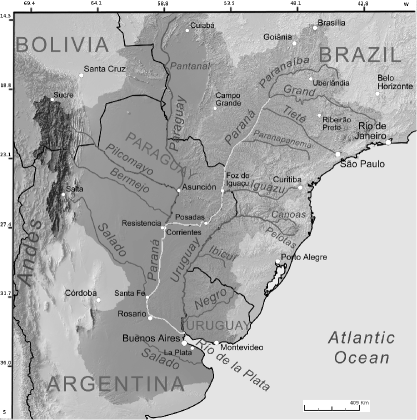
Figure 5: Paraná’s basin. The main rivers of Paraná system are showed. Corrientes city in Argentina is marked. Other South-American cities in Uruguay, Brazil, Bolivia and Paraguay are also indicated.

Significant spectral power between 8.4-9.2 yr was reported by Robertson and Mechoso (1998) and Krepper et al. (2008) for Paraná River. We analysed Paraná River discharge series from Secretaría de Recursos Hídricos of Argentina (http://www.hidricosargentina.gov.ar/acceso_bd.php), we follow Antico and Kröhling (2011) by using the same Corrientes (27^∘28.5^′S, 58^∘50^′W) gauging station data (see Fig. 5). To date (early 2014), there are daily data and monthly averaged data from January 1st, 1904 to August 31th, 2012. For the analysis we starts with monthly data and performed the analysis both using monthly and annual-mean data, the annual data were obtained averaging monthly data for the corresponding year. Therefore, we have taken into account $N=1304$ (for monthly basis analysis) and $N=108$ (annually averaged data). For the annual analysis, we have only taken into account data till 2011 because 2012 datasets are incomplete.

Results from the annual and monthly data sets are comparables. Fig. 6. shows the results for the monthly data. The MEM spectra show prominent peaks at 6.5 yr, 7.6 yr, 8.7 yr and 10.4 yr. It seems that Paraná River has more peaks in this spectral zone than $|T|$ torque of giant planets. Strictly inside the 7-9 yr band only one peak around 7.6 yr is commonly shared between planetary $|T|$ and the river record.

Now, we address the problem of the significance of these peaks, we want to be sure that these peaks are statistically meaningful signals, i.e., that we are not fitting a subtantial amount of noise in the AR model. The MEM spectra can be constrained with red-noise spectra using a Monte Carlo permutation test, as was made by Pardo-Igúzquiza and Rodríguez-Tovar (2005). The MAXEMPER software coming from this publication (http://www.iamg.org/ind ex.php/publisher/articleview/frmArticleID/118) evaluates the statistical significance of the spectral estimates using the mean power spectra of the $N^{\prime}$-th random permutation. This mean spectra is using for testing the null hypothesis from which the spectra of the random permutations are sampled. The outputs include the achieved significance levels of the power spectrum estimated for each frequency. Fig. 7 shows the confidence level of the signal that reaches $95\%$ and higher. Panel a) shows significant power in $\sim$ 7-10.5 yr band for $M=N/4$, panel b) depicts the same for $M=N/3$ and the last one shows the significant spectra for $M=N/2$. We see how the central 7-9 yr band is refined in more detailed spectral lines: in addition, the 6.5 yr line is increasing in importance reaching the $99\%$ confidence level, the 10.4 yr peak is only visible with a (reasonable) value of $M=N/2$, but significant at $95\%$ level against red-noise spectrum.

In order to carry out a even more stringent analysis and eliminates red noise of monthly series, we performed a Singular Spectrum Analysis (SSA) by using the same SSA-MTM-toolkit. We used a conservative $M=130$ spectral window (enough to resolve 6-yr periodicities) with 11 temporal empirical orthogonal functions (T-EOFs); then, we selected those T-EOFs which are oscillatory according to the corresponding test (specificaly, strong FFT). Hence we retain three oscillatory pairs (T-EOFs 1-2, 4-5, 6-7), and performed the reconstruction using the corresponding principal components. Then we used this reconstructed-filtered signal to perform MEM. The result in Fig. 8 yields basically the same spectral peaks as shown in Fig. 6. Therefore we accept that these detected peaks around 6.5 yr, 7.6 yr, 8.7 yr and 10.4 yr, with $M=N/2$, are statistically significant.

This refinement of the MEM spectrum also shows important power above 10-yr periodicities, i.e., around 12-13 yr and 18-19 yr. MAXEMPER permutation test shows that this periods are significant (respectively) at 95$\%$ and $99\%$ confidence level. In Sec. 6, WTC coherence analysis will show that this last spectral zone might play an important role in this problem.

5 The scalar torque modulus, $|T|$, and vectorial torque, ${\bf\Gamma}$, variation

The importance of the vectorial torque ${\bf\Gamma}$ should be addressed and highlighted. So far, torque parameter, $T$, is the only physical quantity cited in this issue, but $T$ is a scalar that only take into account $L$ variations. ${\bf\Gamma}$ = d${\bf L}$/d$t$ is the quantity that measures the total angular momentum variation of the inertial movement of the Sun. Then, let us to analyse the torque strength or vectorial torque modulus $|{\bf\Gamma}|={\it\Gamma}$. Following Eq. 5, we have:

$$|T|={\it\Gamma}\,|{\rm cos}({\bf\Gamma},{\bf L})|$$ (7)

the argument of the cosine function is the angle between ${\bf\Gamma}$ and ${\bf L}$ associated directions. In what follows, accordingly with our findings, we discard the contribution of the terrestrial planets and only consider the influence of the giant planets (i.e, $T_{G}$).

As the planetary movement is quasi-planar, and the solar L vector is basically directed to $z$-axis of the inertial system for long time intervals (see Cionco and Compagnucci, 2012, for a detailed evolution of SBO inclination), we can expect that that cycles in ${\it\Gamma}$ due to giant planets, to be the real origin of these sub-decadal frequencies in $|T_{G}|$. For testing this idea, we calculate the MTM and MEM spectrum of ${\it\Gamma}$. We found that both MTM spectra and the MEM peaks (result not showed for brevity), are coincidental and agrees with $|T_{G}|$ spectra previously obtained in Sec. 3. An analysis of cosine function of Eq. 7, do not show any significant power in the sub-decadal band. Also, a periodogram analysis performed over ${\it\Gamma}$ derived from JPL’s DE431 long-term ephemeris, yields the same peaks reported in Sec. 3. The reason that previously analyses only take $|T|$ into account but do not analyse the vectorial torque in this problem is unknown to us, at least on physical grounds. Analysing the torque modulus the same relationships should have been found and this seems to be more clear and natural.

After confirming that cycles in ${\it\Gamma}$ produces the observed periods in $|T|$ torque, we now return our attention to the directional variations of ${\bf L}$ in space. In addition to that oscillations in ${\bf L}$ modulus, this vector has a precessional-like and nutational-like movements around $z$-axis of the inertial system. We note that the inclination of the SBO has customary variations of few degress ($\sim$ 1-6 deg) (Cionco and Compagnucci, 2012). This kind of “nutation in obliquity”, is certainly of very low amplitude, but the precession-like movement of the SBO orbit is easily seen following the evolution of the ascending node ($\Omega$) of the SBO, this is the same precessional movement of ${\bf L}$ around $z$-axis of the inertial system (because ${\bf L}$ is normal to the orbital plane by definition, and the nodal line is perpendicular to $z$-axis of the inertial system). Fig. 9 shows $\Omega$ variations in the studied period. We can clearly see as $\Omega$ varies between 0 and 360 deg and also performs bounded oscillations, alternatively, through the time. Nevertheles, for simplicity sake, we will refer to this precession-regression movement as a precesional change of ${\bf L}$ around inertial $z$-axis.

At this moment, it is important to note that planetary tidal effects and spin-orbit coupling have been the main lines of inquiry about the underlying physical mechanism in the planetary hypothesis of solar cycle. The giant planets frequencies involved in the sub-decadal band ruled out classical tidal effects in this problem, i.e., tidal effects involving terrestrial planets. As we discussed, the time evolution of ${\bf L}$ is not trivial. The angular momentum vector has basically its most important component along $z$-axis of the inertial system, it has continuous oscillations, precessional-like changes and brief and sporadic rotations of about one year, when solar orbit is gradually inverted (Cionco and Compagnucci, 2012). This means that planetary torque also produces appreciable changes in the direction of angular momentum in the inertial space and also more specifically, with respect to the Sun’s spin axis (${\bf S}$). Authors such as Chang (2009), Javaraiah (2015), Javaraiah (2005) and Juckett (2003) have analysed Sun’s rotation and sunspots distribution showing similar periodicities found in $T$ series (i.e., $\sim$ 8-9 yr). That, has been considered as the evidence of a spin-orbit coupling in the Sun. Perryman and Schulze-Hartung (2011) have taken this mechanisms into consideration and have argued that exoplanetary systems could be a useful environment for further testing and corroboration of a solar spin-orbit coupling hypothesis. These authors have only taken into account variations in spin rate of the Sun’s rotation axis respect to variations in $T$ torque. We have already calculated the frequencies involved in the variation of the modulus of ${\bf\Gamma}$ which, in turn, rules $L$ variations. Now, we are going to evaluate the directional change of ${\bf L}$, but with respect to the Sun’s spin axis, ${\bf S}$.

6 ${\bf L}$ and ${\bf S}$ geometrical relationship

The simplest way to relate ${\bf S}$ and ${\bf L}$ is by studying the orientation of ${\bf L}$ respect to ${\bf S}$ through the time. As far as the author knowledge, this geometrical relationship has not been performed or studied in the literature. Juckett (2000) studied the normalized projection of ${\bf r}$ towards ${\bf S}$, he proposed this geometrical projection (which is basically the $\cos({\bf r},{\bf S}$)) as an “spin-orbit indicator” and searched in this indicator for giant planets signal at over-decadal and longer timescales. Nevertheless, the use of ${\bf r}$, instead of ${\bf L}$, could be inadequated. Although ${\bf r}$ is perpendicular to ${\bf L}$, by definition (then variations in ${\bf r}$ can express variations in ${\bf L}$), ${\bf r}$ evolves with Sun’s orbital motion, independent of ${\bf L}$ position in the inertial space, then, that proposed indicator, has other frequencies not related to the relative evolution between ${\bf L}$ and ${\bf S}$. Moreover, taking into account that ${\bf S}$ is neither fix in the inertial system, the situation is even more complex in reality because it evolves secularly.

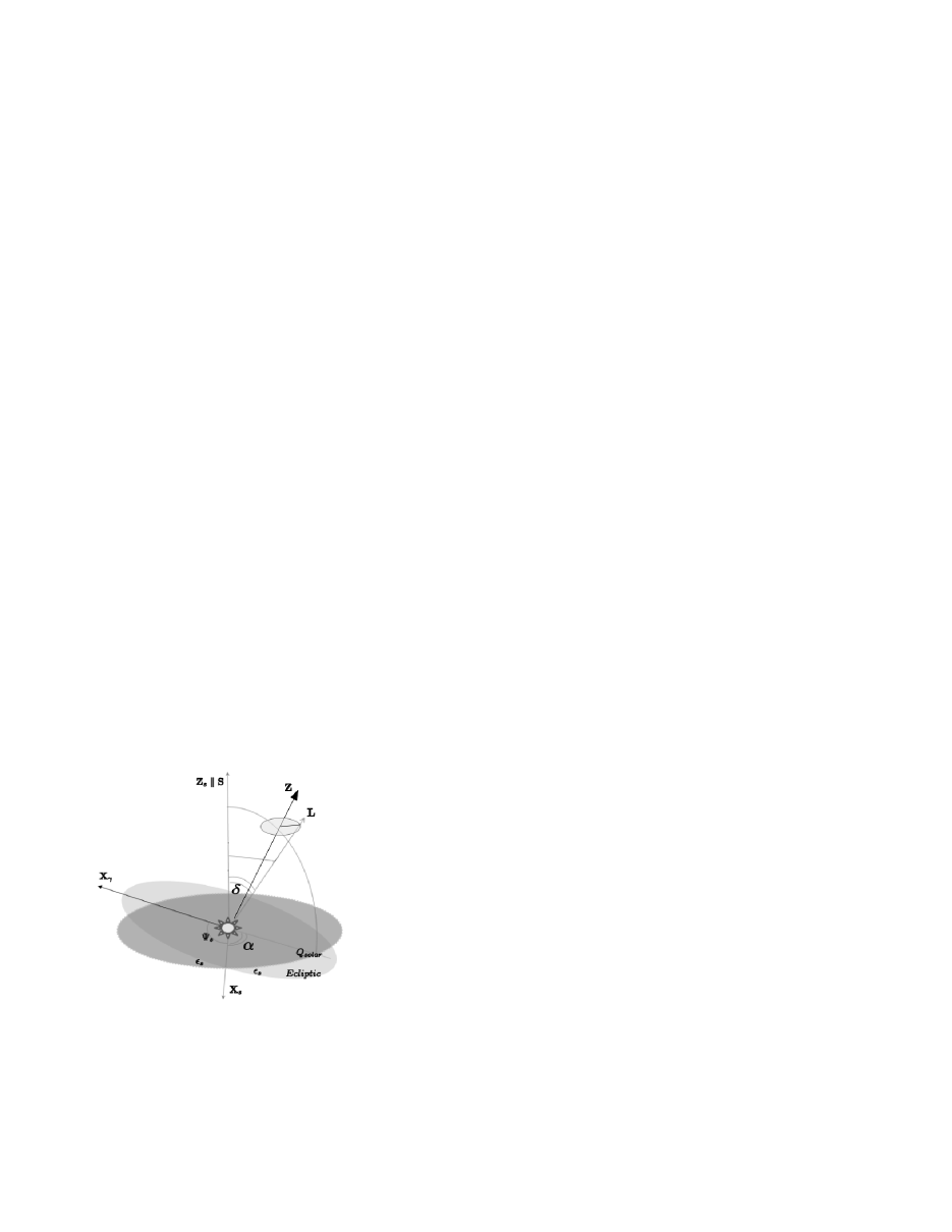
Figure 10: Sketch of the IHS system showing the solar equator ($Qsolar$), the ecliptical plane (the $x$-$y$ plane of the inertial system) and its pole ${\bf Z}$ (the $z$-axis of the inertial system). The angles of orientation $\epsilon_{s}$ and $\Psi_{s}$ between the IHS and the inertial system are indicated (the orientation between ${\bf S}$ and ${\bf Z}$ was largely exagerated by convenience). The ${\bf L}$ vector has a precessional-like movement around $z$-inertial axis (it was idealized by the shadowed ellipse). The position angles of ${\bf L}$ respect to ${\bf S}$ ($\alpha$ and $\delta$) are indicated with double arcs.

To accomplish this LS relationship task, the ecliptical-inertial system will be the linkage between the angular momentum and the Sun associated coordinate system. We adopted the Inertial Heliographic System (IHS) attached (but not fixed) to the Sun (Burlaga, 1984; Fränz and Harper, 2002). In this system the $z$-axis is defined along the Sun’s spin axis and the $x$-$y$ plane coincides with the solar equator. Then, the system is defined with respect to the inertial system by means of the Sun’s obliquity $\epsilon_{S}$, and the longitude $\Psi_{S}$ of the intersection between the ecliptic and the solar equator (Fig. 10). We adopted their values referenced to the epoch J2000.0 (Fränz and Harper, 2002):

$$\epsilon_{S}=7^{\circ}.25$$ (8)

$$\Psi_{S}=75^{\circ}.76+1^{\circ}.397\,(t_{0}-t)$$ (9)

where $t_{0}-t$ is the fraction of Julian century from J2000.0. Then the $x$-axis of the IHS system (${\bf Xs}$) is the intersection of the solar equator and the ecliptic of the corresponding epoch. Therefore, we linked the inertial and the IHS system by means of the following rotation matrix product:

$$(x_{s},y_{s},z_{s})^{t}={\bf R}(\epsilon_{S}){\bf R}(\Psi_{S})(x,y,z)^{t}$$ (10)

$x_{s}$, $y_{s},$ and $z_{s}$ are the components in the IHS system of the $(x,y,z)$ vector in the inertial system.

The positioning of ${\bf L}$ with respect to ${\bf S}$ can be acomplished as usual in spherical astronomy, i.e., using two spherical angles associated with two orthogonal directions on the celestial sphere: $\delta$ measured from the Sun’s spin axis toward ${\bf L}$ (a kind of colatitude angle), and $\alpha$, measured from ${\bf X_{S}}$ towards the arc of great circle that connect ${\bf S}$ and ${\bf L}$ (a longitudinal angle; see Fig. 10). Both angles are defined by the following expressions:

$${\rm cos}(\delta)=\frac{Lz_{s}}{L}$$ (11)

$${\rm cos}(\alpha)=Lx_{s}\,[L^{2}-Lz^{2}_{s}]^{-1/2}$$ (12)

where $Lz_{s}$ and $Lx_{s}$ are the $z$ and $x$-component of ${\bf L}$ in IHS. Then, we follow the evolution of ${\bf L}$ respect to ${\bf S}$ for the same period consistently with Paraná River data. We analysed from 1904-2012 A.D., and then performed spectral analysis to both positional angles. Fig. 11 show the evolution of $\alpha$ and $\delta$. The co-latitudinal angle $\delta$ shows very small amplitude oscillations but a sudden increase around 1990 because of the above-mentioned orbital invertion (${\bf L}$ invertion). The longitudinal angle $\alpha$ shows more important oscillations of about 20 deg in amplitude, with marked peaks each $\sim 38$ yr, (which are also visible, but lesser pronounced, in $\delta$). These secondary peaks occur at Jupiter, Saturn and Neptune alignments (remember that the recorded mean S-N period is $\sim$ 36 yr). The exceptional four giant planets alignment of 1990 is also seen.

Consequently, MEM and MTM analyses of $\delta$ do not show any significant spectrum (results not shown here), but $\alpha$ evolution shows very significant spectral power in the sub-decadal band. This spectrum is showed in Fig. 12, where Paraná MTM spectrum is also depicted for comparison. In this figure, we have plotted two vertical lines delimiting the spectral zone in wich the power of $D$ is larger than $50\%$ red noise significance level. Interestingly, we note that the Paraná spectrum is much more similar to $\alpha$ spectrum than the $|T|$ (or $|T_{G}|$) spectrum at sub-decadal band (compare with Fig. 1). Indeed, MEM spectrum of $\alpha$ shows significant peaks, coincidents with Paraná River periodicities (Fig. 13). We can see four significant peaks at 6.3 yr, 7.7 yr, 8.6 yr and 9.9 yr. Respect to $|T_{G}|$ spectra, these periodicities are certainly the same as Fig. 4, with the addition of a peak in 8.6 yr. Using the same methodology applied in Sec. 3 to identify the peaks in $|T_{G}|$ signal, we conclude that these peaks are due only to Jupiter, Saturn and Neptune, and this peak at 8.6 yr also comes from the mixing of these planets’ periods in the formula (12).

Two peaks of 7.7 yr and 8.6 yr practically coincides with Paraná peaks inside 7-9 band (7.6 yr and 8.7 yr). Particularly, this 8.6-yr period is very close to the Po and Paraná Rivers strongest peak. The percentage difference between Paraná River’s spectral peaks and $\alpha$ periodicities in the sub-decadal band is lesser than $5\%$. At this point, it is interesting to note that, taking into account the Nyquist theorem, the approximate error in the determination of periods ($p$) in Paraná River’s series ($L=108$ yr) is $\sim p^{2}/(2L)$ (Tan and Cheng, 2013); then, the 10.4-yr peak is ranging from 9.9 yr to 10.9 yr; i.e, $\sim 5\%$ of error. Then, in the context of the previous related (empirical) studies, we have found a stronger phenomenology; and this, can be linked to a physical hypothesis of Sun-planets interaction, i.e., a putative solar spin-orbit coupling effect depending on this LS geometry. Now, we are going to evaluate if these $\alpha$ and $D$ signals have any degree of spectral coherence as to take into consideration our proposed LS relationship in a plausible scenario of Sun-rivers physical relationship.

7 $\alpha$ and $D$ spectral coherence analysis

Fortunately, we have several methods to evaluate the frecuency-domain similarity or spectral coherence between two signals. The coherence function or MSC can be evaluated by several methods (see e.g. Benesty et al., 2006; Holm, 2014a; Scafetta, 2014). After several initial trials with synthetic signals, we have decided to use the Minimum Variance Distortionless Response (MVDR) (Benesty et al., 2006) for evaluating MSC because it is more accurate (or restrictive) in the isolation of the significant frequencies than the usual routines based on Welch’s periodogram method. We used the Matlab MVDR implementation of Benesty et al. (2006) (http://www.mathworks.com /matlabcen tral/fileexchange/9781-coherence-function/content/cohe rence_MVDR). MVDR is also easier to use: it only depends on the number of filters ($K$) and their window lenght ($L$). To get better resolution than annually data, we have analysed both $\alpha$ and $D$ data on monthly basis ($N=1304$) and used $L=108$ yr (see e.g. Benesty et al., 2006; Scafetta, 2014). Tha planetary data was simulated taking 12 values per year of 365.25 yr; no averaging was performed on it. The data sets were detrended and $z$-standarized.

For evaluating the MSC coherence between $\alpha$ and $D$ signals and its confidence levels, we found the MVDR coherence of the original signals and also performed a Monte Carlo permutation test in the strategy of Pardo-Igúzquiza and Rodríguez-Tovar (2005), i.e., finding the Achieved Significance Level for each sampled frequency. It is the probability to get, by chance, a surrogate MSC signal grater than the original MSC signal. We performed 5000 permutations with no restrictions, so a stringent withe noise hypothesis have been used. Finally, it is straightforward to obtain de Achieved Confidence Level (ACL) for each frequency-periodicity. Fig 14 shows this: the solid line is the ACL of the MSC calculation obtained in the Monte Carlo test. The dashed line is the 95% confidence level. Therefore, MSC between $\alpha$ and $D$ signals, are statistically significant at 95% confidence level around 8-yr periodicity. This is an encouraging result, despite its marginal significance. This could indicate intermittent coherence along the time.

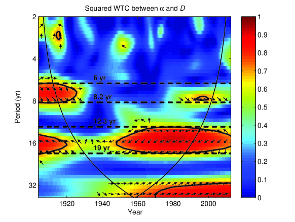
Figure 15: Squared WTC coherence between $D$ and $\alpha$ series. It confirms the coherence’s intermittency around 8-yr band. The horizontal dashed lines are the approximated bounds of 95$\%$ confidence level zones, they marks periodicities between 6-8.2 yr and 12.3-19 yr.

To study this, we used an independent method based on Wavelet Transform (squared WTC, Grinsted et al., 2004). We used the corresponding software at http://noc.ac.uk/using-science/crosswavelet-wavelet-coher ence. The result is showed in Fig. 15. WTC detects high level of coherence between 6-8.2 yr. This coherence seems to be stable until 1930, then later return about 1990, but specifically around 8-yr periodicity. These signals seems to be out of phase ($\sim-45$ deg) with some tendency to be in-phase. Another more important island of coherence appears inside 12-19 yr band (specifically between 12.3-19 yr), where the signals are out-of-phase/anti-phase. This spectral zone is very signifcant for $\alpha$ signal, it is related to Jupiter orbital period, J-S, J-N, S-N/2, etc. Spectral power around 13 yr and 18 yr was also observed in the SSA filtered MEM analysis (Fig. 8), and confirmed by Monte Carlo permutation test. Therefore, squared WTC appears also to detect very significant coherence at this over-decadal spectral band.

8 Discussion and concluding remarks

In this effort, we have re-evaluated key dynamical aspects related to the evidence presented in the past linking solar inertial motion and discharges from Po and Paraná Rivers. We have explained the cycles and the physical origin of the signals present in the oscillations of $|T|$, the most important parameter taken into account in these empirical evidences. We showed the existence of three clear frequencies, originated in the variations of the vectorial torque modulus (${\it\Gamma}$) ruled by the planets Jupiter, Saturn and Neptune. We also improved prior results on Paraná River discharge periodicities, showing the existence of four significan spectral peaks.

Since the detected importance of vectorial torque in this problem, we found basically the same Paraná discharge spectral peaks in the spectrum of the longitudinal variations ($\alpha$ angle variations) of ${\bf L}$ with respect to ${\bf S}$ (which are ruled by the same set of planets). Having ruled out the tidal hypothesis in this problem, this result stresses the importance of the vectorial torque, taking into account the hypothesis of a possible solar spin-orbit coupling effect. In addition, Po River also shows a sub-decadal spectral peak (8.2-8.7 yr) more similar to $\alpha$ spectrum peaks than $|T|$ spectrum peaks.

Beyond these spectral matches and phenomenologycal coincidences, we were able to obtain significant mathematical coherence between both $\alpha$ and $D$ signals, which is a very encouraging result. These findings suggest that, if these rivers are trully linked to solar dynamics, the physical origin of this connection might be related to a working solar spin-orbit interaction. Nevertheless, to describe the complete scenario, we must seek for a terrestrial linkage between Sun-planets interactions and river dynamics. This “atmospheric driver” would be the directly responsible for perturbing river dynamics, whereas it respond to external, solar fluctuations. This putative driver, should show a very good coherence with both Sun dynamics and river dynamics at particular spectral bands; but certainly, it would act as a filter, enhancing particular cycles and attenuating others, following its own dynamics, which can also produce different responses in different rivers, taking into account their locations on the Earth.

The North Atlantic Oscillation (NAO), was proposed as a driver of this possible Sun-rivers connection. Zanchettin et al. (2008) have showed that NAO is correlated with both solar activity and Po River discharge at sub-decadal time-scale. Scafetta (2010) suggests a NAO and solar inertial motion relationship at multi-decadal timescale. Oscillatory modes between 7-8 yr have been detected by Paluš and Novotná (2009) in NAO and geomagnetic index. Also, Georgieva et al. (2012) have shown strong connection among heliospheric activity, geomagnetism and NAO oscilations. Therefore, changes in solar magnetic activity, NAO oscillations and variations of hydrological patterns related to Po River, are spected to be strongly connected.

By other hand, Robertson and Mechoso (1998) have related at sub-decadal time-scale, anomalous cool events in Tropical North Atlantic (TNA) with high South-America rivers runoff. This seems to have motivated Antico and Kröhling (2011) to propose a possible relationship NAO-Paraná. A more difficult issue to address is the influence that NAO (as a whole atmospheric-oscillatory system) might have over South-America, at this sub-decadal time-scales. The TNA affects intertropical South-America via, e.g., decadal variability of the summer monsoon system (Robertson and Mechoso, 1998); then, it is possible that TNA acts as agency between South-American precipitation regime and NAO.

Paraná’s basin presents very inhomogeneous regions with different hydrological patterns. The average annual precipitation decreases from east to west (i.e., as we move away from the Atlantic Ocean), but also from north to south (de Petris and Paquini, 2007). Pinto Neto et al. (2013) have recently showed that thunderstorm days in Brazil are correlated to solar activity; but a very specially feature arise from their work: the most southern data set used, coming from Porto Alegre city station, shows a broad spectral peak around 8 yr. They related their findings to possible magnetic activity changes in Earth atmosphere. Porto Alegre city is almost at the same latitude than Corrientes gauging station (Fig. 5). Therefore, it is imperative to study the rainfall regime in other cities of the Paraná basin, looking for these sub-decadal periodicities, and particularilly, a possible north-south gradient with these periodicities (taking into account Pinto Neto et al., 2013, results).

South-east of Brasil is the centre of the South Atlantic Magnetic Anomaly (SAMA). It produces the sinking of charged particles trapped in atmospheric belts (Pinto et al., 1992). This anomaly (unique phenomenon in the world) affects almost all Paraná basin, but is stronger at the south-east of the basin. Therefore, solar, geomagnetic and atmospheric activity should be carefully investigated, as a whole, in this region. We think that Sun-climate relationship with magnetic activity variations, should be considered as the potential connection of these possible Sun-river relationships. Sub-decadal variations of charged particles coming from the Sun (for instance, driven by a solar spin-orbit interaction), could interact with Earth atmosphere and geomagnetism, producing complex climatic patterns.

Earth climate variations with relation to a possible solar spin-orbit coupling have also been argued by Shirley (2009), taking into account solar meridional fluxes changing velocities. Geomagnetic activity is strongly dependent on solar dynamo, through changes or alternations in poloidal and toroidal fields (e.g., Georgieva et al., 2012), then a possible relationship between heliospheric parameters and the Earth atmosphere, and this as a trigger of hydrometeorological signals, is expected. A spin-orbit coupling hypothesis was called upon to explain some phenomenological concordances between $L$ variations and solar activity, through solar rotation and functioning of a magnetohydrodynamical dynamo. The original idea seems to be first proposed by Jane Blizard (1981), and has since been taken into consideration also by Javaraiah (2005), Juckett (2003, 2000), Perryman and Schulze-Hartung (2011), Shirley (2006), Shirley (2014), Zaqarashvili (1997). The idea is that planets can transfer orbital momentum to the Sun’s rotational angular momentum, and this variation could interact with the solar dynamo through a putative mechanism. Therefore, some part of the orbital angular momentum could be transferred to spin angular momentum. The inverse can also be true as was shown by Javaraiah (2005). As was mentioned Javaraiah (2005) and Juckett (2003) show evidence that certain periods in Sun’s rotation are very similar to periods in $T$ power spectrum, especially the 8-yr periodicity. Here, we have presented a complementary side of this possible physical phenomena, i.e., the study of the directional variations between ${\bf L}$ and ${\bf S}$. It is also interesting to note that, oscillations of $\sim 8.5$ yr have also been measured in solar cycle (Rozelot, 1994). Periods from 6-8 yr has been found in drifts of latitudinal bands of near-equal rotational velocity in the Sun (Makarov et al., 1997).

At present, there is still no clear physical mechanism to explain how this transference of angular momentum might be achieved. In planetary dynamics, spin-orbit coupling refers to spin-orbit resonance (see e.g. Murray and Dermott, 1999, Chap. 5 for this subject), i.e., a commensurability that appear between the spin rate of a body and its orbital period. In general, the spin axis of the body is considered parallel to its orbital angular momentum vector (spin perpendicular to the orbit or zero obliquity approximation). The mechanism behind this coupling is the tidal friction originated by a planet over a satellite (Goldreich and Soter, 1966), or by the Sun to the planets (Goldreich and Peale, 1966; Peale and Gold, 1965). Goldreich and Soter (1966), argue that tides raised on the Sun by planets have virtually no effect on the rotation and orbit of the Sun. But this does not preclude the fact that certain internal solar dynamics can be susceptible to external gravitational modulation and perturbation (Scafetta, 2012a,b; Wolff and Patrone, 2010). Our problem at hand is more complex, because the solar orbital angular momentum has great variations (in modulus and direction), unlike of the orbital angular momentum variations of the planets. A model of solar spin-orbit coupling was out of the scope of this work; we only arrived at a spin-orbit relationship following the dynamics involved in this problem. But we can say that any model of solar spin-orbit interaction should consider (see e.g. Peale, 2005): a) an adequate expansion of the gravitational potential of the Sun that accounts for the Sun’s permanent figure, and the calculation of the corresponding planetary torque; b) the tidal torque of the planets and; c) the frictional torque coming from different solar internal zones (tachocline, convective envelope, etc). These zones have different shapes/forms (e.g., ellipticities) and then, they could precesses at different rates (Poincaré, 1910). Therefore, these ingredients are essential to a detailed description of the Sun’s spin axis evolution (tilt and rate) and its possible coupling with the orbital angular momentum at different time-scales. Our findings also suggest that, at least, we must consider the contributions of planets Jupiter, Saturn and Neptune. For example, Chang et al. (2012), recently shown how a young star can modify its axial tilt by the magnetic torque that arises from the Ohmic dissipation in a Hot-Jupiter planet system, at the expense of the spin-orbit energy (see Eq. 17 of that paper for a spin-orbit coupling expression). The idea of Abreu et al. (2012) about the planetary tidal interaction in the tachocline, which has been modelled as an ellipsoidal figure, is a good candidate for spin-orbit coupling interaction, and should further be studied in this context.

Of course, a lot of work is needed to study several aspects of these processes and hypotheses; specially, to analyse another rivers and the suspected atmospheric drivers. We are working on this, and the results will be the subject of another paper.

FIGURE CAPTIONS (ALL FIGURES IN BLACK-WHITE)

Fig. 1. MTM spectra comparison of Paraná $D$ series and planetary $|T|$ torque. The vertical doted lines mark the common 7-9 yr band considered by Antico and Kröhling (2011). Inside this band, the spectral power of $D$ is significant at 50-95$\%$. The simple inspection of this figure shows that $D$ signal is significant at this levels in a broader sub-decadal band.

Fig. 2. Planetary $T$ torque from 1900 to 2013 A.D. Dashed line: all the planets included; solid line: only giant planets. Physical units: solar mass (Ms), astronomical unity (AU) and days (d).

Fig. 3. Comparison between $T$ torque of only giant planets ($T_{G}$), $T$ from Jupiter and Saturn ($T_{JS}$), and from Jupiter, Saturn and Neptune ($T_{JSN}$) subsystem planets. Surpraisingly, the rapid variation (lesser than 1 yr) in $T$ signal around 1990 is due only to giant planets. The quasi-conjunction of Jupiter with other Giants forces to $T$ to be near zero. The $T$ “perturbation”around 1935 is due to the normal dynamics that strongly involve Neptune planet.

Fig. 4. Maximum entropy (MEM) spectra for $|T_{G}|$ with differents number of poles $(M$) used.

Fig. 5. Paraná’s basin. The main rivers of Paraná system are showed. Corrientes city in Argentina is marked. Other South-American cities in Uruguay, Brazil, Bolivia and Paraguay are also indicated.

Fig. 6. MTM and MEM Spectra of Paraná’s monthly $D$ series (1304 data values used).

Fig. 7. Results of the Monte Carlo permutation test (MAXEMPER software) performed to Paraná monthly $D$ series, showing the significance of these peaks against red noise null hypothesis. The pole order $M$ is showed (number of data $N$= 1304).

Fig. 8. MEM spectrum of the filtered $D$ monthly series showing the disappearance of noisy-peaks ($M=N/2$). The small window shows in detail that the same four peaks appear in the sub-decadal band. For comparison, the arrows indicate the peaks of the raw-annual data.

Fig. 9. Ascending node evolution of the solar barycentric orbit (one point per year), the same oscillations are performed by $\bf{L}$ vector around the $z$-axis of the inertial system, in this case, the ecliptical J2000.0 system.

Fig. 10. Sketch of the IHS system showing the solar equator ($Qsolar$), the ecliptical plane (the $x$-$y$ plane of the inertial system) and its pole ${\bf Z}$ (the $z$-axis of the inertial system). The angles of orientation $\epsilon_{s}$ and $\Psi_{s}$ between the IHS and the inertial system are indicated (the orientation between ${\bf S}$ and ${\bf Z}$ was largely exagerated by convenience). The ${\bf L}$ vector has a precessional-like movement around $z$-inertial axis (it was idealized by the shadowed ellipse). The position angles of ${\bf L}$ respect to ${\bf S}$ ($\alpha$ and $\delta$) are indicated with double arcs.

Fig. 11. $\alpha$ and $\delta$ evolution in the studied period. The most important peaks occur each $\sim$ 38 yr, due to Jupiter, Saturn and Neptune alignments. The greatest peak around 1990 involve the four giant planets.

Fig. 12. MTM spectra of Paraná and $\alpha$ series. The vertical lines mark the band at which the spectral power of $D$ is significant at 50-95$\%$. Surprisingly, in this sub-decadal band four peaks seem to be very similar in both series. Certainly, Paraná spectrum is more similar to $\alpha$ spectrum than $|T_{G}|$ spectrum. Also, a prominent bi-decadal band is also seen in $\alpha$ spectrum.

Fig. 13. MEM spectra of Paraná $D$ series and $\alpha$ series. It confirms the existence of four peaks. Therefore in the sub-decadal band Paraná’s $D$ series has virtually the same frequencies than $\alpha$ series (the porcentual error is lesser than 5$\%$).

Fig. 14. Achieved Confidence Level (ACL) of the MSC (MVDR method), with Monte Carlo permutation test, between Paraná $D$ series and $\alpha$ series. Periodicities around 8 yr are statistically significant at 95$\%$ confidence level.

Fig. 15. Squared WTC coherence between $D$ and $\alpha$ series. It confirms the coherence’s intermittency around 8-yr band. The horizontal dashed lines are the approximated bounds of 95$\%$ confidence level zones, they marks periodicities between 6-8.2 yr and 12.3-19 yr.

Figure 1: MTM spectra comparison of Paraná $D$ series and planetary $|T|$ torque. The vertical doted lines mark the common 7-9 yr band considered by Antico and Kröhling (2011). Inside this band, the spectral power of $D$ is significant at 50-95$\%$. The simple inspection of this figure shows that $D$ signal is significant at this levels in a broader sub-decadal band.

Figure 2: Planetary $T$ torque from 1900 to 2013 A.D. Dashed line: all the planets included; solid line: only giant planets. Physical units: solar mass (Ms), astronomical unity (AU) and days (d).

Figure 3: Comparison between $T$ torque of only giant planets ($T_{G}$), $T$ from Jupiter and Saturn ($T_{JS}$), and from Jupiter, Saturn and Neptune ($T_{JSN}$) subsystem planets. Surpraisingly, the rapid variation (lesser than 1 yr) in $T$ signal around 1990 is due only to giant planets. The quasi-conjunction of Jupiter with other Giants forces to $T$ to be near zero. The $T$ “perturbation” around 1935 is due to the normal dynamics that strongly involve Neptune planet.

Figure 4: Maximum entropy (MEM) spectra for $|T_{G}|$ with differents number of poles $(M$) used.

Figure 6: MTM and MEM Spectra of Paraná’s monthly $D$ series (1304 data values used).

Figure 7: Results of the Monte Carlo permutation test (MAXEMPER software) performed to Paraná monthly $D$ series, showing the significance of these peaks against red noise null hypothesis. The pole order $M$ is showed (number of data $N$= 1304).

Figure 8: MEM spectrum of the filtered $D$ monthly series showing the disappearance of noisy-peaks ($M=N/2$). The small window shows in detail that the same four peaks appear in the sub-decadal band. For comparison, the arrows indicate the peaks of the raw-annual data.

Figure 9: Ascending node evolution of the solar barycentric orbit (one point per year), the same oscillations are performed by $\bf{L}$ vector around the $z$-axis of the inertial system, in this case, the ecliptical J2000.0 system.

Figure 11: $\alpha$ and $\delta$ evolution in the studied period. The most important peaks occur each $\sim$ 38 yr, due to Jupiter, Saturn and Neptune alignments. The greatest peak around 1990 involve the four giant planets.

Figure 12: MTM spectra of Paraná and $\alpha$ series. The vertical lines mark the band at which the spectral power of $D$ is significant at 50-95$\%$. Surprisingly, in this sub-decadal band four peaks seem to be very similar in both series. Certainly, Paraná spectrum is more similar to $\alpha$ spectrum than $|T_{G}|$ spectrum. Also, a prominent bi-decadal band is also seen in $\alpha$ spectrum.

Figure 13: MEM spectra of Paraná $D$ series and $\alpha$ series. It confirms the coincidence between four peaks. Therefore in the sub-decadal band Paraná’s $D$ series has virtually the same frequencies than $\alpha$ series (the porcentual error is lesser than 5$\%$).

Figure 14: Achieved Confidence Level (ACL) of the MSC (MVDR method), with Monte Carlo permutation test, between Paraná $D$ series and $\alpha$ series. Periodicities around 8 yr are statistically significant at 95$\%$ confidence level.

References

- Abreu et al. (2012) Abreu, J. A., Beer, J., Ferriz-Mas, A., McCracken, K. G., Steinhilber, F. 2012. Is there a planetary influence on solar activity? Astronomy and Astrophysics 548, A88.
- Agnihotri et al. (2011) Agnihotri, R., Dutta, K., Soon, W. 2011. Temporal derivative of Total Solar Irradiance and anomalous Indian summer monsoon: An empirical evidence for a Sun-climate connection. Journal of Atmospheric and Solar-Terrestrial Physics 73, 1980-1987.
- Antico and Kröhling (2011) Antico, A., Kröhling, D. M. 2011. Solar motion and discharge of Paraná River, South America: Evidence for a link. Geophysical Research Letters 38, 19401.
- Benesty et al. (2006) Benesty, J., Chen, J., Huang, Y. 2006. Estimation of the coherence function with the MVDR approach. Acoustics, Speech and Signal Processing. ICASSP 2006 Proceedings 3, 500-503. doi: 10.1109/ICASSP.2006.1660700.
- Blizard (1981) Blizard, J. B. 1981. Solar Motion and Solar Activity. Bulletin of the American Astronomical Society 13, 876.
- Brown (1900) Brown, E. W. 1900. A possible explanation of the sun-spot period. Monthly Notices of the Royal Astronomical Society 60, 599.
- Burlaga (1984) Burlaga, L. F. 1984. MHD processes in the outer heliosphere. Space Science Reviews 39, 255-316.
- Cameron and Schüssler (2013) Cameron, R. H., Schüssler, M. 2013. No evidence for planetary influence on solar activity. Astronomy and Astrophysics 557, A83.
- Cionco and Compagnucci (2012) Cionco, R. G., Compagnucci, R. H. 2012. Dynamical characterization of the last prolonged solar minima. Advances in Space Research 50, 1434-1444.
- Chambers (1999) Chambers, J. E. 1999. A hybrid symplectic integrator that permits close encounters between massive bodies. Monthly Notices of the Royal Astronomical Society 304, 793-799.
- Chang et al. (2012) Chang, Y.-L., Bodenheimer, P. H., Gu, P.-G. 2012. Coupled Evolutions of the Stellar Obliquity, Orbital Distance, and Planet’s Radius due to the Ohmic Dissipation Induced in a Diamagnetic Hot Jupiter around a Magnetic T Tauri Star. The Astrophysical Journal 757, 118.
- Charvátová (2009) Charvátová, I. 2009. Long-term predictive assessments of solar and geomagnetic activities made on the basis of the close similarity between the solar inertial motions in the intervals 1840 1905 and 1980 2045. New Astronomy 14, 25-30.
- Charvátová and Střeštík (2004) Charvátová, I., Střeštík, J. 2004. Periodicities between 6 and 16 years in surface air temperature in possible relation to solar inertial motion. Journal of Atmospheric and Solar-Terrestrial Physics 66, 219-227.
- Chang (2009) Chang, H.-Y. 2009, Periodicity of North South asymmetry of sunspot area revisited: Cepstrum analysis, New Astronomy, 14, 133-138.
- Cubasch et al. (2006) Cubasch, U., Zorita, E., Kaspar, F., Gonzalez-Rouco, J. F., von Storch, H., Prömmel, K. 2006. Simulation of the role of solar and orbital forcing on climate. Advances in Space Research 37, 1629-1634.
- de Petris and Paquini (2007) Depetris P.J. y Pasquini A.I. 2007. The Geochemistry of the Paraná River: An Overview. In M.H. Iriondo, J.C. Paggi, y M.J. Parma (Eds.). The Middle Paraná River: Limnology of a Subtropical Wetland. Springer-Verlag Berlin Heidelberg.
- Fairbridge and Shirley (1987) Fairbridge, R. W., Shirley, J. H. 1987. Prolonged minima and the 179-yr cycle of the solar inertial motion. Solar Physics 110, 191-210.
- Folkner et al. (2014) Folkner, W. M., Williams, J. G., Boggs, D. H., Park, R. S., Kuchynka, P. 2014, The Planetary and Lunar Ephemerides DE430 and DE431, Interplanetary Network Progress Report, 196, 1.
- Fränz and Harper (2002) Fränz, M., Harper, D. 2002. Heliospheric coordinate systems. Planetary and Space Science 50, 217-233.
- Georgieva et al. (2012) Georgieva, K., Kirov, B., Koucká Knížová, P., Mošna, Z., Kouba, D., Asenovska, Y. 2012. Solar influences on atmospheric circulation. Journal of Atmospheric and Solar-Terrestrial Physics 90, 15-25.
- Ghil et al. (2002) Ghil, M., and 10 colleagues 2002. Advanced Spectral Methods for Climatic Time Series. Reviews of Geophysics 40, 1003.
- Goldreich and Peale (1966) Goldreich, P., Peale, S. 1966. Spin-orbit coupling in the solar system. The Astronomical Journal 71, 425.
- Goldreich and Soter (1966) Goldreich, P., Soter, S. 1966. Q in the Solar System. Icarus 5, 375-389.
- Gray et al. (2010) Gray, L. J., and 14 colleagues 2010. Solar Influences on Climate. Reviews of Geophysics 48, 1-53.
- Grinsted et al. (2004) Grinsted, A., Moore, J. C., Jevrejeva, S. 2004, Application of the cross wavelet transform and wavelet coherence to geophysical time series, Nonlinear Processes in Geophysics, 11, 561-566.
- Holm (2014a) Holm, S. 2014a, On the alleged coherence between the global temperature and the sun’s movement, Journal of Atmospheric and Solar-Terrestrial Physics, 110, 23-27.
- Holm (2014b) Holm, S. 2014b, Corrigendum to “On the alleged coherence between the global temperature and the sun’s movement”;, Journal of Atmospheric and Solar-Terrestrial Physics, 119, 230-231
- Humphreys (1910) Humphreys, W. J. 1910. Solar Disturbances and Terrestrial Temperatures. The Astrophysical Journal 32, 97-111.
- Hung (2007) Hung C.-C., 2007. Apparent Relations Between Solar Activity and Solar Tides Caused by the Planets. NASA Technical Memorandum TM 2007-214817.
- IPCC (2007) IPCC: Climate Change 2007: The Physical Science Basis. Contribution of Working Group I to the Fourth Assessment Report of the Intergovernmental Panel on Climate Change [Solomon, S., D. Qin, M. Manning, Z. Chen, M. Marquis, K.B. Averyt, M.Tignor and H.L. Miller (eds.)]. Cambridge University Press, Cambridge, United Kingdom and New York, NY, USA.
- Javaraiah (2015) Javaraiah, J. 2015, Long-term variations in the north-south asymmetry of solar activity and solar cycle prediction, III: Prediction for the amplitude of solar cycle 25, New Astronomy, 34, 54-64.
- Javaraiah (2005) Javaraiah, J. 2005. Sun’s retrograde motion and violation of even-odd cycle rule in sunspot activity. Monthly Notices of the Royal Astronomical Society 362, 1311-1318.
- Jones et al. (2012) Jones, G. S., Lockwood, M., Stott, P. A. 2012. What influence will future solar activity changes over the 21st century have on projected global near-surface temperature changes? Journal of Geophysical Research (Atmospheres) 117, D05103, 1-13.
- Jose (1965) Jose, P. D. 1965. Sun’s motion and sunspots. The Astronomical Journal 70, 193.
- Juckett (2003) Juckett, D. A. 2003. Temporal variations of low-order spherical harmonic representations of sunspot group patterns: Evidence for solar spin-orbit coupling. Astronomy and Astrophysics 399, 731-741.
- Juckett (2000) Juckett, D. A. 2000. Solar activity cycles, north/south asymmetries, and differential rotation associated with solar spin-orbit variations. Solar Physics 191, 201-226.
- Krepper et al. (2008) Krepper, C. M., García N., Jones P. 2008 Low‐frequency response of the upper Paraná basin, Int. J. Climatol. 28, 351–360.
- Landscheidt (2000) Landscheidt, T. 2000. River Po discharges and cycles of solar activity. Hydrol. Sci. J. 45(3), 491–493
- Landscheidt (1999) Landscheidt, T. 1999. Extrema in sunspot cycle linked to Sun’s motion.. Solar Physics 189, 415-426.
- Landscheidt (1987) Landscheidt, T. 1987. Cyclic distribution of energetic X-ray flares. Solar Physics 107, 195-199.
- Leal-Silva and Velasco Herrera (2012) Leal-Silva, M. C., Velasco Herrera, V. M. 2012. Solar forcing on the ice winter severity index in the western Baltic region. Journal of Atmospheric and Solar-Terrestrial Physics 89, 98-109.
- Makarov et al. (1997) Makarov, V. I., Tlatov, A. G., Callebaut, D. K. 1997. Long-Term Variations of the Torsional Oscillations of the Sun. Solar Physics 170, 373-388.
- Mokhov and Smirnov (2006) Mokhov, I. I., Smirnov, D. A. 2006. El Niño-Southern Oscillation drives North Atlantic Oscillation as revealed with nonlinear techniques from climatic indices. Geophysical Research Letters 33, 3708.
- Murray and Dermott (1999) Murray, C. D., Dermott, S. F. 1999. Solar system dynamics. Solar system dynamics by Murray, C. D., 1999 .
- Okal and Anderson (1975) Okal, E., Anderson, D. L. 1975. On the planetary theory of sunspots. Nature 253, 511-513.
- Paluš and Novotná (2009) Paluš, M., Novotná, D. 2009. Phase-coherent oscillatory modes in solar and geomagnetic activity and climate variability. Journal of Atmospheric and Solar-Terrestrial Physics 71, 923-930.
- Pardo-Igúzquiza and Rodríguez-Tovar (2005) Pardo-Igúzquiza, E., Rodríguez-Tovar, F. J. 2005. MAXENPER: a program for maximum entropy spectral estimation with assessment of statistical significance by the permutation test. Computers and Geosciences 31, 555-567.
- Peale (2005) Peale, S. J. 2005. The free precession and libration of Mercury. Icarus 178, 4-18.
- Peale and Gold (1965) Peale, S. J., Gold, T. 1965. Rotation of the Planet Mercury. Nature 206, 1240-1241.
- Penland et al. (1991) Penland, C., Ghil, M., Weickmann, K. M. 1991. Adaptive filtering and maximum entropy spectra with application to changes in atmospheric angular momentum. Journal of Geophysical Research 96, 22659-22671.
- Perryman and Schulze-Hartung (2011) Perryman, M. A. C., Schulze-Hartung, T. 2011. The barycentric motion of exoplanet host stars. Tests of solar spin-orbit coupling. Astronomy and Astrophysics 525, A65.
- Pinto et al. (1992) Pinto, O., Jr., Gonzalez, W. D., Pinto, I. R. C., Gonzalez, A. L. C., Mendes, O., Jr. 1992. The South Atlantic Magnetic Anomaly - Three decades of research. Journal of Atmospheric and Terrestrial Physics 54, 1129-1134.
- Pinto Neto et al. (2013) Pinto Neto, O., Pinto, I. R. C. A., Pinto, O. 2013. The relationship between thunderstorm and solar activity for Brazil from 1951 to 2009. Journal of Atmospheric and Solar-Terrestrial Physics 98, 12-21.
- Poincaré (1910) Poincaré, H. 1910. Sur la précession des corps déformables. Bulletin Astronomique, Serie I 27, 321-356.
- Poulianovsky and Usoskin (2014) Poluianov, S., Usoskin, I. 2014, Critical Analysis of a Hypothesis of the Planetary Tidal Influence on Solar Activity, Solar Physics, 289, 2333-2342.
- Press et al. (1992) Press, W. H., Teukolsky, S. A., Vetterling, W. T., Flannery, B. P. 1992. Numerical recipes in FORTRAN. The art of scientific computing. Cambridge: University Press, —c1992, 2nd ed.
- Robertson and Mechoso (1998) Robertson, A. W., Mechoso C. R. 1998, Interannual and decadal cycles in river flows of southeastern South America, J. Clim., 11, 2570–2581.
- Rozelot (1994) Rozelot, J. P. 1994. On the stability of the 11-year solar cycle period (and a few others). Solar Physics 149, 149-154.
- Scafetta (2014) Scafetta, N. 2014, Discussion on the spectral coherence between planetary, solar and climate oscillations: a reply to some critiques, Astrophysics and Space Science, in press, DOI: 10.1007/s10509-014-2111-8.
- Scafetta (2012a) Scafetta, N. 2012a. Does the Sun work as a nuclear fusion amplifier of planetary tidal forcing? A proposal for a physical mechanism based on the mass-luminosity relation. Journal of Atmospheric and Solar-Terrestrial Physics 81, 27-40.
- Scafetta (2012b) Scafetta, N. 2012b. Multi-scale harmonic model for solar and climate cyclical variation throughout the Holocene based on Jupiter-Saturn tidal frequencies plus the 11-year solar dynamo cycle. Journal of Atmospheric and Solar-Terrestrial Physics 80, 296-311.
- Scafetta (2010) Scafetta, N. 2010. Empirical evidence for a celestial origin of the climate oscillations and its implications. Journal of Atmospheric and Solar-Terrestrial Physics 72, 951-970.
- Scafetta and West (2007) Scafetta, N., West, B. J. 2007. Phenomenological reconstructions of the solar signature in the Northern Hemisphere surface temperature records since 1600. Journal of Geophysical Research (Atmospheres) 112, 24.
- Scafetta and Willson (2013a) Scafetta, N., Willson, R. C. 2013a. Empirical evidences for a planetary modulation of total solar irradiance and the TSI signature of the 1.09-year Earth-Jupiter conjunction cycle. Astrophysics and Space Science 287.
- Scafetta and Willson (2013b) Scafetta, N., Willson, R. C. 2013b. Planetary harmonics in the historical Hungarian aurora record (1523-1960). Planetary and Space Science 78, 38-44.
- Shirley (2014) Shirley, J. M. 2014, Solar system dynamics and global-scale dust storms on Mars. Icarus, in press, DOI: http://dx.doi.org/10.1016/j.icarus.2014.09.038.
- Shirley (2009) Shirley, J. H. 2009. Have We Entered a 21st Century Prolonged Minimum of Solar Activity? Updated Implications of a 1987 Prediction. AAS/Solar Physics Division Meeting #40 40, #11.08.
- Shirley (2006) Shirley, J. H. 2006. Axial rotation, orbital revolution and solar spin-orbit coupling. Monthly Notices of the Royal Astronomical Society 368, 280-282.
- Soon et al. (2011) Soon, W., Dutta, K., Legates, D. R., Velasco, V., Zhang, W. 2011. Variation in surface air temperature of China during the 20th century. Journal of Atmospheric and Solar-Terrestrial Physics 73, 2331-2344.
- Stott et al. (2003) Stott, P. A., Jones, G. S., Mitchell, J. F. B. 2003. Do Models Underestimate the Solar Contribution to Recent Climate Change? Journal of Climate 16, 4079-4093.
- Tan and Cheng (2013) Tan, B., Cheng, Z. 2013. The mid-term and long-term solar quasi-periodic cycles and the possible relationship with planetary motions. Astrophysics and Space Science 343, 511-521.
- Tomasino et al. (2000) Tomasino, M., Dalla Valle, F. 2000. Natural climatic changes and solar cycles: An analysis of hydrological time series, Hydrol. Sci. J., 45(3), 477 – 490.
- Wolf (1859) Wolf, R. 1859. Extract of a Letter to Mr. Carrington. Monthly Notices of the Royal Astronomical Society 19, 85-86.
- Wolff and Patrone (2010) Wolff, C. L., Patrone, P. N. 2010. A New Way that Planets Can Affect the Sun. Solar Physics 266, 227-246.
- Wood and Wood (1965) Wood, R. M., Wood, K., 1965. Solar Motion and Sunspot Comparison. Nature 208, 129-131.
- Zanchettin et al. (2008) Zanchettin, D., Rubino, A., Traverso, P., Tomasino, M. 2008. Impact of variations in solar activity on hydrological decadal patterns in northern Italy. Journal of Geophysical Research (Atmospheres) 113, 12102.
- Zaqarashvili (1997) Zaqarashvili, T. V. 1997. On a Possible Generation Mechanism for the Solar Cycle. The Astrophysical Journal 487, 930.