Statistical simulation of the magnetorotational dynamo

Abstract

Turbulence and dynamo induced by the magnetorotational instability (MRI) are analyzed using quasi-linear statistical simulation methods. It is found that homogenous turbulence is unstable to a large scale dynamo instability, which saturates to an inhomogenous equilibrium with a strong dependence on the magnetic Prandtl number (Pm). Despite its enormously reduced nonlinearity, the dependence of the angular momentum transport on Pm in the quasi-linear model is qualitatively similar to that of nonlinear MRI turbulence. This indicates that recent convergence problems may be related to large scale dynamo and suggests how dramatically simplified models may be used to gain insight into the astrophysically relevant regimes of very low or high $\mathrm{Pm}$.

Understanding the complex web of nonlinear interactions that are important for the sustenance of turbulence induced by the magnetorotational instability (MRI) Balbus and Hawley (1998) has proven to be a difficult undertaking. Indeed, despite many theoretical and computational studies, results with quantitative application to most regimes relevant for astrophysical disks remain elusive. The basic problem is that astrophysical objects generally contain an enormous range of dynamically important scales, as measured by the fluid and magnetic Reynolds numbers ($\mathrm{Re}$ and $\mathrm{Rm}$ respectively). Of course, any simulation is necessarily limited in its resolvable scales, and the question of whether a set of results would change significantly with resolution becomes subtle and very difficult to answer conclusively. In the case of MRI turbulence, all indications are that at currently available resolutions, simulation convergence depends on the details of the computational domain Fromang and Papaloizou (2007); Bodo et al. (2008); Shi et al. (2010); Davis et al. (2010); Longaretti and Lesur (2010); Simon et al. (2012); Bodo et al. (2014), and the scaling of pertinent quantities such as the turbulent momentum transport remains unclear. Of particular importance Fromang et al. (2007); Fromang (2010); Simon et al. (2011); Oishi and Mac Low (2011) is the scaling with magnetic Prandtl number $\mathrm{Pm}=\mathrm{Rm}/\mathrm{Re}$; astrophysical objects invariably have very high or low $\mathrm{Pm}$ but these regimes are extremely computationally challenging. Indeed, it is currently unclear whether MRI turbulence at very low Pm is sufficiently virulent to explain the accretion rate inferred from luminosity observations of compact objects, since turbulent activity seems to decrease with $\mathrm{Pm}$ or disappear altogether Fromang et al. (2007); Longaretti and Lesur (2010); Flock et al. (2012) (but see Refs. Käpylä and Korpi (2011); Oishi and Mac Low (2011)). A large-scale dynamo generating strong azimuthal magnetic fields Brandenburg et al. (1995); Hawley et al. (1996); Lesur and Ogilvie (2008a); Gressel (2010); Simon et al. (2012); Ebrahimi and Bhattacharjee (2014) seems to be a key component of the turbulence, although the exact nature of the interactions and importance of different effects (e.g., vertical stratification, compressibility) remains unclear.

In this letter we study MRI turbulence and dynamo in the zero net-flux unstratified shearing box using novel quasi-linear statistical simulation methods (from hereon we shall use the term second-order cumulant expansion (CE2) Marston et al. (2008), although the term stochastic structural stability theory (S3T) Farrell and Ioannou (2003) is also common and pertains to similar ideas). This involves driving an ensemble of linear fluctuations in mean fields that depend only on the vertical co-ordinate ($z$), with the nonlinear stresses of these fluctuations self-consistently driving evolution of the mean fields. Our motivation for this is two-fold: Firstly, despite being a rather recent subject, direct statistical simulation – the method of simulating flow statistics rather than an individual realization – has proven to be a useful computational technique in a variety of applications Farrell and Ioannou (2012); Tobias et al. (2011); Srinivasan and Young (2012); Parker and Krommes (2013). An equilibrium of the system is in general a turbulent state, and analysis of its stability properties and bifurcations can be very rewarding. Secondly, fully developed MRI turbulence is incredibly complex and we feel there is much useful insight to be gained by selectively removing important physical effects in the hope of discovering underlying principles. Motivated by the idea that strong linear MRI growth is possible at all scales due to nonmodal effects Squire and Bhattacharjee (2014), our quasi-linear model involves neglecting almost all of the nonlinear interactions in the system and can easily be systematically reduced further.

Remarkably, despite the strongly reduced nonlinearity, we demonstrate that the qualitative dependence of saturated CE2 states on $\mathrm{Pm}$ is the same as nonlinear MRI turbulence. In particular, at fixed magnetic Reynolds number ($\mathrm{Rm}$), an increase in $\mathrm{Pm}$ causes an increase in the intensity of the turbulence (as measured by the angular momentum transport), despite the fact that the system is becoming more dissipative. This illustrates that the strong $\mathrm{Pm}$ dependence of the MRI Fromang et al. (2007) is (at least partially) due to increased large-scale dynamo action at higher $\mathrm{Pm}$; this is the only physical effect retained in the CE2 model beyond simple excitation of linear waves (which show the opposite trend). As discussed, CE2 is very well suited to the study of bifurcations between turbulent states of the system. We see two important bifurcations – the first marking the onset of a dynamo instability of homogenous turbulence, the second a transition to a time-dependent state – and the $\mathrm{Pm}$ dependence of several aspects of these transitions is strongly suggestive. It is our hope that gaining insight into the cause of such behavior will allow extrapolation to the most astrophysically relevant low/high $\mathrm{Pm}$ regimes. Note that the approach is quite distinct from, and complementary to, previous nonlinear dynamics work on MRI dynamo Rincon et al. (2007); Riols et al. (2013), which has focused on searching for cycles in the full nonlinear system at low Rm. Strong similarities can be drawn between the dynamo mechanisms identified in these works and magnetic field generation in our CE2 model Farrell and Ioannou (2012).

The starting point of our study is the local incompressible MHD equations in a shearing background in the rotating frame,

$$\frac{\partial\bm{u}}{\partial t} -q\Omega x\frac{\partial\bm{u}}{\partial y}+\left(\bm{u}\cdot\nabla\right)\bm{u}+2\Omega\bm{\hat{z}}\times\bm{u}=$$

$$-\nabla p+\bm{B}\cdot\nabla\bm{B}+q\Omega u_{x}\bm{\hat{y}}+\bar{\nu}\nabla^{2}\bm{u},$$

$$\frac{\partial\bm{B}}{\partial t} -q\Omega x\frac{\partial\bm{B}}{\partial y}=-q\Omega B_{x}\bm{\hat{y}}+\nabla\times\left(\bm{u}\times\bm{B}\right)+\bar{\eta}\nabla^{2}\bm{B},$$

$$\nabla\cdot\bm{u}=0,\;\;\;\nabla\cdot\bm{B}=0.$$ (1)

These are obtained from the standard MHD equations for a disk with radial stratification by considering a small Cartesian volume (at $r_{0}$) co-rotating with the fluid at angular velocity $\Omega\left(r\right)\sim\Omega_{0}r^{-q}$. In this limit the velocity shear is linear, $\bm{U}_{0}=-q\Omega x\bm{\hat{y}}$, and $\bm{u}$ denotes velocity fluctuations about this background. The directions $x,\,y,\,z$ in Eq. (1) correspond respectively to the radial, azimuthal and vertical directions in the disk. The use of dimensionless variables in Eq. (1) means $\Omega\equiv\Omega\left(r_{0}\right)=1$, and the bulk flow Reynolds numbers are $\mathrm{Re}=q/\bar{\nu}$, $\mathrm{Rm}=q/\bar{\eta}$. Throughout this work we consider a homogenous background (no vertical stratification), with zero net magnetic flux, and use shearing box boundary conditions (periodic in $y,\,z$, periodic in the shearing frame in $x$) with an aspect ratio $\left(L_{x},L_{y},L_{z}\right)=\left(1,\pi,1\right)$.

The basis of our application of CE2 to MRI turbulence is a splitting of Eq. (1) into its mean and fluctuating parts, as defined by the horizontal average, $\overline{f\left(\bm{x}\right)}\left(z\right)\equiv(L_{x}L_{y})^{-1}\int dxdy\,f\left(\bm{x}\right)$. This averaging is chosen because it is the simplest possible that allows for the strong $z$-dependent $B_{y}$ observed in nonlinear simulations Lesur and Ogilvie (2008a); Käpylä and Korpi (2011). Schematically representing the state of the system $\left(\bm{u},\bm{B},P\right)$ as $U$, a decomposition of Eq. (1) into equations for $\bar{U}$ and $u^{\prime}=U-\bar{U}$ gives

$$\partial_{t}\bar{U}=\mathcal{A}_{mean}\cdot\bar{U}+\overline{\mathcal{R}\left(u^{\prime},u^{\prime}\right)},$$ (2a)

$$\partial_{t}u^{\prime}=\mathcal{A}_{fluct}\left(\bar{U}\right)\cdot u^{\prime}+\left\{\mathcal{R}\left(u^{\prime},u^{\prime}\right)-\overline{\mathcal{R}\left(u^{\prime},u^{\prime}\right)}\right\}+\xi_{t}.$$ (2b)

Here $\mathcal{A}_{mean}$ and $\mathcal{A}_{fluct}\left(\bar{U}\right)$ are the linear operators for the mean and fluctuating parts, $\mathcal{R}\left(u^{\prime},u^{\prime}\right)$ represents the nonlinear stresses, and $\xi_{t}$ is an additional white-in-time driving noise term. The principle approximation, which is key to CE2 and leads to the quasi-linear system, is to neglect the eddy-eddy nonlinearity $\left\{\mathcal{R}\left(u^{\prime},u^{\prime}\right)-\overline{\mathcal{R}\left(u^{\prime},u^{\prime}\right)}\right\}$ in Eq. (2b), causing the only nonlinearity to arise from the coupling to Eq. (2a). The driving noise $\xi_{t}$ can be considered either a physical source of noise Marston et al. (2008), or a particularly simple closure representing the effects of the neglected nonlinearity Farrell and Ioannou (2003).

Rather than evolving the non-deterministic Eq. (2b), consider the single time correlation matrix of an ensemble of fluctuations $\mathcal{C}_{ij}\left(\bm{x}_{1},\bm{x}_{2},t\right)=\left\langle u^{\prime}_{i}\left(\bm{x}_{1},t\right)u^{\prime}_{j}\left(\bm{x}_{2},t\right)\right\rangle$, where $\left\langle\cdot\right\rangle$ denotes the average over realizations of $\xi_{t}$. Multiplying Eq. (2b) by $\partial_{t}u\left(\bm{x}_{2}\right)$ followed by an ensemble average leads to Farrell and Ioannou (2003); Srinivasan and Young (2012)

$$\partial_{t}\mathcal{C}=\mathcal{A}_{fluct}\left(\bar{U}\right)\cdot\mathcal{C}+\mathcal{C}\cdot\mathcal{A}_{fluct}\left(\bar{U}\right)^{\dagger}+\mathcal{Q},$$ (3)

where $\mathcal{Q}=\left\langle\xi\left(\bm{x}_{1},t\right)\xi\left(\bm{x}_{2},t\right)\right\rangle$ is the spatial correlation of the noise . Using homogeneity in $x,\,y$, Eq. (3) can be reduced to 4 dimensions with the change of variables, $x=x_{1}-x_{2}$, $y=y_{1}-y_{2}$. Assuming ergodicity – the equivalence of the $x,y$ and ensemble averages – the nonlinear stresses $\overline{\mathcal{R}\left(u^{\prime},u^{\prime}\right)}$ in the mean field equations [Eq. (2a)] can be calculated directly from $\mathcal{C}$. With this change Eqs. (2a) and (3) comprise the CE2 system. Aside from the noise, conservation laws are inherited from the nonlinear system (e.g., energy, magnetic helicity).

The MRI mean field equations are very simple,

$$\partial_{t}\left(\bar{U}_{x},\bar{U}_{y}\right)=\left(2\bar{U}_{y},\left(q-2\right)\bar{U}_{x}\right)+\left(\mathcal{R}_{x},\mathcal{R}_{y}\right)$$

$$\partial_{t}\left(\bar{B}_{x},\bar{B}_{y}\right)=\left(0,-q\bar{B}_{x}\right)+\left(\mathcal{M}_{x},\mathcal{M}_{y}\right),$$ (4)

with $\partial_{z}\bar{U}_{z}=\partial_{z}\bar{B}_{z}=0$ due to the divergence constraints. The nonlinear stresses arising from the fluctuating variables, $\mathcal{R}_{j}=\overline{\left\langle-\left(\bm{u}^{\prime}\cdot\nabla\bm{u}^{\prime}\right)_{j}+\left(\bm{b}^{\prime}\cdot\nabla\bm{b}^{\prime}\right)_{j}\right\rangle}$ and $\mathcal{M}_{j}=\overline{\left\langle\left(\nabla\times\left(\bm{u}^{\prime}\times\bm{b}^{\prime}\right)\right)_{j}\right\rangle},$ are calculated by applying appropriate derivative operators to the $\mathcal{C}$ matrix. We solve for $\mathcal{C}$ in the variables, $u\equiv u_{x}^{\prime},$ $b\equiv b_{x}^{\prime},$ $\zeta\equiv\partial_{z}u_{y}^{\prime}-\partial_{y}u_{z}^{\prime},$ $\eta\equiv\partial_{z}b_{y}^{\prime}-\partial_{y}b_{z}^{\prime}$, which conveniently reduces the dimension of $\mathcal{C}$ and removes divergence constraints. The equations, however, become very complex and we do not reproduce them here (Mathematica scripts are used to automatically generate the required C++ code ). We use a Fourier pseudo-spectral method (with $3/2$ dealiasing) in the shearing frame with the remapping method of Ref. Lithwick (2007), and a semi-implicit Runge-Kutta time-integrator.

In all calculations presented here, we initialize with $\mathcal{C}=0$. The spatial correlation of $\xi_{t}$ is chosen to drive each mode equally in energy Farrell and Ioannou (2012), multiplied by an amplitude factor $f_{\xi}$. While we have explored the dependence on $f_{\xi}$, for simplicity all calculations in this letter use the same value ($f_{\xi}=4$ in our normalization) and we change the physical parameters $\mathrm{Rm}$ and $\mathrm{Pm}$ to illustrate bifurcations of the system. For reference, this noise level drives homogenous turbulence at $\mathrm{Rm}=12000,$ $\mathrm{Pm}=1$ to a mean total energy of $\sim\!\!\!0.05$. $\mathrm{Rm}=12000$ computations use the resolution $40\times 80\times(4\times 64)^{2}$ (note that dealiasing is not required in $x$ and $y$). To ensure accuracy we have tested conservation of energy, as well as doubling the resolution (to $80\times 160\times(4\times 128)^{2}$) for $\mathrm{Pm}=1,\,4$.

The MRI dynamo instability

In contrast to the original MRI equations [Eq. (1)], a general stable equilibrium of the CE2 system [Eqs. (3) and (4)] corresponds to a statistically stationary turbulent state within the quasi-linear approximation. If such an equilibrium is rendered unstable by a change in system parameters, this turbulent state is no longer possible and a rearrangement of the mean fields and flow statistics will occur. This type of instability has no counterpart in standard MHD stability theory; it pertains to the idea that the collective effect of the ensemble of fluctuating fields is to re-enforce perturbations to the mean fields through the nonlinear stresses, causing instability. Of course, such ideas are familiar in mean-field electrodynamics Moffatt (1978), and the CE2 method seems well suited for more general study of large scale dynamos.

Homogenous turbulence, with $\left(\bar{\bm{U}},\bar{\bm{B}}\right)=0$, is the simplest non-trivial equilibrium of the CE2 MRI system, with all nonlinear stresses vanishing identically. However, at fixed noise, as Re and Rm are increased from zero this equilibrium becomes unstable around $\mathrm{Rm}\approx 1500$ (this value changes with noise level).

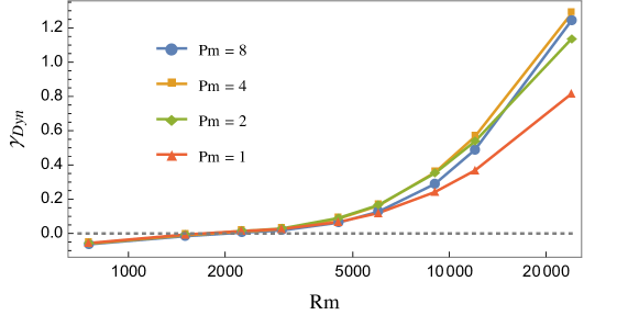
Figure 1: Growth rate $\gamma_{Dyn}$ of the mean field, $\bar{B}_{y}=\bar{B}_{y0}\left(z\right)e^{\gamma_{Dyn}t}$, as a function of magnetic Reynolds number at $\mathrm{Pm}=1,\,2,\,4\,\mathrm{and}\,8$.

Such behavior is illustrated in Fig. 1, which shows the growth rate $\gamma_{Dyn}$ of this dynamo instability. This is calculated by first evolving Eq. 3 to the homogenous equilibrium by artificially removing the nonlinear feedback, then introducing a very small ($\sim\!\!10^{-15}$) random mean field (with the amplitudes of $\bar{\bm{U}},\,\bar{B}_{x}$ 1/10 that of $\bar{B_{y}}$). (While it is possible to solve for the Floquet eigenspectrum directly, this is challenging due to the grid size.) Following the introduction of mean-field feedback there is a sustained period of exponential growth in $\bar{\bm{B}}$ for $\mathrm{Rm}\gtrsim 1500$. The observed eigenmodes are sinusoidal in $z$ (ensured by spatial homogeneity) although not generally the largest mode in the box, satisfy $B_{x}\ll B_{y}$ and seem to have $\bar{\bm{U}}=0$ . While it is certainly expected that $\gamma_{Dyn}$ increase strongly with $\mathrm{Rm}$ – fluctuations grow to a higher amplitude and there is less $\bar{\bm{B}}$ dissipation – its dependence on $\mathrm{Pm}$ is more interesting and suggestive. An increase in $\mathrm{Pm}$ implies more dissipation (through increasing $\bar{\nu}$), yet Fig. 1 shows that $\gamma_{Dyn}$ can increase, particularly at higher $\mathrm{Rm}$. In addition, $\tfrac{\partial}{\partial\mathrm{Rm}}\gamma_{Dyn}\left(\mathrm{Rm}\right)$ increases with $\mathrm{Pm}$, with potentially interesting consequences for the very high $\mathrm{Rm}$ limit. The instability is driven by the radial stress $\mathcal{M}_{x}$ causing an increase in $\bar{B}_{x}$, which in turn drives $\bar{B}_{y}$ through the $\Omega$ effect, $-q\bar{B}_{y}$ [see Eq. (4)]. The effect of the azimuthal stress $\mathcal{M}_{y}$ is always negative. This is identical to the dynamo mechanism studied in detail in Refs. Lesur and Ogilvie (2008a, b), and has strong similarities to exact nonlinear dynamo solutions at low $\mathrm{Rm}$ Rincon et al. (2007); Riols et al. (2013).

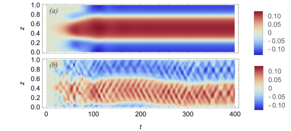
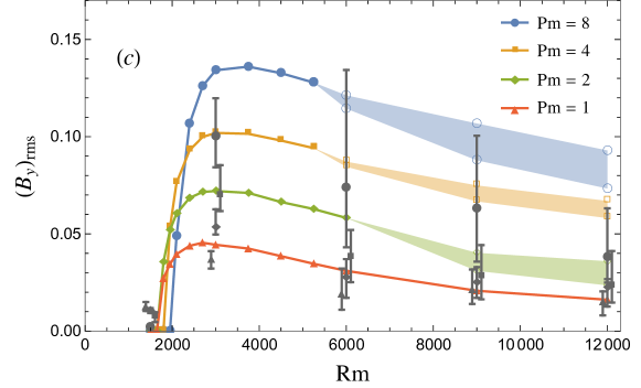
Figure 2: Evolution of $\bar{B}_{y}$ as a function of $\left(z,t\right)$ at $\mathrm{Pm}=4$ for (a) $\mathrm{Rm}=4500$, time-independent saturated state, and (b) $\mathrm{Rm}=12000$, time-dependent saturated state. (c) Magnitude of $\bar{B}_{y}$ as measured by $\left(\bar{B}_{y}\right)_{\mathrm{rms}}=\left(\tfrac{1}{L_{z}}\int dz\,\left|\bar{B}_{y}\right|^{2}\right)^{1/2}$ at saturation, as a function of $\mathrm{Rm}$ and $\mathrm{Pm}$. The shaded regions illustrate the approximate maxima and minima of the time-dependent $\bar{B}_{y}$ when the system did not reach a time-independent statistical equilibrium. Gray points (point styles as for CE2 results) illustrate the mean values of equivalent driven nonlinear simulations, with error-bars illustrating the approximate maxima and minima (the slight horizontal offset of $\mathrm{Pm}=1,\,4$ points is for clarity, the same Rm is used for all Pm).

Of more relevance to fully developed turbulence are the saturation characteristics of the dynamo instability. To save computation, we initialize with moderately strong random mean fields (amplitude of $\bar{B}_{y}\approx 0.01,$ $\bar{B}_{x}$ and $\bar{\bm{U}}$ initialized at 1/10 that of $\bar{B}_{y}$ – we have also studied initialization with the largest mode of the box obtaining similar results). As $\mathrm{Rm}$ is increased and homogenous equilibrium rendered unstable, the system saturates to a new CE2 equilibrium with a strong background $\bar{B}_{y}$ that varies on the largest scale in the box, as illustrated by the example in Fig. 2(a). As we increase $\mathrm{Rm}$ further, a second bifurcation occurs, at which the inhomogenous equilibrium appears to become unstable and the system transitions to a quasi-periodic time-dependent state. An example of this state, which occurs more readily at higher $\mathrm{Pm}$, is shown in Fig. 2(b). These two bifurcations – first to an inhomogenous state dominated by mean fields, then the loss of equilibrium of this state – bear a strong resemblance to the transitions seen in hydrodynamic plane Couette flow Farrell and Ioannou (2012), in which the second transition is associated with self-sustaining behavior. Such a self-sustaining process is not possible within our model due to the choice of 1-D mean-fields (as opposed to 2-D in Ref. Farrell and Ioannou (2012)), but the similarity as well as its $\mathrm{Pm}$ dependence is striking. Understanding physical mechanisms behind the loss of equilibrium may give useful insights into the self-sustaining dynamo that is so fundamental to zero net-flux turbulence.

This information is presented more compactly in Fig. 2(c), which illustrates the saturated $\bar{B}_{y}$ amplitude over a range of $\mathrm{Rm},\,\mathrm{Pm}$. The dependence of the saturated amplitude on $\mathrm{Pm}$ is enormous (contrary to previous results on the large scale dynamo Brandenburg (2009)), and can be well understood at low $\mathrm{Rm}$ using the linear properties of inhomogenous shearing waves Lesur and Ogilvie (2008a, b). Also shown is the mean azimuthal field $\overline{B_{y}\left(\bm{x}\right)}\left(z\right)\equiv(L_{x}L_{y})^{-1}\int dxdy\,B_{y}\left(\bm{x}\right)$ in driven nonlinear simulations (using statistically equivalent noise to that in CE2), which shows the same trends although amplitudes are somewhat smaller. These simulations are run at a resolution $64\times 128\times 64$ ($\mathrm{Rm}\leq 9000$) and $128\times 256\times 128$ ($\mathrm{Rm}=12000$) using the SNOOPY code Lesur and Longaretti (2007), and mean values are obtained through time averages from $t=200\rightarrow 400$. The large error-bars on these results illustrate how statistical simulation can be very profitable for observing such trends in data. Note that in contrast to most nonlinear simulation, the driving noise extends to the smallest scales available. Future work will explore how the turbulent dynamo changes as this is altered in both CE2 and nonlinear simulation Constantinou et al. (2014). Interestingly, there is a marked decrease in the saturated amplitudes at all $\mathrm{Pm}$ as $\mathrm{Rm}$ is increased. We have been unable to find a convincing physical mechanism to explain this effect, but note that it depends critically on the interaction of the fluctuating fields with $\bar{B}_{x}$. This illustrates that some important physical effects may be absent from the saturation mechanism proposed in Refs. Lesur and Ogilvie (2008a, b).

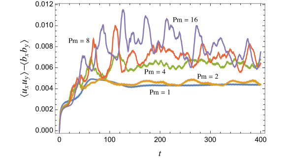
Figure 3: Angular momentum transport $\left\langle u_{x}u_{y}\right\rangle-\left\langle b_{x}b_{y}\right\rangle$ (including mean and fluctuating variables) as a function of time for $\mathrm{Rm}=12000$, $\mathrm{Pm}=1\rightarrow 16$.

In Fig. 3 we present the angular momentum transport as a function of time for the highest $\mathrm{Rm}$ calculations presented in Fig. 2. The increase in transport with $\mathrm{Pm}$ despite the increased dissipation is evident, suggesting a relationship between shearing box convergence problems Fromang et al. (2007); Fromang (2010) and the large scale dynamo. While the scaling is not so pronounced as self-sustained non-linear turbulence (see e.g., Ref. Fromang et al. (2007) figure 7), this is to be expected since the CE2 calculations are driven. The scaling in our driven nonlinear simulations (see Fig. 2, not shown in Fig. 3) is similar, although the overall transport level is a factor of $\sim\!\!1.5$ smaller. Note that the increase in transport is not primarily from the mean fields directly (e.g., through $\left<\bar{B}_{x}\bar{B}_{y}\right>$), but rather due to the fluctuations becoming more intense as a consequence of the stronger mean fields.

Discussion

Our primary motivation for this work has been to disentangle the important processes involved in MRI turbulence and dynamo. With this aim, we have enormously reduced the nonlinearity of the unstratified shearing box system, keeping only those interactions that involve the $k_{x}=k_{y}=0$ modes (the mean fields). This removes the usual turbulent cascade, although fluctuations are still swept to the smallest scales by the mean shear. Our primary result is that despite this huge simplification – the only nonlinearity is due to the mean field dynamo – the CE2 system displays qualitatively similar trends to fully developed MRI turbulence. In particular, a decrease in $\mathrm{Re}$ at fixed $\mathrm{Rm}$ ($i.e.,$ an increase in $\mathrm{Pm}$), causes an increase in angular momentum transport. This work illustrates the relationship of this trend to the large scale dynamo and facilitates future analytic studies to understand the primary causes for such behavior. The hope is that such understanding would allow extrapolation into the high and low Pm regimes that are so computationally challenging. In addition, statistical simulation (i.e., CE2) Farrell and Ioannou (2003); Marston et al. (2008) provides very clear information on the bifurcations between turbulent states of the system. We see two important bifurcations as $\mathrm{Rm}$ is increased: the first is the transition from stable homogenous turbulence to a stable inhomogenous equilibrium with strong mean-fields (the dynamo instability), the second a loss of stability of the inhomogenous equilibrium and transition to a near-periodic time-dependent state. Given the strong dependence of both the saturated states and the second bifurcation on $\mathrm{Pm}$, as well as the marked similarity to studies of plane Couette flow Farrell and Ioannou (2012), it seems likely that further study of this dynamo instability will yield important insights into the fundamental nature of the MRI system.