SPIDER X – Environmental effects in central and satellite early-type galaxies through the stellar fossil record

Abstract

A detailed analysis of how environment affects the star formation history of early-type galaxies (ETGs) is undertaken via high signal to noise ratio stacked spectra obtained from a sample of $20,977$ ETGs (morphologically selected) from the SDSS-based SPIDER survey. Two major parameters are considered for the study: the central velocity dispersion ($\sigma$), which relates to local drivers of star formation, and the mass of the host halo, which relates to environment-related effects. In addition, we separate the sample between centrals (the most massive galaxy in a halo) and satellites. We derive trends of age, metallicity, and [$\alpha$/Fe] enhancement, with $\sigma$. We confirm that the major driver of stellar population properties in ETGs is velocity dispersion, with a second-order effect associated to the central/satellite nature of the galaxy. No environmental dependence is detected for satellite ETGs, except at low $\sigma$ – where satellites in groups or in the outskirts of clusters tend to be younger than those in the central regions of clusters. In contrast, the trends for centrals show a significant dependence on halo mass. Central ETGs in groups (i.e. with a halo mass $>10^{12.5}M_{\odot}$) have younger ages, lower [$\alpha$/Fe], and higher internal reddening, than “isolated” systems (i.e. centrals residing in low-mass, $<10^{12.5}M_{\odot}$, halos). Our findings imply that central ETGs in groups formed their stellar component over longer time scales than “isolated” centrals, mainly because of gas-rich interactions with their companion galaxies.

1 Introduction

Despite many observational and theoretical efforts over the past thirty years, the population of early-type galaxies (ETGs) remains a challenge of modern cosmology. Galaxy formation and evolution is an extremely variegated discipline, involving complex “internal” processes, such as the transformation of gas into stars, feedback processes from, e.g., active galactic nuclei and supernovæ, as well as “external” processes, such as interactions among galaxies and between galaxies and their environment (e.g. ram-pressure stripping induced by the hot intra-cluster medium). Despite this complexity, most of the observed properties of ETGs appear very homogeneous, showing tight correlations with a single key observable, central velocity dispersion (see, e.g. Bernardi et al., 2003). Such correlations involve structural parameters (namely, the scale radius and mean luminosity density within that radius), also known as Fundamental Plane relation (Djorgovski & Davis, 1987; Dressler et al., 1987), as well as the underlying stellar populations (e.g. age and chemical composition).

In the last twenty years, our knowledge of the stellar populations of ETGs has advanced, thanks to improvements in the spectroscopic and photometric observations available (e.g., Trager et al., 2000; Thomas et al., 2005; Gallazzi et al., 2006; Bernardi et al., 2005; Smith et al., 2007; Pasquali et al., 2010; Zhu, Blanton, Moustakas, 2010; Thomas et al., 2010; Harrison et al., 2011), as well as advances in the theoretical modelling of unresolved stellar populations (e.g., Worthey, 1994; Bruzual & Charlot, 2003; Maraston, 2005; Vazdekis et al., 2012). It is now widely accepted that both metallicity and the abundance of the $\alpha$-elements (in particular the ratio [Mg/Fe]) increase with galaxy mass, the main driver of these correlations being the central velocity dispersion, $\sigma$ (i.e. the central potential well) of a galaxy (Bernardi et al., 2003), or its dynamical mass (Gallazzi et al., 2006; Chang et al., 2006). The stellar metallicity-$\sigma$ relation can be understood because most of the massive systems retain more efficiently the heavy elements from exploding supernovæ within their deeper potential well (Larson, 1974; Arimoto & Yoshii, 1987). Since $\alpha$ elements are released during the explosion of short-lived massive stars (type II supernovæ), in contrast to iron, that is mainly produced by type Ia supernovæ, the ratio [$\alpha$/Fe] is believed to serve as a proxy of the star-formation time scale of a galaxy. Therefore, the [$\alpha$/Fe]-$\sigma$ relation can be interpreted as a trend towards shorter, more efficient star formation in the most massive ETGs (see, e.g., Thomas et al., 1999, 2005). Regarding stellar ages, early studies found no significant correlation with galaxy mass (e.g. Trager et al. 2000; Kuntschner et al. 2001), while more recent works have found the age to increase with central velocity dispersion, especially at low velocity dispersion. The trends of age and metallicity with mass are not limited to the central regions of ETGs, probed by spectroscopic studies, but also apply to their overall (i.e. aperture-integrated) stellar populations, as implied by the FP relation (La Barbera et al., 2010b). In addition to age, metallicity, and abundance ratios, the (unresolved) stellar populations of ETGs have also been recently found to feature a varying stellar Initial Mass Function (IMF), through the analysis of gravity-sensitive features in their spectra. A significant correlation is also found in place, between IMF slope and velocity dispersion, with massive ETGs having enhanced fractions of dwarf-to-giant stars with respect to a “standard”, Kroupa-like IMF (Cenarro et al., 2001; van Dokkum & Conroy, 2010; Conroy & van Dokkum, 2012b; Ferreras et al., 2013; La Barbera et al., 2013; Spiniello et al., 2014).

Although galaxy mass (or more precisely, velocity dispersion) is found to be the primary driver of the stellar population properties of ETGs, these properties are also affected by the environment where galaxies reside. Several studies have analysed the dependence of age, metallicity, and [$\alpha$/Fe], on “local” environment, characterised either by the density of neighbouring galaxies, the distance to the centre of the host group/cluster, or by splitting galaxies into those residing in galaxy groups and those in the “field” (e.g. Bernardi et al. 2003; Thomas et al. 2005; Bernardi et al. 2006; Annibali et al. 2007; Clemens et al. 2009; Thomas et al. 2010; Pasquali et al. 2010; Zhu, Blanton, Moustakas 2010; Cooper et al. 2010). These works have all found that galaxies in low-density regions have younger luminosity-weighted ages than their cluster counterparts, with age differences of $\sim 1$–$2$ Gyr (e.g. Guzmán et al. 1992; Trager et al. 2000; Kuntschner et al. 2002; Terlevich & Forbes 2002; Thomas et al. 2005; Bernardi et al. 2006; Clemens et al. 2009). Such differences also exist when considering ETGs in high-density, low-velocity dispersion systems, such as the Hickson Compact Groups (de La Rosa et al., 2007). In contrast, discordant results have been reported in the literature regarding trends between environment and metallicity. Bernardi et al. (2006) found no detectable difference in the metallicity of field and cluster ETGs, whereas other studies, e.g. Thomas et al. (2005); de La Rosa et al. (2007); Clemens et al. (2009) found evidence for galaxies in dense environments to be less metal rich than those in the field. One possible cause of these discrepancies is the significant dependence of the internal metallicity gradients of ETGs on environment (see La Barbera et al. 2011 and references therein), with different studies targeting different apertures for the stellar population analysis. The environmental dependence of [$\alpha$/Fe] has been addressed less frequently in the literature than age and metallicity trends, mostly because of the lack of stellar population models, based on empirical stellar libraries that cover a range in age, metallicity, and [$\alpha$/Fe]. Bernardi et al. (2006) found ETGs at high density to be more $\alpha$-enhanced than those at low density, indicative of a shorter formation time scale of their stars. Thomas et al. (2005) found that the fraction of “rejuvenated” objects, having young ages and lower [$\alpha$/Fe], increases from high- to low-density regions. However, these trends with environment are biased by galaxy stellar mass, as it is well known that more massive galaxies inhabit denser regions of the Universe (Dressler, 1980). Such a coupling between galaxy stellar mass and environment has to be carefully taken into account in order to single out the effects of environment alone (see, e.g., Pasquali et al., 2009; Cooper et al., 2010).

Although local density is an intuitive way to describe the environment where a galaxy resides, it is not necessarily the most effective way to characterise it. In the current picture (e.g. Croton et al. 2006; De Lucia et al. 2006), two main paths of galaxy formation and evolution can be envisioned. Galaxies can be either “centrals” in a surrounding dark-matter halo, or “satellites”, being accreted onto the halo during its hierarchical build-up. Centrals can keep accreting hot gas from the halos they are embedded in, whereas satellites are believed to be deprived of their gas reservoir by their host halo. Therefore, splitting galaxies into centrals and satellites is a more natural way to compare observations and theory. Another interesting approach to characterise the environment is that of using the shape of the velocity distribution of galaxies in a group (see, e.g., Ribeiro et al. 2013). Despite the fact that several studies have analysed the dependence of stellar populations of ETGs on local environment, there has been no detailed stellar population study of the two populations of satellite and central ETGs individually. This is indeed the main focus of the present work. By analysing stacked spectra obtained from a large sample of morphologically selected ETGs from the SDSS-based SPIDER survey (La Barbera et al., 2010a), we explore how the stellar populations of central and satellite ETGs – namely the age, metallicity, [$\alpha$/Fe], and internal extinction – depend on the “global” environment (i.e. the mass of the parent halo) where they reside. We compare galaxy properties at fixed velocity dispersion, in order to single out the effect of galaxy mass and environment. The present analysis complements  Pasquali et al. (2010, hereafter PGF10), differing from it in several regards: (i) we analyse here only the population of morphologically selected ETGs; (ii) the properties of galaxies are compared at fixed velocity dispersion, rather than fixed galaxy stellar mass; (iii) we study here also the environmental dependence of [$\alpha$/Fe] and internal extinction, in addition to age and metallicity (as in PGF10). Throughout the present work, we adopt a cosmology with $\Omega_{\rm m}=0.3$, $\Omega_{\Lambda}=0.7$, and H${}_{0}=100h$  km s^-1 Mpc^-1, with $h=0.7$.

2 Data

2.1 Sample

The SPIDER sample consists of 39,993 nearby (0.05$<$z$<$0.095) ETGs selected from Data Release 6 of the Sloan Digital Sky Survey (SDSS-DR6; Adelman-McCarthy et al. 2008). Following  Bernardi et al. (2003), ETGs are defined as bulge-dominated systems with passive spectra. The former is constrained via the SDSS attribute $fracDev_{r}\!>\!0.8$, where $fracDev_{r}$ measures the fraction of galaxy light better fitted by a de Vaucouleurs profile, rather than an exponential law. For the latter, we use the SDSS attribute $eClass\!<\!0$, where $eClass$ indicates the spectral type of a galaxy based on a principal component analysis decomposition. Galaxies are selected to have absolute $r$-band Petrosian magnitudes brighter than $r_{Petr}=-20$, corresponding to the observed separation between the two families of bright and ordinary ellipticals (Capaccioli, Caon & D’Onofrio, 1992; Graham & Guzmán, 2003). As detailed in La Barbera et al. (2010a, hereafter Paper I), for a subsample of $5,080$ ETGs there is also NIR ($YJHK$) photometry available from UKIDSS-DR3. All galaxy images, in the $grizYJHK$ wavebands, were homogeneously fitted with two-dimensional PSF-convolved Sérsic models, providing structural parameters, namely the effective radius, $\rm R_{\rm e}$, the Sérsic (shape-parameter), $n$, and the total luminosity, from $g$ through $K$. All SPIDER ETGs have spectra as well as central velocity dispersions, $\sigma$, available from SDSS. The spectra, ranging from $3800$ to $9200$ Å, have been retrieved from SDSS-DR7 (Abazajian et al., 2009), de-redshifted to a common rest-frame and corrected for foreground Galactic extinction (see Paper I).

For the present study, we rely on a subsample of SPIDER ETGs, selected as follows. Following La Barbera et al. (2013, hereafter Paper VIII), we select objects with: (i) $\sigma>100$  km s^-1($N_{ETGs}=38,447$); (ii) low internal extinction ($E(B\!-\!V)<0.1$ mag; $N_{ETGs}=33,095$); and (iii) spectra whose $S/N$ ratio computed per Å in the H$\beta$ region is higher than 14, 27 and 21 at $\sigma$ = 100, 200 and 300  km s^-1, respectively (thus excluding those objects within the lowest quartile of the $S/N$ distribution in a given $\sigma$ bin; $N_{ETGs}=24,781$). Since ETGs in the SPIDER sample are defined through the SDSS $fracDev_{r}$ parameter, which is a proxy of bulge fraction, the sample is affected by some amount of contamination (up to $17\%$, see Paper I) from late-type galaxies (LTGs) with a prominent bulge. Due to the morphology–density relation (Dressler, 1980), the contaminant fraction is expected to increase towards lower density regions, potentially introducing a systematic trend in the study of stellar populations as a function of environment.

To avoid this, we define a sample of bona-fide, morphologically selected, ETGs. Firstly, we take advantage of the publicly available catalogue of the Galaxy Zoo project, that provides the morphological classification of nearly 900,000 SDSS galaxies (Lintott et al., 2011). Except for a few cases (72 out of $39,993$ galaxies), inspected visually by ourselves, SPIDER ETGs have a Galaxy Zoo classification. We use the fraction of votes for ellipticals, p_ell, spirals (both clock-wise and anti-clock-wise), p_sp, and edge-on spirals, p_edge. Face-on LTGs have p_sp $>$ p_ell, while edge-on disks have p_edge $>$ p_ell. Under these criteria, our main SPIDER sample contains $1,806$ face-on LTGs, $3,545$ edge-on LTGs (4.5 and 8.9 % of the total, respectively), and $712$ objects (1.8 %) tagged as unclassified/mergers. Since some early-type spirals (Sa/SBa) are not present in the Galaxy Zoo classification, we apply a further selection criterion based on the quality of the two-dimensional Sérsic fits to the surface brightness distribution. For each fit, the $\chi^{2}$ is measured as the rms of the residuals from the fit. High values of $\chi^{2}$ usually correlate with the presence of faint morphological features, such as disks or spiral arms (see, e.g., figure 6 of Paper I). We use the fitting results for the g-band images, which are expected to be sensitive to the presence of young stellar components. As expected, the $\chi^{2}$ correlates with the Galaxy Zoo classification. Edge-on and face-on LTGs have a median $\langle\chi^{2}\rangle$ of $1.31$ and $1.41$, respectively, while the remaining sample has a median $\langle\chi^{2}\rangle=1.02$ (consistent with figure 5 of Paper I), with a standard deviation $\sigma_{\chi^{2}}=0.17$. We define as residual contaminants those objects not flagged as LTGs from the Galaxy Zoo classification, but residing in the high-end tail of the $\chi^{2}$ distribution, i.e. $\chi^{2}>\langle\chi^{2}\rangle+3\sigma_{\chi^{2}}$. This selection excluded an additional $852$ objects (2.1 %) of the main sample. Out of $24,781$ galaxies selected with the same criteria as in Paper VIII (see points i–iii above), $3,126$ are removed after the morphological selection described above, resulting in a sample of $21,655$ bona-fide ETGs. Finally, $20,977$ (out of $21,655$) ETGs have environment defined, and are binned into five subsamples of ETGs residing in different environments, as detailed below.

The SPIDER sample is approximately complete down to $r_{Petr}=-20$, which is one of the main criteria imposed to select ETGs (see above, and Paper I for details). Because of the scatter in the $\sigma$–luminosity relation, this $r$-band selection may induce some incompleteness at low velocity dispersion. To quantify it, we have estimated the fraction of ETGs excluded by the $r_{Petr}$ cut, defined as $f_{>r}$, as a function of $\sigma$. We find $f_{>r}\sim 10\%$ at $\sigma\sim 140$  km s^-1, increasing up to $\sim 25\%$ at $110$  km s^-1. We notice that $f_{>r}$ is an upper estimate of incompleteness, as galaxies fainter than $-20$ are ordinary rather than bright ETGs (see below), i.e. do not necessarily belong to the population of galaxies we want to target. Finally, we remark that although incompleteness might affect the low-$\sigma$ trends of stellar population properties, it does not affect the relative comparison of these properties with environment at fixed $\sigma$, which is the main goal of this paper.

2.2 Environment

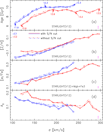
Figure 7: Comparison of trends of stellar population properties of ETGs obtained with (solid) and without (dot-dashed) selecting SDSS spectra with best $S/N$ ratio (see the text). Notice that solid curves and labels are the same as in Fig. 3.

We characterise the environment where ETGs reside by means of the updated catalogue of galaxy groups of Yang et al. (2007, hereafter Y07). The difference between the updated version and the one defined in Y07 is the area used, i.e. SDSS-DR7 (Abazajian et al., 2009) rather than DR4 (Adelman-McCarthy et al., 2006). The catalogue is constructed by applying the halo-based group finder algorithm of Yang et al. (2005) to the New York University Value-Added Galaxy Catalogue (NYU-VAGC, Blanton et al. 2005) extracted from SDSS-DR7. From the NYU-VAGC Main Galaxy Sample, Y07 extracted all galaxies with an $r$-band apparent magnitude brighter than $r$ = 18 mag, in the redshift interval 0.01 $\leq z\leq$ 0.20 and with a redshift completeness $C_{z}>$ 0.7. Three samples were built with the selected galaxies: sample I, which only uses the $593,736$ galaxies with measured redshifts from the SDSS; sample II based on the $593,736$ galaxies with measured redshifts from SDSS, plus an additional $3,115$ galaxies with SDSS photometry and redshifts from different sources; sample III which lists $36,602$ additional galaxies lacking a redshift due to fibre collisions, but being assigned the redshift of the nearest neighbour. For our analysis, we rely on sample II, where galaxies are split into centrals (defined as the most massive group members on the basis of galaxy stellar mass) and satellites (all group members that are not centrals). The dark matter halo mass, M_h, provided in this sample for each galaxy group, is based on the ranking of the group total stellar mass, where galaxy stellar masses are derived from the relationship between stellar mass-to-light ratio and colour of Bell et al. (2003). The method of Y07 can only assign halo masses to groups more massive than M${}_{\rm h}\sim$10${}^{12}~{}h^{-1}$M_⊙, and with one or more members brighter than M${}_{\rm r}-5\log h=-19.5$ mag (K-corrected to $z$ = 0.1). For M${}_{\rm h}\lower 2.15277pt\hbox{$\;\buildrel>\over{\sim}\;$}$10${}^{12}~{}h^{-1}$M_⊙, the Y07 group finder successfully selects more than 90$\%$ of all “true” halos (see Y07 for details), almost independent of their richness and with only a very weak dependence on halo mass. For less massive groups, Yang, Mo & van den Bosch (2008) used the relationship between the stellar mass of central galaxies and the halo mass of their groups to estimate the halo mass of single central galaxies down to M${}_{\rm h}\sim$ 10${}^{11}~{}h^{-1}$M_⊙. Y07 assessed the uncertainty on M_h by measuring halo masses for a mock group catalogue and comparing them to true dark-matter halo masses. The scatter on M_h  has been found to range from $\sim 0.35$ dex at M_h$\sim 13.5$–$14$ to $\sim 0.2$ dex at high- (M_h$\sim 14.6$) and low-(M_h$\sim 12$) halo masses (see their fig. 7). We discuss the possible effect of the M_h  uncertainty on our results in Sec. 4.1.

Out of $21,655$ bona-fide ETGs selected for the present study (see above), $20,977$ ETGs are in sample II of the Y07 group catalogue, and are thus classified as centrals ($N=15,572$) or satellites ($N=5,425$). Fig. 1 shows the mass distribution of the parent halos where ETGs reside. Satellites span a wider range of halo mass, from $\log($M${}_{\rm h}/$M${}_{\odot})$$\sim 13$, i.e. the mass scale of groups of galaxies, to $\log($M${}_{\rm h}/$M${}_{\odot})$$\sim 15$, i.e. massive galaxy clusters. On the contrary, most centrals ($\sim 89\,\%$) have $\log($M${}_{\rm h}/$M${}_{\odot})$ below $13$, reflecting the higher number density of low- to high-mass halos. For $\log($M${}_{\rm h}/$M${}_{\odot})$$<12.5$, centrals are indeed “isolated” galaxies, as suggested by the fact that only a minor fraction, $\sim 2\,\%$, of satellite ETGs reside in halos with masses below this value. In general, considering the entire sample II of Y07 we found $<9\%$ of all groups with M_h$<12.5$ to have (both early- and late-type) satellites, with only $1\%$ of them having more than one satellite. Hence, we split central ETGs into two subsamples, having low halo mass ($<12.5$), that can be regarded as “isolated” galaxies (hereafter sample C1), and high halo mass ($\geq 12.5$), i.e. groups’ central ETGs (hereafter sample C2), respectively (see red–dashed vertical line in the Figure). These two subsamples include $68\,\%$ ($N=10,534$) and $32\,\%$ ($N=5,038$) of all central ETGs ($N=15,572$), respectively. In the satellite ETG population, we define three subsamples, namely, two subsamples comprising low- ($\log($M${}_{\rm h}/$M${}_{\odot})$$<14$; $N=2,945$, sample S1) and high- ($\log($M${}_{\rm h}/$M${}_{\odot})$$\geq 14$; $N=1,582$, sample S2) halo-mass, at small cluster-centric projected radii ($R\leq 0.5\,R_{200}$); and an additional third subsample consisting of satellite ETGs in the outer group regions ($R>0.5\,R_{200}$), regardless of group halo mass ($N=898$, sample S3). Notice that S3 is too small for a further subdivision according to halo mass. To simplify our notation, we refer to satellites at low and high halo mass as group- and cluster- satellites, respectively. In summary, we define five subsamples of ETGs residing in different environments, namely four subsamples (either centrals or satellites) defined with respect to halo mass, and an additional subsample of satellites that lie in the external regions of the host halo. Notice that we adopt a different threshold in halo mass to split centrals and satellites, as our goal is not to compare satellites with centrals, but to analyse the effect of the halo mass on each population separately. The general details of these subsamples are summarised in Tab. 1.

Table 1: Samples of ETGs residing in different environments. Each sample is identified by a label (col. 1). The definition of environment is summarised in col. 2, while col. 3 gives the sample size.

sample	environment	$N$
(1)	(2)	(3)
$\rm C1$	centrals, $\log($M${}_{\rm h}/$M${}_{\odot})$$<12.5$	$10,534$
$\rm C2$	centrals, $\log($M${}_{\rm h}/$M${}_{\odot})$$\geq 12.5$	$5,038$
$\rm S1$	satellites, $R/R_{200}<0.5$, $\log($M${}_{\rm h}/$M${}_{\odot})$$<14$	$2,945$
$\rm S2$	satellites, $R/R_{200}<0.5$, $\log($M${}_{\rm h}/$M${}_{\odot})$$\geq 14$	$1,582$
$\rm S3$	satellites, $R/R_{200}\geq 0.5$	$898$

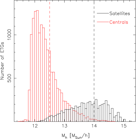
Figure 1: (Logarithmic) halo mass distribution of our sample of $20,977$ bona-fide ETGs. The histograms of galaxies classified as centrals and satellites in the updated Y07 group catalogue (see Sec. 2.2) are shown in red and black, respectively. The vertical dashed lines mark the threshold values of the halo mass that split centrals (red) and satellites (black) (see the text for details).

Table 2: Properties of stacked spectra for samples of ETGs residing in different environments (see labels in Tab. 1), i.e. central ETGs with low- and high- host halo mass (cols. 1–3 and 4–6, respectively), and satellite ETGs with low- (cols. 7–9) and high- (cols. 10–12) M_h, and at large projected group-centric distances (cols. 13–15). For each sample, the Table lists the velocity dispersion bins with their $\sigma$ range (in  km s^-1, cols. 1, 4, 7, 10, 13), the number of ETGs, $\rm N$, in each bin (col. 2, 5, 8, 11, 14), and the $S/N$ ratio per Å of the corresponding stacked spectrum (cols. 3, 6, 9, 12, 15).

C1			C2			S1			S2			S3
$\sigma$	$\rm N$	$S/N$	$\sigma$	$\rm N$	$S/N$	$\sigma$	$\rm N$	$S/N$	$\sigma$	$\rm N$	$S/N$	$\sigma$	$\rm N$	$S/N$
(1)	(2)	(3)	(4)	(5)	(6)	(7)	(8)	(9)	(10)	(11)	(12)	(13)	(14)	(15)
$100$–$110$	$630$	$371$	$100$–$130$	$101$	$180$	$100$–$110$	$173$	$194$	$100$–$110$	$53$	$117$	$100$–$110$	$52$	$107$
$110$–$120$	$1093$	$493$	$130$–$140$	$94$	$174$	$110$–$120$	$264$	$238$	$110$–$120$	$110$	$158$	$110$–$120$	$73$	$131$
$120$–$130$	$1387$	$590$	$140$–$150$	$189$	$233$	$120$–$130$	$321$	$281$	$120$–$130$	$139$	$190$	$120$–$130$	$108$	$169$
$130$–$140$	$1422$	$609$	$150$–$160$	$274$	$289$	$130$–$140$	$359$	$312$	$130$–$140$	$145$	$186$	$130$–$140$	$115$	$185$
$140$–$150$	$1430$	$624$	$160$–$170$	$402$	$354$	$140$–$150$	$329$	$306$	$140$–$150$	$146$	$214$	$140$–$150$	$110$	$184$
$150$–$160$	$1256$	$617$	$170$–$180$	$473$	$403$	$150$–$160$	$300$	$308$	$150$–$160$	$139$	$196$	$150$–$160$	$91$	$161$
$160$–$170$	$1150$	$617$	$180$–$190$	$532$	$428$	$160$–$170$	$285$	$312$	$160$–$170$	$156$	$244$	$160$–$170$	$92$	$197$
$170$–$180$	$793$	$516$	$190$–$200$	$526$	$443$	$170$–$180$	$216$	$288$	$170$–$180$	$142$	$230$	$170$–$180$	$53$	$161$
$180$–$190$	$566$	$447$	$200$–$210$	$554$	$471$	$180$–$190$	$195$	$279$	$180$–$190$	$115$	$214$	$180$–$190$	$53$	$141$
$190$–$200$	$356$	$372$	$210$–$220$	$446$	$440$	$190$–$200$	$158$	$252$	$190$–$200$	$109$	$206$	$190$–$210$	$70$	$205$
$200$–$210$	$194$	$277$	$220$–$230$	$393$	$438$	$200$–$210$	$112$	$229$	$200$–$210$	$78$	$200$	$210$–$230$	$42$	$148$
$210$–$220$	$123$	$210$	$230$–$240$	$335$	$423$	$210$–$220$	$86$	$220$	$210$–$220$	$65$	$169$
$220$–$230$	$59$	$160$	$240$–$250$	$234$	$341$	$220$–$230$	$58$	$159$	$220$–$230$	$55$	$165$
$230$–$250$	$58$	$177$	$250$–$260$	$174$	$299$	$230$–$250$	$60$	$203$	$230$–$250$	$63$	$222$
			$260$–$270$	$118$	$251$				$250$–$280$	$51$	$211$
			$270$–$280$	$72$	$223$
			$280$–$290$	$57$	$180$
			$290$–$310$	$52$	$206$

2.3 Stacked spectra

Following the same procedure as in Paper VIII, the spectroscopic analysis of the sample is based on stacked spectra, providing a high $S/N$ ($>100$ Å^-1). For each environment-related subsample, the spectra are stacked in bins of velocity dispersion, starting from $\sigma=100$  km s^-1, with a minimum bin size, $\delta_{\sigma}$, of 10  km s^-1. This size is chosen to match the error on the measurement of the velocity dispersion over the range 100  km s^-1$\leq\sigma\leq$ 300  km s^-1. When necessary, the bin size, $\delta_{\sigma}$, is increased adaptively, in steps of $10$  km s^-1, up to a maximum value of $30$  km s^-1, in order to have a minimum of $40$ spectra per bin. Bins that do not fulfil these constraints (i.e. $N\geq 40$ for $\delta_{\sigma}\leq 30$  km s^-1) are not included in the analysis. Adopting a minimum number of $40$ spectra in each bin ensures that the $S/N$ ratio is large for all stacked spectra. A maximum bin size of $30$  km s^-1 is adopted because the aim of this work is to quantify the effect of “global” (large-scale) environment with respect to the “local” (galaxy scale) driver of the star formation histories of ETGs. A good proxy for the latter is central velocity dispersion (Bernardi et al., 2005). The spectra in each $\sigma$ bin are convolved to match the upper $\sigma$ limit of the bin. Subsequently, for each sample, and each $\sigma$ bin, we median stack the available spectra, considering only pixels with no SDSS flag raised. Noise in stacked spectra is computed as the uncertainty of median flux values, accounting for the actual distribution of flux values at each wavelength. This procedure results in a total of 72 stacked spectra, corresponding to central and satellite ETGs residing in different environments, and over a velocity dispersion range from $\sim 100$ to $\sim 250$  km s^-1 (with the upper value depending on the sample). Relevant properties of all stacks are summarised in Tab. 2, where we report the range of each $\sigma$ bin, the number of ETGs per bin, and the median $S/N$ ratio of the stacks, computed in the central passband of the age-sensitive $\rm H\beta$ line (from $4840$ to $4880$ Å). The stacked spectra feature a remarkably high $S/N$, larger than $\sim 100$Å^-1 for all bins, with a maximum of $\sim 300$Å^-1 for central ETGs at low halo mass (see Tab. 2).

3 Stellar population properties

This paper focuses on estimating stellar population properties, i.e. $Age$, total metallicity, $[Z/H]$, and $\alpha$-to-iron abundance variations, [$\alpha$/Fe], using high $S/N$ stacked spectra to robustly derive the contribution of galaxy-scale (via velocity dispersion) and halo-scale (via halo mass) physics to the star formation histories of ETGs. In the following, we describe the procedure followed to obtain $Age$ and $[Z/H]$  (Sec. 3.1), and [$\alpha$/Fe] (Sec. 3.2).

3.1 Age and metallicity

We fit each stacked spectrum with the spectral fitting code STARLIGHT (Cid Fernandes et al., 2005). For a given input observed spectrum, STARLIGHT determines the best-fitting linear combination of a basis set of models. The basis comprises $N_{\rm SSP}$ simple stellar populations (hereafter SSP). Each SSP is characterised by a fixed age and chemical composition. The best fitting solution is described by the relative light-weighted contribution, $\{x_{j}\}\ (j=1,\cdots,N_{\rm SSP})$, that corresponds to each of the SSPs in the basis. In addition, STARLIGHT provides an estimate of the internal reddening, $\rm A_{V}$, of the input spectrum, by including an extinction law in the fitting process. We adopt here a set of $108$ input SSPs from the MILES galaxy spectral library (Vazdekis et al., 2010), with $27$ log-spaced ages ranging from $0.5$ to $\sim 17.78$ Gyr, four metallicities $[Z/H]=\{-0.71,-0.40,0.00,+0.22\}$, and a Kroupa Universal Initial Mass Function (IMF). MILES SSPs cover the spectral range $3525$–$7500$ Å, with a spectral resolution of 2.3 Å (Falcón-Barroso et al., 2011) . Hence, they are well suited to analyse SDSS spectra, whose spectral resolution is $\sim$ 2.3 Å  FWHM, at $\lambda\sim 5350$ Å (see, e.g., Paper VIII). MILES models are based on stellar spectra in the solar neighbourhood (the MILES stellar library, see Sánchez-Blázquez et al. 2006a), which are solar-scaled only at solar and super-solar metallicities, having [$\alpha$/Fe]$>0$ at low metallicities ($[Z/H]<-0.4$). In practice, this deviation from solar-scale is not relevant for the present study, as even in our lowest $\sigma$ stacks, the metallicities are slightly sub-solar ($[Z/H]$$>-0.15$). Notice also that although we include SSPs in our basis with ages older than the current estimate of the age of Universe (13.75 Gyr, Hinshaw et al., 2013), the derived $Age$ estimates from STARLIGHT do not exceed $11$ Gyr for any of our stacks (see below), i.e. consistent with the age of the Universe at the median redshift ($z\sim 0.07$) of our sample of ETGs ($\sim 12.5$ Gyr with the adopted cosmology). More importantly, we emphasise that the zero-point $Age$ calibration of stellar population models remains uncertain at present, suggesting that relative (rather than absolute) age differences should be considered in stellar population synthesis studies. Regarding internal extinction, a Cardelli, Clayton, Mathis (1989) extinction law is adopted, suitable for systems with low levels of star-formation, like ETGs. Spectral fitting is performed over the spectral range from $4000$ to $5700$ Å. We exclude regions bluer than $4000$ Å as they are more sensitive to (i) small fractions of young stars in a stellar population, and (ii) non-solar abundance ratios of chemical elements in the stellar atmospheres, that might bias the estimate of age and metallicity when relying on (nearly) solar-scaled (MILES) stellar population models. We also exclude from the fitting window those regions potentially affected by (nebular) emission, i.e. $H{\delta}$ ($4092$–$4112$ Å), $H{\gamma}$ ($4330$–$4350$ Å), $H{\beta}$ ($4848$–$4874$ Å), and $[OIII]$ ($4940$–$5028$ Å). Wavelengths longer than $5700$ Å are also excluded from the fitting as they include several features (e.g. Na absorption at $5900$ and $8200$ Å, as well as TiO bands) that are especially sensitive to the stellar IMF (Paper VIII). While a systematic variation of the IMF with velocity dispersion has been detected in ETGs (e.g. Conroy & van Dokkum 2012a; Ferreras et al. 2013; Spiniello et al. 2014; Paper VIII), we leave the issue of a possible dependence of the IMF on environment to a future paper. To allow for a better comparison with previous works, we derive the correlation of stellar population properties with velocity dispersion assuming a constant, Kroupa, IMF. Fig. 2 shows an example of the best-fitting spectrum produced by STARLIGHT, for one of our stacks (corresponding to sample C2, with $\sigma\sim 200$  km s^-1), with the regions excluded from the fit in grey. Residuals are at the level of a few percent throughout the whole spectral range fitted.

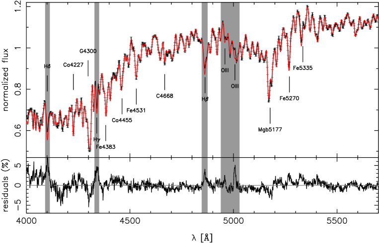
Figure 2: Example of a STARLIGHT fit for one of our stacked spectra, drawn from sample C2, with $\sigma\sim 200$  km s^-1. The upper panel shows the stacked spectrum (black curve), the STARLIGHT best-fit (red curve), one-sigma uncertainties of the flux values (grey error bars). The regions excluded from the fit because of possible contamination from nebular emission are shaded in grey. Some prominent absorption features are marked with vertical ticks and labelled. The lower panel plots the relative residuals with respect to the fit.

For each stack, we run STARLIGHT by first smoothing the basis SSP models to match the wavelength-dependent resolution of the SDSS spectrograph (see Paper VIII for details) as well as the velocity dispersion of the stack under study. Hence, for a given property, $Y$, (either age or metallicity), we estimate its luminosity-weighted value, $Y_{L}$, as

$$Y_{L}=\frac{\sum Y\times x_{j}}{\sum x_{j}},$$ (1)

where the sum extends over all the basis SSPs. $[Z/H]$ is obtained directly from Eq. 1, whereas for $Age$, we first estimate the logarithmic luminosity-weighted value, and then convert it to linear units. The uncertainties on $Age$ and $[Z/H]$ are derived via a bootstrap procedure, where STARLIGHT is run for $200$ realisations of the input spectrum, randomly modifying each time the flux values according to their uncertainties. The errors on $Age$ and $[Z/H]$ are given as the widths of the distributions of these parameters among the different realisations. Due to the high $S/N$ of the stacks, the typical random error on $Age$ is $\sim 2$%, while for $[Z/H]$ the typical uncertainty amounts to $\sim 0.006$ dex (computing median values over all choices of $\sigma$/environment).

We notice that a potentially important issue for the present study is that we estimate $Age$ and $[Z/H]$  with (nearly) solar-scaled stellar population models. For the $\alpha$-enhanced stellar populations expected in massive ETGs, the use of solar-scaled models might bias the inferred estimate of age and metallicity. More importantly, any dependence of [$\alpha$/Fe] on environment might also introduce a systematic variation of age and metallicity – when derived with solar-scaled models. Since at the moment there is no set of SSP models, based on empirical stellar spectra, that take [$\alpha$/Fe]  properly into account, one way to overcome this problem would be to estimate age and metallicity from single spectral features (like $\rm H\beta$ and the total metallicity indicator $\rm[MgFe]^{\prime}$), that are believed to be independent of [$\alpha$/Fe]. The main drawback of this approach is that one does not take full advantage of the information encoded in a galaxy spectrum, hampering a detailed study of the SFH. Based on these considerations, in the present work we adopt the following approach. Our reference estimates of age and metallicity are those obtained with widely used, well referenced, solar-scaled MILES models. However, in App. A, we also adopt a preliminary version of MILES SSPs with varying [$\alpha$/Fe] (Cervantes et al. 2007; based on theoretical spectral libraries), to re-derive age and metallicity, and their trends with $\sigma$ and environment. Our main results, as discussed throughout the paper, are robust, and do not depend on the choice of adopted models. Furthermore, we also compare line-strengths among different stacked spectra, finding very consistent results with those from STARLIGHT (Sec. 4.2). As shown in Appendix B, our results are also consistent with those obtained with a different approach (similar to that of Gallazzi et al. 2006), where median stellar population properties are derived from a Bayesian analysis of absorption features on individual galaxies (Gallazzi et al., in prep).

3.2 Alpha enhancement

We estimate a solar-scale proxy for [$\alpha$/Fe], following the same approach as in Paper VIII. Given the luminosity-weighted age obtained with STARLIGHT, we obtain two independent metallicity estimates for each spectrum, $Z_{Mg}$ and $Z_{Fe}$, using the spectral indices Mgb and ${\rm Fe}3\equiv({\rm Fe}4383+{\rm Fe}5270+{\rm Fe}5335)/3$, respectively. These metallicities are derived by comparing the equivalent widths (EWs) of either Mgb or Fe3 to predictions of the MILES SSP models with fixed age, as illustrated in Figure 5 of Paper VIII. While at solar scale both $[Z/H]_{Mg}$ and $[Z/H]_{Fe}$ would be the same, for an $\alpha$-enhanced population the $[Z/H]_{Mg}$ is larger than $[Z/H]_{Fe}$. Since the $[Z/H]_{Mg}$ is often larger than the maximum metallicity of MILES SSPs ($[Z/H]=+0.22$), the procedure also involves an extrapolation of the model EWs to $[Z/H]$$>$ 0.22 (see Paper VIII). The solar proxy of [$\alpha$/Fe]  is defined as $[Z_{\rm Mg}/Z_{\rm Fe}]$$\equiv[Z/H]_{Mg}-[Z/H]_{Fe}$. As shown in Paper VIII, the $[Z_{\rm Mg}/Z_{\rm Fe}]$ has a remarkably tight correlation with estimates of [$\alpha$/Fe] from stellar population models taking abundance ratios explicitly into account (Thomas, Maraston, Johansson, 2011), and is also robust against the approach used to estimate the age (i.e. a comparison between STARLIGHT spectral fitting and an analysis of Balmer line strengths). For all stacked spectra, we translate $[Z_{\rm Mg}/Z_{\rm Fe}]$ into [$\alpha$/Fe] using the above mentioned correlation from Paper VIII, i.e. [$\alpha$/Fe]$\sim 0.55\cdot$$[Z_{\rm Mg}/Z_{\rm Fe}]$. Notice that we adopt the same procedure to estimate $Age$, $[Z/H]$, and [$\alpha$/Fe]  for all stacks, allowing for a meaningful comparison among different environments and $\sigma$ bins. Following the same procedure as for $Age$ and $[Z/H]$  , the uncertainties on [$\alpha$/Fe]  ($[Z_{\rm Mg}/Z_{\rm Fe}]$) are obtained with a bootstrap approach, where line strengths as well as age values are shifted according to their uncertainties, and the width of the [$\alpha$/Fe] distribution is computed among $200$ iterations.

4 Results

We compare the trends of age, metallicity, and [$\alpha$/Fe]  among the five samples of ETGs residing in different environments (Sec. 2.2) as a function of velocity dispersion. In Sec. 4.1, we show the results obtained with spectral fitting (STARLIGHT; Sec. 3.1) and our proxy of [$\alpha$/Fe](Sec. 3.2), while Sec. 4.2 tests the robustness of the results, comparing the trends of line strengths with $\sigma$, for specific spectral features.

4.1 Trends of age, $[Z/H]$, and [$\alpha$/Fe] with velocity dispersion

Figs. 3 and 4 show the main results of the present work, i.e. the trends of $Age$ (panel a), $[Z/H]$ (panel b), [$\alpha$/Fe] (panel c), and $\rm A_{V}$ (panel d) with $\sigma$, for central and satellite ETGs, respectively, as a function of environment. In App. A, we also show the trends (Figs. 15 and 16 for centrals and satellites, respectively) but using $\alpha$-enhanced, rather than solar-scaled, MILES models. For $[Z/H]$, [$\alpha$/Fe], and $\rm A_{V}$, the trends are fitted with power-law relations, using a least-square fitting procedure with $\log\sigma$ as independent variable. For each sample, the slopes of the best-fit relations, with their uncertainties, are reported in Tab. 4, the values in parentheses referring to the case where the stellar population parameters are derived with $\alpha$-MILES (rather than solar-scaled MILES) models. The intercepts of the best-fitting relations are reported in Tab. 5. The uncertainties on the slopes (and intercepts) are obtained from $200$ iterations, bootstrapping the residuals with respect to the best-fitting curves. Notice that we have not attempted to fit the $Age$ trend as it flattens at high $\sigma$ (see below).

–

In general, regardless of galaxy environment, ETGs have older ages, higher metallicities, and higher [$\alpha$/Fe]  with increasing velocity dispersion. Similar trends are found when using $\alpha$- (rather than solar-scaled) MILES SSPs (see App. A).

–

The $Age$ trends become flat for $\sigma>150$–$200$ km s^-1. However, this result is model dependent, as for $\alpha$-enhanced MILES models, the age keeps increasing with $\sigma$ also for massive ETGs (see Figs. 15 and 16; and Figs. 17 and 18).

–

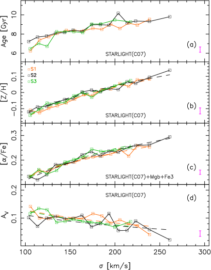
Figure 16: Same as Fig. 15 but for satellite rather than central ETGs.

The main result regarding the dependence with environment is that the stellar population content of central ETGs depends significantly on the mass of the halo where these galaxies reside. Central ETGs in groups, with “high” M_h(sample C2; see red curves in Figures 3 and Fig. 15), have younger ages, with $\delta(Age)\sim-1$ Gyr, higher metallicities, $\delta([Z/H])\sim 0.02$ dex, lower [$\alpha$/Fe], $\delta$[$\alpha$/Fe]$\sim-0.025$ dex, and higher extinction, $\delta$$\rm A_{V}$$\sim 0.035$ mag, than central ETGs with the same velocity dispersion, residing in lower mass halos (sample C1; see blue curves in the Fig. 4 and Fig. 16). This result is confirmed when using $\alpha$-MILES models (Fig. 15), from the analysis of line strengths (Sec. 4.2), or following an independent methodology that does not rely on stacked spectra (Gallazzi et al., in prep, see Appendix B). The environmental dependence of the age is detected throughout the whole range of velocity dispersion. Regarding metallicity, when using solar-scaled MILES models, the difference is present at all values of $\sigma$, except for two bins with $\sigma\sim 220$  km s^-1, whereas this trend is extended to all values of velocity dispersion when using the $\alpha$-MILES models (see panel b of Fig. 15).

–

In contrast, the stellar populations of satellite ETGs (Fig. 4) lack any significant difference with respect to environment, except for galaxies with low velocity dispersion ($\sigma<130$  km s^-1), where ETGs in the outskirts of groups (sample S3; see green curves in Fig. 4) have $\sim$1.5 Gyr younger ages, higher [$\alpha$/Fe] ($\sim+0.02$ dex when averaging over all three bins with $\sigma<130$  km s^-1), and higher $\rm A_{V}$  than satellites with high halo mass (i.e. those residing in galaxy “clusters”; see Sec. 2.2). Regarding the $Age$ parameter, satellites in lower mass halos (sample S1; see orange curves in the Figures) seem to lie in between the trends found for satellite ETGs in the outskirts of groups and those in more massive halos . These results are confirmed when using $\alpha$-MILES models (Fig. 16), as well as from the analysis of line strengths (Sec. 4.2).

–

Comparing the trends of Fig. 3 with those of Fig. 4, we see that satellite ETGs have a shallower $Age$–$\sigma$ relationship than central ETGs. For samples S1, S2, and S3, $Age$ is essentially constant for $\sigma>140$  km s^-1. In contrast, the $Age$ parameter keeps increasing up to $\sigma\sim 165$ km s^-1 ($\sim 185$  km s^-1) in centrals at low (high) M_h. For $\sigma<200$  km s^-1, satellites are always older, regardless of their environment, than groups’ centrals (sample C1). In other words, “downsizing” appears to be more pronounced in central ETGs than in satellites (see Sec. 6.1). The internal extinction vs. $\sigma$ trends are also steeper in the subsamples involving central ETGs (see the slope values in col. 4 of Tab. 4).

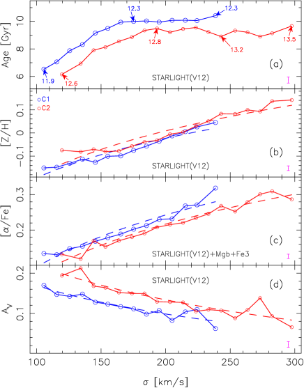
Figure 3: The trends of stellar population properties, $Age$ (a), metallicity (b), [$\alpha$/Fe] (c), and internal reddening (d), are shown as a function of velocity dispersion for central ETGs residing in low- (blue) and high- (red) mass halos. The two subsamples defined with respect to environment are shown with different colours as labelled in the top–left of panel (b). The magenta error bars in the lower–right corner of each panel show the maximum measurement uncertainty on stellar population parameters (i.e. the maximum value of the uncertainty among all data-points). The dark-grey labels in each panel refer to the method used to estimate the corresponding stellar population property. $Age$, metallicity, and extinction are estimated with STARLIGHT, while [$\alpha$/Fe] is obtained, at fixed age, from Mg and Fe spectral indices (see the text). In panel (a) the average $\log($M${}_{\rm h}/$M${}_{\odot})$ for specific bins of velocity dispersion is indicated.

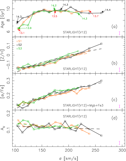
Figure 4: Same as Fig. 3 but for satellite rather than central ETGs.

4.2 Trends of line strengths with velocity dispersion

To further investigate the robustness of our results, we analyse the line strengths of spectral features sensitive to age and metallicity in the stacked spectra. We consider the age-sensitive Balmer lines $\rm H\beta_{o}$  and $\rm H\gamma_{F}$ , and the total metallicity indicator $\rm[MgFe]^{\prime}$. $\rm H\beta_{o}$  is a modified $\rm H\beta$  index, optimised to minimise the age-metallicity degeneracy (Cervantes & Vazdekis, 2009). Both $\rm H\beta$  and $\rm H\gamma_{F}$  are believed to be insensitive to [$\alpha$/Fe], in contrast to higher-order Balmer lines (Thomas, Maraston, Korn, 2004). In order to correct the $\rm H\beta_{o}$ line for nebular emission, we applied the same approach as in Paper VIII, where the $\rm H\beta$ spectral region (from $4000$ to $4950$ Å) is fitted with 2SSP (MILES) models (including a low-order multiplicative polynomial in the fit), excluding the H$\beta$ line (from $4857$ to $4865$ Å) from the fit. The variation of the $\rm H\beta_{o}$  index between a given observed spectrum and its best-fit model gives the emission correction. The uncertainty on the emission correction is estimated as half of the maximum variation in the emission correction when changing the order of the multiplicative polynomial (from $3^{\rm rd}$ to $6^{\rm th}$ order). We point out that the same emission correction approach is applied to all stacks. No emission correction is applied to $\rm H\gamma_{F}$, as higher-order Balmer lines are negligibly affected by nebular contamination in ETG spectra. The total metallicity estimator $\rm[MgFe]^{\prime}$  is a modified version of the González (1993) $\rm[MgFe]$ spectral index that removes its residual dependence on [$\alpha$/Fe]  (Thomas, Maraston, Bender, 2003). Hence, the analysis of $\rm H\beta_{o}$, $\rm H\gamma_{F}$, and $\rm[MgFe]^{\prime}$ is virtually free from any degeneracy among age/metallicity and either [$\alpha$/Fe] or $\rm A_{V}$, providing complementary information to that obtained with spectral fitting. Since we have only three spectral indices we do not attempt any fitting of line strengths with models having varying age and metallicity, but compare instead the trends for different samples of ETGs in a qualitative manner.

Figs. 5 and. 6 plot the age-sensitive indicators $\rm H\beta_{o}$ and $\rm H\gamma_{F}$ as a function of the metallicity estimator $\rm[MgFe]^{\prime}$, for central and satellite ETGs, respectively. Notice that the relatively large error bars on $\rm H\beta_{o}$  mainly reflect the uncertainties from the emission correction, rather than from the $S/N$ ratio of the spectra. The information contained in the two Figures can be compared with that of the age and metallicity trends in panels (a) and (b) of Figs. 3 and 4, respectively. Colours and symbol types are the same in Fig. 5 (Fig. 6) and Fig. 3 (Fig. 4). Labels and arrows in the Figures allow one to examine the trends in the line strengths at fixed $\sigma$. Fig. 5 shows that central ETGs in groups (“high” M_h) follow a different sequence than those with low M_h, providing further support to the main result of the present work, i.e. the significant dependence of stellar population properties of central ETGs on environment. When looking at line strengths for fixed $\sigma$, one can see that at low $\sigma$ (see the two bins with $\sim 120$ and $\sim 145$  km s^-1, respectively) the shift between the two sequences of central ETGs (red and blue curves) is mainly due to a “vertical” offset, caused by high M_h  centrals having stronger Balmer lines, i.e. younger ages and slightly higher metallicity, than those at low M_h. At high $\sigma$, due to the decreasing sensitivity of Balmer lines to a variation of age for old stellar populations, the origin of the difference between the two sequences becomes less clear. These results are qualitatively consistent with the offset between red and blue curves in panel (a) of Fig. 3. Fig. 6 shows that all satellite samples exhibit similar trends in the $\rm H\beta_{o}$– $\rm[MgFe]^{\prime}$ and $\rm H\gamma_{F}$– $\rm[MgFe]^{\prime}$  diagrams, with a tendency for satellites in the group outskirts (green curves) to have younger ages, at low $\sigma$, with respect to the other satellite samples, consistent with the results from spectral fitting (Fig. 4).

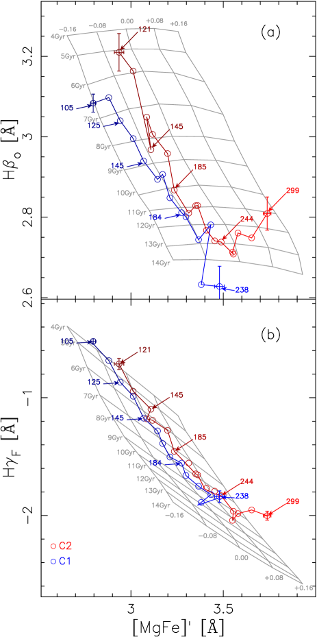
Figure 5: The EWs of the Balmer line strengths $\rm H\beta_{o}$  (top) and $\rm H\gamma_{F}$ (bottom) , are plotted as a function of the total metallicity indicator $\rm[MgFe]^{\prime}$, for the same environment-segregated samples as in Fig. 3, i.e. central ETGs at low and high halo-mass (blue and red colours, respectively). For each sample the colour of the symbols and the lines becomes lighter with increasing $\sigma$. Error bars (at the 1 sigma level) are shown only at the lowest and highest $\sigma$ bins, for each sample. Arrows are used to indicate the $\sigma$ value of some bins (in  km s^-1), in order to allow for a comparison of the different curves at fixed velocity dispersion. The grey grid shows the effect of varying age and metallicity of the MILES SSP models with a Kroupa IMF. The age is varied from 4 (top) to 14 Gyr (bottom) in steps of 1 Gyr, whereas the metallicity ranges from $[Z/H]$$=-0.16$ (left) to $+0.16$ (right), in steps of $0.08$ dex.

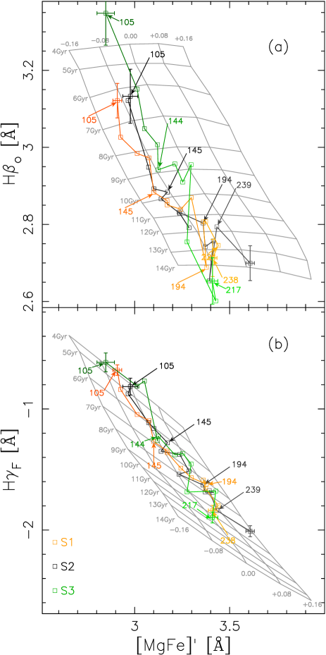
Figure 6: Same as Fig. 5 but for satellite rather than central ETGs. The Figure shows the same environment-segregated samples as in Fig. 4.

5 Possible systematic effects

We present in this section a battery of tests proving that the results shown in Figs. 3 and 4 are not affected by systematics. These tests can be summarized as follows:

Correlated uncertainties -

An important issue for any study of stellar populations is the effect of degeneracies among the various properties that define a population. In particular, underestimating the age of a stellar population can be balanced by an increase of its estimated metallicity (Worthey, 1994) and dust content. We notice that the results of the present work, and in particular the difference between the trends of samples C1 and C2, are not affected by this degeneracy. Firstly, there is no reason why such a degeneracy should affect only the samples of centrals, and not that of satellite ETGs. More importantly, differences between samples C1 and C2 are confirmed by an independent analysis of line strengths (see below, and Appendix B), which is unaffected by the age–dust degeneracy, and relatively unaffected by the age–metallicity degeneracy (when relying on the $\rm H\beta_{o}$ age indicator, see Sec. 4.2). In App. C, we also show that measurement errors tend to shift the stellar population properties of samples C1 and C2 along parallel loci in the space of $Age$, $[Z/H]$, and $\rm A_{V}$. Therefore, the differences between the blue and red curves in each panel of Fig. 3 are not artefacts from stellar population degeneracies or caused by a particular marginalisation of the uncertainties along a specific direction in the parameter space explored.

Uncertainties on M_h -

We have also verified that the stellar population trends for central ETGs are not affected by the uncertainties on halo mass estimates. To this effect, we have repeated the analysis by re-defining samples C1 and C2 with different mass thresholds of $\log($M${}_{\rm h,1}/$M${}_{\odot})$$<12.3$ and $\log($M${}_{\rm h,2}/$M${}_{\odot})$$>12.7$, respectively, rather than using a single separation value of $\log($M${}_{\rm h}/$M${}_{\odot})$$=12.5$ (see Sec. 2.2). The difference between M_h,1 and M_h,2 is roughly twice the group mass uncertainty estimated by Y07 for $\log($M${}_{\rm h}/$M${}_{\odot})$$\sim 12$ (see Sec. 2.2). We found median differences of $\delta(Age)\sim-1.1$ Gyr, $\delta([Z/H])\sim 0.02$ dex, $\delta$[$\alpha$/Fe]$\sim-0.038$ dex, and $\delta$$\rm A_{V}$$\sim 0.048$ mag, between group and isolated centrals, consistent with Fig. 3.

S/N ratio of SDSS spectra -

Our reference stacks are obtained by excluding spectra whose $S/N$ ratio is below the lowest quartile of the $S/N$ distribution of all ETG spectra within each $\sigma$ bin (see Sec. 2.1). We have repeated the analysis by removing this cut in $S/N$. The size of the sample increases from $N_{ETGs}=20,977$ to $28,356$. The fraction of ETGs excluded by the $S/N$ cut amounts to $f_{\rm S/N}\sim 28\%$, $12\%$, $27\%$, $32\%$, and $30\%$, for samples C1, C2, S1, S2, and S3, respectively. Notice that the lowest value of $f_{\rm S/N}$ corresponds to sample C2 as galaxies in the more massive halos are brighter (see below). Although $f_{\rm S/N}$ varies among different samples, the results of Figs. 3 and 4 turn out to be unaffected by the $S/N$ selection. This is shown in Figs. 7 and 8, where we compare the trends of stellar population parameters among stacked spectra obtained with (solid curves) and without (dot-dashed curves) the $S/N$ selection. Relative differences among samples (e.g. C1 and C2, as well as those among S1, S2, and S3 at lowest $\sigma$) are completely unaffected by the $S/N$ cut.

Trends for individual and stacked spectra -

As mentioned in Sec. 4.1 and shown in Appendix B, the trends of Figs. 3 and 4 are confirmed when using an independent methodology that relies on individual, rather than stacked, spectra, as well as a different set of stellar population models (BC03 rather than MILES), to infer the $Age$, $[Z/H]$, and [$\alpha$/Fe] parameters (Gallazzi et al., in prep). We have also derived $Age$, $[Z/H]$, [$\alpha$/Fe], and $\rm A_{V}$ from individual spectra with the same identical approach as for stacked spectra (Secs. 3.1 and 3.2). Fig. 9 compares the trends with $\sigma$ for central ETGs when using stacked spectra (solid curves, i.e. the same as in Fig. 3) and median-combining (dashed curves) the estimates from individual spectra. Although we have run STARLIGHT with the same setup, and in particular the same input basis of SSP models (see Sec. 3), for both stacked and individual spectra, some differences exist between the two approaches, as age and [$\alpha$/Fe] are systematically lower (by $\sim 2$ Gyr and $\sim 0.04$ dex, respectively), while $[Z/H]$ is systematically higher (by $\sim 0.04$ dex) for median values with respect to stacked spectra. The fact that the median ages from individual spectra are lower than the estimates from stacked spectra is likely due to the larger number  of young ($\;\buildrel<\over{\sim}\;$8–9 Gyr, typical for ETGs in our sample), relative to old (i.e. $\;\buildrel>\over{\sim}\;$8–9 Gyr), SSPs in the input basis provided to STARLIGHT. Because of that, at the relatively low-$S/N$ ratio of individual SDSS spectra, young SSPs get a non-zero weight more frequently than the old ones in the best-fitting STARLIGHT mixture, hence leading to lower age values (and thus higher $[Z/H]$, because of the age–metallicity degeneracy) when averaging over a given set of spectra. Nevertheless, as shown in Fig. 9, relative differences among samples still hold, regardless of the approach adopted.

Selection effects -

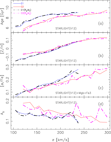
Figure 12: Comparison of median trends of stellar population properties for samples C1 and C2 (solid curves), with those (dot-dashed curves) for subsamples C1$($$\rm R_{\rm e}$;$\rm M_{\star}$$)$ and C2$($$\rm R_{\rm e}$;$\rm M_{\star}$$)$ (plotted as dot-dashed black and magenta curves also in Fig. 10). These subsamples are constructed from C1 and C2 to span the same range of stellar mass and galaxy size (see the text for details). Notice that the solid curves are the same as in Fig. 9 for reference.

Figs. 10 and 11 show the median trends (solid curves) of stellar mass, $\rm M_{\star}$, and effective radius, $\rm R_{\rm e}$, as a function of $\sigma$ for central and satellite ETGs, respectively, with dashed lines marking the 16th and 84th percentiles of the distributions. Stellar masses have been estimated from the available photometry (SDSS griz plus UKIDSS YJHK photometry) for each SPIDER ETG, as detailed in Paper V, while effective radii have been obtained by processing SDSS frames with the software 2DPHOT (see Paper I for details). While no significant difference is seen among the three samples of satellites, samples C1 and C2 differ significantly, with ETGs at high halo-mass having larger $\rm R_{\rm e}$ and $\rm M_{\star}$ than those at low M_h. This difference is because of the correlation between $\rm M_{\star}$ and M_h for centrals, and the mass–size relation of ETGs (see, e.g., Bernardi et al. 2014 and references therein). Since age is generally found to increase with galaxy mass (e.g. Gallazzi et al. 2006), and ETGs have shallow age gradients in their inner regions (La Barbera et al., 2012), any difference in $\rm R_{\rm e}$ and $\rm M_{\star}$ between C1 and C2 should not affect those presented in Fig. 3 (at least the age–$\sigma$ trends in panel a). To address this issue more explicitly, i.e. to test whether differences in the stellar population properties of centrals are affected by those in mass and radius, we select two subsamples of ETGs from C1 and C2, respectively, consisting of galaxies within the same range of $\rm M_{\star}$ and $\rm R_{\rm e}$ for both samples. In practice, we select C1 and C2 ETGs within the 16th and 84th percentiles of the $\rm M_{\star}$ and $\rm R_{\rm e}$ distributions for C1 (i.e. C1 and C2 galaxies that lie within the blue-dashed curves in both the upper and lower panels of Fig. 10). This selection produces two samples of $5,550$ (C1) and $795$ (C2) ETGs, whose median $\rm M_{\star}$ and $\rm R_{\rm e}$ differ by less than 0.1 dex for all $\sigma$ bins (see black and magenta dot-dashed curves in Fig. 10). Hereafter, we refer to these subsamples as C1$($$\rm R_{\rm e}$;$\rm M_{\star}$$)$ and C2$($$\rm R_{\rm e}$;$\rm M_{\star}$$)$, respectively. Fig. 12 compares the median trends of stellar population properties for C1 and C2 (solid curves; the same as in Fig. 9) to those for C1$($$\rm R_{\rm e}$;$\rm M_{\star}$$)$ and C2$($$\rm R_{\rm e}$;$\rm M_{\star}$$)$ (dot-dashed curves). Remarkably, although the $\rm M_{\star}$ and $\rm R_{\rm e}$ selection reduces the size of the parent samples C1 and C2, the trends of stellar population properties do not change significantly, confirming the robustness of our result, i.e. that central ETGs at high M_h have younger ages, lower $\alpha$-enhancement, higher extinction (and slightly higher $[Z/H]$) than those residing in lower mass halos.

Aperture effects -

SDSS spectra are observed within a fixed aperture of 3^′′ diameter. Because of the existence of radial gradients of stellar population properties in ETGs, the use of a fixed aperture might bias stellar population trends with $\sigma$ and environment. Indeed, as found in Paper II (see also Scodeggio et al. 1998), trends of age and metallicity with galaxy mass can be significantly shallower when these parameters are estimated for a whole galaxy, rather than its central regions. For the purpose of the present work, we assess whether aperture effects can introduce differences among samples of central and satellite ETGs. Tab. 3 reports the median fibre diameter, $\rm D_{fiber}$, and the lowest and highest 16th percentiles of the $\rm D_{fiber}$ distributions, for the samples of centrals and satellites. The values of $\rm D_{fiber}$ have been computed after rescaling, for each galaxy, the fibre diameter to physical projected distances (i.e. in kpc units), using SDSS spectroscopic redshifts. The median value of $\rm D_{fiber}$ is consistent among samples, amounting to $\sim 4$ kpc in general. Comparing the fibre projected physical distance to effective radii, we find for satellite ETGs that the typical $\rm R_{\rm e}$  is $\sim 4$ kpc in all samples (S1, S2, and S3; see Fig. 11), meaning that the SDSS fibre samples the same galactocentric distance of about $\rm R_{\rm e}$/2 for all satellites. Hence, aperture effects do not introduce a bias in the comparison of trends for S1, S2, and S3 in Fig. 4. For central ETGs, we notice that while the median $\rm D_{fiber}$  is the same for C1 and C2, ETGs in C2 have larger $\rm R_{\rm e}$ (by $\sim 0.3$ dex, i.e. a factor of two in linear units) than those in C1 (Fig. 10). Hence, the SDSS fibre samples a more central region for C2 (i.e. a galactocentric distance of $\sim$$\rm R_{\rm e}$$/4$) than for C1 (i.e. a galactocentric distance of $\sim$$\rm R_{\rm e}$$/2$). Since ETGs have negative metallicity gradients (i.e. higher metallicity in the centre than in the outskirts; e.g. Peletier et al. 1990) , one could expect that aperture effects may be responsible for the difference in $[Z/H]$  between C1 and C2 (panel b of Fig. 3). However, this is not necessarily the case, as the seeing, whose typical extent for SDSS data is FWHM$\sim 1.4^{\prime\prime}$ in the r band, tends to wash out stellar population gradients over a spatial scale of a few arcsec (mapping into a scale of $\sim$$\rm R_{\rm e}$$/2$ in C1). Tab. 3 shows that the subsamples C1$($$\rm R_{\rm e}$;$\rm M_{\star}$$)$ and C2$($$\rm R_{\rm e}$;$\rm M_{\star}$$)$, selected to span the same range of $\rm R_{\rm e}$ and $\rm M_{\star}$ (see above), have the same range of $\rm D_{fiber}$ (i.e. the same median and percentile values), i.e. the SDSS fibre spans the same galactocentric distance, in units of $\rm R_{\rm e}$, for both C1$($$\rm R_{\rm e}$;$\rm M_{\star}$$)$ and C2$($$\rm R_{\rm e}$;$\rm M_{\star}$$)$. Since stellar population differences between C1$($$\rm R_{\rm e}$;$\rm M_{\star}$$)$ and C2$($$\rm R_{\rm e}$;$\rm M_{\star}$$)$ are the same as those between C1 and C2, we conclude that aperture effects do not affect the results of our work.

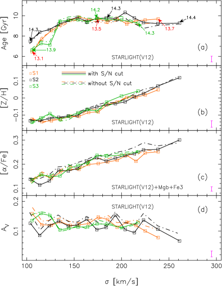
Figure 8: Same as Fig. 7 but for the samples of satellite ETGs. Solid curves and labels are the same as in Fig. 4.

Table 3: Median values, among different $\sigma$ bins, of the 16th (col. 2), 50th (i.e. the median; col. 3), and 84th (col.4) percentiles of (3^′′) SDSS-fibre diameter values, rescaled to kpc according to galaxy spectroscopic redshifts, for different samples of ETGs. Values in parentheses are standard deviations (among $\sigma$ bins). Samples C1($\rm R_{\rm e}$; $\rm M_{\star}$) and C2($\rm R_{\rm e}$; $\rm M_{\star}$) are obtained from C1 and C2 by selecting ETGs in the same range of $\rm M_{\star}$ and $\rm R_{\rm e}$(see the text).

SAMPLE	fibre diameter (kpc)
	16th percentile	median	84th percentile
(1)	(2)	(3)	(4)
C1	$3.48(0.14)$	$4.13(0.20)$	$4.82(0.16)$
C2	$3.50(0.15)$	$4.23(0.26)$	$4.93(0.19)$
S1	$3.46(0.11)$	$4.14(0.15)$	$4.83(0.07)$
S2	$3.48(0.11)$	$4.10(0.14)$	$4.78(0.08)$
S3	$3.44(0.14)$	$4.05(0.13)$	$4.72(0.08)$
C1($\rm R_{\rm e}$; $\rm M_{\star}$)	$3.49(0.07)$	$4.10(0.15)$	$4.85(0.15)$
C2($\rm R_{\rm e}$; $\rm M_{\star}$)	$3.42(0.20)$	$4.05(0.28)$	$4.92(0.23)$

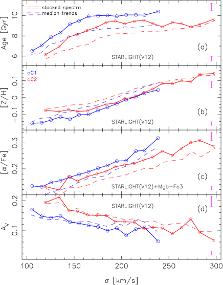
Figure 9: Comparison of the trends of stellar population properties of central ETGs obtained from our stacked spectra (solid curves) and by taking median values of the estimates for individual SDSS spectra in each velocity dispersion bin (dashed curves). Notice that solid curves and the magenta error bars in the lower–right of each panel are the same as in Fig. 3. Magenta error bars are maximum uncertainties (among bins and samples) for median-combined (dashed curves) trends.

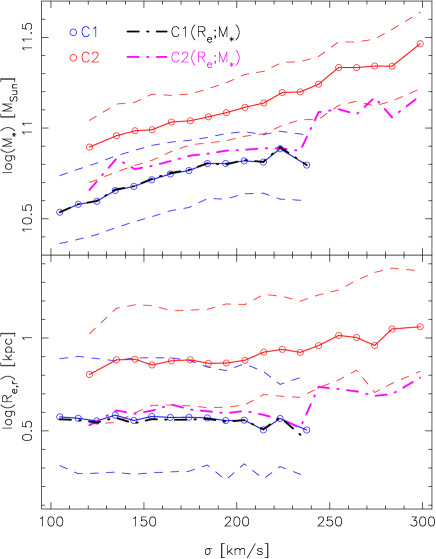
Figure 10: Trends of logarithmic stellar mass (top) and (r-band) effective radius (bottom) as a function of velocity dispersion for central ETGs residing in low-(blue) and high-(red) mass halos (i.e. samples C1 and C2, respectively; see top–left labels). Solid curves are median trends, while dashed curves mark the 16th-84th percentiles of the distributions for each $\sigma$ bin. Because of the $\rm M_{\star}$–halo mass correlation for centrals and the mass-size relation of ETGs, galaxies in sample C2 tend to be more massive and larger than those in C1. Black and magenta dot-dashed curves show the trends for the subsamples C1$($$\rm R_{\rm e}$;$\rm M_{\star}$$)$ and C2$($$\rm R_{\rm e}$;$\rm M_{\star}$$)$, obtained by selecting ETGs with the same range of $\rm R_{\rm e}$ and $\rm M_{\star}$ from samples C1 and C2, respectively.

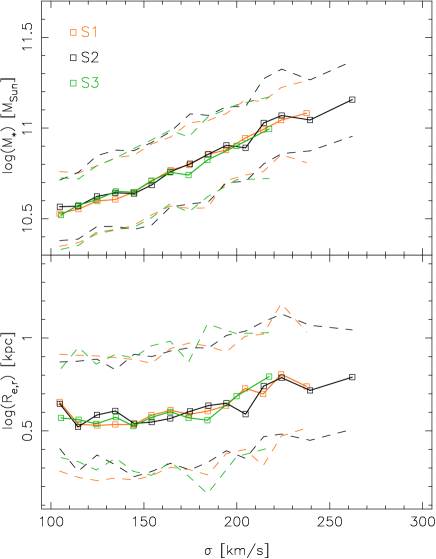
Figure 11: Same as Fig. 10 but for the three samples of satellite ETGs. Notice that the distributions of stellar mass and effective radius are now independent of the environment.

6 Comparison to previous works

6.1 Trends with velocity dispersion

Since the slopes of $[Z/H]$ and [$\alpha$/Fe] with $\sigma$ are independent of environment (Tab. 4), it is useful to derive the average slopes among all five samples of ETGs, i.e.

$$\beta_{Z\!/\!H}=\frac{\delta([Z/H])}{\delta(\log\sigma)}=0.58\pm 0.05,$$ (2)

and

$$\beta_{\alpha\!/\!{\rm Fe}}=\frac{\delta([\alpha/{\rm Fe}])}{\delta(\log\sigma)}=0.42\pm 0.06.$$ (3)

These values can be compared with those obtained from past studies (Trager et al., 2000; Bernardi et al., 2003; Thomas et al., 2005; Smith et al., 2007; Zhu, Blanton, Moustakas, 2010; Thomas et al., 2010; Harrison et al., 2011). As shown in Harrison et al. (2011, see their table 5), different studies found a wide range of values of $\beta_{Z\!/\!H}$ ($\beta_{\alpha\!/\!{\rm Fe}}$), from $\sim 0.18$ ($0.2$) to $\sim 0.79$ ($0.36$). This range of values is likely due to different methods used to derive stellar population parameters, as well as different selection criteria of the samples. Our values of $\beta_{Z\!/\!H}$  and $\beta_{\alpha\!/\!{\rm Fe}}$ overlap, within the uncertainties, with the range of values in the literature. In particular, despite the different methodology used to derive $[Z/H]$  and [$\alpha$/Fe], our values of $\beta_{Z\!/\!H}$  and $\beta_{\alpha\!/\!{\rm Fe}}$  are fairly consistent, at the 1.5 $\sigma$ level, with those recently obtained by Thomas et al. (2010), i.e. $\beta_{Z\!/\!H}$$=0.65\pm 0.02$ and $\beta_{\alpha\!/\!{\rm Fe}}$$=0.33\pm 0.01$, for morphological-selected samples of ETGs drawn from the SDSS. Regarding the $Age$ parameter, most studies agree, in particular at low $\sigma$, that age increases with velocity dispersion. This finding fits well with the downsizing picture of galaxy formation, where the typical mass of star forming galaxies is seen to shift towards higher values with look-back time (e.g. Cowie et al. 1996). We notice that the increasing trends of $Age$ and $[Z/H]$  with $\sigma$ also agree qualitatively with our previous work (Pasquali et al., 2010, PGF10), where we analysed the trends of such parameters with stellar mass (instead of velocity dispersion) for the whole population of galaxies (rather than selecting ETGs only, as in the present work), as well as with the trends as a function of stellar and dynamical mass found for ETGs (selected by the concentration of the light profile) in Gallazzi et al. (2006). We emphasise that although the trends presented in this work are consistent with previous works, our study allows us to explore for the first time how at fixed velocity dispersion, the stellar population parameters depend in a different way on halo mass for central and satellite ETGs.

Table 4: Slopes of the correlations between $[Z/H]$  (col. 2), [$\alpha$/Fe] (col. 3) and $\rm A_{V}$ (col. 4), vs. $\log\sigma$, for different samples of ETGs (col. 1; see Tab. 1). Errors are quoted at the 1 $\sigma$ level. Values in parentheses are those obtained with $\alpha$-enhanced (rather than “standard”) MILES models.

SAMPLE	$[Z/H]$ slope	[$\alpha$/Fe] slope	$\rm A_{V}$ slope
(1)	(2)	(3)	(4)
$\rm C1$	$0.57\pm 0.07(0.65\pm 0.03)$	$0.48\pm 0.06(0.49\pm 0.06)$	$-0.23\pm 0.03(-0.32\pm 0.03)$
$\rm C2$	$0.64\pm 0.07(0.66\pm 0.04)$	$0.47\pm 0.04(0.44\pm 0.04)$	$-0.29\pm 0.04(-0.34\pm 0.03)$
$\rm S1$	$0.54\pm 0.07(0.62\pm 0.05)$	$0.33\pm 0.03(0.33\pm 0.03)$	$-0.10\pm 0.05(-0.15\pm 0.05)$
$\rm S2$	$0.60\pm 0.06(0.59\pm 0.04)$	$0.43\pm 0.03(0.41\pm 0.03)$	$-0.04\pm 0.06(-0.12\pm 0.05)$
$\rm S3$	$0.53\pm 0.08(0.61\pm 0.05)$	$0.40\pm 0.03(0.41\pm 0.04)$	$-0.08\pm 0.07(-0.16\pm 0.04)$

Table 5: Intercepts of the correlations between $[Z/H]$  (col. 2), [$\alpha$/Fe] (col. 3) and $\rm A_{V}$ (col. 4), vs. $\log\sigma$, for different samples of ETGs (col. 1; see Tab. 1). The intercepts are computed at a reference velocity dispersion of $200$  km s^-1. Errors are quoted at the 1 $\sigma$ level. Values in parentheses are those obtained with $\alpha$-enhanced (rather than “standard”) MILES models.

SAMPLE	$[Z/H]$ intercept	[$\alpha$/Fe] intercept	$\rm A_{V}$ intercept
(1)	(2)	(3)	(4)
$\rm C1$	$-0.023\pm 0.006(0.015\pm 0.003)$	$0.243\pm 0.006(0.247\pm 0.006)$	$0.099\pm 0.005(0.059\pm 0.005)$
$\rm C2$	$0.009\pm 0.008(0.046\pm 0.003)$	$0.217\pm 0.003(0.224\pm 0.003)$	$0.134\pm 0.003(0.097\pm 0.003)$
$\rm S1$	$-0.019\pm 0.006(0.032\pm 0.004)$	$0.222\pm 0.003(0.229\pm 0.004)$	$0.115\pm 0.006(0.083\pm 0.006)$
$\rm S2$	$-0.003\pm 0.006(0.042\pm 0.005)$	$0.237\pm 0.003(0.241\pm 0.003)$	$0.111\pm 0.007(0.073\pm 0.009)$
$\rm S3$	$-0.009\pm 0.012(0.039\pm 0.008)$	$0.242\pm 0.005(0.246\pm 0.006)$	$0.115\pm 0.007(0.076\pm 0.006)$

6.2 Trends with environment

As reported in Sec. 1, most of the previous studies have analysed stellar population properties of ETGs as a function of “local” environment, characterised either through local galaxy density or by splitting ETGs into field and cluster samples (e.g. Bernardi et al. 2003, 2006; Thomas et al. 2005, 2010; Annibali et al. 2007; Clemens et al. 2009; Zhu, Blanton, Moustakas 2010; Cooper et al. 2010). A general consensus has emerged that, at fixed galaxy mass, either the whole population or some fraction of ETGs in low-density regions host younger stellar populations than those in dense regions (i.e. cluster cores). This difference is found to increase towards lower mass galaxies. In order to compare our findings with these works, we use the definition of ETG environment as in  La Barbera et al. (2010b, hereafter Paper III). Using an updated FoF group catalogue created as in Berlind et al. (2006) (the difference between the two being in the area used, i.e. SDSS/DR7 rather than DR3), in Paper III we classified SPIDER ETGs into group members, field galaxies (i.e. objects with no group membership assigned, and those far from any FoF group), and un-classified objects (mostly galaxies residing in poor groups and/or in the group “borders”, see Paper III for details). These three classes constitute 46%, 33%, and 21% of the entire SPIDER sample, respectively.

We note that the present study relies on a different group catalogue than that used in Paper III (i.e. the Yang et al., rather than Berlind et al., catalogue). Although a detailed comparison of different group catalogues is certainly beyond the scope of the present work, it is instructive to analyse the composition of the five samples of central and satellite ETGs in terms of the environment as defined in Paper III. Tab. 6 reports, for each sample, the fraction of field, group, and un-classified objects. As expected, the three samples of satellites (S1, S2, and S3) only include a negligible fraction of field galaxies, especially sample S2, i.e. galaxies residing in the central regions of massive groups (“clusters”), where no galaxy is classified as “field” according to Paper III. The Table also reveals that the population of centrals is much more heterogeneous, including a significant contribution ($>30$%) from field galaxies, in both samples C1 and C2 (i.e. regardless of halo mass), with a larger fraction ($>40$%; as it might be expected) for low-M_h  centrals. Despite this heterogeneity, as shown in Figs. 3 and 5, low- and high-mass centrals show remarkably different stellar population properties, reinforcing the conclusion that these differences are driven by the “global” environment (i.e. the halo mass) where galaxies reside.

To further analyze this aspect, we have constructed stacked spectra for two subsamples of central ETGs, consisting of (i) C1 centrals classified as field galaxies according to Paper III ($N_{ETGs}=4,380$), and (ii) C2 centrals classified as group galaxies from Paper III ($N_{ETGs}=2,349$). Fig. 13 compares the trends of stellar population properties with $\sigma$ for these subsamples with those for C1 and C2. While for C1 there is no significant change when selecting only “field” galaxies, selecting only C2 ETGs classified as “group” from Paper III produces some changes, in that (i) the difference in metallicity between C1 and C2 tends to disappear (see blue and red dashed curves in panel b of Fig. 13), and (ii) at low $\sigma$ ($\lower 2.15277pt\hbox{$\;\buildrel<\over{\sim}\;$}150$  km s^-1) the difference in age, [$\alpha$/Fe], and $\rm A_{V}$ becomes smaller than that between the whole samples of C1 and C2 ETGs. This test indicates that the dependence of stellar population properties on M_h holds up against a different definition of environment. The amplitude of the differences in stellar population properties between isolated and group ETGs is more significant when we add, to the C2 “group” galaxies of Paper III, those C2 centrals labelled “field” or “unclassified” in the same paper, likely residing in low-multiplicity groups, that the virial analysis of Paper III has not been able to measure.

Since our samples of satellites mostly consist of group galaxies, we can compare our findings, in Figs. 4 and 6, with those of previous studies contrasting the properties of ETGs as a function of local galaxy density. Indeed, the only environmental effect we detect for samples S1, S2, and S3, is that at low-$\sigma$, ETGs at large group-centric projected distances (sample S3) tend to have younger stellar populations than satellites in the central regions. This is consistent with Rogers et al. (2010), and the general finding that low-mass ETGs residing in low-density environments have younger stellar populations than those at high density. On the other hand, Bernardi et al. (2009) found that BCGs in groups are $\sim$0.5–1 Gyr older than their satellites (see also Pasquali et al. 2010). We notice that this result is not inconsistent with our findings as (i) we are not comparing the properties of satellites with their own centrals (samples C1 and C2 have different M_h  than samples S1, S2, and S3), but, rather, the two populations individually as a whole; and (ii) we are analyzing only ETGs rather than galaxies of all morphological types.

Regarding metallicity, we also find evidence that low-$\sigma$ ETGs in sample S3 (i.e. galaxies in “low-density” regions) have slightly higher $[Z/H]$ than satellites in the cluster cores (samples S1 and S2). This is consistently seen in the $\rm H\beta_{o}$–$\rm[MgFe]^{\prime}$ diagram (Fig. 6), where the trend for sample S3 (green curve) is shifted rightwards (i.e. towards higher $[Z/H]$) with respect to the trends for samples S1 and S2. This finding is consistent with previous studies (Thomas et al., 2005; de La Rosa et al., 2007; Clemens et al., 2009; Zhu, Blanton, Moustakas, 2010), as well as our inference from the environmental dependence of the Fundamental Plane relation of ETGs (Paper III). One should notice that some studies did not detect any environmental dependence of metallicity (e.g. Berlind et al. 2006; Annibali et al. 2007; Harrison et al. 2011), while others (Gallazzi et al., 2006) found ETGs in low-density environments to be less metal-rich than those at high density. These discrepancies likely arise both because of different definitions of environment, and because of the intrinsically small differences found in the stellar population properties among different environments.

Our new results can also be compared with those of PGF10, where low-mass satellites, in low-mass halos, were found to feature younger ages than those at increasing M_h. PGF10 interpreted the age trend as a result of satellites in today more, relative to less, massive halos having been accreted at earlier epochs. As shown in Fig. 4, comparing the low-$\sigma$ behaviour of samples S1 and S2, our results are consistent with this finding.

Table 6: Percentage of galaxies in each sample of ETGs (col. 1), classified as field and group systems, as well as unclassified objects, according to Paper III (cols. 2,  3, and 4, respectively).

sample	field	group	un-classified
(1)	(2)	(3)	(4)
C1	42%	27%	31%
C2	32%	47%	21%
S1	12%	62%	26%
S2	0%	84%	16%
S3	3%	78%	19%

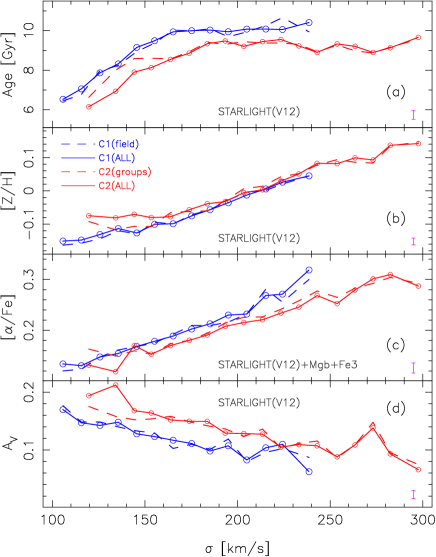
Figure 13: Trends of stellar population properties for stacked spectra of low-M_h centrals (C1) classified as “field” galaxies, and high-M_h centrals (C2) classified as “group” galaxies according to Paper III (based on the group catalogue of Berlind et al., 2006). Solid curves show the trends for the original samples of centrals, C1 and C2, used in this paper, i.e. as in Fig. 3.

7 Summary and Discussion

In the present work, we have studied how the stellar populations of ETGs depend on the “global” environment, characterised by the mass of the host halo. Since a key driver of the formation history of ETGs is the central velocity dispersion ($\sigma$, a “local” quantity mainly dependent on the evolution of the gravitational potential of the galaxy), we perform the comparisons regarding environment at fixed $\sigma$. We have performed a stellar population study of central and satellite ETGs, using 72 stacked SDSS spectra, covering a wide range in velocity dispersion: $100\!<\!\sigma\!<\!310$  km s^-1. The satellite sample is split into three subsamples, namely galaxies residing in the central regions ($<0.5\,R_{200}$) of “groups” (with halo mass $\log($M${}_{\rm h}/$M${}_{\odot})$$<\!14$) and “clusters” ($\log($M${}_{\rm h}/$M${}_{\odot})$$\geq 14$), respectively, and those residing in the outskirts ($\geq 0.5\,R_{200}$) of all groups/clusters (regardless of M_h). Central ETGs are binned into “isolated” systems ($\log($M${}_{\rm h}/$M${}_{\odot})$$<\!12.5$) and those residing in galaxy “groups” ($\log($M${}_{\rm h}/$M${}_{\odot})$$\geq\!12.5$). Our results are summarised as follows:

Global trends:

The stellar age, metallicity ($[Z/H]$), and [$\alpha$/Fe]  increase with velocity dispersion, regardless of environment. The slopes of the $[Z/H]$ and [$\alpha$/Fe] – $\sigma$ relations are consistent with previous studies (e.g. Trager et al. 2000; Bernardi et al. 2003; Thomas et al. 2005; Smith et al. 2007; Zhu, Blanton, Moustakas 2010; Thomas et al. 2010; Harrison et al. 2011). The age increases with $\sigma$ in low velocity dispersion systems ($\sigma<150$–$200$  km s^-1), whereas at higher velocity dispersion, it either remains constant or increases with $\sigma$, depending on the method used to derive the stellar population properties. ETGs at high $\sigma$ tend to have lower internal extinction than those at low $\sigma$. This trend is more significant in centrals than satellites.

Centrals:

The stellar population properties of central ETGs depend significantly on global environment. At fixed velocity dispersion, the centrals of galaxy groups have younger ages (at all values of $\sigma$), higher metallicites (especially at low $\sigma$), and lower [$\alpha$/Fe] than “isolated” centrals (i.e. those in lower mass halos).

Satellites:

In contrast to the centrals, no significant environmental dependence of stellar population properties is found in satellite ETGs, except for systems at the lowest velocity dispersions ($\sigma\!<\!130$  km s^-1), where satellites residing either in low-mass halos or in the outskirts of the more massive groups, seem to have younger ages than satellite ETGs residing in massive halos. These results are consistent with those of PGF10. In particular, the fact that, at low $\sigma$, satellites in low-mass halos have younger ages than those with high M_h can be explained by a later infall into the host halo, followed by quenching of their star-formation by environmental processes (e.g. strangulation).

The new main result of the present work is the dependence of stellar population properties of central ETGs on environment. What causes younger ages in the central ETGs of more massive halos? Since we analyse stacked spectra, these young ages may arise either because of a more prolonged star-formation in the average population of high-M_h galaxies, or because of a larger fraction of these galaxies with young stellar populations. For instance, Thomas et al. (2010) found that while the bulk of ETGs have $Age$, $[Z/H]$, and [$\alpha$/Fe]  vs. $\sigma$ trends independent of local environment (i.e. galaxy density), low-density regions feature a larger fraction of ETGs with stellar populations “re-juvenated” by a few Gyr. In Fig. 14, we present the cumulative stellar mass formation histories (SMFHs) for low- and high-M_h  centrals. The SMFHs are obtained from the STARLIGHT fits to the stacked spectra (see Sec. 3.1), as detailed in our previous works (de la Rosa et al., 2011; Trevisan et al., 2012). In the Figure, we average the results for stacks at low (i.e. $100\!<\!\sigma\!<\!180$  km s^-1) and high (i.e. $180\!<\!\sigma\!<\!250$  km s^-1) velocity dispersion. Centrals show smoothly declining SMFHs, with the bulk of the stellar mass formed at a lookback time $\lower 2.15277pt\hbox{$\;\buildrel>\over{\sim}\;$}6$ Gyr. For centrals in more massive groups (red curves in the Figure), the stellar component formed over a more extended time scale than in “isolated” (low halo mass) centrals (blue curves). This is fully consistent with the results shown in Fig. 3, which suggested that high-M_h centrals have younger ages, and lower [$\alpha$/Fe], than low-M_h  centrals. Since Fe mainly originates from the explosion of type Ia supernovæ, over a larger time scale than $\alpha$ elements (mostly produced in short-lived massive stars), a lower [$\alpha$/Fe] does in fact imply a more prolonged star formation history, consistent with Fig. 14. Quantitatively, we find that at high $\sigma$, centrals in low mass halos have [$\alpha$/Fe] $\sim 0.025$ dex higher (on average) than their counterparts in more massive halos (Fig. 3). Using eq. 2 of de la Rosa et al. (2011), such a difference translates into a half-mass formation time difference of $\sim 0.4$ Gyr, qualitatively consistent with the different shapes of the red and blue dashed curves in Fig. 14. For centrals with low $\sigma$, we also find a more prolonged SMFH in more massive halos (compare the red and blue solid curves), despite the fact that the difference in [$\alpha$/Fe] between low- and high- M_h samples is not as significant as at high $\sigma$ (Fig. 3). Fig. 14 also compares our SMFHs with those obtained by Pérez-González et al. (2008), from a sample of $28,000$ objects extended to all morphological types, at $0<z<4$. Because of the high star-formation efficiency (see, e.g., Ferreras et al., 2009; Trevisan et al., 2012), ETGs have shorter formation time scales than the overall population of galaxies, with the difference becoming smaller towards massive galaxies, as expected by the fact that most massive galaxies are early-type systems.

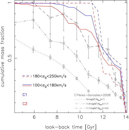
Figure 14: The stellar mass formation histories of the populations in central ETGs is shown as a function of look-back time. Notice that the plot is limited to epochs older than $\sim 4$ Gyr as the stellar mass fractions are identically equal to one below this value (i.e. negligible late star formation in our sample). The solid and dashed curves are the median trends for ETGs in low ($\sigma<180$  km s^-1) and high ($\sigma>180$  km s^-1) velocity dispersion bins, respectively. Blue and red colours correspond to the centrals in low- and high-mass halos, respectively, with the same colour coding as in Figs. 3 and 5. The figure shows that stellar populations in central ETGs in groups (high-mass halos) are formed at a lower pace than those in “isolation” (i.e. ETGs residing in low-mass halos), consistent with the results of our stellar population analysis (Fig. 3). Also, notice that star formation is more extended towards lower velocity dispersion. For comparison, we overplot the results from Pérez-González et al. (2008, grey) for three stellar mass bins, covering the entire stellar mass range of our sample (grey labels).

Within the current paradigm of galaxy formation, central galaxies can accrete gas from the hot-gas reservoir of their host halo (see, e.g., Croton et al., 2006). In the most massive halos, this hot-mode of star-formation is believed to be suppressed by feedback processes (e.g. AGN activity), in order to explain the old stellar ages and low-level of recent star-formation in massive galaxies at low redshift (De Lucia et al., 2006). The more prolonged SMFHs of centrals in high-mass halos might be due to a stronger accretion of hot gas from the surrounding halo. However, the gas should also cool down to sit into the central galaxy itself to form a disc (preserving its angular momentum). Since our sample is selected to minimise the contamination from systems with a disk component (see Sec. 2), we would expect this scenario to be ruled out. Instead, we interpret our findings as the result of gas-rich galaxy-galaxy interactions, between centrals residing in present-day groups, and the population of infalling satellites. These interactions are certainly more important in groups, than in “isolated” ellipticals (where, by definition, there are fewer satellites, see Fig. 1). In this framework, dissipative interactions should have been an essential ingredient of the mass accretion history of central ETGs in groups. In fact, major (minor) “dry” (dissipation-less) mergers are expected to increase (not change) the velocity dispersion (Hilz et al., 2012). Assuming that the trends for “isolated” centrals at low redshift are representative of those of the progenitors of central ETGs in more massive groups today, major dry mergers would lead to a horizontal shift (see Fig. 3) towards higher $\sigma$ of all stellar population trends regarding central ETGs. While the trends for $Age$, [$\alpha$/Fe], and $\rm A_{V}$  are consistent with this scenario, the trends for metallicity are not. On the other hand, simulations suggest that gas-rich interactions can produce a significant dilution of metallicity only during the first phases of the interaction, especially for intense levels of star-formation, after which enrichment becomes the dominant effect, so that metallicity is expected to be larger in the final system than in the progenitors (Montuori et al., 2010). This mechanism goes in the direction of increasing the metallicity of centrals in more massive halos, as observed in Fig. 3. Therefore, the results of this work point consistently to a picture whereby central ETGs in groups evolve through a higher number of gas-rich galaxy-galaxy interactions, resulting in slightly more extended star formation histories with respect to “isolated” ETGs – although the “local” physics, parameterised as central velocity dispersion, remains the main driver of star formation in ETGs, a result that is consistent with the properties of star forming galaxies as well (see, e.g., Wijesinghe et al., 2012).

It is also worth emphasising that the subtle but consistent differences found between the stellar populations in central and satellite ETGs confirm that a central/satellite split is the key property that allows us to understand in detail the effect of environment on galaxy formation.

Appendix A Running STARLIGHT with $\alpha$-enhanced SSPs

We test the effect of using solar-scaled models on the derived stellar population properties of ETGs by comparing our results with a preliminary set of $\alpha$-enhanced MILES (hereafter $\alpha$-MILES) SSP models constructed by Cervantes et. al. (2007), based on both empirical and theoretical stellar libraries. The empirical MILES library (Sánchez-Blazquez et al. 2006) contains spectra of stars in the solar neighbourhood, but mostly lacks bulge-stars, with non-solar abundance ratios. The $\alpha$-MILES models complement the empirical library, in the non-solar abundance regime, with the synthetic library of Coelho et al. (2007), consisting of high-resolution synthetic stellar spectra covering a wide range of stellar atmospheric parameters. The Coelho et al. (2007) library covers both solar and alpha-enhanced mixtures over a wide wavelength range, from $3000$Å to 1.4 $\mu$m, superseding previous versions of Barbuy et al. (2003), in the wavelength range $4600-5600$Å, and Zwitter, Castelli, Munari (2004), in the range $7653-8747$Å. The resulting $\alpha$-enhanced models consist of SEDs covering the same spectral range ($3525-7500$ Å), with the same spectral resolution ($2.3$Å), as the (nearly solar-scaled) MILES models used in this paper. As shown in Paper IV, the preliminary $\alpha$-enhanced models are more effective at describing the spectra of massive ETGs than the solar-scaled models, in particular concerning spectral features strongly sensitive to [$\alpha$/Fe], such as Mg lines. The $\alpha$-MILES models consist of $1,170$ SSPs, corresponding to: twenty-six ages from $1$ to $18$ Gyr; five metallicities from $[Z/H]$$=-1.28$ to $+0.2$, and nine value of [$\alpha$/Fe], from $-0.2$ to $+0.6$. With this set of models, we have run STARLIGHT on our stacked spectra, using a basis of $224$ $\alpha$-MILES SSPs (see Sec. 3.1), with 14 steps in age, from $1$ to $14$ Gyr, four steps in $[Z/H]$  ($-0.7$, $-0.4$, $0$, and $+0.2$), and four steps in [$\alpha$/Fe] ($0$, $0.2$, $0.4$, $0.6$). For each stack, we compute age and metallicity from $\alpha$-MILES best-fitting (STARLIGHT) results, as described in Sec. 3.1 (i.e. from Eq. 1). Notice that one could use the $\alpha$-MILES STARLIGHT results also to compute luminosity-weighted estimates of [$\alpha$/Fe]  (through Eq. 1). However, we prefer to rely on our solar-scale proxy $[Z_{\rm Mg}/Z_{\rm Fe}]$  (Sec. 3.2), obtained with solar-scaled single-SSP MILES models, as such SSP-equivalent [$\alpha$/Fe]  estimates can be related more directly to the star-formation time scale of ETGs (de la Rosa et al., 2011). Thus, we re-compute [$\alpha$/Fe] for each stacked spectrum using the same approach as in Sec. 3.2, but using luminosity-weighted ages from the $\alpha$-MILES STARLIGHT fits. Figs. 15 and 16 are the same as Figs. 3 and 4, respectively, but for stellar population parameters from $\alpha$-MILES (instead of solar-scaled MILES) STARLIGHT fits. In general, using $\alpha$-MILES leads to consistent results with respect to the MILES models, although the trends of $Age$ and $\rm A_{V}$  with $\sigma$ are steeper (see Secs. 4 and 6, respectively). In particular, the main results of the present work – regarding the environmental comparison of satellite and central ETGs – do not depend on the adopted stellar population models.

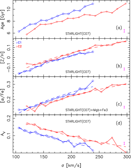
Figure 15: Same as Fig. 3 but deriving age and metallicity with $\alpha$-enhanced SSP models from Cervantes et al. (2007). Notice that [$\alpha$/Fe]  is estimated from the solar-scale proxy, $[Z_{\rm Mg}/Z_{\rm Fe}]$, as in Fig. 3, whereas age and metallicity are obtained by running STARLIGHT with $\alpha$-enhanced SSPs.

Appendix B Comparison with independent parameter estimates on individual galaxies

To further validate the robustness of our results, in particular against differences in stellar population modelling, we have compared them with those obtained from the analysis of a set of [$\alpha$/Fe]-independent absorption features of SDSS early-type galaxies by Gallazzi et al. (2006). In summary, the luminosity-weighted ages and stellar metallicities are derived via a Bayesian approach by comparing the strengths of $\rm D4000_{n}$, $\rm H\beta$, $\rm H\delta_{A}+H\gamma_{A}$, $\rm[Mg_{2}Fe]$, $\rm[MgFe]^{\prime}$ with a Monte Carlo library of star formation histories based on the Bruzual & Charlot (2003) population synthesis models. Estimates of element abundance ratio are based on the empirical estimator defined in Gallazzi et al. (2006), $\Delta$(Mgb/$\langle$Fe$\rangle$), which is the excess of the observed Mgb/$\langle$Fe$\rangle$ feature with respect to the solar-scaled model that best fits the above defined indices. This estimator is calibrated into [$\alpha$/Fe] using the predictions of Thomas, Maraston, Bender (2003) models (Gallazzi et al., in prep.). Note that in contrast to the rest of this paper, these parameters have been estimated for individual SDSS galaxies. For each central/satellite galaxy subsample and for each velocity dispersion bin, we take the median luminosity-weighted age, stellar metallicity and [$\alpha$/Fe]  of all the galaxies that contribute to the corresponding stacked spectrum. In analogy with Figs. 3 and 4, we show in Figs. 17 and 18 the results obtained for central galaxies and satellite galaxies, respectively. We notice a few differences with respect to Figs. 3 and 4. In particular stellar age does not show a flattening at high velocity dispersion but it keeps on increasing with $\sigma$, similar to Fig.  15 (derived from a preliminary set of $\alpha$-enhanced models). The slope is however shallower, reaching ages about 1 Gyr younger at high velocity dispersion than those shown in the previous figures. Despite these differences, the agreement with the results discussed in Figs. 3 and 4 is remarkable. In particular, we also confirm with these independent estimates, that i) central galaxies in larger halos are younger, more metal-rich and less $\alpha$-enhanced than central galaxies in lower-mass halos, and ii) the stellar populations of satellite early-type galaxies do no show any systematic trend with environment. This comparison also reassures us about the similarity of parameters obtained from our stacked spectra with respect to median parameter values of galaxies contributing to each bin as derived from individual spectra.

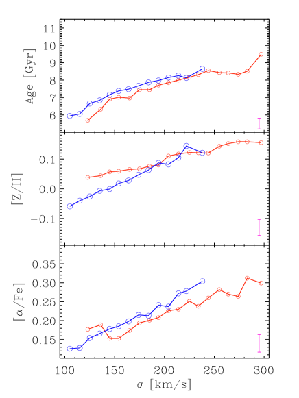
Figure 17: Luminosity-weighted age, stellar metallicity and [$\alpha$/Fe] as a function of velocity dispersion for central galaxies with $\log($M${}_{\rm h}/$M${}_{\odot})$$>12.5$ (red) and with $\log($M${}_{\rm h}/$M${}_{\odot})$$<12.5$ (blue). Ages and metallicities are derived as in Gallazzi et al. (2006) by comparing a set of absorption features with a Monte Carlo library of star formation histories based on the solar-scaled Bruzual & Charlot (2003) models. The [$\alpha$/Fe] estimates are derived from the empirical definition of Gallazzi et al. (2006), $\Delta({\rm Mgb}/\langle{\rm Fe}\rangle)$, calibrated with the Thomas, Maraston, Bender (2003) models. In all panels, magenta error bars in the lower-right corners correspond to the maximum values of $1$ sigma uncertainties on median values of stellar population properties among different data-points.

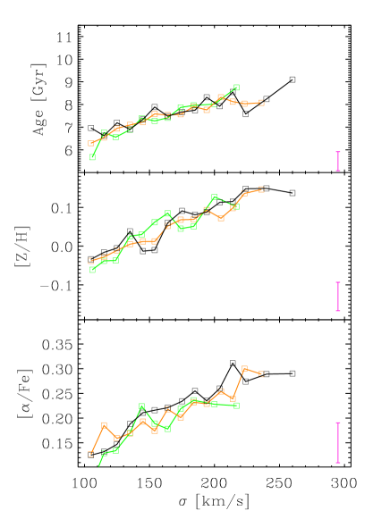
Figure 18: Same as Fig. 17, but for satellite galaxies (same colour-coding as in Fig. 3).

Appendix C Correlated uncertainties of stellar population parameters.

We illustrate the effect of correlated uncertainties on stellar population parameters by considering two stacked spectra from samples C1 and C2, respectively, both at a velocity dispersion in the range $\sigma\sim 200$–$210$  km s^-1. For each spectrum, we performed $1000$ iterations, where $Age$, $[Z/H]$, and $\rm A_{V}$  are re-measured with STARLIGHT on spectra where the flux values are randomly modified according to their uncertainties (see Sec. 3 for details). Fig. 19 shows the distribution of the measurements for both spectra, in the $Age$ vs. $[Z/H]$  and $Age$ vs. $\rm A_{V}$  diagrams, including the 1 and 2 $\sigma$ confidence levels. As expected, measurement errors tend to shift the fiducial values in the plots (filled circles) along anti-correlated directions of $Age$–$[Z/H]$  and $Age$–$\rm A_{V}$  (see dashed lines in the Figure). However, the directions of correlated errors, between C1 and C2 stacks, are almost parallel, i.e. the difference of $Age$, $[Z/H]$, and $\rm A_{V}$  between samples C1 and C2 do not arise because of correlated uncertainties. Would this have been the case, we would have measured much larger differences in metallicity with respect to those we measure in the $Age$ parameter, as this would be required to shift horizontally the red dot in the left panel of Fig. 19 towards the blue dashed curve. This result gives further support to the fact that the environmental differences detected in the present work, and in particular those for central ETGs, arise neither because of a degeneracy of stellar population properties, nor from a particular marginalisation of the uncertainties in the parameter space explored.

Figure 19: The effect of correlated uncertainties on $Age$, $[Z/H]$, and $\rm A_{V}$ is shown for two representative stacked spectra from samples C1 and C2, with velocity dispersion $\sigma\sim 200$–$210$  km s^-1. Grey points are obtained by shifting the flux values of each spectrum according to the observed uncertainties, and re-measuring $Age$, $[Z/H]$, and $\rm A_{V}$ with STARLIGHT, accordingly. From the re-measured values (grey dots), we estimate 1-$\sigma$ and 2-$\sigma$ confidence contours in the $Age$ vs. $[Z/H]$  (left) and $Age$ vs. $\rm A_{V}$ (right) diagrams, for the C1 and C2 spectra (blue and red colours, respectively). Dashed lines show the direction of correlated uncertainties. Notice that the degeneracy directions implied for C1 and C2 are almost parallel.

References

- Abazajian et al. (2009) Abazajian, K. N., et al., 2009, ApJS, 182, 543
- Adelman-McCarthy et al. (2006) Adelman-McCarthy, J. K., et al., 2006, ApJS, 162, 38
- Adelman-McCarthy et al. (2008) Adelman-McCarthy, J. K., et al., 2008, ApJS, 175, 297
- Annibali et al. (2007) Annibali, F., Bressan, A., Rampazzo, R., Zeilinger, W. W., Danese, L., 2007, A&A, 463, 455
- Arimoto & Yoshii (1987) Arimoto N., Yoshii Y., 1987, A&A, 173, 23
- Barbuy et al. (2003) Barbuy, B., Perrin, M.N., Katz, D., Coelho, P., Cayrel, R., Spite, M., Van’t Veer-Menneret, C., 2003, A&A, 404, 661
- Bell et al. (2003) Bell, E. F., McIntosh, D. H., Katz, N., Weinberg, M. D. 2003, ApJS, 149, 289
- Berlind et al. (2006) Berlind, A. A., et al., 2006, ApJS, 167, 1
- Bernardi et al. (2003) Bernardi, M., et al., 2003, AJ, 125, 1882
- Bernardi et al. (2005) Bernardi, M., Sheth, R. K., Nichol, R. C., Schneider, D. P. & Brinkmann, J. 2005, AJ, 129, 61
- Bernardi et al. (2006) Bernardi, M., Nichol, R. C., Sheth, R. K., Miller, C. J., Brinkmann, J., 2006, AJ, 131, 1288 (B06)
- Bernardi et al. (2003) Bernardi, M., Sheth, R. K., Annis, J. 2003a, AJ, 125, 1849
- Bernardi et al. (2009) Bernardi, M., 2009, MNRAS, 395, 1491
- Bernardi et al. (2014) Bernardi, M., Meert, A., Vikram, V., Huertas-Company, M., Mei, S., Shankar, F., Sheth, R. K., 2014, MNRAS, in press ()
- Blanton et al. (2005) Blanton, M. R., et al., 2005, AJ, 129, 2562
- Bruzual & Charlot (2003) Bruzual, G., & Charlot, S. 2003, MNRAS, 344, 1000
- Capaccioli, Caon & D’Onofrio (1992) Capaccioli, M., Caon, N., & D’Onofrio, M. 1992, MNRAS, 259, 323
- Cardelli, Clayton, Mathis (1989) Cardelli, J. A., Clayton, G. C., Mathis, J. S., 1989, ApJ, 345, 245
- Cenarro et al. (2001) Cenarro, A. J., Cardiel, N., Gorgas, J., Peletier, R. F., Vazdekis, A., Prada, F., 2001, MNRAS, 326, 959
- Cervantes et al. (2007) Cervantes, J. L., Coelho, P., Barbuy, B., and Vazdekis, A., 2007, Proceedings IAU Symposium No. 241 ’Stellar Populations as Building Blocks of Galaxies’, A. Vazdekis and R.F. Peletier, eds, 167
- Cervantes & Vazdekis (2009) Cervantes, J. L., Vazdekis, A., 2009, MNRAS, 392, 691
- Chang et al. (2006) Chang, R., Gallazzi, A., Kauffmann, G., Charlot, S., Ivezić, Z., Brinchmann, J., Heckman, T. M., 2006, MNRAS, 366, 717
- Cid Fernandes et al. (2005) Cid Fernandes, R., González Delgado, R. M., Storchi-Bergmann, T., Martins, L. P., Schmitt, H., 2005, MNRAS, 356, 270
- Clemens et al. (2009) Clemens, M. S., et al. 2009, MNRAS, 392, 35
- Coelho et al. (2007) Coelho, P., Bruzual, G., Charlot, S., Weiss, A., Barbuy, B., Ferguson, J. W., 2007, MNRAS, 382, 498
- Conroy & van Dokkum (2012a) Conroy, C., van Dokkum, P., 2012, ApJ, 747, 69
- Conroy & van Dokkum (2012b) Conroy, C., van Dokkum, P., 2012, ApJ, 760, 71
- Cooper et al. (2010) Cooper, M. C., Gallazzi, A., Newman, J. A., Yan, R., 2010, MNRAS, 402, 1942
- Cowie et al. (1996) Cowie, L. L., Songaila, A., Hu, E. M., Cohen, J. G., 1996, AJ, 112, 839
- Croton et al. (2006) Croton, D.J., et al., 2006, MNRAS, 365, 11
- De Lucia et al. (2006) De Lucia, G., Springel, V.,, White, S. D. M., Croton, D., Kauffmann, G. 2006, MNRAS, 366, 499
- de La Rosa et al. (2007) de la Rosa, I. G., de Carvalho, R. R., Vazdekis, A., Barbuy, B., 2007, AJ, 133, 330
- de la Rosa et al. (2011) de la Rosa, I. G., la Barbera, F., Ferreras, I., de Carvalho, R. R. 2011, MNRAS, 418, L74
- Djorgovski & Davis (1987) Djorgovski, S.G., & Davis, M., 1987, ApJ, 313, 59
- Dressler et al. (1987) Dressler, A., Lynden-Bell, D., Burstein, D., Davies, R.L., Faber, S.M., Terlevich, R., Wegner, G., 1987, ApJ, 313, 42
- Dressler (1980) Dressler, A., 1980, ApJ, 236, 351
- Falcón-Barroso et al. (2011) Falcón-Barroso, J., Sánchez-Blázquez, P., Vazdekis, A., Ricciardelli, E., Cardiel, N., Cenarro, A.J., Gorgas, J., Peletier, R.F., 2011, A&A, 532, 95
- Ferreras et al. (2009) Ferreras, I., et al., 2009, ApJ, 706, 158
- Ferreras et al. (2013) Ferreras, I., La Barbera, F., de la Rosa, I. G., Vazdekis, A., de Carvalho, R. R., Falcón-Barroso, J., Ricciardelli, E., 2013, MNRAS, 429, L15
- Gallazzi et al. (2006) Gallazzi, A., et al. 2006, MNRAS, 370, 1106
- González (1993) González, J. J. 1993, Ph.D. thesis, Univ. California
- Graham & Guzmán (2003) Graham, A. W., Guzmán, R., 2003, AJ, 125, 2936
- Guzmán et al. (1992) Guzmán, R., Lucey, J. R., Carter, D., & Terlevich, R. J., 1992, MNRAS, 257, 187
- Harrison et al. (2011) Harrison, C.D., Colless, M., Kuntschner, H., Couch, W.J., de Propris, R., Pracy, M.B., 2011, MNRAS, 413, 1036
- Hilz et al. (2012) Hilz, M., Naab, T., Ostriker, J. P., Thomas, J., Burkert, A., Jesseit, R., 2012, MNRAS, 425, 3119
- Hinshaw et al. (2013) Hinshaw, G., et al., 2013, ApJS, 208, 19
- Kuntschner et al. (2001) Kuntschner, H., Lucey, J. R., Smith, R. J., Hudson, M. J., Davies, R. L., 2001, MNRAS, 323, 615
- Kuntschner et al. (2002) Kuntschner, H., Smith, R. J., Colless, M., Davies, R. L., Kaldare, R., Vazdekis, A. 2002, MNRAS, 337, 172
- La Barbera et al. (2010a) La Barbera, F., de Carvalho, R. R., de la Rosa, I. G., Lopes, P. A. A., Kohl-Moreira, J. L., Capelato, H. V., 2010a, MNRAS, 408, 1313 (Paper I)
- La Barbera et al. (2010b) La Barbera, F., de Carvalho, R. R., de La Rosa, I. G., Lopes, P. A. A., 2010, MNRAS, 408, 1335 (Paper II)
- La Barbera et al. (2010b) La Barbera, F., Lopes, P.A.A., de Carvalho, R. R., de La Rosa, I.G., Berlind, A.A., 2010b, MNRAS, 408, 1361 (Paper III)
- La Barbera et al. (2011) La Barbera, F., Ferreras, I., de Carvalho, R. R., Lopes, P. A. A., Pasquali, A., de la Rosa, I. G., de Lucia, G., 2011, ApJ, 740, 41
- La Barbera et al. (2012) La Barbera, F., Ferreras, I., de Carvalho, R. R., Bruzual, G., Charlot, S., Pasquali, A., Merlin, E., 2012, MNRAS, 426, 2300
- La Barbera et al. (2013) La Barbera, F., Ferreras, I., Vazdekis, A., de la Rosa, I. G., de Carvalho, R. R., Trevisan, M., Falcón-Barroso, J., Ricciardelli, E., 2013, MNRAS, 433, 3017 (paper VIII)
- Larson (1974) Larson R. B., 1974, MNRAS, 169, 229
- Lawrence et al. (2007) Lawrence, A., Warren, S. J., Almaini, O., et al. 2007, MNRAS, 379, 1599
- Lintott et al. (2011) Lintott, C., et al., 2011, MNRAS, 410, 166
- Maraston (2005) Maraston C., 2005, MNRAS, 362, 799
- Montuori et al. (2010) Montuori, M., Di Matteo, P., Lehnert, M. D., Combes, F., Semelin, B., 2010, A&A, 518, 56
- Pasquali et al. (2009) Pasquali, A., van den Bosch, F. C., Mo, H. J., Yang, X., Somerville, R., 2009, MNRAS, 394, 38
- Pasquali et al. (2010) Pasquali, A., Gallazzi, A., Fontanot, F., van den Bosch, F. C., De Lucia, G., Mo, H. J., Yang, X., 2010, MNRAS, 407, 937
- Peletier et al. (1990) Peletier, R. F., Davies, R. L., Illingworth, G. D., Davis, L. E., Cawson, M., 1990, AJ, 100, 1091
- Pérez-González et al. (2008) Pérez-González, P., et al., 2008, ApJ, 675, 234
- Ribeiro et al. (2013) Ribeiro, A.L.B., de Carvalho, R.R., Trevisan, M., Capelato, H.V., La Barbera, F., Lopes, P.A.A., Schilling, A.C., 2013, MNRAS, 434, 784
- Rogers et al. (2010) Rogers, B., Ferreras, I., Pasquali, A., Bernardi, M., Lahav, O., Kaviraj, S., 2010, MNRAS, 405, 329
- Sánchez-Blázquez et al. (2006a) Sánchez-Blázquez, P., Peletier, R. F., Jiménez-Vicente, J., Cardiel, N., Cenarro, A. J., Falcón-Barroso, J., Gorgas, J., Selam, S., Vazdekis, A. 2006, MNRAS, 371, 703
- Scodeggio et al. (1998) Scodeggio, M., et al. 1998, MNRAS, 301, 1001
- Smith et al. (2007) Smith, R. J., Lucey, J. R., Hudson, M. J., 2007, MNRAS, 381, 1035
- Spiniello et al. (2014) Spiniello, C., Trager, S., Koopmans, L. V. E., Conroy, C., 2014, MNRAS, 438, 1483
- Terlevich & Forbes (2002) Terlevich, A.I., Forbes, D.A., 2002, MNRAS, 330, 547
- Thomas et al. (1999) Thomas D., Greggio L., Bender R., 1999, MNRAS, 302, 537
- Thomas, Maraston, Bender (2003) Thomas D., Maraston C., Bender R., 2003, MNRAS, 339, 897
- Thomas, Maraston, Korn (2004) Thomas D., Maraston C., Korn A., 2004, MNRAS, 351, L19
- Thomas et al. (2005) Thomas, D., et al. 2005, ApJ, 621, 673
- Thomas et al. (2010) Thomas, D., Maraston, C., Schawinski, K., Sarzi, M., Silk, J., 2010, MNRAS, 404, 1775
- Thomas, Maraston, Johansson (2011) Thomas, D., Maraston, C., Johansson, J., 2011, MNRAS, 412, 2183
- Trager et al. (2000) Trager, S.C., Faber, S.M., Worthey, G., González, J.J., 2000, AJ, 120, 165
- Trevisan et al. (2012) Trevisan, M., de La Rosa, I.G., La Barbera, F., de Carvalho, R.R., ApJ, 752, 27L
- van Dokkum & Conroy (2010) van Dokkum, P.G., Conroy, C., 2010, Nature, 468, 940
- Vazdekis et al. (2010) Vazdekis, A., Sánchez-Blázquez, P., Falcón-Barroso, J., et al. 2010, MNRAS, 404, 1639
- Vazdekis et al. (2012) Vazdekis, A., Ricciardelli, E., Cenarro, A.J., Rivero-González, J.G., Díaz-Garcá, L.A., Falcón-Barroso, J., 2012, MNRAS, 424, 157
- Warren et al. (2007) Warren, S. J., Hambly, N. C., Dye, S., et al. 2007, MNRAS, 375, 213
- Wijesinghe et al. (2012) Wijesinghe, D.B., et al. 2012, MNRAS, 423, 3679
- Worthey (1994) Worthey G., 1994, ApJS, 95, 107
- Yang et al. (2005) Yang, X., Mo, H.J., van den Bosch, F.C., Jing, Y.P., 2005, MNRAS, 356, 1293
- Yang et al. (2007) Yang, X., Mo, H.J., van den Bosch, F.C., Pasquali, A., Li, C., Barden, M., 2007, ApJ, 671, 153
- Yang, Mo & van den Bosch (2008) Yang, X., Mo, H.J., van den Bosch, F.C., 2008, ApJ, 676, 248
- Zhu, Blanton, Moustakas (2010) Zhu, G., Blanton, M., Moustakas, J., 2010, ApJ, 722, 491
- Zwitter, Castelli, Munari (2004) Zwitter, T., Castelli, F., Munari, U., 2004, A&A, 417, 1055