A stochastic collocation approach for parabolic PDEs with random domain deformations

Abstract.

This work considers the problem of numerically approximating statistical moments of a Quantity of Interest (QoI) that depends on the solution of a linear parabolic partial differential equation. The geometry is assumed to be random and is parameterized by $N$ random variables. The parabolic problem is remapped to a fixed deterministic domain with random coefficients and shown to admit an extension on a well defined region embedded in the complex hyperplane. A Stochastic collocation method with an isotropic Smolyak sparse grid is used to compute the statistical moments of the QoI. In addition, convergence rates for the stochastic moments are derived and compared to numerical experiments.

1. Introduction

Mathematical modeling forms an essential part for understanding many engineering and scientific applications with physical domains. These models have been widely used to predict the QoI of any particular problem when the underlying physical phenomenon is well understood. However, in many cases the practicing engineer or scientist does not have direct access to the underlying geometry and uncertainty is introduced. It is essential to quantify the influence of the domain uncertainty on the QoI.

In this paper a numerical method to efficiently solve parabolic PDEs with respect to random geometrical deformations is developed. Application examples include subsurface aquifers with soil variability diffusion problems, ocean wave propagation (sonar) with geometric uncertainty, chemical diffusion with uncertain geometries, among others.

Collocation and perturbation approaches have been developed to quantify the statistics of the QoI for elliptic PDEs with random domains. The perturbation approaches [19, 41, 16] are accurate for small domain perturbations. In contrast, the collocation approaches [8, 12, 40] allow the computation of the statistics for larger domain deviations, but lack a full error convergence analysis. In [7] the authors present a collocation approach for elliptic PDEs based on Smolyak grids. An analyticity analysis is performed. Convergence rates are derived and compared with numerical experiments. Similar results where also obtained by the authors in [18, 20].

For stationary Stokes and Navier-Stokes Equations for viscous incompressible flow in [9], a regularity analysis of the solution is studied with respect to the deformation of the domain. This approach is similar to the mapping technique proposed in this paper i.e. the random domain is assumed to be transformed from a fixed reference domain. The authors establish shape holomorphy with respect to the transformations of the shape of the domain.

In [23] a shape holomorphy analysis for time-harmonic, electromagnetic fields arising from scattering by perfect conductor and dielectric bounded obstacles. This approach falls under the class of asymptotic methods for arbitrarily close random perturbations of the geometry. However, the authors show dimension-independent convergence rates for shape Taylor expansions of linear and higher order moments.

A fictitious domain approach combined with Wiener expansions was developed in [6], where the elliptic PDE is solved in a fixed domain. In [34, 33] the authors introduce a level set approach to the random domain problem. In [36] a multi-level Monte Carlo has been developed. This approach is well suited for low regularity of the solution with respect to the domain deformations. Related work on Bayesian inference for diffusion problems and electrical impedance tomography on random domains is considered in [14, 21].

The work developed in this paper is a extension of the analysis and error estimates derived in [7] to the parabolic PDE setting with Neumann and Dirichlet boundary conditions. Moreover, the stochastic domain deformation representation is extended to a larger class of geometrical perturbations. This class of perturbations was originally introduced in [18, 16]. A rigorous convergence analysis of the collocation approach based on isotropic Smolyak grids is presented. This consists of an analysis of the regularity of the solution with respect to the stochastic domain parameters. It is then shown that the solution can be analytically extended to a well defined region in $\C^{N}$ with respect to the domain random variables. Error estimates are derived both in the “energy norm” as well as on functionals of the solution (Quantities of Interest) for Clenshaw Curtis abscissas that can be easily generalized to a larger class of sparse grids.

The outline of the paper is as follows: In Section 2 the mathematical problem formulation is discussed. The random domain parabolic PDE problem is remapped onto a deterministic domain with random matrix coefficients. In Section 3 the solution of the parabolic PDE is shown to be analytically extendable on a well defined region in $\C^{N}$. In Section 4 the stochastic collocation method and sparse grids are introduced. In Section 5 error estimates for the mean and variance of the QoI with respect to the sparse grid and truncation approximations are derived. Finally, in section 6 numerical examples are presented.

2. Problem setting

Let ${\mathcal{D}}(\omega)\subset\mathbb{R}^{d}$ be an open bounded domain with Lipschitz boundary $\partial{\mathcal{D}}(\omega)$ that is dependent upon a random parameter $\omega\in\Omega$, where $(\Omega,\mathcal{F},\mathbb{P})$ is a complete probability space. Here $\Omega$ is the set of outcomes, $\mathcal{F}$ is a $\sigma$-algebra of events and $\mathbb{P}$ is a probability measure.

Suppose that the boundary $\partial{\mathcal{D}}(\omega)$ is split into two disjoints sections $\partial{\mathcal{D}}_{D}(\omega)$ and $\partial{\mathcal{D}}_{N}(\omega)$. Consider the following boundary value problem such that the following equations hold almost surely:

(1) $$\begin{split}\partial_{t}u(\cdot,t,\omega)-\nabla\cdot(a(\cdot,\omega)\nabla u(\cdot,t,\omega))&=f(\cdot,t,\omega)\,\,\,\,\,\,\,\,\,\mbox{in}\,\,{\mathcal{D}}(\omega)\times(0,T)\\ u(\cdot,t,\omega)&={\color[rgb]{0,0,0}0}\hskip 19.91692pt\mbox{on $\partial{\mathcal{D}}_{D}(\omega)\times(0,T)$}\\ a(\cdot,\omega)\nabla u(\cdot,t,\omega)\cdot{\color[rgb]{0,0,0}(\cdot,\omega)}&=g_{N}(\cdot,\omega)\hskip 19.91692pt\mbox{on $\partial{\mathcal{D}}_{N}(\omega)\times(0,T)$}\\ u(\cdot,0,\omega)&=u_{0}(\cdot)\hskip 31.29802pt\mbox{on ${\mathcal{D}}(\omega)\times\{t=0\}$}\end{split}$$

where $T>0$. Let $\mathcal{G}:=\cup_{\omega\in\Omega}{\mathcal{D}}(\omega)$, then the functions $a:\mathcal{G}\rightarrow\R$, $f:\mathcal{G}\times(0,T)\rightarrow\R$, and $u_{0}:\mathcal{G}\rightarrow\R$ are defined over the region of all the stochastic perturbations of the domain ${\mathcal{D}}(\omega)$ in $\R^{d}$. Similarly, let $\partial\mathcal{G}:=\cup_{\omega\in\Omega}\partial{\mathcal{D}}(\omega)\subset\R^{d}$, then the boundary conditions $g_{N}:\partial\mathcal{G}\rightarrow\R$ are defined over all the stochastic perturbations of the boundary $\partial{\mathcal{D}}(\omega)$.

Before the weak formulation is posed, some notation and definitions are established. Define $L^{q}_{P}(\Omega)$, $q\in[1,\infty]$, as the space of random variables such that

$$\begin{split}L^{q}_{P}(\Omega)&:=\{v\,\,|\,\,\int_{\Omega}|v(\omega)|^{q}\,\mbox{d}\mathbb{P}(\omega)<\infty\}\,\,\mbox{and}\\ L^{\infty}_{P}(\Omega)&:=\{v\,\,|\,\,{\color[rgb]{0,0,0}\mathbb{P}-}\operatorname*{ess\,sup}_{\omega\in\Omega}|v(\omega)|<\infty\},\end{split}$$

where $v:\Omega\rightarrow\mathbb{R}$ is a strongly measurable function. For $M$ valued vector functions ${\bf v}:D\rightarrow\R^{M}$, $D\subset\R^{d}$, ${\bf v}:=[v_{1},\dots,v_{M}]$, $1\leq q<\infty$, let

$$\begin{split}[L^{q}(D)]^{M}&:=\{{\bf v}\,\,|\,\,\int_{D}\sum_{n=1}^{M}|v_{n}({\bf x})|^{q}\,\mbox{d}{\bf x}<\infty\}\,\,\mbox{and}\\ [L^{\infty}(D)]^{M}&:=\{{\bf v}\,\,|\,\,\operatorname*{ess\,sup}_{{\bf x}\in D,n=1,\dots,M}|v_{n}({\bf x})|<\infty\}.\end{split}$$

Let

$$V({\mathcal{D}}(\omega)):=\{v\in H^{1}({\mathcal{D}}(\omega))\,\,|\,\,\mbox{$v=0$ on $\partial{\mathcal{D}}_{D}(\omega)$}\},$$

and denote by $V^{*}({\mathcal{D}}(\omega))$ the dual space of $V({\mathcal{D}}(\omega))$.

Let $\mathbf{Y}:=[Y_{1},\dots,Y_{N}]$ be a $N$ valued random vector measurable in $(\Omega,\mathcal{F},\mathbb{P})$ taking values on $\Gamma:=\Gamma_{1}\times\dots\times\Gamma_{N}\subset\mathbb{R}^{N}$ and ${\mathcal{B}}(\Gamma)$ be the Borel $\sigma-$algebra. Define the induced measure $\mu_{\mathbf{Y}}$ on $(\Gamma,{\mathcal{B}}(\Gamma))$ as $\mu_{\mathbf{Y}}:=\mathbb{P}(\mathbf{Y}^{-1}(A))$ for all $A\in{\mathcal{B}}(\Gamma)$. Assuming that the induced measure is absolutely continuous with respect to the Lebesgue measure defined on $\Gamma$, then there exists a density function $\rho({\bf y}):\Gamma\rightarrow[0,+\infty)$ such that for any event $A\in{\mathcal{B}}(\Gamma)$

$$\mathbb{P}(\mathbf{Y}\in A):=\mathbb{P}(\mathbf{Y}^{-1}(A))=\int_{A}\rho({\bf y})\,\mbox{d}{\bf y}.$$

Now, for any measurable function $\mathbf{Q}\in[L^{1}_{P}(\Gamma)]^{N}$ the expected value is defined as

$${\color[rgb]{0,0,0}\mathbb{E}[\mathbf{Q}]:=\int_{\Gamma}{\bf y}\rho({\bf y})\,\mbox{d}{\bf y}.}$$

For $q\in{\mathbb{N}}_{+}$ define the following spaces

$$\begin{split}L^{q}(\Gamma)&:=\{{\color[rgb]{0,0,0}\mbox{$v({\bf y}):\Gamma\rightarrow\R$ is strongly measurable}}\,|\,\int_{\Gamma}v({\bf y})^{q}\rho({\bf y})\mbox{d}{\bf y}<\infty\}\,\mbox{and}\\ \,L^{\infty}(\Gamma)&:=\{{\color[rgb]{0,0,0}\mbox{$v({\bf y}):\Gamma\rightarrow\R$ is strongly measurable}}\,|\,{\color[rgb]{0,0,0}\rho({\bf y})\mbox{d}{\bf y}-}\operatorname*{ess\,sup}_{{\bf y}\in\Gamma}|v({\bf y})|<\infty\}.\end{split}$$

We now pose the weak formulation of equation (1) (See Chapter 7 in [10] and Chapter 7 in [26]):

Problem 1.

Given that $f({\bf x},t,\omega)\in L^{2}(0,T;$ $L^{2}({\mathcal{D}}(\omega)))$, $g_{N}({\bf x},\omega)\in L^{2}({\mathcal{D}}_{N}(\omega))$ and $u_{0}\in L^{2}(\mathcal{G})$ find $u({\bf x},t,\omega)\in$ $L^{2}(0,T;V({\mathcal{D}}(\omega)))$, with $\partial_{t}u\in L^{2}(0,T;V^{*}({\mathcal{D}}(\omega)))$, s.t.

(2) $$\begin{split}\int_{{\mathcal{D}}(\omega)}\partial_{t}uv+a({\bf x},\omega)\nabla u\cdot\nabla v\,\,\emph{d}{\bf x}&=l(\omega;v),\,\,\,\,\,\,\,\,\,\,\,\,\,\mbox{in ${\mathcal{D}}(\omega)\times(0,T)$}\\ u({\bf x},t,\omega)&=0\hskip 48.36967pt\mbox{on $\partial{\mathcal{D}}_{D}(\omega)\times(0,T)$}\\ u({\bf x},0,\omega)&=u_{0}\hskip 42.67912pt\mbox{on ${\mathcal{D}}(\omega)\times\{t=0\}$},\end{split}$$

$\forall v\in V({\mathcal{D}}(\omega))$ almost surely, and

$${\color[rgb]{0,0,0}\begin{split}l(\omega;v)&:=\int_{{\mathcal{D}}(\omega)}f({\bf x},t,\omega)v\,\,\emph{d}{\bf x}+\int_{\partial{\mathcal{D}}_{N}(\omega)}g_{N}({\bf x},\omega)v\,\,{\color[rgb]{0,0,0}\emph{d}S({\bf x})}.\\ \end{split}}$$

Recall that the Neumann boundary condition $g_{N}({\bf x},\omega)\in L^{2}(\partial{\mathcal{D}}(\omega))$ is defined over $\partial\mathcal{G}$. Problem 1 has a unique solution if the following assumption is satisfied (See [10], [26], [28]):

Remark 1.

In Problem 1 we assume vanishing Dirichlet boundary conditions. We also considered a nonzero Dirichlet condition e.g. $u(\cdot,t,\omega)=g_{D}(\cdot,\omega)\;\mbox{on $\partial{\mathcal{D}}_{D}(\omega)\times(0,T)$}$. For this setup there are several compatibility conditions for $g_{D}$ that must be satisfied. First, certain regularity assumptions of $g_{D}$ have to be made and furthermore, it should follow that $a(\cdot,\omega)\nabla g_{D}(\cdot,\omega)\cdot{\color[rgb]{0,0,0}(\cdot,\omega)}=g_{N}(\cdot,\omega)$ on $(\partial{\mathcal{D}}_{D}(\omega)\cap\partial{\mathcal{D}}_{N}(\omega))\times(0,T)$. Second, considering the weak solution, as in Problem 1, the integration by parts leads to an extra term of the form $\int_{{\mathcal{D}}(\omega)}\nabla\cdot(a({\bf x},\omega)\nabla g_{D}({\bf x},\omega))v\,\,\emph{d}{\bf x}$. Thus this extra term should be considered in the analytic regularity analysis and error bounds described in this paper. This is beyond the current scope of our work, as it is already very extensive. For simplicity, we set the Dirichlet condition to the trivial condition.

Assumption 1.

There exist constants $a_{min}$ and $a_{max}$ such that

$$0<a_{min}\leq a({\bf x},\omega)\leq a_{max}<\infty\,\,\,\mbox{for a.e. ${\bf x}\in{\mathcal{D}}(\omega)$, $\omega\in\Omega$},$$

where

$$a_{min}:=\operatorname*{ess\,inf}_{{\bf x}\in{\mathcal{D}}(\omega),\omega\in\Omega}a({\bf x},\omega)\,\,\,\,\mbox{and}\,\,\,\,a_{max}:=\operatorname*{ess\,sup}_{{\bf x}\in{\mathcal{D}}(\omega),\omega\in\Omega}a({\bf x},\omega).$$

2.1. Reformulation on a reference domain

To simplify the analysis of Problem 1 we remap the solution $u\in H^{1}({\mathcal{D}}(\omega))$ onto a non-stochastic fixed domain. This approach has been applied in [12, 7, 18, 20, 16] and we can then take advantage of the extensive theoretical and practical work of PDEs with stochastic diffusion coefficients.

Assume that given any $\omega\in\Omega$ the domain ${\mathcal{D}}(\omega)$ can be mapped to a reference domain $U\subset\mathbb{R}^{d}$ with Lipschitz boundary through a random map $F(\omega):\overline{U}\rightarrow\overline{{\mathcal{D}}(\omega)}$, where $F$ is assumed to be a bijection. The map $\boldsymbol{\beta}\mapsto{\bf x}$, $\overline{U}\rightarrow\overline{\mathcal{D}}(\omega)$, is written as

$${\color[rgb]{0,0,0}\boldsymbol{\beta}\mapsto{\bf x}=F(\boldsymbol{\beta},\omega),}$$

where $\boldsymbol{\beta}$ are the coordinates for the reference domain $U$. See the cartoon example in Figure 1.

Assumption 2.

Given a one-to-one map $F(\boldsymbol{\beta},\omega):\overline{U}\rightarrow\overline{{\mathcal{D}}(\omega)}$ there exist constants $\F_{min}$ and $\F_{max}$ such that

$$0<\F_{min}\leq\sigma_{min}(\partial F(\omega))\,\,\mbox{and}\,\,\sigma_{max}(\partial F(\omega))\leq\F_{max}<\infty$$

almost everywhere in $U$ and almost surely in $\Omega$. Denoted by $\sigma_{min}(\partial F(\omega))$ (and $\sigma_{max}($ $\partial F(\omega)))$ the minimum (respectively maximum) singular value of the Jacobian matrix $\partial F(\omega)$.

Remark 2.

The previous assumption implies that the Jacobian $|\partial F(\boldsymbol{\beta},\omega)|\in L^{\infty}(U)$ almost surely.

Figure 1. Cartoon example of stochastic domain realization from a reference domain. This figure is modified from the TikZ tex code from Smooth map of manifolds and smooth spaces by Andrew Stacey.

From the Sobolev chain rule (see Theorem 3.35 in [1] or page 291 in [10]) it follows that for any $v\in H^{1}({\mathcal{D}}(\omega))$

(3) $$\nabla_{{\mathcal{D}}(\omega)}v=\partial F^{-T}\nabla(v\circ F),$$

where $\nabla_{{\mathcal{D}}(\omega)}$ refers to the gradient on the domain ${\mathcal{D}}(\omega)$, $\nabla$ is the gradient on the reference domain $U$, and $(v\circ F)\in H^{1}(U)$. Let

$$V:=\{v\in H^{1}(U):\mbox{$v=0$ on {\color[rgb]{0,0,0}$\partial U_{D}$}}\},$$

where $\partial U$ is the boundary of $U$, $\partial U_{D}\subset\partial U$ is the range of $F^{-1}$ with respect to the boundary ${\mathcal{D}}_{D}(\omega)$, $\partial U_{N}\subset\partial U$ is the range of $F^{-1}$ with respect to the boundary ${\mathcal{D}}_{N}(\omega)$ and $\partial U_{D}\cup\partial U_{N}=\partial U$. Furthermore, denote by $V^{*}$ the dual space of $V$.

We can now show that:

Lemma 1.

Under Assumptions 2 the following pairs of spaces are isomorphic

1. $L^{2}({\mathcal{D}}(\omega))\cong L^{2}(U)$.

2. $H^{1}({\mathcal{D}}(\omega))\cong H^{1}(U)$.

3. $L^{2}(0,T;L^{2}({\mathcal{D}}(\omega)))\cong L^{2}(0,T;L^{2}(U))$.

4. $L^{2}(0,T;H^{1}({\mathcal{D}}(\omega)))\cong L^{2}(0,T;H^{1}(U))$.

5. $L^{2}(\partial{\mathcal{D}}(\omega))\cong L^{2}(\partial U)$.

6. $L^{2}(0,T;V^{*}({\mathcal{D}}(\omega)))\cong L^{2}(0,T;V^{*})$.

7. $H^{1/2}(\partial{\mathcal{D}}(\omega))\cong H^{1/2}(\partial U)$.

Proof.

$i)-iv)$:

From the Sobolev chain rule it is not hard to prove.

$v)$:

Suppose we have a disjoint finite covering ${\mathcal{T}}$ of the boundary $\partial U$ such that for each $\tau\in{\mathcal{T}}$ there exists a Lipschitz bijective mapping $\xi_{\tau}:B^{0}_{r}\rightarrow\tau$ (c.f. trace theorem proof, p. 258 in [10] for details and [35]), where $B^{0}_{r}:=\{{\bf x}\in B_{r}\,|\,x_{d}=0\}$ and $B_{r}\subset\R^{d}$ is a ball of radius $r$. In the following proof the Lipschitz mappings $\xi_{\tau}$, $\tau\in{\mathcal{T}}$, are assumed to be differentiable. From the Radamacher Theorem [11] every Lipschitz function is differentiable almost everywhere. Therefore without loss of generality we can replace the Lipschitz mappings $\xi_{\tau}$, $\tau\in{\mathcal{T}}$, with an equivalent differentiable version except for sets of measure zero. For simplicity we shall perform the following analysis with respect to a single open set $\tau$ and mapping $\xi_{\tau}:B^{0}_{r}\rightarrow\tau$. Let ${\bf J}_{\tau}:=\{\partial_{x_{i}}{\color[rgb]{0,0,0}\xi_{\tau_{j}}}\}_{1\leq i\leq d-1}^{1\leq j\leq d}$, then for any $v\in L^{2}(\partial U)$

$$\int_{\tau}v^{2}\,\mbox{d}S=\int_{B^{0}_{r}}(v\circ\xi_{\tau})^{2}\,(det({\bf J}_{\tau}^{T}{\bf J}_{\tau}))^{\frac{1}{2}}\,\mbox{d}{\bf x}^{\prime}.$$

Now, $K_{\tau}=F(\tau,\omega)$ covers a portion of the boundary of $\partial{\mathcal{D}}(\omega)$, then

$$\int_{K_{\tau}}v^{2}\,\mbox{d}S=\int_{B^{0}_{r}}(v\circ F\circ\xi_{\tau})^{2}\,(det({\bf J}_{F\circ\tau}^{T}{\bf J}_{F\circ\tau}))^{\frac{1}{2}},\mbox{d}{\bf x}^{\prime},$$

where ${\bf J}_{F\circ\tau}=\partial F(\cdot,\omega){\bf J}_{\tau}$. It is not hard to show that for any vector ${\bf s}\in\R^{d-1}$, where $\|{\bf s}\|_{l^{2}}=1$,

$$\begin{split}&\sigma_{min}(\partial F(\cdot,\omega)^{T}\partial F(\cdot,\omega))\sigma_{min}({\bf J}_{\tau}^{T}{\bf J}_{\tau})\leq{\bf s}^{T}{\bf J}_{\tau}^{T}\partial F(\cdot,\omega)^{T}\partial F(\cdot,\omega){\bf J}_{\tau}{\bf s}\\ &\leq\sigma_{max}(\partial F(\cdot,\omega)^{T}\partial F(\cdot,\omega))\sigma_{max}({\bf J}_{\tau}^{T}{\bf J}_{\tau}).\end{split}$$

The result follows.

$vi)$:

Suppose that $\xi\in V({\mathcal{D}}(\omega))^{*}$, then $\|\xi\|_{V({\mathcal{D}}(\omega))^{*}}$ is equal to

$$\sup_{\begin{array}[]{c}v\in V({\mathcal{D}}(\omega))\\ \|v\|_{V({\mathcal{D}}(\omega))}\leq 1\end{array}}|\xi(v)|=\sup_{\begin{array}[]{c}v\circ F\in V\\ C\|v\circ F\|_{V}\leq\|v\|_{V({\mathcal{D}}(\omega))}=1\end{array}}|\xi(v\circ F)|.$$

The positive constant $C>0$ is due to the fact that $H^{1}({\mathcal{D}}(\omega))\cong H^{1}(U)$. Let $\hat{w}=C(v\circ F)$, then

$$\begin{split}\|\xi\|_{V({\mathcal{D}}(\omega))^{*}}&\leq\sup_{\begin{array}[]{c}\hat{w}\in V\\ \|\hat{w}\|_{V}\leq 1\end{array}}C^{-1}|\xi(\hat{w})|=C^{-1}\|\xi\|_{V^{*}},\forall C>0.\end{split}$$

The converse is similarly proven.

$vii)$:

The result follows by using $ii)$, the Trace Theorem and inverse Trace Theorem (Theorems 2.21 and 2.22 in [39]).

∎

Note that analogous lemmas are proved in [7, 18].

In the rest of the paper the terms a.s. and a.e. will be dropped unless emphasis or disambiguation is needed.

For any $v,s\in H^{1}(U)$

$$\begin{split}B(\omega;s,v)&:=\int_{U}(a\circ F)(\boldsymbol{\beta},\omega)\nabla s^{T}{\color[rgb]{0,0,0}\partial F^{-1}(\boldsymbol{\beta},\omega)\partial F^{-T}(\boldsymbol{\beta},\omega)}\nabla v\,|\partial F(\boldsymbol{\beta},\omega)|\,\mbox{d}\boldsymbol{\beta}.\end{split}$$

With a change of variables the boundary value problem is remapped. However, we first deal with the case where

Problem 2.

Given that $(f\circ F)(\boldsymbol{\beta},t,\omega)\in L^{2}(0,T;L^{2}(U))$, $\hat{g}_{N}:=g_{N}\circ F$, and $\hat{g}_{N}\in L^{2}(\partial U_{N})$ find $\hat{u}(\boldsymbol{\beta},t,\omega)\in L^{2}(0,T;V)$, with $\partial_{t}u\in L^{2}(0,T;V^{*})$, s.t.

$$\begin{split}\int_{U}v|\partial F(\boldsymbol{\beta},\omega)|\partial_{t}\hat{u}(\boldsymbol{\beta},t,\omega)\,\mbox{d}\boldsymbol{\beta}+B(\omega;\hat{u},v)&=\hat{l}(\omega;v),\hskip 34.1433pt\mbox{in $U\times(0,T)$}\\ \hat{u}(\boldsymbol{\beta},t,\omega)&=0,\hskip 56.9055pt\mbox{on $\partial U_{D}\times(0,T)$}\\ \hat{u}(\boldsymbol{\beta},0,\omega)&=(u_{0}\circ F)(\boldsymbol{\beta},\omega)\hskip 8.53581pt\mbox{on $U\times\{t=0\}$}\end{split}$$

$\forall v\in V$ almost surely, where

$${\color[rgb]{0,0,0}\begin{split}\hat{l}(\omega;v)&:=\int_{U}(f\circ F)(\boldsymbol{\beta},\omega)|\partial F(\boldsymbol{\beta})|v\,\emph{d}\boldsymbol{\beta}\\ &+{\color[rgb]{0,0,0}\sum_{\tau\in{\mathcal{T}}}\int_{B^{0}_{r}}(g_{N}\circ F)(\boldsymbol{\beta}\circ\xi_{\tau},\omega)(v\circ\xi_{\tau})}\\ &{\color[rgb]{0,0,0}det({\bf J}_{\tau}^{T}\partial F(\boldsymbol{\beta}\circ\xi_{\tau},\omega)^{T}\partial F(\boldsymbol{\beta}\circ\xi_{\tau},\omega){\bf J}_{\tau})^{\frac{1}{2}}\,\emph{d}{\bf x}^{\prime},}\end{split}}$$

where $T_{U}:H^{1/2}(\partial U)\rightarrow H^{1}(U)$ is a linear bounded operator such that $\forall\hat{g}\in H^{1/2}(\partial U)$, $T_{U}\hat{g}\in H^{1}(U)$ satisfies $(T_{U}\hat{g})|_{\partial U}=\hat{g}$.

The weak solution $u\in H^{1}({\mathcal{D}}(\omega))$ for the non-zero Dirichlet boundary value problem is simply obtained as $u({\bf x},\omega)=(\hat{u}\circ F^{-1})({\bf x},\omega).$

Now we have to be a little careful. The existence theorems from [10], Chapter 7, do not apply directly to Problem 2 due to the $|\partial F(\boldsymbol{\beta},\omega)|\partial_{t}\hat{u}$ term. Although the existence proof in [10] can be modified to incorporate this extended term, we direct our attention to Theorem 10.9 in [5] from J. Lions [28].

Let $H$ (with norm $\|\cdot\|_{H}$) and $W$ (with norm $\|\cdot\|_{W}$ ) be Hilbert spaces with the associated dual spaces $H^{*}$ and $W^{*}$ respectively. It is assumed that $W\subset H$ with dense and continuous injection so that

$$W\subset H\subset W^{*}.$$

For a.e. $t\in[0,T]$ suppose the bilinear form ${\color[rgb]{0,0,0}A[t;\zeta,v]}:W\times W\rightarrow{\color[rgb]{0,0,0}\R}$ satisfies the following properties:

1. For every ${\color[rgb]{0,0,0}\zeta,v}\in W$ the function $t\mapsto{\color[rgb]{0,0,0}A[t;\zeta,v]}$ is measurable,

2. For all ${\color[rgb]{0,0,0}\zeta,v}\in W$ ${\color[rgb]{0,0,0}|A[t;w,v]|}\leq M{\color[rgb]{0,0,0}\|\zeta\|_{W}}\|v\|_{W}$ for a.e. $t\in[0,T]$

3. For all $v\in W$ ${\color[rgb]{0,0,0}A[t;v,v]}\geq\alpha{\color[rgb]{0,0,0}\|v\|^{2}_{W}-C\|v\|_{H}^{2}}$ for a.e. $t\in[0,T]$.

where $\alpha>0$, $M$ and $C$ are constants.

Theorem 1.

(J. Lions) Given a bounded linear functional ${\color[rgb]{0,0,0}\mathcal{Z}}\in L^{2}(0,T;W^{*})$ and $u_{0}\in H$, there exists a unique function $\hat{u}$ satisfying $\hat{u}\in L^{2}(0,T;W)\cap C([0,T];H),$ $\partial_{t}\hat{u}\in L^{2}(0,T;W^{*})$

$$\langle\partial_{t}\hat{u},v\rangle+A[t;\hat{u},v]=\langle{\color[rgb]{0,0,0}\mathcal{Z}},v\rangle$$

for a.e. $t\in(0,T)$, $\forall v\in W$, and $\hat{u}(0)=u_{0}$.

Proof.

See [28]. ∎

We can now use Theorem 1 to show that there exists a unique solution to Problems 1 and 2. Let $W=V({\mathcal{D}}(\omega))$ and $H=L^{2}({\mathcal{D}}(\omega))$ then from Theorem 1 there exists a unique solution $u\in L^{2}(0,T;V({\mathcal{D}}(\omega))$ for Problem 1 such that $\partial_{t}u\in L^{2}(0,T;V^{*}$ $({\mathcal{D}}(\omega)))$. From Lemma 1 there is an isomorphic map between $\hat{u}$ and $u$. Since there is a unique solution for Problem 1, we conclude there exists a solution $\hat{u}\in L^{2}(0,T;V)$ for Problem 2 such that $\partial_{t}\hat{u}\in L^{2}(0,T;V^{*})$. The last step is to confirm that it is unique solution. This is done by checking $\hat{u}=0$ is the solution whenever $\hat{l}(\omega;\cdot)=(u_{0}\circ F)(\cdot,0,\omega)=0$.

2.2. Stochastic domain deformation map

The next step is to build a parameterization of the map $F(\boldsymbol{\beta},\omega)$ from a set of random variables $Y_{1},\dots,Y_{N}$ with probability density function $\rho({\bf y})$. One objective is to build a parameterization such that a large class of stochastic domain deformations are represented. Following the same approach as in [16, 18], without loss of generality we assume that the map $F(\boldsymbol{\beta},\omega)$ has the finite noise model

$$F(\boldsymbol{\beta},\omega):=\boldsymbol{\beta}+\sum_{n=1}^{N}\sqrt{\mu_{n}}\mathbf{b}_{n}(\boldsymbol{\beta})Y_{n}(\omega).$$

From the Doob-Dynkin Lemma the solution $\hat{u}$ to Problem 2 will be a function of the random variables $Y_{1},\dots,Y_{N}$.

This is a very general representation of the random domain deformation. For example, such representation may be achieved by a truncation of a Karhunen-Loève (KL) expansion of vector random fields [18]. In general, the KL eigenfunctions $\mathbf{b}_{l}(\boldsymbol{\beta})\in[L^{2}(U)]^{d}$, which presents a problem, as the KL expansion of the random domain may lead to large spikes and thus most likely Problem 2 will be ill-posed. However, under stricter regularity assumptions of the covariance function the eigenfunctions will have higher regularity (see [13] for details). We thus make the following assumptions:

Assumption 3.

1. $\mathbf{b}_{1},\dots,\mathbf{b}_{N}\in[W^{1,\infty}(U)]^{d}$.

2. $\|\mathbf{b}_{n}\|_{[L^{\infty}(U)]^{d}}=1$ for $n=1,\dots N$.

3. $\mu_{1},\dots,\mu_{N}$ are monotonically decreasing.

From the stochastic model formulated in Section 2 the Jacobian matrix $\partial F$ is written as

(4) $$\partial F(\boldsymbol{\beta},\omega)=I+\sum_{n=1}^{N}\sqrt{\mu_{n}}\partial\mathbf{b}_{n}(\boldsymbol{\beta})Y_{n}(\omega).$$

3. Analyticity of the boundary value problem

In this section we show that the solution to Problem 2 can be analytically extended on a region $\Theta_{\beta}$ in $\C^{N}$ with respect to stochastic domain ${\bf y}\in\Gamma$. The size of the region $\Theta_{\beta}$ is related to the regularity of the solution with respect to $\Gamma$. This provides us a path to estimate the convergence rates of the stochastic moments by using a sparse grid approximation. In particular, the larger the size of the region $\Theta_{\beta}$, the faster the convergence rate of the sparse grid approximation will be.

Remark 3.

To simplify the analysis assume that $\Gamma$ is bounded in $\R^{N}$. Without loss of generality it can also be assumed that $\Gamma=[-1,1]^{N}$. However, $\Gamma$ can be extended to the non-bounded case by following the approach described in [2].

We formulate the region $\Theta_{\beta}$ by making the following assumption:

Assumption 4.

1. There exists $0<\tilde{\delta}<1$ such that $\sum_{n=1}^{N}\sqrt{\mu_{n}}\|\partial\mathbf{b}_{n}(\boldsymbol{\beta})\|_{2}\leq 1-\tilde{\delta}$ for all $\boldsymbol{\beta}\in U$.

For any $0<\beta<\tilde{\delta}$ define the region $\Theta_{\beta}\subset\C^{N}$ (as shown in Figure 2 (a)):

(5) $$\Theta_{\beta}:=\left\{{\bf z}\in\mathbb{C}^{N};\,{\bf z}={\bf y}+{\bf v},\,{\bf y}\in[-1,1]^{N},\,\sum_{n=1}^{N}\sup_{x\in U}\|\partial\mathbf{b}_{n}\|_{2}\sqrt{\mu_{n}}|v_{n}|{\color[rgb]{0,0,0}\leq\beta}\right\}.$$

Now, we can extend the mapping $\partial F(\boldsymbol{\beta},{\bf y})=I+R(\boldsymbol{\beta},{\bf y})$, with $R(\boldsymbol{\beta},{\bf y}):=\sum_{n=1}^{N}$ $\sqrt{\mu_{n}}\partial\mathbf{b}_{n}(\boldsymbol{\beta})y_{n}$, to $\C^{N}$ by simply replacing ${\bf y}$ with ${\bf z}\in\Theta_{\beta}$. It is clear due to linearity that the entries of the maps $F$ and $\partial F$ are holomorphic in $\C^{N}$. Moreover, denote by $\Psi\equiv F(\Theta_{\beta})$ the image of $F:\Theta_{\beta}\rightarrow\Psi$.

Since ${\bf y}\in[-1,1]^{N}$ then the matrix inverse of $\partial F({\bf y})$ can be written as $\partial F^{-1}({\bf y})=(I+R({\bf y}))^{-1}=I+\sum_{k=1}^{\infty}{\color[rgb]{0,0,0}(-R({\bf y}))^{k}}$. Furthermore, since $\beta<\tilde{\delta}$ then the holomorphic expansion of $\partial F^{-1}({\bf y})$ can be written as the series

$$\partial F^{-1}({\bf z})=(I+R({\bf z}))^{-1}=I+\sum_{k=1}^{\infty}{\color[rgb]{0,0,0}(-R({\bf z}))^{k}}$$

and is pointwise convergent $\forall{\bf z}\in\Theta_{\beta}$. It follows that each entry of $\partial F({\bf z})^{-1}$ is analytic for all ${\bf z}\in\Theta_{\beta}$.

Up to this point we have assumed that only the geometry is stochastic but have made no assumptions on further randomness in the forcing function, the boundary conditions or the initial condition in Problems 1 and 2. These terms can also be extended with respect to other stochastic spaces.

Assumption 5.

1. Suppose that the $N_{{\bf f}}$ valued random vector ${\bf f}:=[f_{1},\dots,f_{N_{{\bf f}}}]^{T}$ takes values on $\Gamma_{{\bf f}}:=\tilde{\Gamma}_{1}\times\dots\times\tilde{\Gamma}_{N_{{\bf f}}}$ with the probability density $\rho_{{\bf f}}({\bf f}):\Gamma_{N_{{\bf f}}}\rightarrow[0,+\infty)$. The domains $\tilde{\Gamma}_{1},\dots,\tilde{\Gamma}_{N_{{\bf f}}}$ can be assumed to be closed intervals in $\R$. Now, assume that the random vector ${\bf f}$ is independent of ${\bf y}$ and write the forcing function $f:{\mathcal{D}}(\omega)\times\Gamma_{{\bf f}}\rightarrow\R$ as

   $${\color[rgb]{0,0,0}f({\bf x},{\bf f},t)=\sum_{n=1}^{N_{{\bf f}}}c_{n}(t,f_{n})\xi_{n}({\bf x}),}$$

   where for $n=1,\dots,N_{{\bf f}}$, $c_{n}(t,{\bf f})\in L^{\infty}_{\rho_{{\bf f}}}(\Gamma_{{\bf f}})$ $\forall t\in\R^{+}$, and $\xi_{n}:{\mathcal{D}}(\omega)\rightarrow\R$. Since $\xi_{n}$ is defined on ${\mathcal{D}}(\omega)$ we can remap $f:{\mathcal{D}}(\omega)\times\Gamma_{{\bf f}}\rightarrow\R$ with pullback onto the reference domain as

   $$(f\circ F)(\boldsymbol{\beta},{\bf f},{\bf y},t)=\sum_{n=1}^{N_{{\bf f}}}{\color[rgb]{0,0,0}c_{n}(t,f_{n})}(\xi_{n}\circ F)(\boldsymbol{\beta},{\bf y}).$$

   We shall now make analytic extension assumptions of the coefficients $c_{n}(t,{\bf f})$ and $\xi_{n}$ for $n=1,\dots,N_{{\bf f}}$. The coefficients $c_{n}(\cdot,{\bf f}):\Gamma_{{\bf f}}\rightarrow\R$ are defined over the domain $\Gamma_{{\bf f}}$. Since the solution $\hat{u}$ from Problem 2 is dependent on the coefficient $c_{n}(t,{\bf f})$ certain analyticity assumptions have to be made. In particular, suppose there exists an analytic extension of $c_{n}(\cdot,{\bf f})$ onto the set $\mathscr{F}\subset\C^{N_{{\bf f}}}$, where $\Gamma_{N_{{\bf f}}}\subset\C^{N_{{\bf f}}}$ (See Figure 2 for a graphical representation). The size of the region $\mathscr{F}$ will directly depend on the coefficients $c_{n}(\cdot,{\bf f})$ on a case by case basis. Furthermore, for $n=1,\dots,N_{{\bf f}}$ the following assumptions are made:

   • $(\xi_{n}\circ F)(\boldsymbol{\beta},{\bf y})$ can be analytically extended on $\Theta_{\beta}$, $\mathop{\text{\rm Re}}(\xi_{n}\circ F)({\bf z})\in L^{2}(U),\mathop{\text{\rm Im}}(\xi_{n}\circ F)({\bf z})\in L^{2}(U)$ $\forall{\bf z}\in\Theta_{\beta}$.

   • $\mathop{\text{\rm Re}}\partial_{z_{n}}(\xi_{n}\circ F)({\bf z}),\mathop{\text{\rm Im}}\partial_{z_{n}}(\xi_{n}\circ F)({\bf z})\in L^{2}(U)$ where $\partial_{z_{n}}$ refers to the the Wirtinger derivative along the $n^{th}$ dimension.

2. The initial condition $(u_{0}\circ F)(\boldsymbol{\beta},{\bf y})$ has an analytic extension on $\Theta_{\beta}$. Moreover, it is assumed that $\mathop{\text{\rm Re}}{(u_{0}\circ F)(\boldsymbol{\beta},{\bf z})},\mathop{\text{\rm Im}}{(u_{0}\circ F)(\boldsymbol{\beta},{\bf z})}\in L^{2}(U)$ for all ${\bf z}\in\Theta_{\beta}$.

Assumption 6.

We make the following assumptions on the Neumann boundary conditions: It is also assumed than $(g_{N}\circ F)(\boldsymbol{\beta},{\bf y})$ can be analytically extended on $\Theta_{\beta}$, and that $\mathop{\text{\rm Re}}(g_{N}\circ F)({\bf z})\in L^{2}(\partial U),\mathop{\text{\rm Im}}(g_{N}\circ F)({\bf z})\in L^{2}(\partial U)$ $\forall{\bf z}\in\Theta_{\beta}$. Furthermore, assume that $det({\bf J}_{\tau}^{T}$ $\partial F(\boldsymbol{\beta},{\bf z})^{T}\partial F(\boldsymbol{\beta},{\bf z}){\bf J}_{\tau})^{\frac{1}{2}}$ is analytic for all ${\bf z}$ in some region ${\mathcal{C}}\subset\C^{N}$ for all $\tau\in{\mathcal{T}}$.

Remark 4.

Since $\partial F(\boldsymbol{\beta},{\bf z})$ is analytic everywhere then $s(\boldsymbol{\beta},z):=det({\bf J}_{\tau}^{T}\partial F(\boldsymbol{\beta},{\bf z})^{T}\partial F(\boldsymbol{\beta},{\bf z})$ ${\bf J}_{\tau})$ is analytic in $\C^{N}$. Thus $s(\boldsymbol{\beta},{\bf z})^{\frac{1}{2}}$is analytic if $\mathop{\text{\rm Re}}s(\boldsymbol{\beta},{\bf z})>0$. The region ${\mathcal{C}}\subset\C^{N}$ can be synthesized by placing the restriction on $\mathop{\text{\rm Re}}s(\boldsymbol{\beta},{\bf z})>0$. This can be achieved by placing restrictions on $\partial F(\boldsymbol{\beta},{\bf z})$ for all ${\bf z}\in{\mathcal{C}}$. This is, however, a little involved and is left for a future publication. Thus, to simplify the rest of the discussion in this paper we assume that there exists a constant $\hat{\beta}$ such that $\beta\leq\hat{\beta}<\tilde{\delta}$ and ${\mathcal{C}}=\Theta_{\beta}\subset\Theta_{\hat{\beta}}$.

(a)	(b)

Figure 2. Graphical representation of the sets $\Gamma$ and $\Gamma_{{\bf f}}$. (a) $\Theta_{\beta}\subset\C^{N}$ is the extension of the set $\Gamma$ with respect to the parameter $\beta$. (b) Extension of $\Gamma_{{\bf f}}$ into the region ${\color[rgb]{0,0,0}\mathscr{F}}\subset\C^{N_{{\bf f}}}$.

To show that an analytic extension of the solution to Problem 2 exists certain assumptions on the diffusion coefficient $a({\bf x})$ are made. This assumption is left quite general and should be checked on a case by case basis.

Assumption 7.

Suppose that the diffusion coefficient $a({\bf x}):{\mathcal{G}}\rightarrow\R$ is a deterministic map defined over the domain ${\mathcal{G}}:=\cup_{\omega\in\Omega}{\mathcal{D}}(\omega)$. Furthermore, assume there exists an analytic extension of $a({\bf x})$ such that if ${\bf x}\in\Psi$ then

1. $a_{max}c\geq\mathop{\text{\rm Re}}a({\bf x})\geq a_{min}c$,

2. $|\mathop{\text{\rm Im}}a({\bf x})|<a_{min}$,

where $c=1/tan(c_{1})$ and $\pi/8>c_{1}>0$.

Let $G({\bf z}):=(a\circ F)(\boldsymbol{\beta},{\bf z})\partial F^{-1}({\bf z})\partial F^{-T}({\bf z})|\partial F({\bf z})|$ for all ${\bf z}\in\Theta_{\beta}$, we can now conclude that $G({\bf z})$ is analytic for all ${\bf z}\in\Theta_{\beta}$.

The following lemma shows under what conditions the matrix $\mathop{\text{\rm Re}}G({\bf z})$ is positive definite and provides uniform bounds for the minimum eigenvalue of $\mathop{\text{\rm Re}}G({\bf z})$. This lemma is key to showing that there exists an analytic extension of $\hat{u}(\boldsymbol{\beta},{\bf y})$ on $\Theta_{\beta}$.

Lemma 2.

Suppose

$$0<\beta<\min\{\frac{\tilde{\delta}\log{\gamma_{c}}}{d+\log{\gamma_{c}}},\sqrt{1+\tilde{\delta}^{2}/2}-1\},$$

where $\gamma_{c}:=\frac{2\tilde{\delta}^{d}+c(2-\tilde{\delta})^{d}}{\tilde{\delta}^{d}+c(2-\tilde{\delta})^{d}}$ then $\mathop{\text{\rm Re}}G({\bf z})$ is positive definite $\forall{\bf z}\in\Theta_{\beta}$ and

1. $\lambda_{min}(\mathop{\text{\rm Re}}G({\bf z})^{-1})\geq{\mathcal{A}}(\tilde{\delta},\beta,d,c_{1},a_{min},a_{max})>0$ where

   $$\begin{split}{\mathcal{A}}(\tilde{\delta},\beta,d,c_{1},a_{max},a_{min})&:=\frac{(2-\tilde{\delta})^{-d}(2-\alpha(\beta))^{-1}}{(a^{2}_{max}c^{2}+a^{2}_{min})^{1/2}}\left(cos\left(2c_{1}\right)\tilde{\delta}(\tilde{\delta}-2\beta)\right.\\ &\left.-sin\left(2c_{1}\right)2\beta(2+(\beta-\tilde{\delta}))\right),\end{split}$$

   and $\alpha(\beta):=2-\exp{\left(-\frac{d\beta}{\tilde{\delta}-\beta}\right)}$,

2. $\lambda_{max}(\mathop{\text{\rm Re}}G({\bf z})^{-1})\leq{\mathcal{R}}(\tilde{\delta},\beta,d,c_{1},a_{min})<\infty$ where

   $${\mathcal{R}}(\tilde{\delta},\beta,d,c_{1},a_{min}):=(a_{min}c)^{-1}\tilde{\delta}^{-d}\alpha(\beta)^{-1}(2\beta(2+\beta-\tilde{\delta})+(2-\tilde{\delta}+\beta)^{2}).$$

3. $\sigma_{max}(\mathop{\text{\rm Im}}G({\bf z})^{-1})\leq{\mathcal{Q}}(\tilde{\delta},\beta,d,c_{1},a_{min})<\infty$ where

   $$\begin{split}{\mathcal{Q}}(\tilde{\delta},\beta,d,c_{1},a_{min})&:=(a_{min}c)^{-1}\tilde{\delta}^{-d}\alpha(\beta)^{-1}(2\beta(2+(\beta-\tilde{\delta}))\\ &+((2-\tilde{\delta})+\beta)^{2}+\beta^{2}).\end{split}$$

Proof.

(a) From the proof in Lemma 5 in [7] and Assumption 4 we have that if $\beta<\tilde{\delta}/2$ then

(6) $$\begin{split}\lambda_{min}(\mathop{\text{\rm Re}}\partial F({\bf z})^{T}\partial F({\bf z}))&\geq\tilde{\delta}(\tilde{\delta}-2\beta)>0.\end{split}$$

Furthermore, for all ${\bf z}\in\Theta_{\beta}$,

(7) $$\begin{split}\max_{i=1,\dots,d}|\lambda_{i}(\mathop{\text{\rm Im}}\partial F({\bf z})^{T}\partial F({\bf z}))|&\leq 2\beta(2+(\beta-\tilde{\delta})),\end{split}$$

thus

$$\begin{split}\mathop{\text{\rm Re}}G({\bf z})^{-1}&=\mathop{\text{\rm Re}}\Big{(}\frac{(a_{R}({\bf z})-ia_{I}({\bf z}))}{|a({\bf z})|^{2}}\frac{(\xi_{R}({\bf z})-i\xi_{I}({\bf z}))}{|\xi({\bf z})|^{2}}(\mathop{\text{\rm Re}}\partial F({\bf z})^{T}\partial F({\bf z})\\ &+i\mathop{\text{\rm Im}}\partial F({\bf z})^{T}\partial F({\bf z}))\Big{)}\\ &=\mathop{\text{\rm Re}}\Big{(}\frac{e^{-i\theta_{a({\bf z})}}}{|a({\bf z})|}\frac{e^{-i\theta_{\xi({\bf z})}}}{|\xi({\bf z})|}(\mathop{\text{\rm Re}}\partial F({\bf z})^{T}\partial F({\bf z})+i\mathop{\text{\rm Im}}\partial F({\bf z})^{T}\partial F({\bf z}))\Big{)}\end{split}$$

where with a slight abuse of notation $\xi({\bf z}):=\xi_{R}({\bf z})+i\xi_{I}({\bf z})=|\xi({\bf z})|e^{i\theta_{\xi({\bf z})}}=det(I+R({{\bf z}}))$ and $a({\bf z}):=|a({\bf z})|e^{i\theta_{a({\bf z})}}=a_{R}({\bf z})+ia_{I}({\bf z})=\mathop{\text{\rm Re}}(a\circ F)(\boldsymbol{\beta},{\bf z})+i\mathop{\text{\rm Im}}(a\circ F)(\boldsymbol{\beta},{\bf z})$.

It is simple to check that $\mathop{\text{\rm Re}}\partial F({\bf z})^{T}\partial F({\bf z})$ and $\mathop{\text{\rm Im}}\partial F({\bf z})^{T}\partial F({\bf z})$ are Hermitian. Let $\psi_{R}({\bf z}):=\mathop{\text{\rm Re}}a^{-1}({\bf z})\xi^{-1}({\bf z})$ and $\psi_{I}({\bf z}):=\mathop{\text{\rm Im}}a^{-1}({\bf z})\xi^{-1}({\bf z})$. By applying the dual Lidskii inequality (if $A,B\in\mathbb{C}^{d\times d}$ are Hermitian then $\lambda_{min}(A+B)\geq\lambda_{min}(A)+\lambda_{min}(B)$) and assuming that $\psi_{R}({\bf z})>0$ it follows that

(8) $$\begin{split}\lambda_{min}(\mathop{\text{\rm Re}}G({\bf z})^{-1})&\geq\lambda_{min}(\psi_{R}({\bf z})(\mathop{\text{\rm Re}}\partial F({\bf z})^{T}\partial F({\bf z}))-\psi_{I}({\bf z})\mathop{\text{\rm Im}}\partial F({\bf z})^{T}\partial F({\bf z}))\\ &\geq\lambda_{min}(\psi_{R}({\bf z})\mathop{\text{\rm Re}}\partial F({\bf z})^{T}\partial F({\bf z}))+\lambda_{min}(-\psi_{I}({\bf z})\mathop{\text{\rm Im}}\partial F({\bf z})^{T}\partial F({\bf z}))\\ &\geq\psi_{R}({\bf z})\lambda_{min}(\mathop{\text{\rm Re}}\partial F({\bf z})^{T}\partial F({\bf z}))+\lambda_{min}(-\psi_{I}({\bf z})\mathop{\text{\rm Im}}\partial F({\bf z})^{T}\partial F({\bf z}))\\ &\geq\psi_{R}({\bf z})\lambda_{min}(\mathop{\text{\rm Re}}\partial F({\bf z})^{T}\partial F({\bf z}))\\ &-|\psi_{I}({\bf z})|\max_{k=1,\dots,d}|\lambda_{k}(\mathop{\text{\rm Im}}\partial F({\bf z})^{T}\partial F({\bf z}))|.\end{split}$$

The next step is place sufficient condition on $\xi({\bf z})$, $a({\bf z})$ and $\partial F({\bf z})^{T}\partial F({\bf z})$ such that equation (8) is greater than zero.

1. First we determine for what range of values of $\beta$ the following inequality is satisfied:

   (9) $$\xi_{R}({\bf z})\geq c|\xi_{I}({\bf z})|$$

   for all ${\bf z}\in\Theta_{\beta}$. From Lemma 4 in [7] $iii)$ we have that if $\alpha=2-\exp{\frac{d\beta}{\tilde{\delta}-\beta}}>0$ then $\mathop{\text{\rm Re}}det(\partial F({\bf y}))\geq\tilde{\delta}^{d}\alpha$ and $|\mathop{\text{\rm Im}}det(\partial F({\bf y}))|\leq(2-\tilde{\delta}^{d})(1-\alpha)$. Thus we need to solve for $\beta$ such that

   $$\xi_{R}({\bf z})\geq\delta^{d}\alpha\geq c(2-\tilde{\delta}^{d})(1-\alpha)\geq c|\xi_{I}({\bf z})|$$

   for all ${\bf z}\in\Theta_{\beta}$. This is achieved if $\beta<\frac{\tilde{\delta}\log{\gamma_{c}}}{d+\log{\gamma_{c}}}$, where $\gamma_{c}:=\frac{2\tilde{\delta}^{d}+c(2-\tilde{\delta})^{d}}{\tilde{\delta}^{d}+c(2-\tilde{\delta})^{d}}$.

2. From Assumption 7 it follows that $a_{R}({\bf z})>c|a_{I}({\bf z})|$ if ${\bf z}\in\Theta_{\beta}$.

3. From inequalities (6) and (7) it follows that if $\beta<\sqrt{1+\tilde{\delta}^{2}/2}-1$ then

   $$\lambda_{min}(\mathop{\text{\rm Re}}\partial F({\bf z})^{T}\partial F({\bf z}))>\max_{k=1,\dots,d}|\lambda_{k}(\mathop{\text{\rm Im}}\partial F({\bf z})^{T}\partial F({\bf z}))|.$$

From I) - II) it follows that $\psi_{R}({\bf z})>|\psi_{I}({\bf z})|$ since the angle of $\psi({\bf z})$ is less than $\pi/4$ for all ${\bf z}\in\Theta_{\beta}$. However, an explicit expression can be derived:

$$\psi_{R}({\bf z})-|\psi_{I}({\bf z})|=|\psi({\bf z})|(cos(\theta_{\psi({\bf z})})-sin(\theta_{\psi({\bf z})})),$$

where $|\psi({\bf z})|=\frac{1}{|a({\bf z})||\xi({\bf z})|}$ and $\theta_{\psi({\bf z})}=-\theta_{a({\bf z})}-\theta_{\xi({\bf z})}$. We observe from Assumption 7 that

$$\tan\theta_{a({\bf z})}=\frac{Im(a({\bf z}))}{Re(a({\bf z}))}<\frac{\lvert Im(a({\bf z}))\rvert}{Re(a({\bf z}))}$$

$$\tan(-\theta_{a({\bf z})})=\frac{-Im(a({\bf z}))}{Re(a({\bf z}))}<\frac{\lvert Im(a({\bf z}))\rvert}{Re(a({\bf z}))}.$$

It follows that $\lvert\theta_{a({\bf z})}\rvert<\frac{\pi}{8}$. Apply the same argument to $\theta_{\xi({\bf z})}$, we have $\lvert\theta_{\xi({\bf z})}\rvert<\frac{\pi}{8}$. It follow that

(10) $$\theta_{\psi({\bf z})}=-\theta_{a({\bf z})}-\theta_{\xi({\bf z})}\in(-\frac{\pi}{4},\frac{\pi}{4}).$$

Since $\cos(\theta)>\sin(\theta),\forall\theta\in(-\frac{\pi}{4},\frac{\pi}{4})$, we obtain

$$\psi_{R}({\bf z})-|\psi_{I}({\bf z})|>0.$$

In particular, substituting equations (6) and (7) in equation (8) we obtain that for all ${\bf z}\in\Theta_{\beta}$

$$\begin{split}\lambda_{min}(\mathop{\text{\rm Re}}G({\bf z})^{-1})&\geq{\mathcal{A}}(\tilde{\delta},\beta,d,c_{1},a_{min},a_{max})>0.\end{split}$$

From London’s Lemma [29] it follows that $\mathop{\text{\rm Re}}G({\bf z})$ is positive definite $\forall{\bf z}\in\Theta_{\beta}$.

(b) From the proof in Lemma 5 in [7] and Assumption 4 we have that

(11) $$\begin{split}\lambda_{max}(\mathop{\text{\rm Re}}\partial F({\bf z})^{T}\partial F({\bf z}))&\leq(2-\tilde{\delta}+\beta)^{2}.\end{split}$$

From Assumption 7 we have that $|a({\bf z})|^{-1}\leq(a_{min}c)^{-1}$ for all ${\bf z}\in\Theta_{\beta}$. From Lemma 4 in [7] $|\xi({\bf z})|^{-1}\leq\tilde{\delta}^{-d}\alpha(\beta)^{-1}$ for all ${\bf z}\in\Theta_{\beta}$. We then have that

(12) $$|\psi({\bf z})|\leq(a_{min}c)^{-1}\tilde{\delta}^{-d}\alpha(\beta)^{-1}.$$

Applying the Lidskii inequality (if $A,B\in\mathbb{C}^{d\times d}$ are Hermitian then $\lambda_{max}(A+B)\leq\lambda_{max}(A)+\lambda_{max}(B)$) and substituting equations (6), (7), (11) and (12)

$$\begin{split}\lambda_{max}(\mathop{\text{\rm Re}}G({\bf z})^{-1})&\leq|\psi_{R}({\bf z})|\lambda_{max}(\mathop{\text{\rm Re}}\partial F({\bf z})^{T}\partial F({\bf z}))\\ &+|\psi_{I}({\bf z})|\max_{i}|\lambda_{i}(\mathop{\text{\rm Im}}\partial F({\bf z})^{T}\partial F({\bf z}))|\\ &\leq\frac{\lambda_{max}(\mathop{\text{\rm Re}}\partial F({\bf z})^{T}\partial F({\bf z}))+\max_{i}|\lambda_{i}(\mathop{\text{\rm Im}}\partial F({\bf z})^{T}\partial F({\bf z}))|}{|\psi({\bf z})|^{-1}}\\ &\leq{\mathcal{R}}(\tilde{\delta},\beta,d,c_{1},a_{min})<\infty.\end{split}$$

(c) Similarly to (b), as shown in [7], it can be shown that

(13) $$\begin{split}\sigma_{max}(\mathop{\text{\rm Im}}\partial F({\bf z})^{T}\partial F({\bf z}))&\leq 2\beta(2+(\beta-\tilde{\delta})).\end{split}$$

and

(14) $$\begin{split}\sigma_{max}(\mathop{\text{\rm Re}}\partial F({\bf z})^{T}\partial F({\bf z}))&\leq((2-\tilde{\delta})+\beta)^{2}+\beta^{2}.\end{split}$$

From equations (12), (13) and (14) it follows that

$$\begin{split}\sigma_{max}(\mathop{\text{\rm Im}}G({\bf z})^{-1})&\leq|\psi_{R}({\bf z})|\sigma_{max}(\mathop{\text{\rm Im}}\partial F({\bf z})^{T}\partial F({\bf z}))\\ &+|\psi_{I}({\bf z})|\sigma_{max}(\mathop{\text{\rm Re}}\partial F({\bf z})^{T}\partial F({\bf z}))\\ &\leq{\mathcal{Q}}(\tilde{\delta},\beta,d,c_{1},a_{min})<\infty.\end{split}$$

∎

Lemma 3.

For all ${\bf z}\in\Theta_{\beta}$ and $\boldsymbol{\beta}\in U$ whenever

$$0<\beta<min\{\tilde{\delta}\frac{\log{\gamma_{c}}}{d+\log{\gamma_{c}}},\sqrt{1+\tilde{\delta}^{2}/2}-1\}$$

then

$$\lambda_{min}(\mathop{\text{\rm Re}}G({\bf z}))\geq\varepsilon(\tilde{\delta},\beta,d,c_{1},a_{max},a_{min})>0,$$

where $\varepsilon(\tilde{\delta},\beta,d,c_{1},a_{max},a_{min})$ is equal to

$$\begin{split}\left(1+\left(\frac{{\mathcal{Q}}(\tilde{\delta},\beta,d,c_{1},a_{min})}{{\mathcal{A}}(\tilde{\delta},\beta,d,c_{1},a_{min},a_{max})}\right)^{2}\right)^{-1}{\mathcal{R}}(\tilde{\delta},\beta,d,c_{1},a_{min})^{-1}.\end{split}$$

Proof.

The proof essentially follows Lemma 6 in [7]. ∎

The main result of this section can now be proven.

Theorem 2.

Let $0<\tilde{\delta}<1$ then $\hat{u}(\boldsymbol{\beta},{\bf y},{\bf f},t)$ can be analytically extended on $\Theta_{\beta}\times{\color[rgb]{0,0,0}\mathscr{F}}$ if

$$\beta<min\{\tilde{\delta}\frac{\log{\gamma_{c}}}{d+\log{\gamma_{c}}},\sqrt{1+\tilde{\delta}^{2}/2}-1\}.$$

Proof.

Suppose that ${\bf V}$ is a vector valued Hilbert space equipped with the inner product $(\boldsymbol{\gamma},{\bf v})_{{\bf V}}$, where ${\bf v}:=[\vartheta_{1}\,\vartheta_{2}]^{T}$ and $\boldsymbol{\gamma}:=[\gamma_{1}\,\gamma_{2}]^{T}$, such that for all $\vartheta_{1},\vartheta_{2},\gamma_{1},\gamma_{2}\in V$

$${\bf(}\boldsymbol{\gamma},{\bf v}):=(\gamma_{1},\vartheta_{1})+(\nabla\gamma_{1},\nabla\vartheta_{1})+(\gamma_{2},\vartheta_{2})+(\nabla\gamma_{2},\nabla\vartheta_{2}).$$

Consider the extension of $({\bf y},{\bf f})\rightarrow({\bf z},{\bf q})$ on $\Theta_{\beta}\times{\color[rgb]{0,0,0}\mathscr{F}}$. Let $\Phi({\bf y},{\bf f},t):=\hat{u}({\bf y},{\bf f},t)$ and consider the extension $\Phi=\Phi_{R}+i\Phi_{I}$ on $\Theta_{\beta}\times{\color[rgb]{0,0,0}\mathscr{F}}$, where $\Phi_{R}:=\mathop{\text{\rm Re}}\Phi$ and $\Phi_{I}:=\mathop{\text{\rm Im}}\Phi$. Let $\boldsymbol{\zeta}=[\Phi_{R},\,\Phi_{I}]^{T}$, then the extension of $\Phi$ on $\Theta_{\beta}\times{\color[rgb]{0,0,0}\mathscr{F}}$ is posed in the weak form as: Find $\boldsymbol{\zeta}\in L^{2}(0,T;{\bf V})$, with $\partial_{t}\boldsymbol{\zeta}\in L^{2}(0,T;{\bf V}^{*})$, such that

(15) $$\int_{U}\partial_{t}\boldsymbol{\zeta}^{T}{\bf C}({\bf z})^{T}{\bf v}+\nabla\boldsymbol{\zeta}^{T}{\bf G}({\bf z})^{T}\nabla{\bf v}\,\mbox{d}\boldsymbol{\beta} =\int_{U}\hat{\bf f}({\bf z},{\bf q},t)\cdot{\bf v}\,\mbox{d}\boldsymbol{\beta} +\sum_{\tau\in{\mathcal{T}}}\int_{B^{0}_{r}}{\bf g}\cdot{\bf v}\,\mbox{d}{\bf x}^{\prime}$$

in $$U\times(0,T)$$

$$\boldsymbol{\zeta} =\boldsymbol{0} \partial U_{D}\times(0,T)$$ on

$$\boldsymbol{\zeta} =\boldsymbol{\zeta}_{0} U\times\{t=0\}$$ on

for all ${\bf v}\in{\bf V}$, where ${\bf v}:=[\vartheta_{1},\vartheta_{2}]^{T}$,

$${\bf G}({\bf z}) :=\left(\begin{array}[]{cc}G_{R}({\bf z})&-G_{I}({\bf z})\\ G_{I}({\bf z})&G_{R}({\bf z})\\ \end{array}\right) \hat{\bf f}({\bf z},{\bf q},t) :=\left(\begin{array}[]{c}f_{R}\\ f_{I}\\ \end{array}\right) {\bf g}({\bf z}) :=\left(\begin{array}[]{c}g^{R}_{N}\\ g^{I}_{N}\\ \end{array}\right) \mathbf{0} :=\left(\begin{array}[]{c}0\\ 0\\ \end{array}\right),$$

$${\bf C}({\bf z}) :=\left(\begin{array}[]{cc}c_{R}({\bf z})&-c_{I}({\bf z})\\ c_{I}({\bf z})&c_{R}({\bf z})\\ \end{array}\right) {\bf d}({\bf z}) :=\left(\begin{array}[]{c}d_{R}\\ d_{I}\\ \end{array}\right) \boldsymbol{\zeta}_{0}({\bf z}) :=\left(\begin{array}[]{c}u^{R}_{0}\\ u^{I}_{0}\\ \end{array}\right),$$

$G_{R}({\bf z}):=\mathop{\text{\rm Re}}\{G({\bf z})\}$, $G_{I}({\bf z}):=\mathop{\text{\rm Im}}\{G({\bf z})\}$, $c_{R}({\bf z}):=\mathop{\text{\rm Re}}\{|\partial F({\bf z})|\}$, $c_{I}({\bf z}):=\mathop{\text{\rm Im}}\{|\partial F({\bf z})|\}$, $f_{R}:=\mathop{\text{\rm Re}}\{(f\circ F)({\bf q},{\bf z},t)|\partial F({\bf z})|\}$, $f_{I}:=\mathop{\text{\rm Im}}\{(f\circ F)({\bf q},{\bf z},t)|\partial F({\bf z})|\}$, $u^{R}_{0}=\mathop{\text{\rm Re}}{(u\circ F)({\bf z})}$, $u^{I}_{0}=\mathop{\text{\rm Im}}{(u\circ F)({\bf z})}$, $d_{R}({\bf z}):=\mathop{\text{\rm Re}}\{\nabla\cdot G({\bf z})\nabla\hat{{\color[rgb]{0,0,0}\varkappa}}\}$, $d_{I}({\bf z}):=\mathop{\text{\rm Im}}\{\nabla\cdot G({\bf z})\hat{\nabla}{{\color[rgb]{0,0,0}\varkappa}}\}$, $g^{R}_{N}=\mathop{\text{\rm Re}}\{(g_{N}\circ F)(\boldsymbol{\beta}\circ\xi_{\tau},{\bf z})det({\bf J}_{\tau}^{T}\partial F(\boldsymbol{\beta}\circ\xi_{\tau},{\bf z})^{T}\partial F(\boldsymbol{\beta}\circ\xi_{\tau},{\bf z}){\bf J}_{\tau})^{\frac{1}{2}}\}$ and $g^{I}_{N}=\mathop{\text{\rm Im}}\{(g_{N}\circ F)(\boldsymbol{\beta}\circ\xi_{\tau},{\bf z})$ $det({\bf J}_{\tau}^{T}\partial F(\boldsymbol{\beta}\circ\xi_{\tau},{\bf z})^{T}\partial F(\boldsymbol{\beta}\circ\xi_{\tau},{\bf z}){\bf J}_{\tau})^{\frac{1}{2}}\}$ The system of equations (15) has a unique solution if $G_{R}$ is uniformly positive definite ($\lambda_{min}(G_{R}({\bf z}))$ $>0$) since this implies that $\lambda_{min}({\bf G}({\bf z}))>0$ uniformly. From Lemma 2 this condition is satisfied if ${\bf z}\in\Theta_{\beta}$. Moreover, $\Phi({\bf z},{\bf q},t)$ coincides with $\Phi({\bf y},{\bf f},t)$ whenever ${\bf z}\in\Gamma$ and ${\bf q}\in\Gamma_{{\bf f}}$ thus making it a valid extension of $\Phi({\bf y},{\bf f},t)$ on $\Theta_{\beta}\times{\color[rgb]{0,0,0}\mathscr{F}}$.

We now analyze the analytic regularity of the solution $\Phi({\bf z},{\bf q},t)$ with respect to variables in ${\bf z}$. However, it is not necessary to perform the analysis with respect to all the variables ${\bf z}$ jointly. It is sufficient to show that $\Phi({\bf z},{\bf q},t)$ is analytic with respect to each variable $z_{n}$, $n=1,\dots,N$, separately. As shown at the end of the proof it can be concluded that $\Phi({\bf z},{\bf q},t)$ is analytic in $\Theta_{\beta}\times\mathscr{F}$.

First, we concentrate on the $z_{n}$ variable of the vector ${\bf z}$. Let $s=\mathop{\text{\rm Re}}z_{n}$ and $w=\mathop{\text{\rm Im}}z_{n}$. The first step is to show that the derivatives $\partial_{s}\Phi$ and $\partial_{w}\Phi$ exist on $\Theta_{\beta}\times\mathscr{F}$. Consider the following weak problems:

1. Find $\phi\in L^{2}(0,T;{\bf V})$, with $\partial_{t}\phi\in L^{2}(0,T;{\bf V}^{*})$, s.t.

   (16) $$\begin{split}&{\color[rgb]{0,0,0}\int_{U}\partial_{t}\phi^{T}{\bf C}({\bf z})^{T}{\bf v}+\nabla\partial_{w}\boldsymbol{\zeta}^{T}{\bf G}({\bf z})^{T}\nabla{\bf v}\,\mbox{d}\boldsymbol{\beta}}=\int_{U}(-\partial_{t}\boldsymbol{\zeta}^{T}\partial_{w}{\bf C}({\bf z})^{T}{\bf v}\,-\\ &\nabla\boldsymbol{\zeta}^{T}\partial_{w}{\bf G}({\bf z})^{T}\nabla{\bf v}+\partial_{w}\hat{\bf f}({\bf z},{\bf q},t)\cdot{\bf v})\,\mbox{d}\boldsymbol{\beta}{\color[rgb]{0,0,0}+\sum_{\tau\in{\mathcal{T}}}\int_{B^{0}_{r}}\partial_{w}{\bf g}\cdot{\bf v}\,\mbox{d}{\bf x}^{\prime}}\end{split}$$

   in $U\times(0,T)$ for all ${\bf v}\in{\bf V}$ and

   $${\color[rgb]{0,0,0}\phi} =\boldsymbol{0} \partial U_{D}\times(0,T)$$ (on )

   $${\color[rgb]{0,0,0}\phi} =\partial_{w}\boldsymbol{\zeta}_{0} \mbox{(on $U\times\{t=0\}$)}.$$

2. Find $\varphi\in L^{2}(0,T;{\bf V})$, with $\partial_{t}\varphi\in L^{2}(0,T;{\bf V}^{*})$, s.t.

   (17) $$\begin{split}&\int_{U}{\color[rgb]{0,0,0}\partial_{t}\varphi^{T}{\bf C}({\bf z})^{T}{\bf v}+\nabla\varphi^{T}{\bf G}({\bf z})^{T}\nabla{\bf v}\,\mbox{d}\boldsymbol{\beta}}=\int_{U}(-\partial_{t}\boldsymbol{\zeta}^{T}\partial_{s}{\bf C}({\bf z})^{T}{\bf v}\,-\\ &\nabla\boldsymbol{\zeta}^{T}\partial_{s}{\bf G}({\bf z})^{T}\nabla{\bf v}+\partial_{s}\hat{\bf f}({\bf z},{\bf q},t)\cdot{\bf v})\,\mbox{d}\boldsymbol{\beta}+\partial_{s}\hat{\bf d}({\bf z})\cdot{\bf v}{\color[rgb]{0,0,0}+\sum_{\tau\in{\mathcal{T}}}\int_{B^{0}_{r}}\partial_{s}{\bf g}\cdot{\bf v}\,\mbox{d}{\bf x}^{\prime}}\end{split}$$

   in $U\times(0,T)$ for all ${\bf v}\in{\bf V}$ and

   $${\color[rgb]{0,0,0}\varphi} =\boldsymbol{0} \partial U_{D}\times(0,T)$$ (on )

   $${\color[rgb]{0,0,0}\varphi} =\partial_{s}\boldsymbol{\zeta}_{0} \mbox{(on $U\times\{t=0\}$)}.$$

Since ${\bf G}({\bf z})$ is uniformly positive definite then (16) - (17) have a unique solution whenever ${\bf z}\in\Theta_{\beta}$.

The next step is to integrate (16) with respect to $w$ and (17) with respect $s$. Now, since $\Theta_{\beta}$ is bounded and closed in $\C^{n}$ then the hypothesis of Fubini’s Theorem holds. Furthermore, assume that $\phi$, $\varphi$ and $\boldsymbol{\zeta}$ belong in the space of smooth functions with compact support $\mathcal{C}_{c}^{\infty}(0,T;{\bf V}^{*})$ with respect to the time variable. This is a reasonable assumption since $\mathcal{C}_{c}^{\infty}(0,T;{\bf V}^{*})$ is dense in $L^{2}(0,T;{\bf V}^{*})$. By taking limits with respect to the norm of $L^{2}(0,T;{\bf V}^{*})$ in $\mathcal{C}_{c}^{\infty}(0,T;{\bf V}^{*})$ it follows that the order of integration and differentiation can be interchanged and thus

$$\int_{U}\int(\partial_{t}\phi^{T}{\bf C}({\bf z})^{T}+\partial_{t}\boldsymbol{\zeta}^{T}\partial_{w}{\bf C}({\bf z})^{T})\,\mbox{d}w\,{\bf v}\,\mbox{d}\boldsymbol{\beta}$$

$$+ \int_{U}\int(\nabla\phi^{T}{\bf G}({\bf z})^{T}+\nabla\boldsymbol{\zeta}^{T}\partial_{w}{\bf G}({\bf z})^{T})\,\mbox{d}w\nabla{\bf v}\,\mbox{d}\boldsymbol{\beta}=$$

$$\int_{U}\hat{\bf f}({\bf z},{\bf q},t)\cdot{\bf v}\,\mbox{d}\boldsymbol{\beta}+\sum_{\tau\in\mathcal{T}}\int_{B_{\tau}^{0}}{\bf g}\cdot{\bf v}\,\mbox{d}{\bf x}^{{}^{\prime}}$$

$$\int_{U}\int(\partial_{t}\varphi^{T}{\bf C}({\bf z})^{T}+\partial_{t}\boldsymbol{\zeta}^{T}\partial_{s}{\bf C}({\bf z})^{T})\,\mbox{d}s\,{\bf v}\,\mbox{d}\boldsymbol{\beta}$$

$$+ \int_{U}\int(\nabla\varphi^{T}{\bf G}({\bf z})^{T}+\nabla\boldsymbol{\zeta}^{T}\partial_{s}{\bf G}({\bf z})^{T})\,\mbox{d}s\nabla{\bf v}\,\mbox{d}\boldsymbol{\beta}=$$

$$\int_{U}\hat{\bf f}({\bf z},{\bf q},t)\cdot{\bf v}\,\mbox{d}\boldsymbol{\beta}+\sum_{\tau\in\mathcal{T}}\int_{B_{\tau}^{0}}{\bf g}\cdot{\bf v}\,\mbox{d}{\bf x}^{{}^{\prime}}.$$

From equations (15), (16) and (17), and since ${\bf v}$ is arbitrary it follows that:

$$\int(\partial_{t}\phi^{T}{\bf C}({\bf z})^{T}+\partial_{t}\boldsymbol{\zeta}^{T}\partial_{w}{\bf C}({\bf z})^{T})\,\mbox{d}w +\int(\nabla\phi^{T}{\bf G}({\bf z})^{T}+\nabla\boldsymbol{\zeta}^{T}\partial_{w}{\bf G}({\bf z})^{T})\,\mbox{d}w$$

(18) $$= \partial_{t}\boldsymbol{\zeta}^{T}{\bf C}({\bf z})^{T}+\nabla\boldsymbol{\zeta}^{T}{\bf G}({\bf z})^{T};$$

$$\int(\partial_{t}\varphi^{T}{\bf C}({\bf z})^{T}+\partial_{t}\boldsymbol{\zeta}^{T}\partial_{s}{\bf C}({\bf z})^{T})\,\mbox{d}s +\int(\nabla\varphi^{T}{\bf G}({\bf z})^{T}+\nabla\boldsymbol{\zeta}^{T}\partial_{s}{\bf G}({\bf z})^{T})\,\mbox{d}s$$

(19) $$= \partial_{t}\boldsymbol{\zeta}^{T}{\bf C}({\bf z})^{T}+\nabla\boldsymbol{\zeta}^{T}{\bf G}({\bf z})^{T}.$$

We now claim that $\boldsymbol{\zeta}=\int\phi\,\mbox{d}w$ satisfies equation (18) and $\boldsymbol{\zeta}=\int\varphi\,\mbox{d}s$ satisfies equation (19) . Following the same type of argument as above, we can interchange the order of differentiation and integration freely. By the fundamental theorem of calculus, we have that

$$\partial_{t}\boldsymbol{\zeta}^{T}{\bf C}({\bf z})^{T}+\nabla\boldsymbol{\zeta}^{T}{\bf G}({\bf z})^{T}=\partial_{t}\int\phi^{T}\,\mbox{d}w{\bf C}({\bf z})^{T}+\nabla\int\phi^{T}\,\mbox{d}w^{{}^{\prime}}{\bf G}({\bf z})^{T}$$

$$= \int\partial_{w}(\int\partial_{t}\phi^{T}\,\mbox{d}w^{{}^{\prime}}{\bf C}({\bf z})^{T})\,\mbox{d}w+\int\partial_{w}(\nabla\phi^{T}\,\mbox{d}w^{{}^{\prime}}{\bf G}({\bf z})^{T})\,\mbox{d}w$$

$$= \int(\partial_{t}\phi^{T}{\bf C}({\bf z})^{T}+\partial_{t}(\int\phi^{T}\,\mbox{d}w^{{}^{\prime}})\partial_{w}{\bf C}({\bf z})^{T})\,\mbox{d}w$$

$$+ \int(\nabla\phi^{T}{\bf G}({\bf z})^{T}+\nabla(\int\phi^{T}\,\mbox{d}w^{{}^{\prime}})\partial_{w}{\bf G}({\bf z})^{T})\,\mbox{d}w$$

$$= \int(\partial_{t}\phi^{T}{\bf C}({\bf z})^{T}+\partial_{t}\boldsymbol{\zeta}^{T}\partial_{w}{\bf C}({\bf z})^{T})\,\mbox{d}w+\int(\nabla\phi^{T}{\bf G}({\bf z})^{T}+\nabla\boldsymbol{\zeta}^{T}\partial_{w}{\bf G}({\bf z})^{T})\,\mbox{d}w.$$

From equation (18) it follows that $\boldsymbol{\zeta}=\int\phi\,\mbox{d}w$. Following the same argument it can be shown that $\boldsymbol{\zeta}=\int\phi\,\mbox{d}s$.

It follows that there exists two functions $\int\phi\,\mbox{d}w$ and $\int\varphi\,\mbox{d}s$ that solve equation (15), meanwhile $\phi$ solves (16) and $\varphi$ solves (17). By uniqueness, we must have $\boldsymbol{\zeta}=\int\phi\,\mbox{d}w=\int\varphi\,\mbox{d}s$. Hence we conclude that:

$$\partial_{w}\boldsymbol{\zeta}=\phi,\partial_{s}\boldsymbol{\zeta}=\varphi.$$

The second step is now to show that the Cauchy-Riemann conditions are satisfied. Consider the two functions $P({\bf z}):=\partial_{s}\Phi_{R}({\bf z})-\partial_{w}\Phi_{I}({\bf z})$ and $Q({\bf z}):=\partial_{w}\Phi_{R}({\bf z})+\partial_{s}\Phi_{I}({\bf z})$, ${\bf P}:=[P({\bf z}),\,Q({\bf z})]^{T}$. First, let us write out explicitly equation (17) for the first term:

(20) $$\partial_{t}\partial_{s}\boldsymbol{\zeta}^{T}{\bf C}({\bf z})^{T}{\bf v}=(\partial_{t}\partial_{s}\Phi_{R}c_{R}-\partial_{t}\partial_{s}\Phi_{I}c_{I})\vartheta_{1}+(\partial_{t}\partial_{s}\Phi_{R}c_{I}-\partial_{t}\partial_{s}\Phi_{I}c_{R})\vartheta_{2}.$$

Second, for equation (16) exchange $\vartheta_{1}$ with $\vartheta_{2}$, and $\vartheta_{2}$ with $-\vartheta_{1}$ (Note, that this is valid since equations (15) and (16) are satisfied for all ${\bf v}\in{\bf V}$), then the first term can written explicitly as

(21) $$(\partial_{t}\partial_{w}\Phi_{R}c_{R}-\partial_{t}\partial_{w}\Phi_{I}c_{I})\vartheta_{2}-(\partial_{t}\partial_{w}\Phi_{R}c_{I}-\partial_{t}\partial_{w}\Phi_{I}c_{R})\vartheta_{1}.$$

Adding Equations (20) and (21) we obtain

$$\partial_{t}{\bf P}^{T}{\bf C}({\bf z})^{T}{\bf v}.$$

Following for the rest of the terms we obtain the following weak problem: Find ${\bf P}\in L^{2}(0,T;{\bf V})$, with $\partial_{t}{\bf P}\in L^{2}(0,T;{\bf V}^{*})$, s.t.

$$\begin{split}&\int_{U}\partial_{t}{\bf P}^{T}{\bf C}({\bf z})^{T}{\bf v}+\nabla{\bf P}^{T}{\bf G}({\bf z})^{T}\nabla{\bf v}\,\mbox{d}\boldsymbol{\beta}\\ &=\int_{U}(-\partial_{t}\boldsymbol{\zeta}^{T}\left[\begin{array}[]{cc}\partial_{s}c_{R}({\bf z})-\partial_{w}c_{I}({\bf z})&\partial_{s}c_{I}({\bf z})+\partial_{w}c_{R}({\bf z})\\ -(\partial_{s}c_{I}({\bf z})+\partial_{w}c_{R}({\bf z}))&\partial_{s}c_{R}({\bf z})-\partial_{w}c_{I}({\bf z})\\ \end{array}\right]{\bf v}\\ &+\nabla\boldsymbol{\zeta}^{T}\left[\begin{array}[]{cc}\partial_{s}G_{R}({\bf z})-\partial_{w}G_{I}({\bf z})&\partial_{s}G_{I}({\bf z})+\partial_{w}G_{R}({\bf z})\\ -(\partial_{s}G_{I}({\bf z})+\partial_{w}G_{R}({\bf z}))&{\color[rgb]{0,0,0}\partial_{s}G_{R}({\bf z})-\partial_{w}G_{I}({\bf z})}\\ \end{array}\right]{\bf v}\\ &+[\partial_{s}f_{R}({\bf z},{\bf q},t)-\partial_{w}f_{I}({\bf z},{\bf q},t)\,\,\,{\color[rgb]{0,0,0}\partial_{s}f_{I}({\bf z},{\bf q},t)+\partial_{w}f_{R}({\bf z},{\bf q},t)}]^{{\color[rgb]{0,0,0}T}}\\ \,\mbox{d}\boldsymbol{\beta}\\ &{\color[rgb]{0,0,0}+\sum_{\tau\in{\mathcal{T}}}\int_{B^{0}_{r}}[\partial_{s}g^{R}_{N}({\bf z})-\partial_{w}g^{I}_{N}({\bf z})\,\,\,\partial_{s}g^{I}_{N}({\bf z})+{\color[rgb]{0,0,0}\partial_{w}g^{R}_{N}({\bf z})}]^{T}\cdot{\bf v}\,\mbox{d}{\bf x}^{\prime}}\end{split}$$

in $U\times(0,T)$ for all ${\bf v}\in{\bf V}$ and

$${\bf P} =\boldsymbol{0} \mbox{(on $\partial U_{D}\times(0,T)$ and $U\times\{t=0\}$)}.$$

Since $(f\circ F)({\bf q},{\bf z},t)$ is holomorphic in $\Theta_{\beta}\times{\color[rgb]{0,0,0}\mathscr{F}}$ and $c({\bf z})$ and $G({\bf z})$ are holomorphic in $\Theta_{\beta}$ then from the Cauchy Riemann equations we have that

$$\int_{U}\partial_{t}{\bf P}^{T}{\bf C}({\bf z})^{T}{\bf v}+\nabla{\bf P}^{T}{\bf G}({\bf z})^{T}\nabla{\bf v}\,\mbox{d}\boldsymbol{\beta}=0.$$

Observe that zero solved the above equation above, and hence due to uniqueness we have that $Q({\bf z})=P({\bf z})=\boldsymbol{0}$ and therefore $\Phi({\bf z},{\bf q},t)$ is holomorphic in $\Theta_{\beta}$ along the $n^{th}$ dimension. From Hartog’s Theorem (Chap1, p32, [27]) and Osgood’s Lemma (Chap 1, p 2, [17]) $\Phi({\bf z},{\bf q},t)$ is holomorphic in $\Theta_{\beta}$ whenever ${\bf q}\in{\color[rgb]{0,0,0}\mathscr{F}}$.

Since $\hat{\bf f}({\bf z},{\bf q},t)$ is holomorphic in $\Theta_{\beta}\times{\color[rgb]{0,0,0}\mathscr{F}}$ then $\Phi({\bf z},{\bf q},t)$ is also holomorphic in ${\color[rgb]{0,0,0}\mathscr{F}}$ whenever ${\bf z}\in\Theta_{\beta}$. Applying Hartog’s Theorem and Osgood’s Lemma it follows that $\Phi({\bf z},{\bf q},t)$ is holomorphic in $\Theta_{\beta}\times{\color[rgb]{0,0,0}\mathscr{F}}$.

∎

4. Stochastic polynomial approximation

Consider the problem of approximating a function $\nu:\Gamma\rightarrow W$ on the domain $\Gamma$. Our goal is to seek an accurate approximation of $\nu$ in a suitably defined finite dimensional space. To this end the following spaces are defined:

1. Let ${{\mathcal{P}}_{\mathbf{p}}(\Gamma)}\subset L^{2}_{\rho}(\Gamma)$ be the span of tensor product polynomials of degree at most $\mathbf{p}=(p_{1},\ldots,p_{N})$; i.e., ${\mathcal{P}}_{\mathbf{p}}(\Gamma)=\bigotimes_{n=1}^{N}\;{\mathcal{P}}_{p_{n}}(\Gamma_{n})$ with ${\mathcal{P}}_{p_{n}}(\Gamma_{n}):=\text{\rm span}(y_{n}^{m},\,m=0,\dots,p_{n}),$ $\quad n=1,\dots,N$.

Suppose that $l^{\mathbf{p}}_{k}$, $k\in{\mathcal{K}}$, is a series of Lagrange polynomials that form a basis for ${{\mathcal{P}}_{\mathbf{p}}(\Gamma)}$. An approximation of $\nu$, know as the Tensor Product (TP) representation, can be constructed as

$$\nu^{N}({\bf y})=\sum_{k\in{\mathcal{K}}}\nu(\cdot,{\color[rgb]{0,0,0}\mathbcal{y}_{k}})l^{\mathbf{p}}_{k}({\bf y})$$

where $\mathbcal{y}_{k}$ are evaluation points from an appropriate set of abscissas. However, this is a poor choice for approximating $\nu$ as the dimensionality of the index set ${\mathcal{K}}$ is $\Pi_{n=1}^{N}(p_{n}+1)$. Thus the computational burden quickly becomes prohibitive as the number of dimensions $N$ increases. This motivates us to choose a reduced polynomial basis while retaining good accuracy.

Consider the univariate Lagrange interpolant along the $n^{th}$ dimension of $\Gamma$:

$${\mathcal{I}}^{m(i)}_{n}:C^{0}(\Gamma_{n})\rightarrow{\mathcal{P}}_{m(i)-1}(\Gamma_{n}).$$

In the above equation $i\geq 0$ is the level of approximation and $m(i)\in\N_{0}$ is the number of evaluation points at level $i\in\N_{0}$ where $m(0)=0$, $m(1)=1$ and $m(i)\leq m(i+1)$ if $i\geq 1$. Note that by convention ${\mathcal{P}}_{-1}=\emptyset$.

An interpolant can now be constructed by taking tensor products of ${\mathcal{I}}^{m(i)}_{n}$ along each dimension $n$. However, the dimensionality of ${\mathcal{P}}_{p}$ increases as $\prod_{n=1}^{N}$ $(p_{n}+1)$ with $N$. Thus even for a moderate size of dimensions the computational cost of the Lagrange approximation becomes intractable. In contrast, given sufficient regularity of $\nu$ with respect to the random variables defined on $\Gamma$, the application of Smolyak sparse grids is better suited [38, 4, 3, 32]).

Consider the difference operator along the $n^{th}$ dimension of $\Gamma$

$${\Delta_{n}^{m(i)}:=}{\mathcal{I}}_{n}^{m(i)}-{\mathcal{I}}_{n}^{m(i-1)}.$$

Given an integer $w\geq 0$, called the approximation level, and a multi-index $\mathbf{i}=(i_{1},\ldots,i_{N})$ $\in{\mathbb{N}}^{N}_{+}$, let $g:{\mathbb{N}}^{N}_{+}\rightarrow{\mathbb{N}}$ be a strictly increasing function in each argument.

We can now construct a sparse grid from a tensor product of the difference operators along every dimension. However, the function $g$ imposes a restriction along each dimension such that a small subset of the polynomial tensor is selected. More precisely, the sparse grid approximation of $\nu$ is constructed as

$$\mathcal{S}^{m,g}_{w}[\nu]=\sum_{\mathbf{i}\in{\mathbb{N}}^{N}_{+}:g(\mathbf{i})\leq w}\;\;\bigotimes_{n=1}^{N}{\Delta_{n}^{m(i_{n})}}(\nu({\bf y}))$$

or equivalently written as

$$\mathcal{S}^{m,g}_{w}[\nu({\bf y})]=\sum_{\mathbf{i}\in{\mathbb{N}}^{N}_{+}:g(\mathbf{i})\leq w}\;c(\mathbf{i})\;\bigotimes_{n=1}^{N}{\mathcal{I}}_{n}^{m(i_{n})}(\nu({\bf y})),\,\,\,\text{with }c(\mathbf{i})=\sum_{\stackrel{{\scriptstyle\mathbf{j}\in\{0,1\}^{N}:}}{{g(\mathbf{i}+\mathbf{j})\leq w}}}(-1)^{|\mathbf{j}|}.$$

Let $\mathbf{m}(\mathbf{i})=(m(i_{1}),\ldots,m(i_{N}))$ and consider the set of polynomial multi-degrees

$$\Lambda^{m,g}(w)=\{\mathbf{p}\in{\mathbb{N}}^{N},\;\;g(\mathbf{m}^{-1}(\mathbf{p}+\boldsymbol{1}))\leq w\}.$$

Denote by $\mathbb{P}_{\Lambda^{m,g}(w)}(\Gamma)$ the corresponding multivariate polynomial space spanned by the monomials with multi-degree in $\Lambda^{m,g}(w)$, i.e.

$$\mathbb{P}_{\Lambda^{m,g}(w)}(\Gamma)=span\left\{\prod_{n=1}^{N}y_{n}^{p_{n}},\;\;\text{with }\mathbf{p}\in\Lambda^{m,g}(w)\right\}.$$

We have different choices for $m$ and $g$. One of the objectives is to achieve good accuracy while restricting the growth of dimensionality of the space $\mathbb{P}_{\Lambda^{m,g}(w)}(\Gamma)$. A good choice of $m$ and $g$ is given by

$$m(i)=\begin{cases}1,&\text{for }i=1\\ 2^{i-1}+1,&\text{for }i>1\end{cases}\quad\text{ and }\quad g(\mathbf{i})=\sum_{n=1}^{N}(i_{n}-1).$$

For this choice the index set ${\color[rgb]{0,0,0}\Lambda^{m,g}(w)}:=\{\mathbf{p}\in{\mathbb{N}}^{N}:\;\;\sum_{n}f(p_{n})\leq w\}$ where

$$f(p)=\begin{cases}0,\;p=0\\ 1,\;p=1\\ \lceil\log_{2}(p)\rceil,\;p\geq 2\end{cases}.$$

This selection is known as the Smolyak sparse grid. Other choices include the Total Degree (TD) and Hyperbolic Cross (HC), which are described in [7]. See Figure 3 for a graphical representation of the index sets $\Lambda_{m,g}(w)$ for $N=2$.

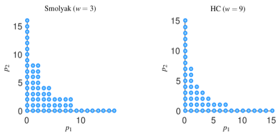
Figure 3. Index sets for Smolyak (SM) sparse grid for $N=2$ and $w=3$. The Hyperbolic Cross (HC) index set is also shown for $N=2$ and $w=9$, see [7] for details.

The Smolyak sparse grid combined with Clenshaw-Curtis (extrema of Chebyshev polynomials) abscissas leads to nested sequences of one dimensional interpolation formulas and a sparse grid with a highly reduced number of nodes compared to the corresponding tensor grid. For any choice of $m(i)>1$ the Clenshaw-Curtis abscissas are given by

$$\mathbcal{y}^{n}_{j}=-cos\left(\frac{\pi(j-1)}{m(i)-1}\right).$$

It is also straightforward to build related anisotropic sparse approximation formulas by making the function $g$ to act differently on the input random variables $y_{n}$ for $n=1,\dots,N$. Anisotropic sparse grids have been developed in [37, 31].

5. Error analysis

In this section error estimates of the mean and variance of the QoI are derived with respect to the sparse grid approximation and the truncation of the stochastic model to the first $N_{s}$ dimensions. The error contributions from the finite element and implicit solvers are neglected since there are many methods that can be used to solve the parabolic equation (e.g. [26]) and the analysis can be easily adapted. First, we establish some notation and assumptions:

1. Split the Jacobian matrix as follows

   (22) $$\partial F(\boldsymbol{\beta},\omega)=I+\sum_{l=1}^{N_{s}}\sqrt{\mu_{l}}\partial\mathbf{b}_{l}(\boldsymbol{\beta})Y_{l}(\omega)+\sum_{l=N_{s}+1}^{N}\sqrt{\mu_{l}}\partial\mathbf{b}_{l}(\boldsymbol{\beta})Y_{l}(\omega).$$

   and let $\Gamma_{s}:=[-1,1]^{N_{s}}$, ${\color[rgb]{0,0,0}\Gamma_{\kappa}}:=[-1,1]^{N-N_{s}}$, then the domain $\Gamma=\Gamma_{s}\times{\color[rgb]{0,0,0}\Gamma_{\kappa}}$.

2. In practice one is interested in computing the statistics of a Quantity of Interest (QoI) of the solution over the stochastic domain or a subdomain of it. Assume that $Q:L^{2}(U)\rightarrow\R$ is a bounded linear functional on $L^{2}(U)$ with norm $\|\cdot\|$.

3. Refer to $Q({\bf y}_{s})$ as $Q({\bf y})$ restricted to the stochastic domain $\Gamma_{s}$ and similarly for $G({\bf y}_{s})$. It is clear also that $Q({\bf y}_{s},{\color[rgb]{0,0,0}_{\kappa}})=Q({\bf y})$ and $G({\bf y}_{s},{\color[rgb]{0,0,0}_{\kappa}})=G({\bf y})$ for all ${\bf y}\in\Gamma_{s}\times{\color[rgb]{0,0,0}\Gamma_{\kappa}}$, ${\bf y}_{s}\in\Gamma_{s}$, and ${\color[rgb]{0,0,0}_{\kappa}}\in{\color[rgb]{0,0,0}\Gamma_{\kappa}}$.

4. Suppose that the $N_{{\bf g}}<N_{{\bf f}}$ valued random vector ${\bf g}=[f_{1},\dots,f_{N_{{\bf g}}}]$ matches with ${\bf f}$ from the first to $N_{{\bf f}}$ entry and takes values on $\Gamma_{{\bf g}}:=\tilde{\Gamma}_{1}\times\dots\times\tilde{\Gamma}_{N_{{\bf g}}}$. The truncated forcing function can now be written as

   $$(f\circ F)(\boldsymbol{\beta},{\bf g},{\bf y},t)=\sum_{n=1}^{N_{{\bf g}}}c_{n}(t,f_{n})(\xi_{n}\circ F)(\boldsymbol{\beta},{\bf y}).$$

It is not hard to show that the variance error ($|var[Q({\bf y}_{s},{\color[rgb]{0,0,0}_{\kappa}},{\bf f},t)]-var[\mathcal{S}^{m,g}_{w}[Q$ $({\bf y}_{s},{\color[rgb]{0,0,0}},t)]]|$) and mean error ($|{\mathbb{E}}\left[Q({\bf y}_{s},{\color[rgb]{0,0,0}_{\kappa}},{\bf f},t)\right]-{\mathbb{E}}\left[\mathcal{S}^{m,g}_{w}[Q({\bf y}_{s},{\color[rgb]{0,0,0}},t)\right]]|$) are less or equal to (see [7])

$$\begin{split}&C_{TR}\underbrace{\|Q({\bf y}_{s},{\color[rgb]{0,0,0}_{\kappa}},{\bf f},t)-Q({\bf y}_{s},{\bf f},t)\|_{L^{2}_{\rho}(\Gamma\times\Gamma_{{\bf f}})}}_{\mbox{Truncation (I)}}\\ &{\color[rgb]{0,0,0}+C_{FTR}\underbrace{\|Q({\bf y}_{s},{\bf f},t)-Q({\bf y}_{s},{\bf g},t)\|_{L^{2}_{\rho}(\Gamma\times\Gamma_{{\bf f}})}}_{\mbox{Forcing function Truncation (II)}}}\\ &+C_{SG}\underbrace{\|Q({\bf y}_{s},{\color[rgb]{0,0,0}},t)-\mathcal{S}^{m,g}_{w}[Q({\bf y}_{s},{\color[rgb]{0,0,0}},t)]\|_{L^{2}_{\rho}(\Gamma_{s}\times\Gamma_{{\color[rgb]{0,0,0}}})}}_{\mbox{{\color[rgb]{0,0,0}Sparse Grid (III)}}},\end{split}$$

where $C_{TR}$, $C_{FTR}$ and $C_{SG}$ are positive constants and $t\in(0,T)$. We now derive error estimates for the truncation (I) and sparse grid (II) errors.

5.1. Truncation error (I)

Given that $Q:L^{2}(U)\rightarrow\mathbb{R}$ is a bounded linear functional then

$$\begin{split}|Q({\bf y}_{s},{\color[rgb]{0,0,0}_{\kappa}},{\bf f},t)-Q({\bf y}_{s},{\color[rgb]{0,0,0}},t)|&\leq\|Q\|\|\hat{u}({\bf y}_{s},{\color[rgb]{0,0,0}_{\kappa}},{\bf f},t)-\hat{u}({\bf y}_{s},{\color[rgb]{0,0,0}},t)\|_{L^{2}(U)}.\end{split}$$

It follows that for $t\in(0,T)$

$$\begin{split}&\|Q({\bf y}_{s},{\color[rgb]{0,0,0}_{\kappa}},{\bf f},t)-Q({\bf y}_{s},{\bf f},t)\|_{L^{2}_{\rho}(\Gamma\times\Gamma_{{\bf f}})}\\ &\leq\|Q\|\|\hat{u}({\bf y}_{s},{\color[rgb]{0,0,0}_{\kappa}},{\bf f},t)-\hat{u}({\bf y}_{s},{\bf f},t)\|_{L^{2}_{\rho}(\Gamma\times\Gamma_{{\bf f}};L^{2}(U))}.\end{split}$$

The objective now is to control the error term $\|\hat{u}({\bf y},{\bf f},t)-\hat{u}({\bf y}_{s},{\bf f},t)\|_{L^{2}_{\rho}(\Gamma\times\Gamma_{{\bf f}};L^{2}(U))}$. But first we establish some notation. If $W$ is a Banach space defined on $U$ then let

$$C^{0}(\Gamma;W):=\{v:\Gamma\rightarrow W\,\,\mbox{is continuous on $\Gamma$ and }{\color[rgb]{0,0,0}\max_{{\bf y}\in\Gamma}\|v({\bf y})\|_{W}}<\infty\}.$$

and

$$L^{2}_{\rho}(\Gamma;W):=\{v:\Gamma\rightarrow W\,\,\mbox{is strongly measurable and}\,\,\int_{\Gamma}\|v\|^{2}_{W}\,\rho({\bf y})\,\mbox{d}{\bf y}<\infty\}.$$

With a slight abuse of notation let ${\color[rgb]{0,0,0}\hat{\varsigma}}({\bf y}_{s},{\bf f},t):=\hat{u}({\bf y}_{s},{\bf f},t)$ for all $t\in(0,T)$, ${\bf y}_{s}\in\Gamma_{s}$ and ${\bf f}\in\Gamma_{{\bf f}}$. From Theorem 2 it follows that

$${\color[rgb]{0,0,0}\hat{\varsigma}},\hat{u}\in C^{0}(\Gamma\times\Gamma_{{\bf f}};L^{2}(0,T;V))\subset L^{2}_{\rho}(\Gamma\times\Gamma_{{\bf f}};L^{2}(0,T;V)).$$

The following theorem provides error bounds on the truncation error. It is adapted from Theorem 10 in [7].

Theorem 3.

Suppose that ${\color[rgb]{0,0,0}\hat{\varsigma}}\in C^{0}(\Gamma_{s};L^{2}(0,T;V))$ satisfies

(23) $$\int_{U}|\partial F({\bf y}_{s})|v\partial_{t}{\color[rgb]{0,0,0}\hat{\varsigma}}\,\mbox{d}\boldsymbol{\beta}+{\color[rgb]{0,0,0}B({\bf y}_{s};{\color[rgb]{0,0,0}\hat{\varsigma}},v)}=\hat{l}({\bf y}_{s};{\bf f},v)\,\,\,\forall v\in V$$

for all ${\bf f}\in\Gamma_{{\bf f}}$, where ${\color[rgb]{0,0,0}\hat{\varsigma}}({\bf y}_{s},{\bf f},0)=u_{0}$. Let $e({\bf y},{\bf f},t):=\hat{u}({\bf y},{\bf f},t)-{\color[rgb]{0,0,0}\hat{\varsigma}}({\bf y}_{s},{\bf f},t)$,

$$B_{\T}:=\sup_{\boldsymbol{\beta}\in U}\sum_{l=N_{s}+1}^{N}\sqrt{\mu_{l}}\|\partial\mathbf{b}_{l}\|\,\,\mbox{and}\,\,C_{\T}:=\sum_{i=N_{s}+1}^{N}\sqrt{\mu_{l}}{\color[rgb]{0,0,0}\|\mathbf{b}_{l}\|_{[L^{\infty}(U)]^{d}}}$$

then for $0<t<T$, ${\bf f}\in\Gamma_{{\bf f}}$, it follows that

$$\begin{split}\|e({\bf y},{\bf f},t)\|^{2}_{L^{2}_{\rho}(\Gamma\times\Gamma_{{\bf f}};L^{2}(U))}&\leq\mathbb{C}_{1}B_{\T}+\mathbb{C}_{2}C_{\T}(1+C_{\T}),\end{split}$$

where

$$\begin{split}&\mathbb{C}_{1}(T,C_{{\mathcal{T}}},D_{{\mathcal{T}}},C_{T}(U),C_{P}(U),\F_{max},\F_{min},\tilde{\delta},d,a_{max},\|g_{N}\|_{W^{1,\infty}(\mathcal{G}_{N})},\\ &\sup_{t\in(0,T)}{\mathbb{E}}\left[\|\hat{u}({\bf y},{\bf f},t)\|^{2}_{V}\right],\sup_{\small{{\begin{array}[]{c}t\in(0,T)\\ {\bf f}\in\Gamma_{{\bf f}},{\bf y}\in\Gamma\end{array}}}}\|(f\circ F)({\bf y},{\bf f},t)\|_{L^{2}(U)},\\ &\sup_{t\in(0,T)}{\mathbb{E}}\left[\|\partial_{t}{\color[rgb]{0,0,0}\hat{\varsigma}}({\bf y}_{s},{\bf f},t)\|^{2}_{L^{2}(U)}\right]^{\frac{1}{2}},{\mathbb{E}}\left[\|\hat{u}({\bf y},{\bf f},t)\|^{2}_{V}\right]^{\frac{1}{2}},\sup_{{\bf x}^{\prime}\in B^{0}_{r},\tau\in{\mathcal{T}}}\|{\bf J}_{\tau}({\bf x}^{\prime})\|)\\ &\mathbb{C}_{2}(T,S_{{\mathcal{T}}},C_{{\mathcal{T}}},C_{T}(U),C_{P}(U),\F_{max},\F_{min},d,\sup_{{\bf f}\in\Gamma_{{\bf f}}}\|f\|_{W^{1,\infty}({\mathcal{G}}\times(0,T))},\|a\|_{W^{1,\infty}({\mathcal{G}})},\\ &\|g_{N}\|_{W^{1,\infty}(\partial{\mathcal{G}}_{N})},\|\chi_{U}\|_{L^{2}(U)},\\ &\sup_{t\in(0,T)}{\color[rgb]{0,0,0}{\mathbb{E}}\left[\|\hat{u}({\bf y},{\bf f},t)\|^{2}_{V}\right]},\|u_{0}\|_{W^{1,\infty}({\mathcal{G}})})\end{split}$$

are constants, $C_{T}(U)$ is the Trace Theorem constant, $C_{P}(U)$ is the Poincaré constants, $C_{{\mathcal{T}}}:=(\inf_{{\bf x}^{\prime}\in B^{0}_{r},\tau\in{\mathcal{T}}}$ $\sigma^{d-1}_{min}({\bf J}_{\tau}^{T}{\bf J}_{\tau}))^{-1}$, $S_{{\mathcal{T}}}:=\sup_{{\bf x}^{\prime}\in B^{0}_{r},\tau\in{\mathcal{T}},{\bf y}\in\Gamma}|s((\boldsymbol{\beta}\circ\xi_{\tau})({\bf x}^{\prime}),{\bf y})^{\frac{1}{2}}|$ , and $D_{{\mathcal{T}}}:=(\inf_{{\bf x}^{\prime}\in B^{0}_{r},\tau\in{\mathcal{T}},{\bf y}\in\Gamma}|s((\boldsymbol{\beta}\circ\xi_{\tau})({\bf x}^{\prime}),{\bf y})^{\frac{1}{2}}|)^{-1}$.

$$\chi_{U}(\boldsymbol{\beta})=\left\{\begin{array}[]{l l c}1&&\boldsymbol{\beta}\in U\\ 0&&o.w.\end{array}\right..$$

Proof.

Consider the solution to equation (23)

$${\color[rgb]{0,0,0}\hat{\varsigma}}\in C^{0}(\Gamma_{s}\times\Gamma_{{\bf f}};L^{2}(0,T;V))\subset L^{2}_{\rho}(\Gamma\times\Gamma_{{\bf f}};L^{2}(0,T;V))$$

where the matrix of coefficients $G({\bf y}_{s})$ depends only on the variables $Y_{1},\dots,Y_{N_{s}}$. By adapting the proof from Strang’s Lemma we have that

$$\begin{split}\|{\color[rgb]{0,0,0}\hat{\varsigma}}({\bf y}_{s})-\hat{u}({\bf y})\|^{2}_{V}&\leq{\mathbb{K}}\Big{(}\left|\hat{l}({\bf y}_{s};{\color[rgb]{0,0,0}\hat{\varsigma}}({\bf y}_{s})-\hat{u}({\bf y}))-\hat{l}({\bf y};{\color[rgb]{0,0,0}\hat{\varsigma}}({\bf y}_{s})-\hat{u}({\bf y}))\right|\\ &+\int_{U}({\color[rgb]{0,0,0}\hat{\varsigma}}({\bf y}_{s})-\hat{u}({\bf y}))(|\partial F({\bf y})|-|\partial F({\bf y}_{s})|)\partial_{t}{\color[rgb]{0,0,0}\hat{\varsigma}}({\bf y}_{s}))\\ &+\int_{U}({\color[rgb]{0,0,0}\hat{\varsigma}}({\bf y}_{s})-\hat{u}({\bf y}))(|\partial F({\bf y})|(\partial_{t}\hat{u}({\bf y})-\partial_{t}{\color[rgb]{0,0,0}\hat{\varsigma}}({\bf y}_{s})))\\ &+\left|B({\bf y};\hat{u}({\bf y}),{\color[rgb]{0,0,0}\hat{\varsigma}}({\bf y}_{s})-\hat{u}({\bf y}))-B({\bf y}_{s};\hat{u}({\bf y}),{\color[rgb]{0,0,0}\hat{\varsigma}}({\bf y}_{s})-\hat{u}({\bf y})))\right|\Big{)},\end{split}$$

where ${\mathbb{K}}:=a_{min}^{-1}\F_{min}^{-d}\F_{max}^{2}(1+C_{P}(U)^{2})$. Recall that $e({\bf y}):=\hat{u}({\bf y})-{\color[rgb]{0,0,0}\hat{\varsigma}}({\bf y}_{s})$ and note that

$$\begin{split}\int_{U}e({\bf y})|\partial F({\bf y})|^{\frac{1}{2}}\partial_{t}{\color[rgb]{0,0,0}\left(|\partial F({\bf y})|^{\frac{1}{2}}e({\bf y})\right)}&=\frac{1}{2}\partial_{t}\|e({\bf y})|\partial F({\bf y})|^{\frac{1}{2}}\|^{2}_{L^{2}(U)}\\ &\geq\frac{\F_{min}^{d}}{2}\partial_{t}\|e({\bf y})\|^{2}_{L^{2}(U)}\end{split}$$

thus

$$\begin{split}\frac{\F^{d}_{min}}{2}\partial_{t}\|e({\bf y})\|^{2}_{L^{2}(U)}&\leq\Big{(}\left|\hat{l}({\bf y};e({\bf y}))-\hat{l}({\bf y}_{s};e({\bf y}))\right|\\ &+\left|B({\bf y};\hat{u}({\bf y}),e({\bf y}))-B({\bf y}_{s};\hat{u}({\bf y}),e({\bf y})))\right|\\ &+\int_{U}\left|e({\bf y})(|\partial F({\bf y})|-|\partial F({\bf y}_{s})|)\partial_{t}{\color[rgb]{0,0,0}\hat{\varsigma}}({\bf y}_{s})\right|\Big{)}.\end{split}$$

and for all $t\in(0,T)$, ${\bf f}\in\Gamma_{{\bf f}}$ and ${\bf y}\in\Gamma$

$$\begin{split}\partial_{t}\|e({\bf y},{\bf f},t)\|^{2}_{L^{2}(U)}&\leq\frac{2}{\F^{d}_{min}}({\mathbb{B}}_{1}+{\mathbb{B}}_{2}+{\mathbb{B}}_{3})\end{split}$$

for some non-negative constants ${\mathbb{B}}_{1},{\mathbb{B}}_{2},{\mathbb{B}}_{3}<\infty$. For now assume that ${\mathbb{B}}_{1}$, ${\mathbb{B}}_{2}$ and ${\mathbb{B}}_{3}$ are known. From Gronwall’s inequality we have that for $t\in(0,T)$, ${\bf y}\in\Gamma$, and ${\bf f}\in{\color[rgb]{0,0,0}\Gamma_{{\bf f}}}$

(24) $$\begin{split}\|e({\bf y},{\bf f},t)\|^{2}_{L^{2}(U)}&\leq\|e({\bf y},{\bf f},0)\|^{2}_{L^{2}(U)}+\frac{2({\mathbb{B}}_{1}+{\mathbb{B}}_{2}+{\mathbb{B}}_{3})T}{\F_{min}^{d}}\end{split}$$

The first term in equation (24) is bounded as

(25) $$\begin{split}\|e({\bf y},{\bf f},0)\|_{L^{2}(U)}&=\|(u_{0}\circ F)({\bf y}_{s})-(u_{0}\circ F)({\bf y})\|_{L^{2}(U)}\\ &\leq\|u_{0}\|_{W^{1,\infty}({\mathcal{G}})}\|\chi_{U}\|_{L^{2}(U)}\sup_{{\bf y}\in\Gamma,\boldsymbol{\beta}\in U}|F({\bf y}_{s})-F({\bf y})|,\end{split}$$

for all ${\bf f}\in\Gamma_{{\bf f}}$ and ${\bf y}\in\Gamma$. For the second term we have that

$$\begin{split}&{\mathbb{B}}_{1}:={\color[rgb]{0,0,0}\sup_{t\in(0,T)}}|B({\bf y};\hat{u}({\bf y},{\bf f},t),e({\bf y},{\bf f},t))-B({\bf y}_{s};\hat{u}({\bf y},{\bf f},t),e({\bf y},{\bf f},t))|\\ &\leq{\color[rgb]{0,0,0}\sup_{t\in(0,T)}}\|\hat{u}({\bf y},{\bf f},t)\|_{V}(\|\hat{u}({\bf y},{\bf f},t)\|_{V}+\|{\color[rgb]{0,0,0}\hat{\varsigma}}({\bf y}_{s},{\bf f},t)\|_{V})\sup_{\boldsymbol{\beta}\in U,{\bf y}\in\Gamma}\|G({\bf y})-G({\bf y}_{s})\|.\end{split}$$

Following the same argument for Theorem 10 in [7] we have that

(26) $$\sup_{\boldsymbol{\beta}\in U,{\bf y}\in\Gamma}\|G({\bf y})-G({\bf y}_{s})\|\leq a_{max}B_{\T}H(\F_{max},\F_{min},\tilde{\delta},d)$$

for some constant $H(\F_{max},\F_{min},\tilde{\delta},d)$. Thus we have

(27) $$\begin{split}{\mathbb{E}}\left[{\mathbb{B}}_{1}\right]&\leq a_{max}B_{\T}H(\F_{max},\F_{min},\tilde{\delta},d){\color[rgb]{0,0,0}\sup_{t\in(0,T)}2{\mathbb{E}}\left[\|\hat{u}({\bf y},{\bf f},t)\|^{2}\right].}\end{split}$$

The last term is true since $\hat{u}$ and ${\color[rgb]{0,0,0}\hat{\varsigma}}$ are equal when ${\bf y}=[{\bf y}_{s},0]^{T}$

$${\mathbb{E}}\left[\|{\color[rgb]{0,0,0}\hat{\varsigma}}({\bf y}_{s},{\bf f},t)\|^{p}_{V}\right]\leq{\mathbb{E}}\left[\|\hat{u}({\bf y},{\bf f},t)\|^{p}_{V}\right],$$

$p=1,2,\dots$ where the expectation ${\mathbb{E}}\left[\cdot\right]$ is defined over the domain $\Gamma$ and $\Gamma_{{\bf f}}$. The next constant

$${\mathbb{B}}_{2}:=|\hat{l}({\bf y};e({\bf y},{\bf f},t))-\hat{l}({\bf y}_{s};e({\bf y},{\bf f},t))|$$

is bounded by

(28) $$\begin{split}&\Big{|}\int_{U}((f\circ F)({\bf y},{\bf f},t)|\partial F({\bf y})|-(f\circ F)({\bf y}_{s},{\bf f},t)|\partial F({\bf y}_{s})|)e({\bf y},{\bf f},t)\Big{|}\\ &+{\color[rgb]{0,0,0}\Big{|}\sum_{\tau\in{\mathcal{T}}}\int_{B^{0}_{r}}((g_{N}\circ F)(\boldsymbol{\beta},{\bf y})s(\boldsymbol{\beta},{\bf y})^{\frac{1}{2}}-(g_{N}\circ F)(\boldsymbol{\beta},{\bf y}_{s})s(\boldsymbol{\beta},{\bf y}_{s})^{\frac{1}{2}})e({\bf y},{\bf f},t)\,\mbox{d}{\bf x}^{\prime}\Big{|}}\\ &\leq{\color[rgb]{0,0,0}\sum_{\tau\in{\mathcal{T}}}\int_{B^{0}_{r}}|((g_{N}\circ F)(\boldsymbol{\beta},{\bf y})-(g_{N}\circ F)(\boldsymbol{\beta},{\bf y}_{s}))s(\boldsymbol{\beta},{\bf y}))^{\frac{1}{2}}e({\bf y},{\bf f},t)|}\\ &{\color[rgb]{0,0,0}+|(g_{N}\circ F)(\boldsymbol{\beta},{\bf y}_{s})(s(\boldsymbol{\beta},{\bf y})^{\frac{1}{2}}-s(\boldsymbol{\beta},{\bf y}_{s})^{\frac{1}{2}})e({\bf y},{\bf f},t)|\,\mbox{d}{\bf x}^{\prime}}\\ &+\int_{U}|((f\circ F)({\bf y},{\bf f},t)-(f\circ F)({\bf y}_{s},{\bf f},t))|\partial F({\bf y})|e({\bf y},{\bf f},t)|\\ &+|(f\circ F)({\bf y}_{s},{\bf f},t)(|\partial F({\bf y})|-|\partial F({\bf y}_{s})|)e({\bf y},{\bf f},t)|\\ \end{split}$$

for all $t\in(0,T)$, ${\bf f}\in\Gamma_{{\bf f}}$ and ${\bf y}\in\Gamma$. The following inequalities are used to bound equation (28):

(29a) $$\sum_{\tau\in{\mathcal{T}}}\int_{B^{0}_{r}}|((g_{N}\circ F)(\boldsymbol{\beta},{\bf y})-(g_{N}\circ F)(\boldsymbol{\beta},{\bf y}_{s}))s(\boldsymbol{\beta},{\bf y})^{\frac{1}{2}})e({\bf y},{\bf f},t)|$$

$$\leq C_{{\mathcal{T}}}S_{{\mathcal{T}}}\|e({\bf y},{\bf f},t)\|_{L^{2}(\partial U)}\|g_{N}\|_{W^{1,\infty}(\partial{\mathcal{G}}_{N})}\sup_{{\bf y}\in\Gamma,\boldsymbol{\beta}\in U}|F({\bf y})-F({\bf y}_{s})|$$

$$(\mbox{Using the Trace Theorem \cite[cite]{[\@@bibref{}{Evans1998}{}{}]}}:\|e({\bf y},{\bf f},t)\|_{L^{2}(\partial U)}\leq C_{T}(U)\|e({\bf y},{\bf f},t)\|_{H^{1}(U)}),$$

(29b) $$\sum_{\tau\in{\mathcal{T}}}\int_{B^{0}_{r}}|(g_{N}\circ F)(\boldsymbol{\beta},{\bf y}_{s})(s(\boldsymbol{\beta},{\bf y})^{\frac{1}{2}}-s(\boldsymbol{\beta},{\bf y}_{s})^{\frac{1}{2}})e({\bf y},{\bf f},t)|$$

$$\leq\frac{D_{{\mathcal{T}}}C_{{\mathcal{T}}}C_{T}(U)}{2}\|e({\bf y},{\bf f},t)\|_{H^{1}(U)}\|g_{N}\|_{W^{1,\infty}(\partial{\mathcal{G}}_{N})}\sup_{\tau\in{\mathcal{T}}}|det({\bf J}_{\tau}^{T}\partial F(\boldsymbol{\beta}\circ\xi_{\tau},{\bf y})^{T}$$

$$\partial F(\boldsymbol{\beta}\circ\xi_{\tau},{\bf y}){\bf J}_{\tau})-det({\bf J}_{\tau}^{T}\partial F(\boldsymbol{\beta}\circ\xi_{\tau},{\bf y}_{s})^{T}\partial F(\boldsymbol{\beta}\circ\xi_{\tau},{\bf y}_{s}){\bf J}_{\tau})|$$

(29c) $$\int_{U}|((f\circ F)({\bf y},{\bf f},t)-(f\circ F)({\bf y}_{s},{\bf f},t))|\partial F({\bf y})|e({\bf y},{\bf f},t)$$

$$\leq\F_{max}^{d}\|\chi_{U}\|_{L^{2}(U)}\sup_{{\bf f}\in\Gamma_{{\bf f}}}\|f\|_{W^{1,\infty}({\mathcal{G}}\times(0,T))}$$

$$\|e({\bf y},{\bf f},t)\|_{V}\sup_{{\bf y}\in\Gamma,\boldsymbol{\beta}\in U}|F({\bf y})-F({\bf y}_{s})|,$$

(29d) $$\int_{U}|(f\circ F)({\bf y}_{s},{\bf f},t)(|\partial F({\bf y})|-|\partial F({\bf y}_{s})|)e({\bf y},{\bf f},t)|$$

(29g) $$\leq\|e({\bf y},{\bf f},t)\|_{V}\sup_{\small{{\begin{array}[]{c}t\in(0,T)\\ {\bf f}\in\Gamma_{{\bf f}},{\bf y}\in\Gamma\end{array}}}}\|(f\circ F)({\bf y},{\bf f},t)\|_{L^{2}(U)}$$

$$\sup_{{\bf y}\in\Gamma,\boldsymbol{\beta}\in U}||\partial F({\bf y})|-|\partial F({\bf y}_{s})||,$$

Following the same argument for Theorem 10 in [7] we have that

(30) $$\sup_{{\bf y}\in\Gamma}||\partial F({\bf y})|-|\partial F({\bf y}_{s})||\leq\F_{max}^{d-1}\F^{-2}_{min}dB_{\T},$$

(31) $$\sup_{\boldsymbol{\beta}\in U,{\bf y}\in\Gamma}|F({\bf y})-F({\bf y}_{s})|\leq C_{\T}.$$

From Theorem 2.12 in [22] ($A,E\in\C^{d\times d}$ then $|det(A+E)-det(A)|\leq d\|E\|$ $\max\{\|A\|,$ $\|A+E\|\}^{d-1})$ we obtain $\forall x\in U$ and $\forall{\bf y}\in\Gamma$

(32) $$\begin{split}&|det({\bf J}_{\tau}^{T}\partial F(\boldsymbol{\beta}\circ\xi_{\tau},{\bf y})^{T}\partial F(\boldsymbol{\beta}\circ\xi_{\tau},{\bf y}){\bf J}_{\tau})-det({\bf J}_{\tau}^{T}\partial F(\boldsymbol{\beta}\circ\xi_{\tau},{\bf y}_{s})^{T}\\ &\partial F(\boldsymbol{\beta}\circ\xi_{\tau},{\bf y}_{s}){\bf J}_{\tau})|\leq\sup_{{\bf x}^{\prime}\in B^{0}_{r},\tau\in{\mathcal{T}}}\|{\bf J}_{\tau}({\bf x}^{\prime})\|^{2d}d\F_{max}^{2d-1}B_{\T}.\end{split}$$

Furthermore using Jensen’s inequality

(33) $${\mathbb{E}}\left[\|e({\bf y},{\bf f},t)\|_{V}\right]\leq C{\mathbb{E}}\left[\|\hat{u}({\bf y},{\bf f},t)\|_{V}\right]\leq C{\mathbb{E}}\left[\|\hat{u}({\bf y},{\bf f},t)\|^{2}_{V}\right]$$

for some constant $C>0$. Combining inequalities (29) (a) - (g) and equations (28), (30) - (33)

$$\begin{split}&{\mathbb{E}}\left[{\mathbb{B}}_{2}\right]\leq\Xi(C_{T}(U),S_{{\mathcal{T}}},C_{{\mathcal{T}}},\F_{max},\F_{min},d,\sup_{{\bf f}\in\Gamma_{{\bf f}}}\|f\|_{W^{1,\infty}({\mathcal{G}}\times(0,T))},\|a\|_{W^{1,\infty}({\mathcal{G}})},\\ &\|g_{N}\|_{W^{1,\infty}(\partial{\mathcal{G}}_{N})},\|\hat{{\color[rgb]{0,0,0}\varkappa}}\|_{W^{1,\infty}(\mathcal{G})},\|\chi_{U}\|_{L^{2}(U)},\\ &\sup_{t\in(0,T)}{\mathbb{E}}\left[\|\hat{u}({\bf y},{\bf f},t)\|^{2}_{V}\right])C_{\T}+\Upsilon(C_{T}(U),C_{{\mathcal{T}}},D_{{\mathcal{T}}},\F_{max},\F_{min},\tilde{\delta},d,a_{max},\\ &\|\hat{g}_{N}\|_{W^{1,\infty}(\partial\mathcal{G}_{N})},\sup_{{\bf x}^{\prime}\in B^{0}_{r},\tau\in{\mathcal{T}}}\|{\bf J}_{\tau}({\bf x}^{\prime})\|,\\ &\sup_{t\in(0,T)}{\mathbb{E}}\left[\|\hat{u}({\bf y},{\bf f},t)\|^{2}_{V}\right],\sup_{\small{{\begin{array}[]{c}t\in(0,T)\\ {\bf f}\in\Gamma_{{\bf f}},{\bf y}\in\Gamma\end{array}}}}\|(f\circ F)({\bf y},{\bf f},t)\|_{L^{2}(U)})B_{\T},\end{split}$$

for some non-negative constants $\Xi$ and $\Upsilon$. The last constant

$$\begin{split}{\mathbb{B}}_{3}&\leq\int_{U}\left|e({\bf y},{\bf f},t)(|\partial F({\bf y})|-|\partial F({\bf y}_{s})|)\partial_{t}{\color[rgb]{0,0,0}\hat{\varsigma}}({\bf y}_{s},{\bf f})\right|\\ &\leq 2\F^{d-1}_{\max}\F^{-2}_{min}dB_{\T}\sup_{t\in(0,T)}\|\hat{u}({\bf y},{\bf f},t)\|_{V}\|\partial_{t}{\color[rgb]{0,0,0}\hat{\varsigma}}({\bf y}_{s},{\bf f},t)\|_{L^{2}(U)}.\end{split}$$

By using the Schwartz inequality ${\mathbb{E}}\left[{\mathbb{B}}_{3}\right]$ is less or equal to

$$\F^{d-1}_{\max}\F^{-2}_{min}dB_{\T}\sup_{t\in(0,T)}\Big{(}{\mathbb{E}}\left[\|\hat{u}({\bf y},{\bf f},t)\|^{2}_{V}\right]\Big{)}^{1/2}\Big{(}{\mathbb{E}}\left[\|\partial_{t}{\color[rgb]{0,0,0}\hat{\varsigma}}({\color[rgb]{0,0,0}_{s}},{\bf f},t)\|^{2}_{L^{2}(U)}\right]\Big{)}^{1/2}.$$

Combining the bounds for ${\mathbb{E}}\left[{\mathbb{B}}_{1}\right]$ , ${\mathbb{E}}\left[{\mathbb{B}}_{2}\right]$, ${\mathbb{E}}\left[{\mathbb{B}}_{3}\right]$, equations (25) and (24) we obtain the result. ∎

5.2. Forcing function truncation error (II)

Since $Q$ is a bounded linear functional the error due to (II) is controlled by $\|\hat{u}({\bf y}_{s},{\bf f},t)-\hat{u}({\bf y}_{s},{\bf g},t)\|_{L^{2}_{\rho}(\Gamma\times\Gamma_{{\bf f}};L^{2}(U))}$. Suppose that $\hat{u}({\bf y}_{s},{\bf f},t)\in L^{2}(0,T;V)$ satisfies the following equation

(34) $$\int_{U}|\partial F({\bf y}_{s})|v\partial_{t}\hat{u}\,\mbox{d}\boldsymbol{\beta}+B({\bf y}_{s};\hat{u},v)=\hat{l}({\bf y}_{s};{\bf f},v)\,\,\,\forall v\in V$$

for all ${\bf f}\in\Gamma_{{\bf f}}$ and ${\bf y}_{s}\in\Gamma_{s}$, where $\hat{u}({\bf y}_{s},{\bf f},0)=u_{0}$. Furthermore, let $\hat{u}({\bf y}_{s},{\bf g},t)\in L^{2}(0,T;V))$ satisfies

(35) $$\int_{U}|\partial F({\bf y}_{s})|v\partial_{t}\hat{u}\,\mbox{d}\boldsymbol{\beta}+B({\bf y}_{s};\hat{u},v)=\hat{l}({\bf y}_{s};{\bf g},v)\,\,\,\forall v\in V$$

for all ${\bf g}\in\Gamma_{{\bf g}}$ and ${\bf y}_{s}\in\Gamma_{s}$, where $\hat{u}({\bf y}_{s},{\bf g},0)=u_{0}$.

Theorem 4.

Let $\hat{e}({\bf y}_{s},{\bf f},t):=\hat{u}({\bf y}_{s},{\bf f},t)-\hat{u}({\bf y}_{s},{\bf g},t)$, $t\in(0,T)$,

$$0<\epsilon<a_{min}^{-1}\F_{min}^{-d}\F^{2}_{max}C_{P}(U)^{2}/4$$

and

$${\mathcal{J}}(d,a_{min},\F_{min},\F_{max},C_{P}(U),\epsilon):=\frac{2}{\F_{min}^{d}}\left[\frac{1}{4\varepsilon}-a_{min}\F^{d}_{min}\F^{-2}_{max}C_{P}(U)^{-2}\right]$$

then

$$\begin{split}&\|\hat{e}({\bf y}_{s},{\bf f},t)\|_{L^{2}_{\rho}(\Gamma\times\Gamma_{{\bf f}};U)}\leq T^{1/2}e^{{\mathcal{J}}(d,a_{min},\F_{min},\F_{max},C_{P}(U),\epsilon)T/2}\\ &\epsilon^{1/2}\left(\sum_{n=N_{{\bf g}}+1}^{N_{{\bf f}}}{\mathbb{E}}\left[c^{2}_{n}(t,f_{n})\right]\right)^{1/2}\left(\sum_{n=N_{{\bf g}}+1}^{N_{{\bf f}}}\|(\xi_{n}\circ F)(\boldsymbol{\beta},{\bf y}_{s})\|^{2}_{L^{2}_{\rho}(\Gamma_{s};U)}\right)^{1/2}.\end{split}$$

Proof.

Subtract (35) from (34)

(36) $$\int_{U}|\partial F({\bf y}_{s})|v\partial_{t}\hat{e}\,\mbox{d}\boldsymbol{\beta}+B({\bf y}_{s};\hat{e},v)=\int_{U}((f\circ F)(\cdot,{\bf y}_{s},{\bf f})-(f\circ F)(\cdot,{\bf y}_{s},{\bf g}))v$$

$\forall v\in V$. Recall that

$$\begin{split}\int_{U}\hat{e}|\partial F({\bf y}_{s})|^{\frac{1}{2}}\partial_{t}\left(|\partial F({\bf y}_{s})|^{\frac{1}{2}}\hat{e}\right)&=\frac{1}{2}\partial_{t}\|\hat{e}|\partial F({\bf y}_{s})|^{\frac{1}{2}}\|^{2}_{L^{2}(U)}.\end{split}$$

Let $v=\hat{e}$ and substitute in (36), then

$$\begin{split}&\frac{1}{2}\partial_{t}\|\hat{e}|\partial F({\bf y}_{s})|^{\frac{1}{2}}\|^{2}_{L^{2}(U)}+B({\bf y}_{s};\hat{e},\hat{e})\\ &=\int_{U}((f\circ F)(\cdot,{\bf y}_{s},{\bf f})-(f\circ F)(\cdot,{\bf y}_{s},{\bf g}))\hat{e}.\end{split}$$

Applying the Poincaré and Cauchy’s inequalities we obtain

$$\begin{split}&\frac{\F^{d}_{min}}{2}\partial_{t}\|\hat{e}\|^{2}_{L^{2}(U)}+a_{min}\F^{d}_{min}\F^{-2}_{max}C_{P}(U)^{-2}\|\hat{e}\|^{2}\\ &\leq\frac{1}{4\epsilon}\|\hat{e}\|^{2}_{L^{2}(U)}+\epsilon\|(f\circ F)(\cdot,{\bf y}_{s},{\bf f})-(f\circ F)(\cdot,{\bf y}_{s},{\bf g}))\|^{2}_{L^{2}(U)}.\end{split}$$

From Gronwall’s inequality it follows that

$$\begin{split}{\mathbb{E}}\left[\|\hat{e}\|^{2}_{L^{2}(U)}\right]&\leq Te^{{\mathcal{J}}(d,a_{min},\F_{min},\F_{max},C_{P}(U),\epsilon)T}\\ &\epsilon{\mathbb{E}}\left[\|(f\circ F)(\cdot,{\bf y}_{s},{\bf f})-(f\circ F)(\cdot,{\bf y}_{s},{\bf g}))\|^{2}_{L^{2}(U)}\right].\end{split}$$

We have that

$$\begin{split}&\|(f\circ F)(\cdot,{\bf y}_{s},{\bf f})-(f\circ F)(\cdot,{\bf y}_{s},{\bf g}))\|_{L^{2}(U)}\\ &\leq\|\sum_{n=N_{{\bf g}}+1}^{N_{{\bf f}}}c_{n}(t,{\bf f})(\xi_{n}\circ F)(\boldsymbol{\beta},{\bf y}_{s})\|_{L^{2}(U)}\\ &\leq\sum_{n=N_{{\bf g}}+1}^{N_{{\bf f}}}|c_{n}(t,f_{n})|\|(\xi_{n}\circ F)(\boldsymbol{\beta},{\bf y}_{s})\|_{L^{2}(U)}\\ &\leq\Big{(}\sum_{n=N_{{\bf g}}+1}^{N_{{\bf f}}}c^{2}_{n}(t,f_{n})\Big{)}^{1/2}\Big{(}\sum_{n=N_{{\bf g}}+1}^{N_{{\bf f}}}\|(\xi_{n}\circ F)(\boldsymbol{\beta},{\bf y}_{s})\|^{2}_{L^{2}(U)}\Big{)}^{1/2},\end{split}$$

thus

$$\begin{split}&{\mathbb{E}}\left[\|(f\circ F)(\cdot,{\bf y}_{s},{\bf f})-(f\circ F)(\cdot,{\bf y}_{s},{\bf g}))\|^{2}_{L^{2}(U)}\right]\\ &\leq\sum_{n=N_{{\bf g}}+1}^{N_{{\bf f}}}{\mathbb{E}}\left[c^{2}_{n}(t,f_{n})\right]\sum_{n=N_{{\bf g}}+1}^{N_{{\bf f}}}\|(\xi_{n}\circ F)(\boldsymbol{\beta},{\bf y}_{s})\|^{2}_{L^{2}_{\rho}(\Gamma_{s};U)}.\end{split}$$

∎

5.3. Sparse grid error (III)

In this section convergence rates for the isotropic Smolyak sparse grid with Clenshaw Curtis abscissas are derived. The convergence rates can be extended to a larger class of abscissas and anisotropic sparse grids following the same approach.

Given the bounded linear functional $Q:L^{2}(U)\rightarrow\R$ it follows that

$$\begin{split}|Q({\bf y}_{s},{\color[rgb]{0,0,0}},t)-\mathcal{S}^{m,g}_{w}[Q({\bf y}_{s},{\color[rgb]{0,0,0}},t)]|&\leq\|Q\|\|\hat{u}({\bf y}_{s},{\color[rgb]{0,0,0}},t)-\mathcal{S}^{m,g}_{w}[\hat{u}({\bf y}_{s},{\color[rgb]{0,0,0}},t)]\|_{L^{2}(U)}\end{split}$$

for all $t\in(0,T)$, ${\bf y}_{s}\in\Gamma_{s}$ and ${\color[rgb]{0,0,0}}\in\Gamma_{{\color[rgb]{0,0,0}}}$. The sparse grid operator $\mathcal{S}^{m,g}_{w}$ is with respect to the domain $\Gamma_{s}\times\Gamma_{{\color[rgb]{0,0,0}}}$. The next step it to bound the term

$$\|\hat{u}({\bf y}_{s},{\color[rgb]{0,0,0}},t)-\mathcal{S}^{m,g}_{w}[\hat{u}({\bf y}_{s},{\color[rgb]{0,0,0}},t)]\|_{L^{2}(\Gamma_{s}\times\Gamma_{{\color[rgb]{0,0,0}}};U)}.$$

for $t\in(0,T)$. The error term $\|\epsilon\|_{L^{2}(\Gamma_{s}\times\Gamma_{{\color[rgb]{0,0,0}}};U)}$, where

$$\epsilon:=\hat{u}({\bf y}_{s},{\color[rgb]{0,0,0}},T)-\mathcal{S}^{m,g}_{w}[\hat{u}({\bf y}_{s},{\color[rgb]{0,0,0}},T)],$$

is controlled by the number of collocation knots $\eta$ (or work), the choice of the approximation formulas $(m(i),g({\bf i}))$, and the region of analyticity of $\Theta_{\beta}\times{\color[rgb]{0,0,0}\mathscr{F}}\subset\mathbb{C}^{N_{s}+N_{{\color[rgb]{0,0,0}}}}$. From Theorem 2 the solution $\hat{u}({\bf y}_{s},{\color[rgb]{0,0,0}},t)$ admits an analytic extension in $\Theta_{\beta}\times{\color[rgb]{0,0,0}\mathscr{F}}\subset\C^{N_{s}+N_{{\color[rgb]{0,0,0}}}}$ for all $t\in(0,T)$.

In [31, 32] the authors derive error estimates for isotropic and anisotropic Smolyak sparse grids with Clenshaw-Curtis and Gaussian abscissas where $\|\epsilon\|_{{L^{2}_{\hat{\rho}}(\Gamma_{s};V})}$ exhibit algebraic or sub-exponential convergence with respect to the number of collocation knots $\eta$. For these estimates to be valid the solution $\hat{u}({\bf y}_{s},{\color[rgb]{0,0,0}},T)$ has to admit and extension on a polyellipse in $\C^{N_{s}+N_{{\color[rgb]{0,0,0}}}}$ i.e. ${\mathcal{E}}_{\sigma_{1},\dots,\sigma_{N_{s}+N_{{\color[rgb]{0,0,0}}}}}:=\Pi_{i=1}^{N_{s}+N_{{\color[rgb]{0,0,0}}}}$ ${\mathcal{E}}_{n,\sigma_{n}}$, where

$$\begin{split}{\mathcal{E}}_{n,\sigma_{n}}&=\left\{z\in\C;\,\mathop{\text{\rm Re}}(z)=\frac{e^{\sigma_{n}}+e^{-\sigma_{n}}}{2}cos(\theta),\right.\\ &\left.\mathop{\text{\rm Im}}(z)=\frac{e^{\sigma_{n}}-e^{-\sigma_{n}}}{2}sin(\theta),\theta\in[0,2\pi)\right\},\,\,\,\end{split}$$

and $\sigma_{n}>0$. For an isotropic sparse grid the overall asymptotic subexponential decay rate $\hat{\sigma}$ will be dominated by the smallest $\sigma_{n}$ i.e.

$$\hat{\sigma}\equiv\min_{n=1,\dots,N_{s}+N_{{\color[rgb]{0,0,0}}}}\sigma_{n}.$$

Then the goal is to choose the largest $\hat{\sigma}$ such that ${\mathcal{E}}_{\sigma_{1},\dots,\sigma_{N_{s}+N_{{\color[rgb]{0,0,0}}}}}\subset\Theta_{\beta}\times{\color[rgb]{0,0,0}\mathscr{F}}$. First, form the set $\Sigma\subset\C^{N_{s}}$ such that $\Sigma\subset\Theta_{\beta}$, where $\Sigma:=\Sigma_{1}\times\dots\times\Sigma_{N_{s}}$ and

$$\Sigma_{n}:=\left\{{\bf z}\in\mathbb{C};\,{\bf z}={\bf y}+{\bf v},\,{\bf y}\in[-1,1],\,|v_{n}|\leq\tau_{n}:=\frac{\beta}{1-\tilde{\delta}}\right\},$$

for $n=1,\dots,N_{s}$. Let

$$\hat{\sigma}_{\beta}:=\log{\left(\sqrt{\left(\frac{\beta}{1-\tilde{\delta}}\right)^{2}+1}+\frac{\beta}{1-\tilde{\delta}}\right)}>0,$$

then the polyellipse ${\mathcal{E}}_{\sigma_{1},\dots,\sigma_{N_{{\color[rgb]{0,0,0}}}}}$ can be embedded in $\Sigma$ by setting $\sigma_{1}=\sigma_{2}=\dots=\sigma_{N_{s}}=\hat{\sigma}_{\beta}$, as shown in Figure 4.

The second step is to form a polyellipse such that ${\mathcal{E}}_{\sigma_{1},\dots,\sigma_{N_{{\color[rgb]{0,0,0}}}}}\subset{\color[rgb]{0,0,0}\mathscr{F}}$ . This, of course, depends on the size of the region ${\color[rgb]{0,0,0}\mathscr{F}}$. For simplicity we assume that $\sigma_{N_{s}+1}=\sigma_{N_{s}+2}=\dots=\sigma_{N_{s}+N_{{\color[rgb]{0,0,0}}}}=\hat{\sigma}_{{\color[rgb]{0,0,0}}}$, for some constant $\hat{\sigma}_{{\color[rgb]{0,0,0}}}>0$. The constant $\hat{\sigma}_{{\color[rgb]{0,0,0}}}$ is chosen such that ${\mathcal{E}}_{\sigma_{N_{s}+1},\dots,\sigma_{N_{s}+N_{{\color[rgb]{0,0,0}}}}}\subset{\color[rgb]{0,0,0}\mathscr{F}}$. Finally, the polyellipse ${\mathcal{E}}_{\sigma_{1},\dots,\sigma_{N_{s}+N_{{\color[rgb]{0,0,0}}}}}$ is embedded in $\Theta_{\beta}\times{\color[rgb]{0,0,0}\mathscr{F}}$ by setting $\hat{\sigma}=\min\{\sigma_{\beta},\sigma_{{\color[rgb]{0,0,0}}}\}$.

From Theorem 3.11 [32], given that $w>\frac{N_{s}+N_{{\color[rgb]{0,0,0}}}}{\log{2}}$ for a nested CC sparse grid the following estimate holds:

(37) $$\begin{split}{\|\epsilon\|_{L^{2}_{\hat{\rho}}(\Gamma_{s}\times\Gamma_{{\color[rgb]{0,0,0}}};V)}}&\leq{\mathcal{Q}}(\sigma,\delta^{*},N_{s}+N_{{\color[rgb]{0,0,0}}})\eta^{\mu_{3}(\sigma,\delta^{*},N_{s}+N_{{\color[rgb]{0,0,0}}})}\\ &*\exp\left(-\frac{(N_{s}+N_{{\color[rgb]{0,0,0}}})\sigma}{2^{1/(N_{s}+N_{{\color[rgb]{0,0,0}}})}}\eta^{\mu_{2}(N_{s}+N_{{\color[rgb]{0,0,0}}})}\right)\end{split}$$

where

$${\mathcal{Q}}(\sigma,\delta^{*},\tilde{N}):=\frac{C_{1}(\sigma,\delta^{*})}{\exp(\sigma\delta^{*}\tilde{C}_{2}(\sigma))}\frac{\max\{1,C_{1}(\sigma,\delta^{*})\}^{\tilde{N}}}{|1-C_{1}(\sigma,\delta^{*})|},$$

$\sigma=\hat{\sigma}/2$, $\tilde{N}\in\N_{+}$, $\mu_{2}(\tilde{N})=\frac{log(2)}{\tilde{N}(1+log(2(\tilde{N})))}$ and $\mu_{3}(\sigma,\delta^{*},\tilde{N})=\frac{\sigma\delta^{*}\tilde{C}_{2}(\sigma)}{1+\log{(2(\tilde{N}))}}$. The constants $C_{1}(\sigma,\delta^{*})$, $\tilde{C}_{2}(\sigma)$ and $\delta^{*}$ are defined in [32] equations (3.11) and (3.12).

Figure 4. Embedding of the polyellipse ${\mathcal{E}}_{\sigma_{1},\dots,\sigma_{N_{s}}}:=\Pi^{N_{s}}_{n=1}{\mathcal{E}}_{n,\sigma_{n}}$ in $\Sigma\subset\Theta_{\beta}$. Each ellipse ${\mathcal{E}}_{n,\sigma_{n}}$ is embedded in $\Sigma_{n}\subset\Theta_{\beta}$ for $n=1,\dots,N_{s}$ .

Remark 5.

Note that for the convergence rate given by equation (37) there is an implicit assumption that the constant $M(u({\bf z}_{s},{\bf q},t)):=\max_{{\bf z}_{s}\in\Theta_{\beta},{\bf q}\in{\color[rgb]{0,0,0}\mathscr{F}}}\|\hat{u}({\bf z}_{s},{\bf q},t)\|_{V}$, for $t\in(0,T)$, is equal to one. This assumption was introduced in [32] to simplify the overall presentation of the convergence results. This constant for $t\in(0,T)$ can be easily reintroduced in equation (37). However, it will not change the overall convergence rate.

6. Numerical results

In this section numerical examples are executed that elucidate the truncation and Smolyak sparse grid convergence rates for parabolic PDEs. Suppose the reference domain is set to $U:=(0,1)\times(0,1)$ and is deformed according to the following rule:

$$\begin{array}[]{llll}F(\eta_{1},\eta_{2})=(\eta_{1},\,(\eta_{2}-0.5)(1+ce(\omega,\eta_{1}))+0.5)&&if&\eta_{2}>0.5\\ F(\eta_{1},\eta_{2})=(\eta_{1},\,\eta_{2})&&if&0\leq\eta_{2}\leq 0.5\end{array}$$

for some positive constant $c>0$. This deformation rule only stretches (or compresses) the upper half of the domain and fixes the button half. The Dirichlet boundary conditions are set to zero for the upper border. The rest of the borders are set to Neumann boundary conditions with $\frac{\partial u}{\partial\nu}=1$ (See Figure 5 (a)). Furthermore, the diffusion coefficient $a({\bf x})=1$ and the forcing function $f=0$.

The stochastic model $e(\omega,\eta_{1})$ is defined as

$e_{S}(\omega,\eta_{1}):=Y_{1}(\omega)\left(\frac{\sqrt{\pi}L}{2}\right)+\sum_{n=2}^{N_{s}}{\sqrt{\lambda_{n}}}\varphi_{n}(\eta_{1})Y_{n}(\omega);\hskip 2.84526pt$ $e_{F}(\omega,\eta_{1}):=\sum_{n=N_{s}+1}^{N}{\sqrt{\lambda_{n}}}\varphi_{n}(\eta_{1})Y_{n}(\omega)$,

where $\{Y_{n}\}_{n=1}^{N}$ are independent uniform distributed in $(-\sqrt{3},\sqrt{3})$. Note that through a rescaling of the random variables $Y_{1}(\omega),\dots,Y_{N}(\omega)$ the random vector $\mathbf{Y}(\omega):=[Y_{1}(\omega),\dots,Y_{N}(\omega)]$ can take values on $\Gamma$. Thus the analyticity theorems and convergence rates derived in this article are valid.

To make a comparison between the theoretical decay rates and the numerical results the gradient terms $\sqrt{\lambda_{n}}\sup_{x\in U}\|B_{n}(x)\|$ are set to decay linearly as $n^{-k}$, where $k=1$ or $k=1/2$, thus for $n=1,\dots,N$ let ${\sqrt{\lambda_{n}}}:=\frac{(\sqrt{\pi}L)^{1/2}}{n}$, $n\in\N$, and

$$\varphi_{n}(\eta_{1}):=\left\{\begin{array}[]{cc}n^{-1}sin\left(\frac{\lfloor n/2\rfloor\pi\eta_{1}}{L_{p}}\right)&\mbox{if n is even}\\ n^{-1}cos\left(\frac{\lfloor n/2\rfloor\pi\eta_{1}}{L_{p}}\right)&\mbox{if n is odd}\\ \end{array}\right.$$

With this choice ${\sup_{x\in U}\sigma_{max}(B_{n}(x))}$, for $n=1,\dots,N$, is bounded by a constant, which depends on $N$, and linear decay on the gradient of the deformation is obtained.

The QoI is defined on the bottom half of the reference domain, which is not deformed, as

$$Q(\hat{u}(\omega,T)):=\int_{(0,1)}\int_{(0,1/2)}\varphi(\eta_{1})\varphi(2\eta_{2})\hat{u}(\eta_{1},\eta_{2},\omega,T)\,\mbox{d}\eta_{1}\mbox{d}\eta_{2},$$

where $\varphi(x):=\exp\left(\frac{-1}{1-4(x-0.5)^{2}}\right)$. The chosen QoI $Q$ can, for example, represent the weighed total chemical concentration in the region defined by $(0,1)\times(0,1/2)$ given uncertainty in the region. Other useful applications include sub-surface aquifers with soil variability, heat transfer, etc.

To solve the parabolic PDE a finite element semi-discrete approximation is used for the spatial domain. For the time evolution an implicit second order trapezoidal method with a step size of $t_{d}$ and final time $T$.

For each realization of the domain ${\mathcal{D}}(\omega)$ the mesh is perturbed by the function deformation $F$. In Figure 5 the original reference domain (a) is shown. An example realization of the deformed domain from the stochastic model and the contours of the solution for the final time $T=1$ are shown in Figure 5 (a) & (b). Notice the significant deformation of the stochastic domain.

Remark 6.

For $N=15$ dimensions, $k=1$ and $k=1/2$ the mean $\mathbb{E}[Q(\hat{u}({\bf y}))]$ and variance $\text{\rm var}[Q(\hat{u}({\bf y}))]$ are computed with a dimensional adaptive sparse grid method collocation with $\approx 10,000$ collocation points and a Chebyshev abscissa [15]. For the linear decay, $k=1$, the computed normalized mean value is 0.9846 and variance is 0.0342 (0.1849 std). This indicates that the variance is non-trivial and shows significant variation of the QoI with respect to the domain perturbation.

6.1. Sparse Grid convergence numerical experiment

In this section the convergence rate of the sparse grid error is tested without the truncation error. The purpose is to validate the regularity of the solution with respect the stochastic parameters.

The mean $\mathbb{E}[Q]$ and variance $\text{\rm var}[Q]$ are computed with the Clenshaw-Curtis isotropic Sparse Grid Matlab Kit [3] for $N=3,4,5$ dimensions. The mean and variance are also computed for $N=3,4,5$ with a dimension adaptive sparse grid algorithm (Sparse Grid Toolbox V5.1 [15, 25, 24]) and Chebyshev-Gauss-Lobatto abscissas. In addition the following parameters and experimental conditions are set:

• Let $a(\boldsymbol{\beta})=1$ for all $\boldsymbol{\beta}\in U$ and set the stochastic model parameters to $L=19/50$, $L_{P}=1$, $c=1/2.175$, $N=15$,

• The reference domain is discretized with a triangular mesh. The number of vertices are set in a $513\times 513$ grid pattern. Recall that for the computation of the stochastic solution the fixed reference domain numerical method is used with the stochastic matrix $G({\bf y})$. Thus it is not necessary to re-mesh the domain for each perturbation.

• The step size is set to $t_{d}:=1/1000$ and final time $T:=1$.

• The QoI $Q(\hat{u})$ is normalized by $Q(U)$ with respect the reference domain.

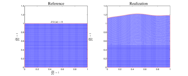
(a)                                                (b)

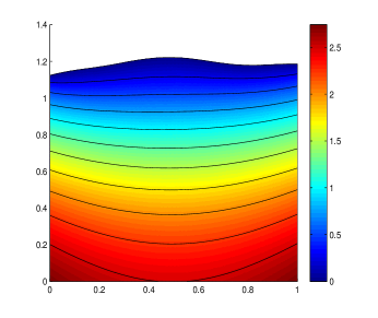
(c)

Figure 5. Stochastic deformation of a square domain and solution on a realization of the stochastic domain. (a) Reference square domain with Dirichlet boundary conditions. (b) Vertical deformation from stochastic model. (c) Contours of the solution of the parabolic PDE for $T=1$ on the stochastic deformed domain realization.

In Figure 6 (a) and (b) the normalized mean and variance errors are shown for $N_{s}=2,3,4$. Each black marker corresponds to a sparse grid level up to $w=4$. For (a) we observe a faster than polynomial convergence rate. Theoretically, the predicted convergence rate should approach sub-exponential. This is not quite clear from the graph as a higher level ($w\geq 5$) is needed to confirm the results. However, this places the simulation beyond the computational capabilities of the available hardware. In contrast, for (b), the variance error convergence rate is clearly sub-exponential, as the theory predicts.

Remark 7.

In this work for simplicity we only demonstrate the application of isotropic sparse grids to the random domain problem. However, a significant improvement in error rates can be achieved by using an anisotropic sparse grid. By adapting the number of knots across each dimension to the decay rate of $\lambda_{n}$, $n=0,1,\dots,N$ a higher convergence rate can be achieved. In particular, if the decay rate of $\lambda_{n}$ is relative fast it will be not necessary to represent all the dimensions of $\Gamma$ to high accuracy.

6.2. Truncation experiment

The truncation error with respect to $N_{s}$ is analyzed and compared with respect to $Q(\hat{u}({\bf y}))$ for $N=15$ dimensions, $k=1$ and $k=1/2$. The coefficient $c$ is changed to $1/4.35$. In Figure 7 the truncation error is plotted for (a) the mean and (b) the variance with respect to the number of truncated dimensions $N_{s}$ for the linear decay $k=1$. From these plots observe that the convergence rates are close to quadratic, which is at least one order of magnitude higher than the derived truncation convergence rate. Furthermore, in Figure 8 the mean and variance error are shown for $k=1/2$. As observed, the decay rate appears at least linear, which is at least twice the decay rate of the theoretical convergence rate. The numerical results shows that in practice a higher convergence rate is achieved than what the theory predicts.

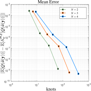
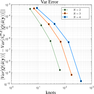
(a)	(b)

Figure 6. Isotropic sparse grid collocation convergence rates for $N=2,3,4$ with linear decay. (a) Mean error with respect to reference. Observe that the convergence rate is faster than polynomial. (b) Variance error with respect to the reference. For this case observe that the convergence rate is subexponential.

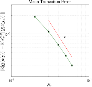
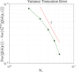
(a)	(b)

Figure 7. Truncation error with respect to the number of dimensions $N_{s}$ for linear decay $k=1$. (a) Mean error. (b) Variance error. In both cases the decay appears quadratic, which is faster than the predicted convergence rate.

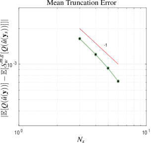
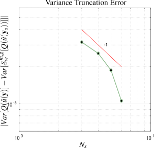
(a)	(b)

Figure 8. Truncation Error with respect to the number of dimensions $N_{s}$ for sqrt decay $k=1/2$. (a) Mean error. (b) Variance error. In both cases the decay appears at least linear.

6.3. Forcing function truncation experiment

For the last numerical experiment the decay of the forcing function truncation error (II) is tested with respect to the number of dimensions $N_{{\bf g}}$. We compare the mean and variance error of $Q({\bf g},{\bf y}_{s})$ with respect to $Q({\bf f},{\bf y}_{s})$, where

$$f({\bf x},{\bf f},{\bf y}_{s},t)=\sum_{n=1}^{N_{{\bf f}}}c_{n}(t,f_{n})\xi_{n}({\bf x},{\bf y}_{s}),\,\mbox{\&}\,f({\bf x},{\bf g},{\bf y}_{s},t)=\sum_{n=1}^{N_{{\bf g}}}c_{n}(t,f_{n})\xi_{n}({\bf x},{\bf y}_{s}),$$

${\bf x}\in{\mathcal{D}}(\omega)$ and $N_{{\bf f}}>N_{{\bf g}}$. The maps $\xi_{n}:{\mathcal{D}}(\omega)\rightarrow 1$, for $n=1,\dots,N$, are defined as

$$\xi_{n}(x_{1},x_{2}):=\exp\left(\frac{-(x_{1}-a_{n})^{2}}{\sigma}\right)\exp\left(\frac{-(x_{2}-b_{n})^{2}}{\sigma}\right),$$

where $\sigma=0.001$. The coefficients $a_{n},b_{n}\in\R$ are given such that $\xi_{n}$ are centered in a 4 by 4 grid. Let ${\bf a}:=[\frac{1}{4}\,\frac{5}{12},\,\frac{7}{12},\,\frac{3}{4}]$ $\mathbf{b}:=[\frac{5}{8}\,\frac{17}{24},\,\frac{19}{24},\,\frac{7}{8}]$, then for $i=1,\dots,4$ and $j=1,\dots,4$ let $a_{4*(i-1)+j}:={\bf a}[i]$, $b_{4*(i-1)+j}:=\mathbf{b}[j]$. Furthermore,

• For $n=1,\dots,N_{{\bf f}}$, $f_{n}$ are independent uniform distributed in $(-\sqrt{3},\sqrt{3})$, and $c_{n}(t,f_{n})=f^{2}_{n}/n$ (linear decay of the coefficients).

• The stochastic PDE is solved on the domain ${\mathcal{D}}(\omega)$ with a $513\times 513$ triangular mesh.

• $N_{{\bf f}}=12$, $N_{s}=2$, $N_{{\bf g}}=2,\dots,7$ and $c=1/4.35$.

• ${\mathbb{E}}\left[Q({\bf y}_{s},{\bf f})\right]$ and $var[Q({\bf y}_{s},{\bf f})]$ are computed with a dimensional adaptive sparse grid with $\approx$ 15,000 collocation points and a Chebyshev abscissa [15].

• ${\mathbb{E}}\left[Q({\bf y}_{s},{\bf g})\right]$ and $var[Q({\bf y}_{s},{\bf g})]$ are computed with the Clenshaw-Curtis isotropic Sparse Grid Matlab Kit [3] for $N_{{\bf g}}=2,\dots,7$.

By setting the coefficients to $c_{n}(t,f_{n})=f^{2}_{n}/n$ we have a non-linear mapping from the forcing function to the solution. From Theorem 4 the errors $|\mathbb{E}[Q(\hat{u}({\bf y}_{s},{\bf f}))]-\mathbb{E}[\mathcal{S}^{m,g}_{w}[Q(\hat{u}({\bf y}_{s},{\bf g}))]]|$ and $|Var[Q(\hat{u}({\bf y}_{s},$ ${\bf f})]-Var[\mathcal{S}^{m,g}_{w}[Q(\hat{u}({\bf y}_{s},{\bf g}))]]|$ decay as

$$\left(\sum_{n=N_{{\bf g}}+1}^{N_{{\bf f}}}{\mathbb{E}}\left[c^{2}_{n}(t,f_{n})\right]\right)^{1/2}\sim\frac{1}{N_{{\bf g}}}.$$

In Figure 9 the error of the mean and variance are plotted with respect to the number of dimensions $N_{{\bf g}}$. The error decay appears to be faster than the theoretically derived rate of $\sim 1/N_{{\bf g}}$.

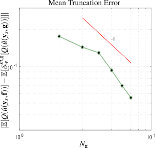
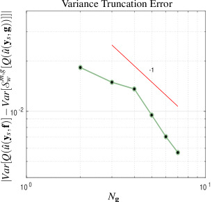
(a)	(b)

Figure 9. Forcing function truncation error with respect to the number of dimensions $N_{{\bf g}}$. The decay of the coefficients $c(t,f_{n})$, for $n=1,\dots,N_{{\bf f}}$ are set to $1/n$. The decay of the (a) Mean truncation error and the (b) Variance truncation error appears to be faster than linear.

7. Conclusions

In this paper a rigorous convergence analysis is derived for a sparse grid stochastic collocation method for the numerical solution of parabolic PDEs with random domains. The following contributions are achieved in this work:

• An analysis of the regularity of the solution with respect to the parameters describing the domain perturbation shows that an analytic extension onto a well defined region $\Theta_{\beta}\times{\color[rgb]{0,0,0}\mathscr{F}}\subset\C^{N+N_{{\bf f}}}$ exists.

• Error estimates in the energy norm for the solution and the QoI are derived for sparse grids with Clenshaw Curtis abscissas. The derived subexponential convergence rate of the sparse grid is consistent with numerical experiments.

• A truncation error with respect to the number of random variables is derived. Numerical experiments show a faster convergence rate.

This approach is well suited for a moderate number of stochastic variables, but becomes impractical for large problems with an isotropic sparse grid. However, the approach described in this paper can be easily extended to anisotropic sparse grids [37, 31]. Moreover, new approaches such as quasi-optimal sparse grids [30] are shown to have exponential convergence.

References

- [1] Robert A. Adams. Sobolev Spaces. Academic Press, 1975.
- [2] I. Babuska, F. Nobile, and R. Tempone. A stochastic collocation method for elliptic partial differential equations with random input data. SIAM Review, 52(2):317–355, 2010.
- [3] J. Bäck, F. Nobile, L. Tamellini, and R. Tempone. Stochastic spectral Galerkin and collocation methods for PDEs with random coefficients: A numerical comparison. In Jan S. Hesthaven and Einar M. Rønquist, editors, Spectral and High Order Methods for Partial Differential Equations, volume 76 of Lecture Notes in Computational Science and Engineering, pages 43–62. Springer Berlin Heidelberg, 2011.
- [4] V. Barthelmann, E. Novak, and K. Ritter. High dimensional polynomial interpolation on sparse grids. Advances in Computational Mathematics, 12:273–288, 2000.
- [5] Haim Brezis. Functional Analysis, Sobolev Spaces and Partial Differential Equations. Springer, 1st edition, November 2010.
- [6] Claudio Canuto and Tomas Kozubek. A fictitious domain approach to the numerical solution of PDEs in stochastic domains. Numerische Mathematik, 107(2):257, May 2007.
- [7] J.E. Castrillón-Candás, F. Nobile, and R. Tempone. Analytic regularity and collocation approximation for PDEs with random domain deformations. Computers and Mathematics with applications, 71(6):1173–1197, 2016.
- [8] C. Chauviere, J. S. Hesthaven, and L. Lurati. Computational modeling of uncertainty in time-domain electromagnetics. SIAM J. Sci. Comput., 28:751–775, 2006.
- [9] A. Cohen, C. Schwab, and J. Zech. Shape Holomorphy of the Stationary Navier–Stokes Equations. SIAM Journal on Mathematical Analysis, 50(2):1720–1752, 2018.
- [10] L. C. Evans. Partial Differential Equations, volume 19 of Graduate Studies in Mathematics. American Mathematical Society, Providence, Rhode Island, 1998.
- [11] H. Federer. Geometric measure theory. Grundlehren der mathematischen Wissenschaften. Springer, 1969.
- [12] D. Fransos. Stochastic Numerical Methods for Wind Engineering. PhD thesis, Politecnico di Torino, 2008.
- [13] P. Frauenfelder, C. Schwab, and R. A. Todor. Finite elements for elliptic problems with stochastic coefficients. Computer Methods in Applied Mechanics and Engineering, 194(2-5):205 – 228, 2005. Selected papers from the 11th Conference on The Mathematics of Finite Elements and Applications.
- [14] R. Gantner and M. Peters. Higher order quasi-Monte Carlo for Bayesian shape inversion. SIAM/ASA Journal on Uncertainty Quantification, 6(2):707–736, 2018.
- [15] T. Gerstner and M. Griebel. Dimension-adaptive tensor-product quadrature. Computing, 71(1):65–87, September 2003.
- [16] Diane Guignard, Fabio Nobile, and Marco Picasso. A posteriori error estimation for the steady Navier-Stokes equations in random domains. Computer Methods in Applied Mechanics and Engineering, 313:483 – 511, 2017.
- [17] R. Gunning and H. Rossi. Analytic Functions of Several Complex Variables. American Mathematical Society, 1965.
- [18] H. Harbrecht, M. Peters, and M. Siebenmorgen. Analysis of the domain mapping method for elliptic diffusion problems on random domains. Numerische Mathematik, 134(4):823–856, Dec 2016.
- [19] H. Harbrecht, R. Schneider, and C. Schwab. Sparse second moment analysis for elliptic problems in stochastic domains. Numerische Mathematik, 109:385–414, 2008.
- [20] R. Hiptmair, L. Scarabosio, C. Schillings, and Ch. Schwab. Large deformation shape uncertainty quantification in acoustic scattering. Advances in Computational Mathematics, Mar 2018.
- [21] N. Hyvönen, V. Kaarnioja, L. Mustonen, and S. Staboulis. Polynomial collocation for handling an inaccurately known measurement configuration in electrical impedance tomography. SIAM Journal on Applied Mathematics, 77(1):202–223, 2017.
- [22] I. Ipsen and R. Rehman. Perturbation bounds for determinants and characteristic polynomials. SIAM Journal on Matrix Analysis and Applications, 30(2):762–776, 2008.
- [23] Carlos Jerez-Hanckes, Christoph Schwab, and Jakob Zech. Electromagnetic wave scattering by random surfaces: Shape holomorphy. Mathematical Models and Methods in Applied Sciences, 27(12):2229–2259, 2017.
- [24] A. Klimke. Sparse Grid Interpolation Toolbox – user’s guide. Technical Report IANS report 2007/017, University of Stuttgart, 2007.
- [25] A. Klimke and B Wohlmuth. Algorithm 847: spinterp: Piecewise multilinear hierarchical sparse grid interpolation in MATLAB. ACM Transactions on Mathematical Software, 31(4), 2005.
- [26] P. Knabner and L Angermann. Discretization methods for parabolic initial boundary value problems. In Numerical Methods for Elliptic and Parabolic Partial Differential Equations, volume 44 of Texts in Applied Mathematics, pages 283–341. Springer New York, 2003.
- [27] S. G. Krantz. Function Theory of Several Complex Variables. AMS Chelsea Publishing, Providence, Rhode Island, 1992.
- [28] J.L. Lions and E. Magenes. Non-homogeneous boundary value problems and applications. Non-homogeneous Boundary Value Problems and Applications. Springer-Verlag, 1972. (3 volumes).
- [29] D. London. A note on matrices with positive definite real part. Proceedings of the American Mathematical Society, 82(3):pp. 322–324, 1981.
- [30] F. Nobile, L. Tamellini, and R. Tempone. Convergence of quasi-optimal sparse-grid approximation of Hilbert-space-valued functions: application to random elliptic pdes. Numerische Mathematik, 134(2):343–388, 2016.
- [31] F. Nobile, R. Tempone, and C. Webster. An anisotropic sparse grid stochastic collocation method for partial differential equations with random input data. SIAM Journal on Numerical Analysis, 46(5):2411–2442, 2008.
- [32] F. Nobile, R. Tempone, and C. Webster. A sparse grid stochastic collocation method for partial differential equations with random input data. SIAM Journal on Numerical Analysis, 46(5):2309–2345, 2008.
- [33] A. Nouy, A. Clément, F. Schoefs, and N. Moës. An extended stochastic finite element method for solving stochastic partial differential equations on random domains. Computer Methods in Applied Mechanics and Engineering, 197(51):4663 – 4682, 2008.
- [34] Anthony Nouy, Franck Schoefs, and Nicolas Moës. X-sfem, a computational technique based on x-fem to deal with random shapes. European Journal of Computational Mechanics, 16(2):277–293, 2007.
- [35] Stefan A. Sauter and Christoph Schwab. Boundary Element Methods, pages 183–287. Springer Berlin Heidelberg, Berlin, Heidelberg, 2011.
- [36] L. Scarabosio. Multilevel Monte Carlo on a high-dimensional parameter space for transmission problems with geometric uncertainties. ArXiv e-prints, June 2017.
- [37] Claudia Schillings and Christoph Schwab. Sparse, adaptive Smolyak quadratures for Bayesian inverse problems. Inverse Problems, 29(6):065011, 2013.
- [38] S. Smolyak. Quadrature and interpolation formulas for tensor products of certain classes of functions. Soviet Mathematics, Doklady, 4:240–243, 1963.
- [39] O. Steinbach. Numerical Approximation Methods for Elliptic Boundary Value Problems: Finite and Boundary Elements. Texts in applied mathematics. Springer New York, 2007.
- [40] D.M. Tartakovsky and D. Xiu. Stochastic analysis of transport in tubes with rough walls. Journal of Computational Physics, 217(1):248 – 259, 2006. Uncertainty Quantification in Simulation Science.
- [41] Z. Zhenhai and J. White. A fast stochastic integral equation solver for modeling the rough surface effect computer-aided design. In IEEE/ACM International Conference ICCAD-2005, pages 675–682, 2005.