Truncated Moment Problem for Dirac Mixture Densities
with Entropy Regularization

Abstract

We assume that a finite set of moments of a random vector is given. Its underlying density is unknown. An algorithm is proposed for efficiently calculating Dirac mixture densities maintaining these moments while providing a homogeneous coverage of the state space.

1 Introduction

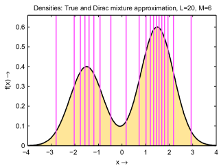
Figure 1: Maximum entropy Dirac mixture density (purple) with $20$ components and prescribed moments up to order $6$. The underlying continuous density (yellow) for generating the moments is unknown.

We consider a sequence of mappings

$$e_{k}=\int_{{\cal X}}m_{k}(\underline{x})\,\tilde{f}(\underline{x})\,d\underline{x}$$ (1)

from a Probability density function $\tilde{f}(\underline{x})$ to the so-called moments $e_{k}$ for $k=0,1,\ldots$, where ${\cal X}$ is a Polish space. Examples for ${\cal X}$ are the set of real numbers $\mathbb{R}$, the $N$-dimensional Euclidean space $\mathbb{R}^{N}$, the unit interval $[0,1]$, $\mathbb{C}$, $\mathbb{C}^{N}$, the unit circle $S^{1}=\{z\in\mathbb{C}:|z|=1\}$, and so forth. Here, we focus on the $N$-dimensional Euclidean space $\mathbb{R}^{N}$.

We are interested in the inverse problem of deducing the Probability density function $\tilde{f}(\underline{x})$ from these mapping given the moment sequence. This is called the moment problem. Here, we focus on the case that a finite moment sequence $e_{k}$ for $k=0,1,\ldots,K$ is given. The problem is then called the truncated moment problem.

Various types of moments can be considered depending upon the functions $m_{k}(\underline{x})$, $k=0,1,\ldots,K$. This includes the common power moments and trigonometric moments, which are useful for periodic state spaces such as the unit circle. Here, we focus on power moments.

We can now ask several fundamental questions such as: Does a density $\tilde{f}(\underline{x})$ exist for the given moment sequence $e_{k}$, $k=0,1,\ldots,K$? When a density $\tilde{f}(\underline{x})$ exists, is it uniquely defined by the moment sequence? When it is not uniquely defined, how is the set of densities with the given moment sequence characterized?

So far, we did not pose restrictions on the Probability density function $\tilde{f}(\underline{x})$ to be reconstructed from the moment sequence. So, $\tilde{f}(\underline{x})$ can be selected from the space of density functions, which lead to an infinite-dimensional problem. More practical questions on existence, uniqueness, and characterization can be asked, however, when we restrict ourselves to finite-dimensional approximations of the underlying true density $\tilde{f}(\underline{x})$. We consider specific densities $f(\underline{x})$ with a finite-dimensional parametrization, where we have to select a density type with a given structure. In some cases, it is also useful to consider restrictions on their parameter sets. For example, we could ask whether a Gaussian mixture density with three components exists for a given moment sequence and whether it is unique.

There are many types of parametric densities available such as Gaussian densities, Gaussian mixture densities, and exponential densities. In this paper, we consider Dirac mixture densities $f(\underline{x})$ for approximating the underlying true density $\tilde{f}(\underline{x})$.

Up to now, the only information available about the underlying true density $\tilde{f}(\underline{x})$ was the moment sequence of length $K+1$. This restricts the number of (independent) parameters of the approximating density $f(\underline{x})$ to be less than or equal to $K+1$. Restricting the number of parameters to $K+1$ is especially problematic as typically the number of available moments is itself limited. For the case of power moments of up to a certain order $M$, the number of moments quickly increases with the number of dimensions $N$ and the order $M$. Even for a moderate number of dimensions, calculating Higher-order moments becomes intractable.

A good coverage of the important regions of the state space with the approximating density $f(\underline{x})$ is mandatory in many applications. For Dirac mixture densities, this means that we need a large number of components, equivalent to a large number of parameters to be determined. When more density parameters than given moments have to be determined, we face an underdetermined inverse problem with an infinite solution set. In that case, additional information about the underlying true density $\tilde{f}(\underline{x})$ such as its support, shape, symmetries, or its smoothness is required. Alternatively, we have to directly impose additional assumptions on the approximating density $f(\underline{x})$. This information can be used to define a regularizer for picking out a single solution with the desired properties.

An interesting border case is the availability of the full underlying true density $\tilde{f}(\underline{x})$ together with a few of its moments. In that case, we want to find an approximating density $f(\underline{x})$ that maintains the given moments and is in some way as close as possible to the true density.

A detailed problem formulation is given in the following section including a compact representation of given moments up to a certain order and some words on regularization. Sec. 3 gives an overview of the state of the art.

2 Problem Formulation

A random vector $\boldsymbol{\underline{x}}=\begin{bmatrix}\boldsymbol{x}_{1},\boldsymbol{x}_{2},\ldots,\boldsymbol{x}_{N}\end{bmatrix}^{T}\in\mathbb{R}^{N}$ is characterized by a finite set of moments only. The underlying true Probability density function $\tilde{f}(\underline{x})$ of $\boldsymbol{\underline{x}}$ is unknown. The true density $\tilde{f}(\underline{x})$ can be a continuous density or a discrete density on the continuous domain $\mathbb{R}^{N}$.

Our goal is to represent the unknown Probability density function $\tilde{f}(\underline{x})$ of the random vector $\boldsymbol{\underline{x}}$ by an approximate density $f(\underline{x})$ that has the desired moments. For the approximation, we focus on discrete Probability density functions $f(\underline{x})$ on the continuous domain $\mathbb{R}^{N}$. Here, we use a so called Dirac mixture density $f(\underline{x})$ with $L$ Dirac components given by

$$f(\underline{x})=\sum_{i=1}^{L}f_{i}(\underline{x})=\sum_{i=1}^{L}w_{i}\cdot\delta(\underline{x}-\hat{\underline{x}}_{i})\enspace,$$ (2)

with positive weights, i.e., $w_{i}>0$ for $i=1,\ldots,L$, that sum up to one, i.e., $\sum_{i=1}^{L}w_{i}=1$, and locations $\hat{\underline{x}}_{i}$ with components $\hat{x}_{ki}$ for dimension $k$ with $k=1,\ldots,N$ and $\hat{\underline{x}}_{i}\neq\hat{\underline{x}}_{j}$ for $i=1,\ldots,L$, $j=1,\ldots,L$, $i\neq j$. The locations are collected in a matrix $\hat{{\mathbf{X}}}=\begin{bmatrix}\hat{\underline{x}}_{1},\hat{\underline{x}}_{2},\ldots,\hat{\underline{x}}_{L}\end{bmatrix}\in\mathbb{R}^{N\times L}$.

Our goal is to systematically find a Dirac mixture density $f(\underline{x})$ in (2) that maintains the moments of the true density $\tilde{f}(\underline{x})$ by adjusting its parameters, i.e., its weights $w_{i}$ and its locations $\hat{\underline{x}}_{i}$ for $i=1,\ldots,L$. In this paper, we focus on adjusting the locations only. The component weights are all equal. In addition, we assume that a solution exists, i.e., the number of components $L$ is selected to be large enough so that locations exist that fulfill the given moments defined in the next subsection.

We define a parameter vector $\underline{\eta}\in{\cal S}=\mathbb{R}^{L\cdot N}$ containing the parameters as

$$\underline{\eta}=\begin{bmatrix}\hat{\underline{x}}_{1}^{T},\hat{\underline{x}}_{2}^{T},\ldots,\hat{\underline{x}}_{L}^{T}\end{bmatrix}^{T}$$ (3)

and write $f(\underline{x})=f(\underline{x},\underline{\eta})$.

2.1 Given Moments

We consider power moments for characterizing the random vector $\boldsymbol{\underline{x}}$, so we will now specify concrete functions $m_{k}(\underline{x})$ in (1). For denoting the moment order, we employ a multi-index notation with $\boldsymbol{\kappa}=\begin{pmatrix}\kappa_{1},\kappa_{2},\ldots,\kappa_{N}\end{pmatrix}$ containing non-negative integer indices for every dimension. We define $|\boldsymbol{\kappa}|=\kappa_{1}+\kappa_{2}+\ldots+\kappa_{N}$, $\boldsymbol{\kappa}+i=\begin{pmatrix}\kappa_{1}+i,\kappa_{2}+i,\ldots,\kappa_{N}+i\end{pmatrix}$ with $i\in\mathbb{Z}$ such that $\boldsymbol{\kappa}+i\geq 0$, and $\underline{x}^{\boldsymbol{\kappa}}=x_{1}^{\kappa_{1}}\cdot x_{2}^{\kappa_{2}}\cdots x_{N}^{\kappa_{N}}$. For a scalar $c$, the expression $\boldsymbol{\kappa}\leq c$ is equivalent to $\kappa_{k}\leq c$ for $k=1,2,\ldots,N$. The power moments of a random vector $\underline{\boldsymbol{x}}$ with density $f(\underline{x})$ are given by

$$e_{\boldsymbol{\kappa}}=\int_{\mathbb{R}^{N}}\underline{x}^{\boldsymbol{\kappa}}f(\underline{x})\,d\underline{x}$$ (4)

for $\kappa\in\mathbb{N}_{0}^{N}$. For zero-mean random vectors $\underline{\boldsymbol{x}}$, the moments coincide with the central moments.

Moments of a certain order $m$ are given by $e_{\boldsymbol{\kappa}}$ for $|\boldsymbol{\kappa}|=m$. We define a multi-dimensional matrix ${\mathbf{E}}_{M}$ of moments of up to order $M$ as

$${\mathbf{E}}_{M}({\boldsymbol{\kappa}}+1)=\begin{cases}e_{\boldsymbol{\kappa}}&|\boldsymbol{\kappa}|\leq M\\ \text{unspecified}&\text{elsewhere}\end{cases}\enspace,$$ (5)

with $\boldsymbol{\kappa}\leq M$ and $e_{\boldsymbol{\kappa}}$ from (4). We increase the multi-index $\boldsymbol{\kappa}$ by $1$, so that the matrix ${\mathbf{E}}_{M}\in\mathbb{R}^{(M+1)\times(M+1)\times\ldots\times(M+1)}$ is indexed from $1$ to $M+1$ in every dimension.

The matrix ${\mathbf{E}}_{M}$ contains unspecified elements for $|\boldsymbol{\kappa}|\leq M$ that can either be set to zero in a full matrix or omitted in sparse matrices (when the chosen matrix implementation supports sparse matrices). With ${\cal K}_{NM}$ the set of all valid index sequences given by

$${\cal K}_{NM}=\{\kappa:|\boldsymbol{\kappa}|\leq M\}$$ (6)

the number of specified elements, i.e., the number of moments of up to order $M$, is defined as $P_{NM}=|K_{NM}|$ and is given next.

Lemma 2.1.

For an $N$-dimensional random vector, the number of moments up to order $M$ is

$$P_{NM}=\frac{(M+N)!}{M!\,N!}$$

Proof.

Elementary. ∎

For $N=10$ dimensions, the number of moments up to order $M=3$ is $P_{NM}=286$, for $M=5$ already $P_{NM}=3003$.

Of course, there is no need to specify all possible moments for $|\boldsymbol{\kappa}|\leq M$. In a practical application, there will generally be a lot more unspecified elements.

2.2 Regularization

When the length $P_{L}=L\cdot N$ of the parameter vector $\underline{\eta}$ is larger than the number of given moments, the parameters of $f(\underline{x},\underline{\eta})$ are redundant and a regularizer for $f(\underline{x},\underline{\eta})$ is required. Here, regularization is performed by selecting the least informative Dirac mixture, e.g., the one having maximum entropy. As the Shannon entropy for Dirac mixture densitys is not well defined, we use the entropy of a corresponding Piecewise constant density. This results in a constrained optimization problem, where the most homogeneous Dirac mixture approximation $f(\underline{x},\underline{\eta})$ is desired that fulfills the given moments and maximizes the entropy.

3 State of the Art

For determining $P_{L}$ parameters of a Dirac mixture density in (2) from a set of $P_{NM}$ moments, we have to distinguish three cases:

1. $P_{L}<P_{NM}$, the overdetermined case, i.e., the number of parameters is smaller than the number of moments.

2. $P_{L}=P_{NM}$, the fully determined case, i.e., the number of parameters is equal to the number of moments.

3. $P_{L}>P_{NM}$, the underdetermined case, i.e., the number of parameters is larger than the number of moments.

3.1 $P_{L}<P_{NM}$, the Overdetermined Case

For the overdetermined case, no literature seems to be available. This case is interesting from a theoretical point of view and it will be discussed in more detail later in this paper. From a practical point of view, it makes sense when for some reason the redundancy in the moments can be used to better estimate the parameters of the desired Dirac mixture density. On the other hand, as discussed above, many Dirac components are required to cover the interesting parts of the state space, which leads to a large amount of parameters. It might then be impractical to calculate more moments than parameters.

3.2 $P_{L}=P_{NM}$, the Fully Determined Case

The fully determined case has been treated a lot in literature in the context of nonlinear Kalman filtering. Moment-based approximations of Gaussian densities are the basis for Linear Regression Kalman Filters (LRKFs) lefebvre_linear_2005 . Examples are the Unscented Kalman Filter (UKF) in julier_new_2000 and its scaled version in julier_scaled_2002 .

The case of maintaining the first two moments received most attention. Moments of up to second order can be maintained by a Dirac mixture density with two Dirac components per dimension with an optional additional point placed at the mean. This has the huge advantage that the number of components only grows linearly with the number of dimensions.

Maintaining Higher-order moments is important for two reasons: First, even for Gaussian densities, it makes sense to explicitly consider the Higher-order moments as the simplest Dirac mixture (the one with two points per dimension) does not possess the same Higher-order moments as a Gaussian density. Second, for non-Gaussian densities Higher-order moments are essential for capturing asymmetry, multimodality, and so forth.

Third-order moments are considered in julier_reduced_2002 . A Dirac mixture density with $2N+2$ weighted components is designed that maintains moments of up to second order and, in addition, minimizes the third-order moments. Minimizing the third-order moments is motivated by an underlying Gaussian density, but is not useful for general densities, where asymmetries can lead to nonzero third-order moments.

Under several strong assumptions, Dirac mixture densities with prescribed higher-order moments have been derived in tenne_higher_2003 . Assumptions include a placement of components on the coordinate axes only and symmetric densities, so that all odd moments are set to zero. For the actual derivations, Gaussian densitys were assumed and the point sets were limited to $4N+1$ and $6N+1$ samples with $N$ the number of dimensions.

straka_measures_2014 proposes two methods for constructing scalar Dirac mixture densities with arbitrary first three moments. The first method is a direct approach based on solving for the parameters of a Dirac mixture density with three weighted components given the first three moments under certain symmetry conditions. Existence of a solution is not guaranteed. The second method is an indirect approach, where a Gaussian mixture density with two components is matched to the given moments, where two degrees of freedom remain to be set by the user. In a second step, two Dirac mixture densities with three components are calculated matching the first two moments of the individual Gaussian components of the Gaussian mixture density. This results in a final Dirac mixture density with six components matching the given three moments.

Dirac mixture approximation of Circular probability density functions analogous to the UKF for linear quantities is introduced in ACC13_Kurz for the Von Mises distribution and the Wrapped Normal distribution. Based on a closed-form expression for matching the first Circular moment, three Dirac components are systematically placed by exploiting symmetry. In Fusion14_KurzGilitschenski , a closed-form solution is derived for a symmetric wrapped Dirac mixture density with five components based on matching the first two circular moments. This Dirac mixture approximation of continuous Circular probability density functions has already been applied to sensor scheduling based on bearings-only measurements Fusion13_Gilitschenski . The results have also been used to perform recursive circular filtering for tracking an object constrained to an arbitrary one-dimensional manifold in IPIN13_Kurz .

3.3 $P_{L}>P_{NM}$, the Underdetermined Case

We will now consider the case of more parameters than given moments. As the solution of this inverse problem is not unique, it either requires more information about the underlying density to be reconstructed or assumptions on the desired Dirac mixture density. In either case, we will perform regularization to guarantee a unique solution with the desired properties. We will consider prior information in two different ways: Either the full density is given or we just know that the underlying true density is smooth.

3.3.1 Full Density Available

When the full underlying true density is given, the most basic problem is to not maintain any moment. Regularization is performed by minimizing a distance between the underlying true density and its Dirac mixture approximation. As distances between continuous densities and discrete densities on continuous domains are difficult to define, the densities are typically transformed to a different representation before the distance computation is performed.

Methods for Dirac mixture approximation of scalar continuous densities based on a distance between cumulative distributions with no moment constraint are introduced in CDC06_Schrempf-DiracMixt ; MFI06_Schrempf-CramerMises for a given but arbitrary number of components. An algorithm for sequentially increasing the number of components is given in CDC07_HanebeckSchrempf and applied to recursive nonlinear prediction in ACC07_Schrempf-DiracMixt .

For arbitrary multi-dimensional Gaussian densities, Dirac mixture approximations are systematically calculated in CDC09_HanebeckHuber . The comparison of densities is performed by comparing probability masses under kernels of arbitrary location and size. For this purpose, the so called Localized Cumulative Distribution (LCD) is introduced in MFI08_Hanebeck-LCD . A modified Cramér-von Mises distance is then defined based on the LCDs. For the case of standard normal distributions with a subsequent transformation, a more efficient method is given in ACC13_Gilitschenski .

For multidimensional densities with given mean and given variances in every dimension, a method for placing an arbitrary number of Dirac components along the coordinate axes is introduced in IFAC08_Huber . The multi-dimensional problem is broken down into one-dimensional problems that are solved by minimizing the distance between cumulative distributions given the two moment constraints.

Multidimensional Dirac mixture approximations of arbitrary densities with an arbitrary component placement and arbitrary higher-order moment constraints are calculated in CISS14_Hanebeck . Compared to CDC09_HanebeckHuber , a faster but suboptimal distance comparison is used. Instead of comparing the probability masses on all scales as in CDC09_HanebeckHuber , repulsion kernels are introduced to assemble an Induced kernel density and perform the comparison of the true density with its Dirac mixture approximation. This method is adapted to Gaussian densities in Fusion14_Hanebeck , where a closed-form expression for the distance measure is derived. In addition, a randomized optimization method is employed instead of a quasi-Newton method. This has the advantage of being easier to implement with only a slight decrease in performance. An approach similar to the one proposed in CISS14_Hanebeck has been derived for Dirac mixture approximation of Circular probability density functions with an arbitrary number of Dirac components in IFAC14_Hanebeck .

3.3.2 Smoothness Constraint

When it is only known that the underlying density is a smooth continuous density, the first idea that might come to mind is to use an indirect approach. In a first step, a continuous density with the desired moments is found. This can be any smooth parametric density from the exponential family or from a mixture family such as a Gaussian mixture density. In a second step, a Dirac mixture approximation of this continuous density is performed. This Dirac mixture approximation can be performed with methods discussed before that calculate the Dirac mixture closest to the given density while simultaneously maintaining the given moments.

The indirect approach has several disadvantages. It is difficult to take care of the given smoothness condition by finding a parametric continuous density first as this includes finding both an appropriate type of density with an appropriate structure and appropriate parameters. This step will most likely introduce unwanted artifacts. In addition, the approximation becomes unnecessarily complicated as we now have to solve two moment problems, a moment problem for the continuous density in the first step and a moment problem for its Dirac mixture approximation in the second step.

We prefer a direct approach, where the smoothness constraint is fulfilled by finding the most homogeneously distibuted Dirac mixture approximation under the given moment constraints. To the author’s knowledge, no solution to this problem exists for the case of multi-dimensional densities with an arbitrary placement of Dirac components.

3.4 Contribution of this Paper

We consider the finite moment problem of calculating parameters of a Dirac mixture density with a given number of components and prescribed moments. The true underlying density is unknown. We focus on redundant problems, where the number of parameters is (much) larger than the number of given moment constraints. This is an underdetermined problem with an infinite solution set, so that a regularizer is required to exploit redundancy. Here, we desire a Dirac mixture density with the most homogeneous coverage under the given moment constraints.

For regularization, the entropy of the Dirac mixture density could be used. However, the Shannon entropy is not well defined for discrete densities on continuous domains. Here, we propose to use the entropy of the corresponding maximum entropy piecewise constant density approximation. This approximation has a nice interpretation and, for given Dirac components, is given as the solution of a convex optimization problem with linear inequality constraints. Regularization is now performed by selecting the components of the Dirac mixture density in such a way that the entropy of this Piecewise constant density approximation is maximized.

The remainder of this paper is structured as follows. The Piecewise constant density used for guaranteeing a homogeneous coverage of the final Dirac mixture density is introduced in Sec. 4. Calculating the Dirac mixture density with given moments and homogeneous coverage is discussed in Sec. 5. Implementation details are given in Sec. 6. An evaluation is conducted in Sec. 7. Conclusions are drawn in Sec. 8.

4 Piecewise Constant Density Approximation

In this section, we derive a piecewise constant approximation of the given Dirac mixture. Its parameters are calculated in such a way that the Shannon entropy is maximized. We now define the specific form of piecewise constant density used in this paper.

Definition 4.1 (Piecewise constant density).

We define a piecewise constant density as a mixture with $L$ components

$$p(\underline{x})=\sum_{i=1}^{L}R(\underline{x},\hat{\underline{x}}_{i},d_{i})\enspace,$$

where each component $R(\underline{x},\hat{\underline{x}}_{i},d_{i})$, $i=1,\ldots,L$ is constant within a sphere of radius $d_{i}$ and given by

$$R(\underline{x},\hat{\underline{x}}_{i},d_{i})=\begin{cases}h_{i}&\text{for }\|\underline{x}-\hat{\underline{x}}_{i}\|\leq d_{i}\\ 0&\text{elsewhere}\end{cases}\enspace,$$

with $d_{i}>0$ and the constant heights $h_{i}$ for each component to be determined. In addition, we desire that the components are disjoint according to

$$d_{i}+d_{j}<\|\hat{\underline{x}}_{i}-\hat{\underline{x}}_{j}\|$$ (7)

holds for all $i=1,\ldots,L$, $j=1,\ldots,L$ with $i\neq j$.

Remark 4.1.

The diameters $d_{i}$, $i=1,\ldots,L$ will be collected in a vector $\underline{d}=\begin{bmatrix}d_{1},\ldots,d_{L}\end{bmatrix}^{T}$.

Remark 4.2.

By exploiting symmetry, (7) needs to be checked only for $i=1,\ldots,L-1$, $j=i+1,\ldots,L$. This results in a total of $(L+1)L/2$ inequality constraints.

When the piecewise constant density is used as a representation of a given Dirac mixture with weights $w_{i}$, $i=1,\ldots,L$, we can calculate appropriate values for the constant heights $h_{i}$.

Lemma 4.1.

The constant height for each component $h_{i}$, $i=1,\ldots,L$ is given by

$$h_{i}=\frac{w_{i}}{V_{N}(d_{i})}\enspace.$$

with $V_{N}(.)$ the volume of an $N$-dimensional hyper-sphere given by

$$V_{N}(d)=\frac{\pi^{\frac{N}{2}}}{\Gamma\left(\frac{N}{2}+1\right)}\,d^{N}\enspace.$$

Proof.

As the components of the piecewise constant density $p(\underline{x})$ according to Definition 4.1 are disjoint, it is possible to treat the individual components separately. We require that the probability mass of the individual component $i$ is equal to the mass of the corresponding Dirac component, which is written as

$$\int_{\mathbb{R}^{N}}R(\underline{x},\hat{\underline{x}}_{i},d_{i})\,d\,\underline{x}=w_{i}\enspace.$$

By evaluating the left-hand-side, we obtain an integral over the $N$-dimensional hyper-sphere ${\cal S}_{N}(d_{i})$ with radius $d_{i}$ as

$$\begin{split}\int_{{\cal S}_{N}(d_{i})}R(\underline{x},\hat{\underline{x}}_{i},d_{i})\,d\,\underline{x}&=\int_{{\cal S}_{N}(d_{i})}h_{i}\,d\,\underline{x}\\ &=h_{i}\int_{{\cal S}_{N}(d_{i})}\,d\,\underline{x}\\ &=h_{i}\cdot V_{N}(d_{i})=w_{i}\enspace,\end{split}$$

which concludes the proof. ∎

We are now interested in piecewise constant densities that are as homogeneously distributed as possible under certain constraints. For that purpose, we will maximize its Shannon entropy.

Lemma 4.2.

The Shannon entropy $h(p)$ of the piecewise constant density $p(.)$ defined in Definition 4.1 is given by

$$h(p)=c_{N}-\sum_{i=1}^{L}w_{i}\log\left(\frac{w_{i}}{d_{i}^{N}}\right)\enspace,$$

where $c_{N}$ is a constant depending on the number of dimensions $N$.

Proof.

The Shannon entropy of the Piecewise constant density $p(\underline{x})$ according to Definition 4.1 is defined as

$$h(p)=E\left\{-\log(p)\right\}=-\int_{\mathbb{R}^{N}}p(\underline{x})\log\left(p(\underline{x})\right)\,d\,\underline{x}\enspace.$$

Again, as the components of the Piecewise constant density $p(\underline{x})$ are disjoint, we can exchange summation and integration, which gives

$$h(p)=-\sum_{i=1}^{L}\int_{\mathbb{R}^{N}}R(\underline{x},\hat{\underline{x}}_{i},d_{i})\log\left(R(\underline{x},\hat{\underline{x}}_{i},d_{i})\right)\,d\,\underline{x}$$

or

$$\begin{split}h(p)&=-\sum_{i=1}^{L}\int_{{\cal S}_{N}}R(\underline{x},\hat{\underline{x}}_{i},d_{i})\log\left(R(\underline{x},\hat{\underline{x}}_{i},d_{i})\right)\,d\,\underline{x}\\ &=-\sum_{i=1}^{L}\int_{{\cal S}_{N}}h_{i}\log(h_{i})\,d\,\underline{x}\\ &=-\sum_{i=1}^{L}h_{i}\log(h_{i})\underbrace{\int_{{\cal S}_{N}(d_{i})}\,d\,\underline{x}}_{V_{N}(d_{i})}\enspace.\end{split}$$

With $h_{i}$ from Lemma 4.1, we obtain

$$\begin{split}h(p)&=-\sum_{i=1}^{L}w_{i}\log\left(\frac{w_{i}}{V_{N}(d_{i})}\right)\\ &=\sum_{i=1}^{L}w_{i}\left[\log\left(\frac{\pi^{\frac{N}{2}}}{\Gamma\left(\frac{N}{2}+1\right)}\right)-\log\left(\frac{w_{i}}{d_{i}^{N}}\right)\right]\\ &=\log\left(\frac{\pi^{\frac{N}{2}}}{\Gamma\left(\frac{N}{2}+1\right)}\right)-\sum_{i=1}^{L}w_{i}\log\left(\frac{w_{i}}{d_{i}^{N}}\right)\enspace,\end{split}$$

which gives the desired result. ∎

Lemma 4.3.

For a given Dirac mixture according to (2) with weights $w_{i}$ and components $\hat{\underline{x}}_{i}$, $i=1,\ldots,L$, the corresponding maximum entropy Piecewise constant density in Definition 4.1 is the solution to the optimization problem

$$\begin{array}[]{llclll}\underline{d}=\displaystyle\operatorname*{arg\,max}_{\underline{d}}\left(h\left(p(\underline{\eta},\underline{d})\right)\right)&&&&&\\ &\text{ s.t. }&d_{i}>0&\text{for}&i=1,\ldots,L&\\[5.69054pt] &&\hbox{\multirowsetup$d_{i}+d_{j}<\|\hat{\underline{x}}_{i}-\hat{\underline{x}}_{j}\|$}&\hbox{\multirowsetup for}&i=1,\ldots,L&\hbox{\multirowsetup with $i\neq j$ \enspace.}\\ &&&&j=1,\ldots,L&\end{array}$$

Remark 4.3.

The optimization (maximization) problem in Lemma 4.3 is characterized by a concave objective function as

$$\frac{\partial h\left(p(\underline{\eta},\underline{d})\right)}{\partial d_{i}}=-N\frac{w_{i}}{d_{i}}$$

for $i=1,\ldots,L$ and subject to linear inequality constraints. It remains to be investigated whether the inequality constraints form a convex set, which would make the optimization problem convex.

Remark 4.4.

In general, the optimization problem in Lemma 4.3 requires a total of $L(L+1)/2$ linear inequality constraints: $d_{i}>0$ for $i=1,\ldots,L$, which gives $L$ inequality constraints, and $d_{i}+d_{j}<\|\hat{\underline{x}}_{i}-\hat{\underline{x}}_{j}\|$ for $i=1,\ldots,L$, $j=1,\ldots,L$, and $i\neq j$, which together with symmetry gives another $L(L-1)/2$ inequalities. The scalar case $N=1$ is an exception as the positions $\hat{x}_{i}$, $i=1,\ldots,L$ can be ordered. In that case, we have a total of $2L-1$ linear inequality constraints: $d_{i}>0$ for $i=1,\ldots,L$ and $\hat{x}_{i}+d_{i}<\hat{x}_{i+1}-d_{i+1}$ for $i=1,\ldots,L-1$.

5 Homogeneous Dirac Mixture Approximation with Given Moments

Our goal is an algorithm for the efficient calculation of a Dirac mixture density with given moments and a homogeneous coverage of the state space. We will start with taking a look at the given moments. They will act as constraints for the desired Dirac mixture density.

Given moments up to an order $M$ are stored in the matrix ${\mathbf{E}}_{M}$ from (5). These given moments will be denoted as $\tilde{{\mathbf{E}}}_{M}$. The actual moments of the Dirac mixture density in (2) are just denoted by ${\mathbf{E}}_{M}$, so that our moment constraints can be written as

$${\mathbf{E}}_{M}\stackrel{{\scriptstyle!}}{{=}}\tilde{{\mathbf{E}}}_{M}\enspace,$$

where the left hand side depends on $\underline{\eta}$, i.e., we have ${\mathbf{E}}_{M}={\mathbf{E}}_{M}(\underline{\eta})$.

Depending on the number of given moments compared to the number of parameters of the desired Dirac mixture density, we have to distinguish between three different cases:

Case 1:

In the first case, the number of given moments is larger than the number of parameters. Now, the system of nonlinear equations given by

$${\mathbf{E}}_{M}(\underline{\eta})-\tilde{{\mathbf{E}}}_{M}\stackrel{{\scriptstyle!}}{{=}}0$$

is overdetermined as it has more equations than unknowns, i.e., number of parameters or length of the parameter vector $\underline{\eta}$. In that case, we can calculate a least-squares solution as

$$\underline{\eta}=\operatorname*{arg\,max}_{\underline{\eta}\in{\cal S}}\left\|\tilde{{\mathbf{E}}}_{M}-{\mathbf{E}}_{M}\right\|_{F}^{2}\enspace,$$

where $\|.\|_{F}$ is the Frobenius norm defined for a matrix ${\mathbf{H}}\in\mathbb{R}^{M_{1}\times M_{2}}$ with elements $h_{ij}$, $i=1,\ldots,M_{1}$, $j=1,\ldots,M_{2}$ as

$$\|{\mathbf{H}}\|_{F}=\sqrt{\sum_{i=1}^{M_{1}}\sum_{j=1}^{M_{2}}|h_{ij}|^{2}}\enspace.$$

A generalization would be to introduce weighting factors for moments of different orders.

Case 2:

In the second case, the number of given moments is exactly equal to the number of parameters. In this case, we have to solve the system of nonlinear equations given by

$${\mathbf{E}}_{M}(\underline{\eta})-\tilde{{\mathbf{E}}}_{M}\stackrel{{\scriptstyle!}}{{=}}0\enspace.$$

for the parameter vector $\underline{\eta}$. In the case of power moments, the left hand side leads to a system of multi-dimensional higher-order polynomials. Analytic solutions are only available in rare special cases, so that numerical root-finding technqies have to be applied. In addition, the solution is not necessarily unique.

Case 3:

The third and last case is the one that we will pursue further. Here, the number of moment constraints is smaller than the number of parameters, so calculating the desired Dirac mixture density is underdetermined. Just considering the moment constraints would give an infinite solution set for the desired parameter vector $\underline{\eta}$.

We will now pursue the third case. In that case, the solution, the parameter vector of the Dirac mixture density with the desired moments, is underdetermined. Thus, we have redundancy available that can be exploited, so that we can impose additional constraints on the desired Dirac mixture density to perform a regularization and to finally end up with a unique solution.

Here, we want the final Dirac mixture density to be not more informative as already specified by the given moments: It should be as uninformative as possible within the given moment constraints. The density in a Dirac mixture is encoded by both the weights and the “density” of its components, that is their relative spacing. When we do not want to favor certain regions of the state space in terms of their density, the Dirac mixture should be as homogeneous as possible in terms of weight distribution and location distribution. Intuitively, for equally weighted components we somehow desire equal distances between neighboring components or equivalently equal free spaces around each component. As this is not very precise and does not hold for unequally weighted components, we need a formal definition of homogeneity.

As a convenient, effective, and intuitive regularizer we use the corresponding Piecewise constant density for a Dirac mixture density as introduced in Sec. 4. The most homogenous Dirac mixture from the infinite solution set then is defined as the one that maximizes the entropy of the corresponding Piecewise constant density.

For performing the optimization, we again couple the Piecewise constant density with the Dirac mixture in such a way that the locations $\hat{\underline{x}}_{i}$ of the Dirac mixture are the midpoints of the spherical support for each component of the Piecewise constant density. The probability mass $w_{i}$ of the Dirac mixture determines the height $h_{i}$ of each component of the Piecewise constant density. In contrast to Sec. 4, now both the diameters $d_{i}$ and the locations $\hat{\underline{x}}_{i}$ are variables that are simultaneously optimized. The optimization result provides the locations $\hat{\underline{x}}_{i}$ of the most homogenous Dirac mixture. The optimal diameters $d_{i}$ of the maximum entropy Piecewise constant density are a by-product and can be used for visualization.

Theorem 5.1.

For given moments collected in the moment matrix $\tilde{{\mathbf{E}}}_{M}$, a Dirac mixture density with the same moments and a corresponding maximum entropy Piecewise constant density is the solution to the optimization problem

$$\begin{array}[]{llclll}[\underline{\eta},\underline{d}]=\displaystyle\operatorname*{arg\,max}_{\underline{\eta},\underline{d}}\left(h\left(p(\underline{\eta},\underline{d})\right)\right)&&&&&\\ &\text{ s.t. }&{\mathbf{E}}_{M}=\tilde{{\mathbf{E}}}_{M}&&&\\[5.69054pt] &&d_{i}>0&\text{for}&i=1,\ldots,L&\\[5.69054pt] &&\hbox{\multirowsetup$d_{i}+d_{j}-\|\hat{\underline{x}}_{i}-\hat{\underline{x}}_{j}\|<0$}&\hbox{\multirowsetup for}&i=1,\ldots,L&\hbox{\multirowsetup with $i\neq j$ \enspace.}\\ &&&&j=1,\ldots,L&\end{array}$$

Of course, compared to the sole optimization of the diameters of the Piecewise constant density in Sec. 4, this optimization problem now has nonlinear constraints: The equality constraints for maintaining the desired moments are typically nonlinear. Also the inequality constraints for avoiding collisions of the spherical supports of the Piecewise constant densities are now nonlinear as the locations $\hat{\underline{x}}_{i}$ now are variables.

Remark 5.1.

It is important to note that all the required statistics such as the moments are directly calculated from the Dirac mixture. They are not calculated from the corresponding Piecewise constant density as this one solely serves regularization purposes.

6 Implementation and Complexity

Given the algorithm derived in the previous section, our goal is the efficient calculation of a Dirac mixture density with given moments and a homogeneous coverage of the state space. Homogeneity is achieved by a regularizer that picks out the most homogeneous solution from the infinite solution set that we have in case of more parameters than moment constraint.

6.1 Symmetric Densities

Often, more information besides the moments is available about the true density $\tilde{f}(\underline{x})$, such as information on its support or on given symmetries. Even when information of this type is unavailable, analogous assumptions could be made about the approximating density $f(\underline{x})$.

Here, we consider a special case of symmetric densities, Dirac mixture densities $f(\underline{x})$ that are symmetric with respect to their expected value $\operatorname{E}_{f}\left\{\underline{x}\right\}$. We only have to specify $L$ master components $f_{1},\ldots,f_{L}$ and implicitly end up with $2L$ components, i.e., $f_{1},\ldots,f_{2L}$, where the master components $f_{1},\ldots,f_{L}$ control slave components $f_{L+1},\ldots,f_{2L}$. The slave components are symmetric copies of the master components in the sense, that

$$\hat{\underline{x}}_{i+L}-\operatorname{E}_{f}\left\{\underline{x}\right\}=-(\hat{\underline{x}}_{i}-\operatorname{E}_{f}\left\{\underline{x}\right\})$$

holds for $i=1,\ldots,L$. The weights $w_{i}$ and the diameters $d_{i}$ are simply copied according to $w_{i+L}=w_{i}$ and $d_{i+L}=d_{i}$ for $i=1,\ldots,L$.

Exploiting symmetries in this form has two major advantages. First, complexity is reduced as only half as many variables have to be optimized (this does not depend upon the number of dimensions). Second, the prescribed expected value is automatically maintained without an explicit constraint.

Remark 6.1.

The master components are not confined to specific parts of the state space. They can be located anywhere, which simplifies the implementation.

6.2 Complexity

Regularization is performed by maximizing the Shannon entropy of the corresponding Piecewise constant density, which requires complying with a number of constraints quadratic in the number of Dirac components. We will now take a look at the complexity, especially the number of constraints to maintain. The number of equality constraints (the moment constraints) is prespecified and for a given order $M$ bounded by (6). For the inequality constraints, we have $L$ linear positivity constraints for the radii $d_{i}$, $i=1,\ldots,L$ of the Piecewise constant density and $(L-1)L/2$ nonlinear collision constraints. The latter ones are the most critical and will be investigated further, where we distinguish the scalar or $1$-dimensional case and the $N$-dimensional case with $N>1$.

In the scalar case, the number of collision constraints is reduced by maintaining an ordered list of Dirac components. Then, only the distances between neighbors have to be considered, which reduces the number of collision constraints from $(L-1)L/2$ to $L-1$.

For the general multi-dimensional case with $N>1$, the number of collision constraints does not depend upon the dimension. However, it depends quadratically upon the number of components. For a small number of components, say up to $20$, this poses no problem. For more components, however, the number of constraints needs to be reduced.

Reducing the number of collision constraints while still guaranteeing a correct solution will be pursued in a follow-up paper. The key is to exploit the fact that simpler constraints can be devised to check for collisions of the support spheres onto the coordinate axes. This is much simpler and leads to fewer constraints. Non-colliding projections are a sufficient, but not a necessary, condition for non-colliding supports. Based on this insight, expensive collision constraints have to be considered for far fewer components. Details are given in the conclusions.

7 Evaluation

We will now demonstrate the performance of the proposed Dirac mixture approximation method by some examples. One-dimensional and two-dimensional densities will be considered.

Remark 7.1.

It is important to note, that in all cases where we consider underlying continuous densities, these are only used for generating the moments. They are not known to the approximation methods!

For comparison, we employ a solver that directly finds a root of the underdetermined system of equations given by the moment constraints. We use a Levenberg-Marquardt method for that purpose, that we from now on call Levenberg-Marquardt Dirac mixture approximation method. Matlab provides an implementation by calling fsolve with the appropriate options. This solver does neither provide unique nor reproducible results.

In the simulations, both optimization methods, the Levenberg-Marquardt Dirac mixture approximation method and the proposed Maximum entropy Dirac mixture approximation method, are initialized with a random parameter vector $\underline{\eta}$ drawn from a standard normal distribution.

7.1 Examples for the One-dimensional Case

We begin with the simplest case of generating moments from a Gaussian density that are then used for characterizing a Dirac mixture density. For a standard normal distribution, we calculate the first two moments $e_{1}$, $e_{2}$. Then, we employ the Levenberg-Marquardt Dirac mixture approximation method and the Maximum entropy Dirac mixture approximation method to find Dirac mixture densities with $L=6$ components having exactly these moments. A comparison of densities and distributions is shown in Fig. 2, where the top two figures show the result of the Levenberg-Marquardt Dirac mixture approximation. This is just one representative result, as the solution is not unique and changes for every optimization performed. The bottom row in Fig. 2 shows the result of the Maximum entropy Dirac mixture approximation. Here, the coverage is much more homogeneous. In addition, it becomes clear that it comes close to the underlying Gaussian as a maximum entropy solution is considered and the Gaussian is the continuous density with the highest entropy given a certain variance. This convergence becomes even clearer when taking a look at Fig. 3. When the number of Dirac components increases, in that case to $L=10$ and $L=15$, the generated Dirac mixture converges to the underlying Gaussian although this density is not known to the algorithm.

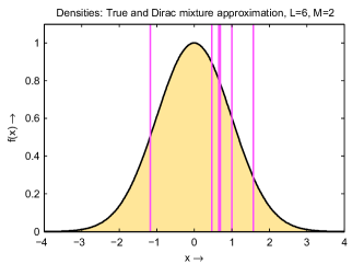
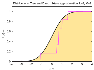
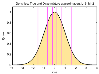
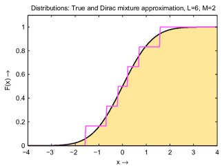
Figure 2: Comparison of two Dirac mixture approximation methods for an underlying Gaussian density. (Top row) Result of solving the underdetermined moment constraints with the Levenberg-Marquardt Dirac mixture approximation method. (Bottom row) Result of the proposed Maximum entropy Dirac mixture approximation method. (Left column) Comparison of the densities, where the (unknown) underlying Gaussian densities are shown in yellow and the Dirac mixture densities in purple. (Right column) Comparison of the cumulative distributions, where the (unknown) underlying Gaussian distribution is shown in yellow and the distributions of the Dirac mixtures in purple.

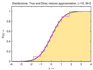
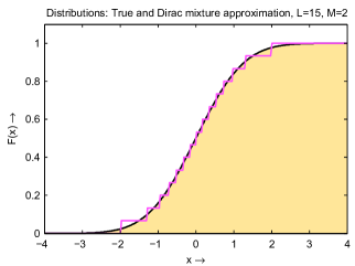
Figure 3: Dirac mixture approximation for an underlying Gaussian density with an increasing number of components $L$. Only moments up to order $M=2$ are maintained. (left) $L=10$. (Right) $L=15$. The Dirac mixture density quickly approaches the underlying Gaussian, although this density is not known to the approximation method.

A similar evaluation is now performed by using moments obtained from a Gaussian mixture density with two components, weights $w_{1}=0.4$, $w_{2}=0.6$, means $m_{1}=-1.5$, $m_{1}=1.5$, and standard deviations $\sigma_{1}=\sigma_{2}=0.7$. Moments $e_{0}=1,e_{1},\ldots,e_{4}$ up to fourth order are calculated according to the appendix and used for generating a Dirac mixture with these moments. Fig. 4 shows the results for $L=10$ components, where the top row shows a comparison of densities and distributions for Dirac mixtures obtained with Levenberg-Marquardt Dirac mixture approximation. Again, this is only one possible result as the solution is not unique. The bottom row shows the result obtained with Maximum entropy Dirac mixture approximation, which is very homogeneous and close to the underlying Gaussian mixture density in terms of its distribution.

Fig. 5 then shows that, for $M=6$ moments, the Maximum entropy Dirac mixture approximation quickly converges to the underlying Gaussian mixture density as demonstrated for $L=15$ and $L=25$.

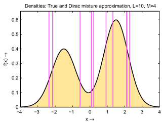
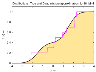
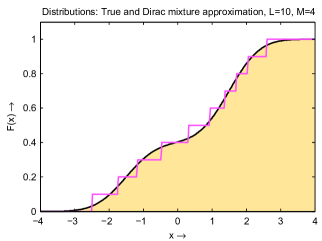
Figure 4: Comparison of two Dirac mixture approximation methods for an underlying Gaussian mixture density. (Top row) Result of solving the underdetermined moment constraints with the Levenberg-Marquardt Dirac mixture approximation method. (Bottom row) Result of the proposed Maximum entropy Dirac mixture approximation method. (Left column) Comparison of the densities, where the (unknown) underlying Gaussian mixture densities are shown in yellow and the Dirac mixture densities in purple. (Right column) Comparison of the cumulative distributions, where the (unknown) underlying Gaussian mixture distributions are shown in yellow and the distributions of the Dirac mixtures in purple. In both cases, moments up to order $M=4$ are maintained and the Dirac mixture comprises $L=10$ components.

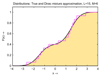
Figure 5: Dirac mixture approximation for an underlying Gaussian mixture density with an increasing number of components $L$. Moments up to order $M=6$ are maintained. (left) $L=15$. (Right) $L=25$. The Dirac mixture density quickly approaches the underlying Gaussian mixture, although this density is not know to the approximation method.

7.2 Examples for the Two-dimensional Case

For the two-dimensional case $N=2$, we consider Dirac mixture densities maintaining moments up to second order, i.e., $e_{00}=1$ (the normalization constant), $e_{01}$, $e_{10}$, $e_{11}$, $e_{02}$, and $e_{20}$ are prespecified. For the specific choice of moments corresponding to the axis-aligned normal distribution $e_{00}=1$, $e_{01}=0$, $e_{10}=0$, $e_{11}=0$, $e_{02}=3$, and $e_{20}=1$, we obtain the results shown in Fig. 6. Here, symmetry is enforced as introduced in Subsec. 6.1. As a result, only $20$ master components are optimized and $20$ slave components follow accordingly.

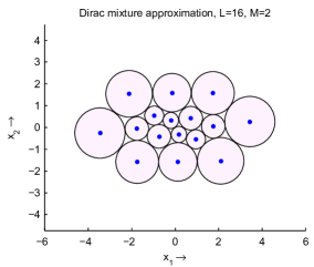
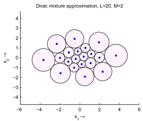
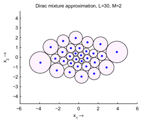
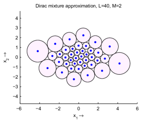
Figure 6: Plots of Dirac mixture densities maintaining moments up to second order $M=2$ with different numbers of components. (top left) $L=16$. (top right) $L=20$. (bottom left) $L=30$. (bottom right) $L=40$. Symmetry is enforced, so that only $20$ master components are optimized.

It is obvious from Fig. 6 that the resulting Dirac mixture densities converge to a Gaussian density with the given moments when the number of components increases. Again, the underlying density shape, in this case the Gaussian, is not known to the Dirac mixture approximation method.

8 Conclusion

This paper provides an efficient algorithm for calculating Dirac mixture densities with given moments and a homogeneous coverage of the state space. We focus on the case of fewer moment constraints than parameters. Ensuring a unique solution and exploiting the redundancy by optimizing the component arrangement is performed by regularization with respect to a corresponding Piecewise constant density. The most homogeneous Dirac mixture density is obtained by maximizing the entropy of this Piecewise constant density.

8.1 Applications

The proposed Maximum entropy Dirac mixture approximation method will be used for generalizing the Progressive Gaussian Filter introduced for generative system models in Fusion13_Hanebeck and for systems with given likelihoods in Fusion14_Steinbring . So far, the Progressive Gaussian Filter maintains moments up to second order when progressively performing a measurement update. In addition, a Gaussian assumption is made. Using the proposed Maximum entropy Dirac mixture approximation, higher-order moments will be propagated without any density assumption.

The Piecewise constant density for a given Dirac mixture density as derived in Sec. 4 might also be useful by itself in other contexts than providing a convenient density for plug-in estimation of the entropy of a Dirac mixture density.

8.2 Extensions

Now, we will discuss several extensions to the basic algorithm described in this paper. First, we discuss optimizing the weights in addition to the locations of the components of the considered Dirac mixture density. Second, we focus on the complexity and how to decrease it. Third, we consider spaces different from the Euclidean space $\mathbb{R}^{N}$.

Weights

In this paper, we focused on optimizing the locations of a Dirac mixture density only. Also optimizing the weights gives another $L-1$ degrees of freedom for $L$ components (as the weights have to sum up to one). This gives the advantage of potentially maintaining more moments for the same number of components.

The downside of optimizing the weights is obvious: Now there are components of different importance. Components with a small weight are almost negligible and do not carry much information although optimizing them is as costly as for large components. This is aggravated when components are fed through a nonlinear system in order to calculate the output density. In that case, the weights remain unchanged and the output weights are identical to the input weights. As the computational cost of propagating components does not depend on the weight, this implies that lots of computational power is spent for small output components with questionable usefulness.

The disadvantage of unequally weighted Dirac mixture densities becomes even more obvious when considering multiplication with a likelihood function in a Bayesian filter step. Already small components can potentially be weighted down even more making them useless, while for equally weighted components there is more leeway before components degenerate.

Complexity

Let us briefly sum up the complexity of the algorithm described in this paper: For the scalar case, the complexity of the optimization problem is low. We have to maintain $M+1$ moment constraints (when considering moments up to order $M$) and $2L-1$ inequality constraints to optimize for $L$ location parameter of the desired Dirac mixture density. For the multi-dimensional case, we face two problems. First, the number of equality constraints corresponding to the number of moments up to order $M$ quickly increases with the number of dimensions $N$ so that calculating these moments for a Dirac mixture density soon becomes intractable. Second, the number of inequality constraints grows as $(L+1)L/2$ with the number of components.

For the multi-dimensional case, the first problem can be coped with by considering only the most relevant moments, which depends upon the application. The second problem, that is the quadratic growth of the inequality constraints, will be attacked by a two-step constraint hierarchy. The first step uses more conservative dimension-wise collision constraints, which results in $N(L-1)$ constraints. In the second step, multi-dimensional constraints are only assembled for the remaining Dirac components that need further attention. This is expected to result in an additional ${\cal O}(L)$, say $k\,L$, constraints. Together with the additional positivity constraint for the radii $d_{i}$, $i=1,\ldots,L$, we obtain a number of about $k\,L+N(L-1)+L$ constraints. Hence, we trade an algorithm with a total number of $(L+1)L/2$ constraints for an algorithm with a number of $k\,L+N(L-1)+L$ constraints, which is more efficient when $N<L(L-1-2k)/(2(L-1))$. This is already the case for $k=1$, $N=2$, and $L=7$. Implementation of these hierarchical constraints, however, is a challenge as the number of constraints varies during runtime of the optimization procedure. Available optimization routines do not seem be able to cope with a varying number of constraints.

Alternative Spaces

The techniques presented in this paper for the case that no underlying density is available, will be generalized to different Polish spaces ${\cal X}$, especially to periodic spaces such as the unit circle $S^{1}$ as it has been done in IFAC14_Hanebeck for known Circular probability density functions.

Appendix A Moments of Scalar Gaussian Density

When mean and standard deviation of a Gaussian random variable are given, all higher–order moments and central moments can be deduced analytically. The central moments are given by

$$C_{i}=E_{f}\left\{(x-m)^{i}\right\}=\begin{cases}\displaystyle\prod_{\stackrel{{\scriptstyle j=1}}{{j\text{ odd}}}}^{i-1}j\,\sigma^{i}&i\text{ even}\enspace,\\[5.69054pt] 0&i\text{ odd}\enspace,\end{cases}$$

the moments by

$$E_{i}=E_{f}\left\{x^{i}\right\}=\sum_{k=0}^{i}{i\choose k}C_{i-k}\,m^{k}$$

with $C_{0}$ (the zeroth central moment, the area under the density) is defined as $C_{0}=1$.

Example A.1 (First Moments and Central Moments of Gaussian Density).

The first eight moments $E_{i}$, $i=1,\ldots,8$, and central moments $C_{i}$, $i=1,\ldots,8$, of a Gaussian density with mean $m$ and standard deviation $\sigma$ are given by

$$\begin{split}C_{1}&=0\enspace,\\ C_{2}&=\sigma^{2}\enspace,\\ C_{3}&=0\enspace,\\ C_{4}&=3\,\sigma^{4}\enspace,\\ C_{5}&=0\enspace,\\ C_{6}&=15\,\sigma^{6}\enspace,\\ C_{7}&=0\enspace,\\ C_{8}&=105\,\sigma^{8}\enspace,\end{split}\,\begin{split}E_{1}&=m\enspace,\\ E_{2}&=m^{2}+\sigma^{2}\enspace,\\ E_{3}&=m^{3}+3\,m\,\sigma^{2}\enspace,\\ E_{4}&=m^{4}+6\,m^{2}\,\sigma^{2}+3\,\sigma^{4}\enspace,\\ E_{5}&=m^{5}+10\,m^{3}\,\sigma^{2}+15\,m\,\sigma^{4}\enspace,\\ E_{6}&=m^{6}+15\,m^{4}\,\sigma^{2}+45\,m^{2}\,\sigma^{4}+15\,\sigma^{6}\enspace,\\ E_{7}&=m^{7}+21\,m^{5}\,\sigma^{2}+105\,m^{3}\,\sigma^{4}+105\,m\,\sigma^{6}\enspace,\\ E_{8}&=m^{8}+28\,m^{6}\,\sigma^{2}+210\,m^{4}\,\sigma^{4}+420\,m^{2}\,\sigma^{6}+105\,\sigma^{8}.\end{split}$$

Appendix B Moments of Mixture

We consider scalar mixtures of the form

$$f(x)=\sum_{k=1}^{P}w_{k}\,f_{k}(x)$$

with

$$w_{k}\geq 0$$

for $k=1,\ldots,P$ and

$$\sum_{k=1}^{P}w_{k}=1\enspace.$$

When the moments of the individual densities $f_{k}(.)$ in the mixture are given by $E_{i}^{(k)}$ for $k=1,\ldots,P$, the individual moments can now be added up to the moments of the mixture denoted by $E_{i}^{M}$

$$E_{i}^{M}=\sum_{k=1}^{P}w_{k}\,E_{i}^{(k)}\enspace.$$

Finally, central moments of the mixture are obtained as

$$C_{i}^{M}=\sum_{j=0}^{i}{i\choose j}E_{i-j}^{M}\,\left(-E_{1}^{M}\right)^{j}\enspace.$$

References

- (1) T. Lefebvre, H. Bruyninckx, and J. De Schutter, “The Linear Regression Kalman Filter,” in Nonlinear Kalman Filtering for Force-Controlled Robot Tasks, ser. Springer Tracts in Advanced Robotics, 2005, vol. 19.
- (2) S. Julier, J. Uhlmann, and H. F. Durrant-Whyte, “A New Method for the Nonlinear Transformation of Means and Covariances in Filters and Estimators,” IEEE Transactions on Automatic Control, vol. 45, no. 3, pp. 477–482, Mar. 2000.
- (3) S. J. Julier, “The Scaled Unscented Transformation,” in Proceedings of the 2002 IEEE American Control Conference (ACC 2002), vol. 6, Anchorage, Alaska, USA, May 2002, pp. 4555– 4559.
- (4) S. Julier and J. Uhlmann, “Reduced Sigma Point Filters for the Propagation of Means and Covariances Through Nonlinear Transformations,” in Proceedings of the 2002 American Control Conference., vol. 2, 2002, pp. 887–892 vol.2.
- (5) D. Tenne and T. Singh, “The Higher Order Unscented Filter,” in Proceedings of the 2003 IEEE American Control Conference (ACC 2003), vol. 3, Denver, Colorado, USA, Jun. 2003, pp. 2441–2446.
- (6) O. Straka, J. Dunik, and M. Simandl, “Measures of Non-Gaussianity in Unscented Kalman Filter Framework,” in Proceedings of the 17th International Conference on Information Fusion (Fusion 2014), Salamanca, Spain, Jul. 2014.
- (7) G. Kurz, I. Gilitschenski, and U. D. Hanebeck, “Recursive Nonlinear Filtering for Angular Data Based on Circular Distributions,” in Proceedings of the 2013 American Control Conference (ACC 2013), Washington D. C., USA, Jun. 2013.
- (8) ——, “Deterministic Approximation of Circular Densities with Symmetric Dirac Mixtures Based on Two Circular Moments,” in Proceedings of the 17th International Conference on Information Fusion (Fusion 2014), Salamanca, Spain, Jul. 2014.
- (9) I. Gilitschenski, G. Kurz, and U. D. Hanebeck, “Circular Statistics in Bearings-only Sensor Scheduling,” in Proceedings of the 16th International Conference on Information Fusion (Fusion 2013), Istanbul, Turkey, Jul. 2013.
- (10) G. Kurz, F. Faion, and U. D. Hanebeck, “Constrained Object Tracking on Compact One-dimensional Manifolds Based on Directional Statistics,” in Proceedings of the Fourth IEEE GRSS International Conference on Indoor Positioning and Indoor Navigation (IPIN 2013), Montbeliard, France, Oct. 2013.
- (11) O. C. Schrempf, D. Brunn, and U. D. Hanebeck, “Density Approximation Based on Dirac Mixtures with Regard to Nonlinear Estimation and Filtering,” in Proceedings of the 2006 IEEE Conference on Decision and Control (CDC 2006), San Diego, California, USA, Dec. 2006.
- (12) ——, “Dirac Mixture Density Approximation Based on Minimization of the Weighted Cramér-von Mises Distance,” in Proceedings of the 2006 IEEE International Conference on Multisensor Fusion and Integration for Intelligent Systems (MFI 2006), Heidelberg, Germany, Sep. 2006, pp. 512–517.
- (13) U. D. Hanebeck and O. C. Schrempf, “Greedy Algorithms for Dirac Mixture Approximation of Arbitrary Probability Density Functions,” in Proceedings of the 2007 IEEE Conference on Decision and Control (CDC 2007), New Orleans, Louisiana, USA, Dec. 2007, pp. 3065–3071.
- (14) O. C. Schrempf and U. D. Hanebeck, “Recursive Prediction of Stochastic Nonlinear Systems Based on Optimal Dirac Mixture Approximations,” in Proceedings of the 2007 American Control Conference (ACC 2007), New York, New York, USA, Jul. 2007, pp. 1768–1774.
- (15) U. D. Hanebeck, M. F. Huber, and V. Klumpp, “Dirac Mixture Approximation of Multivariate Gaussian Densities,” in Proceedings of the 2009 IEEE Conference on Decision and Control (CDC 2009), Shanghai, China, Dec. 2009.
- (16) U. D. Hanebeck and V. Klumpp, “Localized Cumulative Distributions and a Multivariate Generalization of the Cramér-von Mises Distance,” in Proceedings of the 2008 IEEE International Conference on Multisensor Fusion and Integration for Intelligent Systems (MFI 2008), Seoul, Republic of Korea, Aug. 2008, pp. 33–39.
- (17) I. Gilitschenski and U. D. Hanebeck, “Efficient Deterministic Dirac Mixture Approximation,” in Proceedings of the 2013 American Control Conference (ACC 2013), Washington D. C., USA, Jun. 2013.
- (18) M. F. Huber and U. D. Hanebeck, “Gaussian Filter based on Deterministic Sampling for High Quality Nonlinear Estimation,” in Proceedings of the 17th IFAC World Congress (IFAC 2008), vol. 17, no. 2, Seoul, Republic of Korea, Jul. 2008.
- (19) U. D. Hanebeck, “Kernel-based Deterministic Blue-noise Sampling of Arbitrary Probability Density Functions,” in Proceedings of the 48th Annual Conference on Information Sciences and Systems (CISS 2014), Princeton, New Jersey, USA, Mar. 2014.
- (20) ——, “Sample Set Design for Nonlinear Kalman Filters viewed as a Moment Problem,” in Proceedings of the 17th International Conference on Information Fusion (Fusion 2014), Salamanca, Spain, Jul. 2014.
- (21) U. D. Hanebeck and A. Lindquist, “Moment-based Dirac Mixture Approximation of Circular Densities (to appear),” in Proceedings of the 19th IFAC World Congress (IFAC 2014), Cape Town, South Africa, Aug. 2014.
- (22) U. D. Hanebeck, “PGF 42: Progressive Gaussian Filtering with a Twist,” in Proceedings of the 16th International Conference on Information Fusion (Fusion 2013), Istanbul, Turkey, Jul. 2013.
- (23) J. Steinbring and U. D. Hanebeck, “Progressive Gaussian Filtering Using Explicit Likelihoods,” in Proceedings of the 17th International Conference on Information Fusion (Fusion 2014), Salamanca, Spain, Jul. 2014.