Landau levels and magnetic oscillations in gapped Dirac materials with intrinsic Rashba interaction

Abstract

A new family of the low-buckled Dirac materials which includes silicene, germanene, etc. is expected to possess a more complicated sequence of Landau levels than in pristine graphene. Their energies depend, among other factors, on the strength of the intrinsic spin-orbit (SO) and Rashba SO couplings and can be tuned by an applied electric field $E_{z}$. We studied the influence of the intrinsic Rashba SO term on the energies of Landau levels using both analytical and numerical methods. The quantum magnetic oscillations of the density of states are also investigated. A specific feature of the oscillations is the presence of the beats with the frequency proportional to the field $E_{z}$. The frequency of the beats becomes also dependent on the carrier concentration when Rashba interaction is present allowing experimental determination of its strength.

I Introduction

Synthesis of silicene Lalmi2010APL ; Padova2010APL ; Padova2011APL ; Vogt20102PRL ; Lin2012APExp ; Fleurence2012PRL ; Chen2012PRL ; Majzik2013JPCM , a monolayer of silicon atoms forming a two-dimensional low-buckled honeycomb lattice, boosted theoretical studies of a wide class of new buckled Dirac materials. The honeycomb lattice of silicene can be described as in graphene in terms of two triangular sublattices. However, a larger ionic size of silicon atoms results in the buckling of the two-dimensional (2D) lattice. Accordingly, the sites on the two sublattices are situated in different vertical planes with the separation of $2d\approx 0.46\mbox{\AA}$. Consequently, silicene is expected Cahangirov2009PRL ; Drummond2012PRB ; Liu2011PRL ; Liu2011PRB to have a strong intrinsic spin-orbit (SO) interaction that results in a sizable SO gap, $\Delta_{\text{SO}}$, in the quasiparticle spectrum opened at the Dirac points. Moreover, by applying an electric field $E_{z}$ perpendicular to the plane it possible to create the on-site potential difference between the two sublattices and to open also the second gap, $\Delta=E_{z}d$, in the quasiparticle spectrum. Similar structure and properties are also expected in 2D sheets of Ge, Sn, P atoms (the corresponding materials are coined as germanene, stanene and phosphorene), and Pb Tsai2013NatComm ; Xu2013PRL .

Accordingly, the charge carriers in these buckled materials have to be regarded as the gapped Dirac fermions, in a contrast to the gapless fermions in monolayer graphene. The gap is equal to

$$\Delta_{\xi\sigma}=\Delta-\xi s_{\sigma}\Delta_{\text{SO}},$$ (1)

where $\xi=\pm$ and $\sigma=\uparrow,\downarrow$ with $s_{\uparrow,\downarrow}=\pm$ are, respectively, valley and spin indices.

First principles calculations Liu2011PRL ; Liu2011PRB ; Tsai2013NatComm show that the SO gap $\Delta_{\text{SO}}$ is a material dependent constant, viz. $\Delta_{\text{SO}}\approx\SI{4.2}{meV}$ in silicene and $\Delta_{\text{SO}}\approx\SI{11.8}{meV}$ in germanene. On the contrary, the gap $\Delta$ is tunable in the wide range of energies $\sim\pm\SI{50}{meV}$ by varying the electric field $E_{z}$. In this respect silicene and other low-buckled monolayer Dirac materials more resemble bilayer graphene. This creates new possibilities for manipulating dispersion of electrons. In particular, there is a prediction Ezawa2012NJP ; Drummond2012PRB that when the gap $\Delta_{\xi\sigma}$ vanishes at $|E_{z}|=E_{c}$ with the critical electric field $E_{c}=\Delta_{\text{SO}}/d$ silicene undergoes a transition from a topological insulator (TI) for $|E_{z}|<E_{c}$ to a band insulator (BI) for $|E_{z}|>E_{c}$.

Although silicene has already been synthesized, its exploration is still in the initial stage. The STM and ARPES data are confirming Lalmi2010APL ; Padova2010APL ; Padova2011APL ; Vogt20102PRL ; Lin2012APExp ; Fleurence2012PRL ; Chen2012PRL ; Majzik2013JPCM the main theoretical conceptions about buckled honeycomb arrangement of Si atoms and a likely presence of the Dirac fermions near the $\mathbf{K}$ points of the Brillouin zone. Since silicene is only available on Ag and ZrB₂ Fleurence2012PRL substrates which are both conductive, there are no yet transport and optical measurements which would ultimately confirm the Dirac nature of the charge carriers. In general, the experimental investigations of silicene and other related Dirac materials are somewhat behind the theoretical ones. For example, there exist predictions for the abovementioned transition from TI to BI Ezawa2012NJP ; Drummond2012PRB , the sequence of Landau levels Ezawa2012JPSJ ; Tabert2013PRL ; Tabert2013aPRB and density of states in an external magnetic field Tabert2013PRL ; Tabert2013aPRB , the quantum Hall Ezawa2012JPSJ and spin Hall Dyrdal2012PSS effects, and optical Stille2012PRB ; Matthes2013PRB ; Tabert2013PRB and magneto-optical Tabert2013PRL ; Tabert2013aPRB conductivities.

A simple, but still capturing basic electronic properties of silicene and other buckled Dirac materials model with the gapped Dirac fermions was used in most of the mentioned above studies. The corresponding quasiparticle excitations with the gap (1) represent four (two identical pairs) noninteracting species of the massive Dirac particles with the mass $\Delta_{\xi\sigma}/v_{F}^{2}$, where $v_{F}$ is the Fermi velocity. Thus the expected electronic properties of silicene Stille2012PRB ; Tabert2013PRB ; Tabert2013PRL ; Tabert2013aPRB in this approximation resemble that of the two independent pieces of the gapped monolayer graphene Gusynin2006-2007 with the gaps $\Delta\pm\Delta_{\text{SO}}$.

However, this simple picture breaks down when other interactions present in the buckled Dirac materials are taken into account, because these interactions make the two species of the Dirac fermions with the different masses interacting. The most important among them is the spin-nonconserving intrinsic Rashba SO interaction, the strength $\Delta_{R}$ of which is defined by the coupling between second-nearest-neighboring sites Drummond2012PRB ; Ezawa2012NJP . In an external magnetic field for $\Delta_{R}\neq 0$ theoretical description of silicene and other monolayer Dirac materials by its complexity resembles treatment of a biased bilayer graphene Mucha2009JPCM ; Mucha2009SSC ; Pereira2007PRB ; Zhang2011PRB when the trigonal warping term is neglected. Although this problem is exactly solvable, there is no explicit generic expression for the Landau level energies.

The purpose of the present paper is to study the influence of the parameters describing the low-buckled Dirac materials on the energies of Landau levels and quantum magnetic oscillations of the density of states. The paper is organized as follows. We begin by presenting in Sec. II the tight binding model describing low-buckled Dirac materials. The theory with two identical pairs of the massive Dirac fermions is obtained in the continuum limit. We discuss the specific of Rashba SO interaction in silicene and related materials. In Sec. III we consider the structure of Landau levels. To make the presentation thorough and consistent in Sec. III.1 we begin with the overview of the results obtained in the absence of the Rashba interaction Ezawa2012JPSJ ; Tabert2013PRL ; Tabert2013aPRB . Then in Sec. III.2 we investigate the influence of the intrinsic Rashba coupling on the energies of Landau levels and compare our results with the existing from the paper by Ezawa Ezawa2012JPSJ . In Sec. III.3 the limiting cases that were not analyzed before are presented. In particular, we obtain the analytic expression for energies of the Landau levels in the quasiclassical regime. The oscillations of the density of states (DOS) are considered in Sec. IV. In Sec. V, the main results of the paper are summarized.

II Models and notation

The silicene and related Dirac materials with buckled lattice structure are described by the four-band second-nearest-neighbor tight binding model on the honeycomb lattice Liu2011PRL ; Liu2011PRB

$$\begin{split}\!\!\!\!\!\!H=&-t\sum_{\langle i,j\rangle\sigma}\hat{c}^{\dagger}_{i\sigma}\hat{c}_{j\sigma}+i\frac{\Delta_{\text{SO}}}{3\sqrt{3}}\sum_{\begin{subarray}{c}\langle\!\langle i,j\rangle\!\rangle\\ \sigma\sigma^{\prime}\end{subarray}}\hat{c}^{\dagger}_{i\sigma}(\boldsymbol{\nu}_{ij}\cdot\boldsymbol{\sigma})_{\sigma\sigma^{\prime}}\hat{c}_{j\sigma^{\prime}}\\ &-i\frac{2}{3}\Delta_{R}\sum_{\begin{subarray}{c}\langle\!\langle i,j\rangle\!\rangle\\ \sigma\sigma^{\prime}\end{subarray}}\mu_{ij}\hat{c}^{\dagger}_{i\sigma}(\boldsymbol{\sigma}\times\hat{\mathbf{f}}_{ij})^{z}_{\sigma\sigma^{\prime}}\hat{c}_{j\sigma^{\prime}}\\ &+\sum_{i\sigma}(\eta_{i}\Delta-\mu)\hat{c}^{\dagger}_{i\sigma}\hat{c}_{i\sigma},\end{split}$$ (2)

where $\hat{c}^{\dagger}_{i\sigma}$ creates an electron on a site $i$ with spin $\sigma$. The sum is taken over all pairs of nearest-neighbour (NN) and next-nearest-neighbor (NNN) lattice sites that are denoted, respectively, by the symbols $\langle i,j\rangle$ and $\langle\!\langle i,j\rangle\!\rangle$ which also implicitly include the Hermitian conjugate terms.

The honeycomb lattice with a lattice constant $a$ consists of two $A$ and $B$ sublattices, and is spanned by the basis vectors $\mathbf{a}_{1}=a(\frac{1}{2},\frac{\sqrt{3}}{2})$ and $\mathbf{a}_{2}=a(\frac{1}{2},-\frac{\sqrt{3}}{2})$. The lattice constant $a=|\mathbf{a}_{1}|=|\mathbf{a}_{2}|=\sqrt{3}a_{NN}$ and $a_{NN}$ is the distance between two NN atoms.

The first term in (2) is the usual tight-binding NN hopping between sites on different sublattices with the transfer energy $t$ which results in the well-known band structure of graphene. The second term is the intrinsic SO interaction with the coupling $\Delta_{\text{SO}}$ described by complex-valued NNN hopping with a sign $\pm 1$ which depends on the sublattice, the direction of the hop (i.e.б clockwise or anticlockwise), and spin orientation. This sign is encoded in $\boldsymbol{\nu}_{ij}\cdot\boldsymbol{\sigma}$, where the vector $\boldsymbol{\sigma}=(\sigma_{1},\sigma_{2},\sigma_{3})$ is made of the Pauli spin matrices and

$$\boldsymbol{\nu}_{ij}=\frac{\mathbf{d}_{ik}\times\mathbf{d}_{kj}}{|\mathbf{d}_{ik}\times\mathbf{d}_{kj}|},$$ (3)

with $\mathbf{d}_{ik}$ being the vector connecting NN sites $i$ and $k$, and $k$ the intermediate lattice site involved in the hopping process from site $i$ to NNN site $j$. The third term represents the intrinsic Rashba SO interaction with the coupling constant $\Delta_{R}$, where $\mu_{ij}=1(-1)$ when linking the $A-A$ ($B-B$) sites, $\mathbf{f}_{ij}$ is connecting the NNN sites, and $\hat{\mathbf{f}}_{ij}=\mathbf{f}_{ij}/|\mathbf{f}_{ij}|$. The fourth term, which breaks the inversion symmetry, involves the staggered sublattice potential $\Delta$, where $\eta_{i}=\pm 1$ for the $A$ $(B)$ site. It arises when the external electric field $E_{z}$ is applied. The chemical potential $\mu$ is also included in the Hamiltonian.

The Hamiltonian which includes the first three terms of (2) is also called the Kane-Mele Hubbard model Hohenadler2013JPCM and was originally proposed as a model for graphene Kane2005PRL . In the present case, however, both the intrinsic SO and Rashba SO terms originate from buckling of the lattice structure and thus distinguish silicene, germanene, stanene, and other similar materials from graphene where these terms are negligibly small. Both the intrinsic SO and Rashba SO terms respect the inversion symmetry, but the Rashba term breaks $z\to-z$ symmetry. The Rashba term is purely off-diagonal in spin, so its presence makes the spin nonconserving. The Hamiltonian (2) respects also the time-reversal symmetry.

It is important to stress that the intrinsic Rashba term included in Eq. (2) involves hopping between NNN sites, while in the Kane-Mele model the hopping is between NN sites. As in graphene Kane2005PRL , in silicene and related materials the NN Rashba term is extrinsic. It may be induced by the external electric field $E_{z}$ or by interaction with a substrate Varykhalov2008PRL . The influence of the extrinsic NN Rashba term on the spectrum of Landau levels was studied in Rashba2009PRB ; Martino2011PRB . In the present paper we do not consider interaction with a substrate that potentially can affect not only this specific term, but also other terms of the Hamiltonian (2). We focus only on the role of the electric field $E_{z}$ allowing the gap $\Delta$ to be a free parameter of the model. In this case, as discussed in Ezawa2012PRL , the extrinsic Rashba term can be safely neglected, because it is two or three orders of magnitude less than the intrinsic Rashba term.

Near two independent $\mathbf{K}_{\pm}=\pm 2\pi/a(2/3,0)$ points the bare band dispersion provided by the first term of (2) is linear, $\varepsilon(\mathbf{k})=\pm\hbar v_{F}k$, with the Fermi velocity $v_{F}=\sqrt{3}ta/(2\hbar)$. Its theoretical estimates (see, e.g., Refs. Drummond2012PRB ; Liu2011PRL ; Liu2011PRB ; Tsai2013NatComm ; Xu2013PRL ) gave the value $v_{F}\sim 5\times 10^{5}\mbox{m/s}$ for all family of the new materials, while measurements done in silicene Vogt20102PRL ; Chen2012PRL suggest that $v_{F}\sim 10^{6}\mbox{m/s}$ which is close to the observed in graphene.

There are no reliable data for the value $\Delta_{\text{SO}}$, but as mentioned in the Introduction, its theoretical estimates Liu2011PRL ; Liu2011PRB ; Tsai2013NatComm give the value $\Delta_{\text{SO}}$ order of 10meV in silicene and germanene, and even $\sim 100-200\,\mbox{meV}$ in Sn and Pb. The same papers provide the estimates for $\Delta_{R}\sim 1-20\,\mbox{meV}$.

The physics of conducting electrons in silicene and other buckled materials can be successfully described by the low-energy Dirac theory. In the simplest case of graphene it is enough to include only the first and the last $\sim\mu$ terms of the lattice Hamiltonian (2) which result in the massless QED₂₊₁ effective theory with four (two valleys and two spins) identical flavours of fermions. A more involved case of silicene requires that the other terms of the Hamiltonian (2) have to be taken into account. The resulting low-energy Hamiltonian in the momentum representation reads

$$H=\sum_{\xi=\pm}\int\frac{d^{2}k}{(2\pi)^{2}}\Psi^{\dagger}_{\xi}(\mathbf{k})\mathcal{H}_{\xi}(\mathbf{k})\Psi_{\xi}(\mathbf{k}),$$ (4)

where $\xi=\pm$ at $\mathbf{K}_{\pm}$ points (valleys) and

$$\Psi_{\xi}(\mathbf{k})=\left(\begin{array}[]{c}\psi_{A\uparrow}(\mathbf{K}_{\xi}+\mathbf{k})\\ \psi_{B\uparrow}(\mathbf{K}_{\xi}+\mathbf{k})\\ \psi_{A\downarrow}(\mathbf{K}_{\xi}+\mathbf{k})\\ \psi_{B\downarrow}(\mathbf{K}_{\xi}+\mathbf{k})\\ \end{array}\right)$$ (5)

is the spinor made from the Fermi operators $\psi_{A\sigma}(\mathbf{K}_{\xi}+\mathbf{k})$, $\psi_{B\sigma}(\mathbf{K}_{\xi}+\mathbf{k})$ of electrons on $A$ and $B$ sublattices with spin $\sigma$ and the wave-vector $\mathbf{k}$ measured from the $\mathbf{K}_{\pm}$ points. The Hamiltonian density for $\mathbf{K}_{\pm}$ points is $\mathcal{H}_{\xi}(\mathbf{k})=\mathcal{H}_{\xi}^{0}(\mathbf{k})+\mathcal{H}_{\xi}^{R}(\mathbf{k})$ with

$$\begin{split}\mathcal{H}_{\xi}^{0}(\mathbf{k})=&\sigma_{0}\otimes[\hbar v_{F}(\xi k_{x}\tau_{1}+k_{y}\tau_{2})+\Delta\tau_{3}-\mu\tau_{0}]\\ &-\xi\Delta_{\mathrm{SO}}\sigma_{3}\otimes\tau_{3}\end{split}$$ (6)

and

$$\mathcal{H}_{\xi}^{R}(\mathbf{k})=-a\Delta_{R}(k_{y}\sigma_{1}-k_{x}\sigma_{2})\otimes\tau_{3}.$$ (7)

Here the Pauli matrices $\boldsymbol{\tau}$ act in the sublattice space and as above the matrices $\boldsymbol{\sigma}$ act in the spin space, $\tau_{0}$ and $\sigma_{0}$ are the unit matrices. The Hamiltonian density (6) describes noninteracting massive Dirac quasiparticles with the gaps (masses) $\Delta_{\xi\sigma}$ given by Eq. (1). The presence of the mass term reduces the fourfold degeneracy between fermion flavors to the twofold degeneracy. Moreover, the Rashba term (7) introduces interaction between fermions with the opposite spin within each valley. Notice that the NNN character of the Rashba term results in the presence of the wave vector $\mathbf{k}$ in Eq. (7) and in our conventions it turns out to be the same for both $\mathbf{K}_{\pm}$ points.

One can verify that the Hamiltonian $\mathcal{H}(\mathbf{k})=\mathcal{H}_{\xi=+1}(\mathbf{k})\oplus\mathcal{H}_{\xi=-1}(\mathbf{k})$ respects time-reversal symmetry that in the basis we use is described by Gusynin2007IJMPB

$$(\Pi\otimes\sigma_{2}\otimes\tau_{0})\mathcal{H}^{\ast}(\mathbf{k})(\Pi\otimes\sigma_{2}\otimes\tau_{0})=\mathcal{H}(-\mathbf{k}).$$ (8)

Here $\Pi$ swaps $\xi=1$ and $\xi=-1$ valleys. The SO and Rashba SO terms in the continuum Hamiltonian (4), (6) and (7) also respect the inversion symmetry that exchanges both the sublattices and $\mathbf{K}_{\pm}$ points.

It is convenient to redefine the spinor $\Psi_{-}(\mathbf{k})$ at $\mathbf{K}_{-}$ point by swapping sublattices in its $\sigma=\downarrow$ part

$$\Psi_{-}(\mathbf{k})=\left(\begin{array}[]{c}\psi_{A\uparrow}(\mathbf{K}_{-}+\mathbf{k})\\ \psi_{B\uparrow}(\mathbf{K}_{-}+\mathbf{k})\\ \psi_{B\downarrow}(\mathbf{K}_{-}+\mathbf{k})\\ \psi_{A\downarrow}(\mathbf{K}_{-}+\mathbf{k})\\ \end{array}\right).$$ (9)

Then the Hamiltonian density for both $\mathbf{K}_{\pm}$ points can be combined in one matrix

$$\mathcal{H}_{\xi}=\xi\begin{pmatrix}\Delta_{\xi\uparrow}&\hbar v_{F}k_{-}&-ia\Delta_{R}k_{-}&0\\ \hbar v_{F}k_{+}&-\Delta_{\xi\uparrow}&0&ia\Delta_{R}k_{-}\\ ia\Delta_{R}k_{+}&0&\Delta_{\xi\downarrow}&\hbar v_{F}k_{-}\\ 0&-ia\Delta_{R}k_{+}&\hbar v_{F}k_{+}&-\Delta_{\xi\downarrow}\end{pmatrix},$$ (10)

where $k_{\pm}=k_{x}\pm ik_{y}$. The energy spectrum of silicene in zero magnetic field Drummond2012PRB ; Ezawa2012NJP ; Ezawa2012JPSJ directly follows from Eq. (10)

$$\epsilon_{\xi\sigma}^{\pm}=\pm\sqrt{\hbar^{2}v_{F}^{2}k^{2}+(\Delta-\xi s_{\sigma}\sqrt{\Delta_{\text{SO}}^{2}+a^{2}\Delta_{R}^{2}k^{2}})^{2}}.$$ (11)

We observe that $\Delta_{R}$ appears only in the combination $a\Delta_{R}k$ in the spectrum (11) which vanishes at the $K_{\pm}$ points. Nevertheless, because the Rashba term is spin nonconserving it is important to study how its value can be extracted from the observable quantities.

III Landau levels

In an external magnetic field $\mathbf{B}=\mathbf{\nabla}\times\mathbf{A}=(0,0,B)$ applied perpendicular to the plane along the positive $z$ axis the momentum operator $\hbar k_{i}$ has to be replaced by the covariant momentum $\hbar k_{i}\to\Pi_{i}=\hbar k_{i}+\frac{e}{c}A_{i}$. Here $-e<0$ is the electron charge and the vector potential in the Landau gauge $\mathbf{A}=(0,Bx,0)$. Introducing a pair of Landau level ladder operators satisfying $[\hat{a},\hat{a}^{\dagger}]=1$,

$$\hat{a}=\frac{l_{B}}{\sqrt{2}\hbar}(\Pi_{x}-i\Pi_{y}),\qquad\hat{a}^{\dagger}=\frac{l_{B}}{\sqrt{2}\hbar}(\Pi_{x}+i\Pi_{y})$$ (12)

where $l_{B}=\sqrt{\hbar c/eB}$ is the magnetic length, we rewrite the Hamiltonian (10) in the form

$$\mathcal{H}_{\xi}=\xi\begin{pmatrix}\Delta_{\xi\uparrow}&\hbar\omega\hat{a}&-iR\hat{a}&0\\ \hbar\omega\hat{a}^{\dagger}&-\Delta_{\xi\uparrow}&0&iR\hat{a}\\ iR\hat{a}^{\dagger}&0&\Delta_{\xi\downarrow}&\hbar\omega\hat{a}\\ 0&-iR\hat{a}^{\dagger}&\hbar\omega\hat{a}^{\dagger}&-\Delta_{\xi\downarrow}\end{pmatrix}.$$ (13)

Here

$$\hbar\omega=\sqrt{2}\frac{\hbar v_{F}}{l_{B}}\approx 36.28\,v_{F}[\times 10^{6}\mbox{m/s}]\sqrt{B[\mbox{T}]}\,\mbox{meV}$$ (14)

is the Landau scale and we introduced a shorthand notation for the Rashba term, $R=\sqrt{2}\frac{a}{l_{B}}\Delta_{R}$. Note that inversion of the field direction results in the exchange of the spectra for the $\mathbf{K}_{\pm}$ points.

III.1 Landau levels in the absence of Rashba term

When the Rashba term is absent, $R=0$, the Hamiltonian becomes block diagonal with each block corresponding to the different direction of the spin. Within each block the Hamiltonian is identical to that of the gapped graphene Semenoff1984PRL ; Haldane1988PRL , although the value of the gap (1) is now spin dependent. The corresponding eigenstates represent a mixture of two states from two different Landau levels and the energies of the Landau levels are Tabert2013PRL ; Tabert2013aPRB

$$\begin{cases}\epsilon_{0\xi\sigma}&=-\xi\Delta_{\xi\sigma},\qquad\qquad\qquad n=0,\\ \epsilon_{n\xi\sigma}^{\pm}&=\pm\sqrt{\Delta^{2}_{\xi\sigma}+n(\hbar\omega)^{2}},\quad n=1,2,\dots\end{cases}$$ (15)

The energies of the four $n=0$ Landau levels do not depend on the value of the magnetic field.

In Fig. 1 we show the energies $\epsilon$ of Landau levels as a function of the sublattice asymmetry gap $\Delta$ for $R=0$ (upper and lower panels correspond to the $\mathbf{K}_{\pm}$ points). As was mentioned in the Introduction, the value of $\Delta$ is proportional to the electric field $E_{z}$ applied perpendicular to the plane. Here the levels with $\sigma=\uparrow$ and $\sigma=\downarrow$ are shown by the solid (blue) and dashed (red) curves, respectively. The value of the Fermi velocity $v_{F}$ is assumed to be typical for silicene.

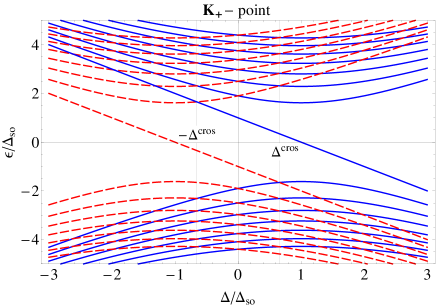
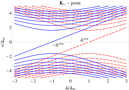
Figure 1: (Color online) Energies of Landau levels in $\Delta_{\text{SO}}$ units at the $\mathbf{K}_{\pm}$ points (upper and lower panels, respectively) as a function of $\Delta/\Delta_{\text{SO}}$ for $\Delta_{R}=0$ and $\hbar\omega=1.62\Delta_{\text{SO}}$. The solid (blue) and dashed (red) curves correspond to $\sigma=\uparrow,\downarrow$, respectively.

The transition from a TI to a BI occurs at the critical value of the gap, $|\Delta|=\Delta_{c}$, where $\Delta_{c}=E_{c}d=\Delta_{\text{SO}}$. Indeed, as one can see in Fig. 1 for $|\Delta|<\Delta_{c}$ in the TI regime the $n=0$ spin up Landau levels at the $\mathbf{K}_{\pm}$ points have a positive energy, while the corresponding spin down levels have a negative energy. In the BI regime for $|\Delta|>\Delta_{c}$ the signs of the energies of the $n=0$ spin up levels at the $\mathbf{K}_{\pm}$ points are opposite. The points of adjacent level (with $n-n^{\prime}=\pm 1$ and $\sigma^{\prime}=-\sigma$) crossing at $\Delta=\pm\Delta^{\mathrm{cros}}$ are marked in Fig. 1 by the vertical lines.

Concluding the overview of the results with zero Rashba term, we note that there are other Dirac materials such as MoS₂ that despite having a different atomic structure are still described by the Hamiltonian (6) with $\Delta_{\text{SO}}\ll|\Delta|$ in the low-energy approximation. Accordingly, the spectrum of Landau levels in MoS₂ Rose2013PRB is the same as considered above.

III.2 Landau levels in the presence of Rashba term

Now we consider the eigenstates $\Psi^{n}_{\xi}$ of the Hamiltonian (13) satisfying $\mathcal{H}_{\xi}\Psi^{n}_{\xi}=\epsilon\Psi^{n}_{\xi}$ for the $R\neq 0$ case Ezawa2012JPSJ . For $n\geq 1$ these eigenstates represent the mixture of four states from three different Landau levels

$$\Psi^{n}_{\xi}=(u_{{\xi}\uparrow}^{n-1}|n-1\rangle,v_{{\xi}\uparrow}^{n}|n\rangle,u_{{\xi}\downarrow}^{n}|n\rangle,v_{{\xi}\downarrow}^{n+1}|n+1\rangle)^{T}$$ (16)

with $|n\rangle=\frac{1}{\sqrt{n!}}(\hat{a}^{\dagger})^{n}|0\rangle$. Then the coefficients $u_{{\xi}s}^{n}$ are the characteristic vectors of the matrix

$$\mathcal{H}_{\xi}^{n}=\xi\begin{pmatrix}\Delta_{\xi\uparrow}&\sqrt{n}\hbar\omega&-i\sqrt{n}R&0\\ \sqrt{n}\hbar\omega&-\Delta_{\xi\uparrow}&0&i\sqrt{n+1}R\\ i\sqrt{n}R&0&\Delta_{\xi\downarrow}&\sqrt{n+1}\hbar\omega\\ 0&-i\sqrt{n+1}R&\sqrt{n+1}\hbar\omega&-\Delta_{\xi\downarrow}\end{pmatrix}.$$ (17)

The corresponding eigenenergies are found from the characteristic quartic equation $\det(\mathcal{H}_{\xi}^{n}-\epsilon\hat{I})=0$ which takes the form

$$\begin{split}&\epsilon^{4}-\left[2(\Delta_{\text{SO}}^{2}+\Delta^{2})+(2n+1)\hbar^{2}\tilde{\omega}^{2}\right]\epsilon^{2}\\ &+\left(\Delta_{\xi\uparrow}^{2}+n\hbar^{2}\tilde{\omega}^{2}\right)\left(\Delta_{\xi\downarrow}^{2}+(n+1)\hbar^{2}\tilde{\omega}^{2}\right)\\ &+2R^{2}\Delta\left[\xi(\epsilon+\Delta_{\text{SO}})-(2n+1)\Delta\right]=0,\end{split}$$ (18)

where

$$\hbar\tilde{\omega}=\sqrt{\hbar^{2}\omega^{2}+R^{2}}$$ (19)

is the Landau scale renormalized by the Rashba term. Writing Eq. (18) we explicitly isolated the last $\sim R^{2}\Delta$ term; its absence would make this equation biquadratic.

For $n=-1$ the eigenstate is

$$\Psi^{-1}_{\xi}=(0,0,0,v_{\xi\downarrow}^{0}|0\rangle)^{T},$$ (20)

with the energy

$$\epsilon_{0\xi\downarrow}=-\xi\Delta_{\xi\downarrow}.$$ (21)

This solution is represented by the dashed (red) straight lines in Fig. 1. Thus for $R\neq 0$ only two out of the four energy levels from (15) with $n=0$ that include only one state from the lowest Landau level $|0\rangle$ remain independent of the strength of the magnetic field.

For $n=0$ the eigenstate represents the mixture of three states from two different Landau levels

$$\Psi^{0}_{\xi}=(0,v_{\xi\uparrow}^{0}|0\rangle,u_{\xi\downarrow}^{0}|0\rangle,v_{\xi\downarrow}^{1}|1\rangle)^{T}.$$ (22)

The corresponding third order characteristic equation has the form

$$\begin{split}&\epsilon^{3}+\xi\Delta_{\xi\uparrow}\epsilon^{2}-(\hbar^{2}\tilde{\omega}^{2}+\Delta_{\xi\downarrow}^{2})\epsilon\\ &-\xi\Delta_{\xi\uparrow}(\hbar^{2}\tilde{\omega}^{2}+\Delta_{\xi\downarrow}^{2})+2\xi\Delta R^{2}=0.\end{split}$$ (23)

In the $R=0$ limit the first root of Eq. (23) is

$$\epsilon_{0\xi\uparrow}=-\xi\Delta_{\xi\uparrow}.$$ (24)

One can see that it corresponds to the other two $n=0$ levels given by Eq. (15) which are shown in Fig. 1 as the solid (blue) straight lines. The other two roots for $R=0$ are

$$\epsilon_{1\xi\downarrow}^{\pm}=\pm\sqrt{\Delta_{\xi\downarrow}^{2}+\hbar^{2}\omega^{2}}$$ (25)

which reproduces two (out of four) of the $n=1$ Landau levels from Eq. (15).

As we already mentioned the description of monolayer low-buckled Dirac materials resembles the formalism developed for a biased bilayer graphene Mucha2009JPCM ; Mucha2009SSC ; Pereira2007PRB ; Zhang2011PRB . The former case is simpler, because the analytically solvable model Hamiltonian (13) contains all relevant parameters. In contrast, to capture the physics of bilayer graphene it is necessary to include the trigonal warping term, presence of which makes the analysis of the Landau level spectra totally numerical.

In spite of a possibility to solve the quartic equation (18) and cubic equation (23) analytically, such general solutions are not particularly useful due to their complexity. Thus we present in Fig. 2 the numerical solutions of Eqs. (18) and (23). The same values of the parameters as in Fig. 1 are taken, but for a better readability of the figure we used the exaggerated value of the Rashba coupling constant, $\Delta_{R}=150\Delta_{\text{SO}}$.

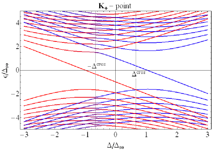
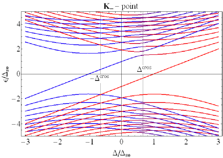
Figure 2: (Color online) Energies of Landau levels in $\Delta_{\text{SO}}$ units at the $\mathbf{K}_{\pm}$ points (upper and lower panels, respectively) as a function of $\Delta/\Delta_{\text{SO}}$ for $\Delta_{R}=150\Delta_{\text{SO}}$ and $\hbar\omega=1.62\Delta_{\text{SO}}$. The color marking corresponds to the not conserving spin quantum number: blue and red correspond to $\sigma=\uparrow,\downarrow$, respectively, and their mixture reflects the superposition of the spins.

Although for $\Delta_{R}\neq 0$ spin is not conserving quantum number, it is instructive to extend the color marking scheme of Fig. 1 and represent the exact spin $|\!\uparrow\,\rangle$ and $|\!\downarrow\,\rangle$ states by the blue and red colors, respectively, and mark the superposition spin state $|\alpha\rangle=a|\!\uparrow\,\rangle+b|\!\downarrow\,\rangle$ by the mixture of the colors in RGB space $\{|b|^{2},0,|a|^{2}\}$. We observe that for $|\Delta|\gg\Delta_{\text{SO}}$ the spin states remain practically pure and their mixing occurs only in the vicinity of the anticrossing points. At these points $a=b=1/2$.

Figure 2 is similar to but not identical with the corresponding figure from the paper of Ezawa Ezawa2012JPSJ , because the continuum model (10) has some sign difference. In particular, we observe that in Fig. 2 for the $\mathbf{K}_{+}$ point the adjacent level ($n-n^{\prime}=\pm 1$ and $\sigma^{\prime}=-\sigma$) anticrossing occurs at $\Delta=-\Delta^{\mathrm{cros}}$, while for the $\mathbf{K}_{-}$ point the adjacent level anticrossing takes place at $\Delta=\Delta^{\mathrm{cros}}$. At first glance, the influence of the Rashba term on the spectrum of the low lying Landau levels turns out to be essential only near the anticrossing points, while outside of these regions the pattern of the Landau levels remains almost unchanged as compared to Fig. 1. A careful analysis shows that the situation is more complicated.

To look closer at the impact of the Rashba term, in Fig. 3 we plotted the dependence of the energy difference $\delta\epsilon=\epsilon_{n\xi}(R\neq 0,\Delta)-\epsilon_{n\xi}(R=0,\Delta)$ on the value of the gap $\Delta$ at the $\mathbf{K}_{-}$ point for four different Landau levels. The long dashed (red) curve is for $n=1$, the dash–dotted (black) curve is for $n=10$, solid (blue) curve is for $n=10^{2}$, and the short dashed (green) is for $n=10^{3}$.

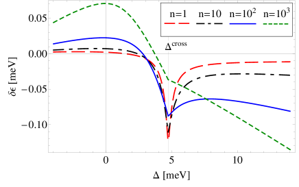
Figure 3: (Color online) The dependence of the energy difference $\delta\epsilon=\epsilon_{n\xi}(R\neq 0,\Delta)-\epsilon_{n\xi}(R=0,\Delta)$ in meV as a function of $\Delta$ in meV for $n=1,10,10^{2},10^{3}$ at the $\mathbf{K}_{-}$ point, $B=\SI{0.2}{T}$, $\Delta_{\text{SO}}=\SI{4.2}{meV}$, and $\Delta_{R}=\SI{21}{meV}$. The Fermi velocity $v_{F}=5.5\times 10^{5}\mbox{m/s}$.

We observe that for small $n=1-10$ the Rashba term is indeed important only near the anticrossing point, $\Delta=-\xi\Delta^{\mathrm{cros}}$. Moreover, its impact on the spectrum at the point $\Delta=-\xi\Delta^{\mathrm{cros}}$ is stronger for smaller $n$. On the other hand, for large $n\gtrsim 100$ the Rashba term becomes more important for $|\Delta|\gtrsim\Delta^{\mathrm{cros}}$.

Now we proceed to the discussion of the cases where the analytical work can provide more insight to the role of the Rashba term.

III.3 Analytical treatment of the Rashba term

The analytical consideration of the Rashba term may be useful in the following cases.
(i) One can obtain a simple generalization of the spectrum (15) which would allow one to consider the influence of the Rashba SO coupling on quantum magnetic oscillations as done below in Sec. IV.
(ii) One can derive a simple expression for the correction to the unperturbed spectrum (15) when the values of the parameters $\Delta,B$ are specially adjusted, e.g. in the vicinity of the anticrossing point.

III.3.1 The $\Delta=0$ case

As we already mentioned, the induced by the on-site potential difference between sublattices gap $\Delta$ can be tuned by adjusting the electric field $E_{z}$. Thus it is possible to realize the $\Delta=0$ case. Then the last term of Eqs. (18) and (23) becomes zero making these equations biquadratic. Then the energies of the Landau levels are still given by Eq. (15), but the Landau scale (14) has to be replaced by the renormalized scale $\hbar\tilde{\omega}$ defined in Eq. (19).

It is convenient to express the renormalized Landau scale $\hbar\tilde{\omega}=\sqrt{2}\hbar{\tilde{v}}_{F}/l_{B}$ in terms of the renormalized Fermi velocity ${\tilde{v}}_{F}^{2}=v_{F}^{2}+v_{R}^{2}$, where we introduced the velocity $v_{R}=\Delta_{R}a/\hbar$ associated with the Rashba coupling. Using the characteristic values of the lattice constant $a=3.86\mathring{A}$ and Fermi velocity $v_{F}=5.5\times 10^{5}\,\mbox{m/s}$ for silicene, and assuming that the Rashba term is $\Delta_{R}=\kappa[\mbox{meV}]$, one can estimate the ratio $v_{R}/v_{F}=\kappa 1.1\times 10^{-3}$. This indicates that the impact of the Rashba term is rather small in the considered case unless $\Delta_{R}$ is really large.

III.3.2 Landau levels in the quasiclassical regime

In the quasiclassical limit, $n\gg 1$ one can neglect the difference between the factors $\sqrt{n}$ and $\sqrt{n+1}\approx\sqrt{n}$ in the matrix Hamiltonian (17). Then the corresponding characteristic equation acquires the form

$$\begin{split}&\epsilon^{4}-2\left(\Delta^{2}+\Delta_{\text{SO}}^{2}+n\hbar^{2}\tilde{\omega}^{2}\right)\epsilon^{2}+\\ &\left(\Delta_{\xi\uparrow}^{2}+n\hbar^{2}\tilde{\omega}^{2}\right)\left(\Delta_{\xi\downarrow}^{2}+n\hbar^{2}\tilde{\omega}^{2}\right)-4n\Delta^{2}R^{2}=0,\end{split}$$ (26)

where we used the renormalized Landau scale (19) and separated the last $\sim R^{2}$ term. One can notice that Eq. (26) follows from the general equation (18) if in addition to $n\gg 1$ one assumes that $|\epsilon|,|\Delta_{\text{SO}}|\ll n|\Delta|$. It is easy to solve the biquadratic equation (26) to obtain the large $n$ spectrum

$$\begin{split}&\epsilon_{n\xi\sigma}^{\pm}=\\ &\pm\sqrt{\Delta^{2}+\Delta_{\text{SO}}^{2}+n\hbar^{2}\tilde{\omega}^{2}-2\xi s_{\sigma}\Delta\sqrt{\Delta_{\text{SO}}^{2}+nR^{2}}}.\end{split}$$ (27)

Here the factor $\xi s_{\sigma}$ guarantees that for $R=0$ the spectrum (27) agrees with Eq. (15) for $n>0$.

The spectrum (27) also follows from the Lifshitz-Onsager quantization condition for the cross-sectional area of the orbit in momentum space,

$$S(\epsilon)=(n+\gamma)2\pi\hbar\frac{eB}{c}.$$ (28)

One can check this rewriting the area of the orbit $S(\epsilon)=\pi\hbar^{2}k^{2}$ via the momentum $\hbar\mathbf{k}$ expressed from the inverse zero field dispersion relationship (11). Then assuming that the phase $\gamma=0$, as it should be in the case of the massive Dirac fermions Sharapov2004PRB (see also Refs. Carmier2008PRB ; Fuchs2010EPJB , where the role of the semiclassical “Berry-like” phase is studied), and solving Eq. (28) with respect to the energy $\epsilon$ one reproduces the large $n$ spectrum (27).

III.3.3 Energies of the Landau levels near the level anticrossing points

The points of level crossing are shown in Fig. 1 computed for the $\Delta_{R}=0$ case. They are determined by the condition $\epsilon_{n\xi\sigma}=\epsilon_{n^{\prime}\xi\sigma^{\prime}}$, where the energy $\epsilon_{n\xi\sigma}$ is given by Eq. (15). Then the level crossing condition acquires the form Ezawa2012JPSJ

$$(n-n^{\prime})\hbar^{2}\omega^{2}=2\xi(s_{\sigma}-s_{\sigma^{\prime}})\Delta\Delta_{\text{SO}}.$$ (29)

Accordingly we obtain that the branches with the opposite spin, $s_{\sigma}^{\prime}=-s_{\sigma}$, cross when the value of the gap is

$$\Delta=\pm(n-n^{\prime})\Delta^{\mathrm{cros}},\qquad\Delta^{\mathrm{cros}}=\frac{\hbar^{2}\omega^{2}}{4\Delta_{\text{SO}}}.$$ (30)

Comparing Figs. 1 and 2 we saw that for $R\neq 0$ the anticrossing occurs only at the points $\Delta=-\xi\Delta^{\mathrm{cros}}$.

As shown above the energy $\epsilon_{0\xi\downarrow}$ of the lowest Landau level given by Eq. (21) does not depend on $B$ both for $R=0$ and $R\neq 0$. The energies of the other low lying levels are determined by Eq. (23). For $R=0$ its solutions are given by Eqs. (24) and (25). As we already saw, the first root is shown in Fig. 1 as the solid (blue) straight lines and the other two roots are given by the dashed (red) parabolas with the lowest absolute value of the energy. It is easy to check that at the energies $E_{n\xi\sigma}^{\pm}\equiv\epsilon_{n\xi\sigma}^{\pm}(\Delta=-\xi\Delta^{\mathrm{cros}})$ there is indeed level crossing, viz.

$$E_{0\xi\uparrow}=E^{+}_{1\xi\downarrow}=\Delta_{\text{SO}}+\frac{\hbar^{2}\omega^{2}}{4\Delta_{\text{SO}}}.$$ (31)

To estimate how the presence of Rashba term, $R\neq 0$ changes these energies when level crossing switches to anticrossing, one seeks a solution of Eq. (23) in the following form, $\epsilon(R)=\epsilon(R=0)+\delta\epsilon$. The corresponding equation for an energy perturbation $\delta\epsilon$ is

$$\delta\epsilon^{3}+2\Delta_{\xi\uparrow}\delta\epsilon^{2}-(\hbar^{2}\omega^{2}+4\xi\Delta\Delta_{\text{SO}}+R^{2})\delta\epsilon+2\xi\Delta R^{2}=0.$$ (32)

For $\delta E=\delta\epsilon(\Delta=-\xi\Delta^{\mathrm{cros}})$ Eq. (32) acquires the form

$$2\Delta_{\text{SO}}\delta E^{3}+(\hbar^{2}\omega^{2}+4\Delta_{\text{SO}}^{2})\delta E^{2}-2\xi\Delta_{\text{SO}}R^{2}\delta E-\hbar^{2}\omega^{2}R^{2}=0.$$ (33)

We found that the relevant solution of the last equation can be approximated by the following linear in $R$ expression

$$\delta E\approx\pm\frac{\hbar\omega R}{\sqrt{\hbar^{2}\omega^{2}+4\Delta_{\text{SO}}^{2}}}$$ (34)

that describes the energy shift of the crossing levels that for $R=0$ had the energy (31). Taking into account that the energy gap between the anticrossed levels corresponds to the doubled level shift $\delta E$, one can check that for $\hbar\omega\gg\Delta_{\text{SO}}$ Eq. (34) reduces to Ezawa’s result Ezawa2012JPSJ

$$2\delta E\approx 2R=2\sqrt{2}\frac{a}{l_{B}}\Delta_{R}.$$ (35)

Now we pass to the higher Landau levels with the energies determined by Eq. (18). For $R=0$ its solutions are given by Eq. (15). Accordingly, we find that at the level anticrossing point, $E_{n\xi\sigma}^{\pm}=\epsilon_{n\xi\sigma}^{\pm}(\Delta=-\xi\Delta^{\mathrm{cros}})$ the energy is

$$E_{n\xi\sigma}^{\pm}=\pm\sqrt{\Delta_{\text{SO}}^{2}+\frac{1}{2}(2n+s_{\sigma})\hbar^{2}\omega^{2}+\frac{\hbar^{4}\omega^{4}}{16\Delta_{\text{SO}}^{2}}}.$$ (36)

One can see that for the adjacent levels $E_{n\xi\uparrow}^{\pm}=E_{(n+1)\xi\downarrow}^{\pm}$, so that for $n=0$ the positive branch of the spectrum reduces to Eq. (31). As in the previous case, we seek for a solution of the equation (18) at the anticrossing point, $\Delta=-\xi\Delta^{\mathrm{cros}}$, in the form $\epsilon(R)=\epsilon(R=0)+\delta\epsilon$ with the perturbation $\delta\epsilon$ caused by a finite $R$. Neglecting $\delta\epsilon^{4}$ term, we found its approximate solution:

$$\begin{split}&\delta E\approx\pm\frac{\hbar\omega R}{2\sqrt{2}\Delta_{\text{SO}}E_{n\xi\sigma}^{+}}\\ &\times\sqrt{\Delta_{\text{SO}}\left(\Delta_{\text{SO}}+E_{n\xi\sigma}^{+}\right)+\frac{1}{2}(2n+s_{\sigma})\frac{\hbar^{2}\omega^{2}}{2}}.\end{split}$$ (37)

This expression represents one of the main results of the present work. Taking $n=0$ and $\sigma=\uparrow$ in Eq. (37) one can verify that it reduces to the derived above Eq. (34).

We plot in Figs. 4 and 5 the exact result based on the numerical solution of Eq. (18) and the approximate expression (37) to investigate the range of its validity. Figure 4 shows the dependence of the relative energy shift $\delta E/E_{n\xi\sigma}^{+}=[\epsilon_{n\xi}(R\neq 0,\Delta=-\xi\Delta^{\mathrm{cros}})-\epsilon_{n\xi}(R=0,\Delta=-\xi\Delta^{\mathrm{cros}})]/E_{n\xi\sigma}^{+}$ at $\mathbf{K}_{-}$ point as a function of magnetic field $B$ for a fixed value of $\Delta_{R}$ and four different values of $n=0,1,10,100$. The values $\Delta_{\text{SO}}=10\,\text{meV}$ and $\Delta_{R}=50\,\text{meV }$ are taken. The thick lines are plotted using the energy difference $\delta E=\epsilon_{n\xi}(R\neq 0,\Delta=-\xi\Delta^{\mathrm{cros}})-\epsilon_{n\xi}(R=0,\Delta=-\xi\Delta^{\mathrm{cros}})$ which is computed using the numerical solution of the general Eq. (18) and the thin lines are calculated using the approximate Eq. (37).

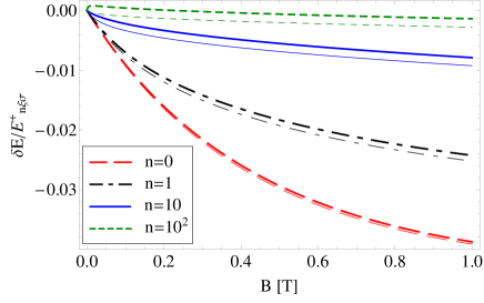
Figure 4: (Color online) The dependence of the relative energy shift $\delta E/E_{n\xi\sigma}^{+}$ at $\mathbf{K}_{-}$ point as a function of magnetic field $B$ for $\Delta_{\text{SO}}=10\,\text{meV}$ and $\Delta_{R}=50\,\text{meV }$. The long-dashed (red) line is for $n=0$, $n=1$ -— the dash-dotted (black) line, $n=10$ – the solid (blue) line, and $n=100$ – the short-dashed (green) line. All thick lines are plotted using the energy difference $\delta E=\epsilon_{n\xi}(R\neq 0,\Delta=-\xi\Delta^{\mathrm{cros}})-\epsilon_{n\xi}(R=0,\Delta=-\xi\Delta^{\mathrm{cros}})$ which is computed using the numerical solution of the general Eq. (18) and the thin lines are calculated using the approximate Eq. (37).

We observe that the expression for $\delta E$ provides rather good approximation for the energy shift at the anticrossing point for all values of $n$ and even for a large value of $\Delta_{R}$.

In Fig. 5 we plotted the dependence of the relative energy shift $\delta E/E_{n\xi\sigma}^{+}$ at $\mathbf{K}_{-}$ point as a function of magnetic field $B$ for three values of $\Delta_{R}=1\,\mbox{meV}$, $\Delta_{R}=5\,\mbox{meV}$, and $\Delta_{R}=10\,\mbox{meV}$ for fixed $n=50$ and $\Delta_{\text{SO}}=10\,\text{meV}$.

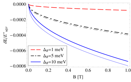
Figure 5: (Color online) The dependence of the relative energy shift $\delta E/E_{n\xi\sigma}^{+}$ at $K_{-}$ point as a function of magnetic field $B$ for $\Delta_{\text{SO}}=10\,\text{meV}$ and $n=50$. The dashed (red) line is for $\Delta_{R}=1\,\mbox{meV}$ , $\Delta_{R}=5\,\mbox{meV}$ – the dash-dotted (black) line, and $\Delta_{R}=10\,\mbox{meV}$ – solid (blue) line. All thick lines are plotted using the energy difference $\delta E=\epsilon_{n\xi}(R\neq 0,\Delta=-\xi\Delta^{\mathrm{cros}})-\epsilon_{n\xi}(R=0,\Delta=-\xi\Delta^{\mathrm{cros}})$ which is computed using the numerical solution of the general Eq. (18) and the thin lines are calculated using the approximate Eq. (37).

We also observe that for a small value of $\Delta_{R}$ the approximated expression practically coincides with the exact one. As $\Delta_{R}$ increases, the approximate result deviates from the exact one. This is not surprising, because the expression (37) was obtained using a linear in $R$ approximation.

IV The density of states

In the absence of scattering from impurities the density of states (DOS) is expressed via the energies of the Landau levels $\epsilon_{n\xi\sigma}^{\lambda}$ as follows:

$$D_{0}(\varepsilon)=\frac{eB}{2\pi\hbar c}\sum_{\begin{subarray}{c}\sigma=\downarrow,\uparrow\\ \xi=\pm\end{subarray}}\sum_{\lambda=\pm}\sum_{n=0}^{\infty}\delta(\varepsilon-\epsilon_{n\xi\sigma}^{\lambda}).$$ (38)

The broadening of Landau levels due to the scattering from impurities can be taken into account 1984ShonbergBook by convolution of the DOS $D_{0}(\omega)$ with zero level broadening with the distribution function $P_{\Gamma}(\omega)$, viz.

$$D(\varepsilon)=\int\limits_{-\infty}^{\infty}d\omega P_{\Gamma}(\omega-\varepsilon)D_{0}(\omega),\qquad\int\limits_{-\infty}^{\infty}d\omega P_{\Gamma}(\omega)=1.$$ (39)

The simplest model for the level broadening (39) is the Lorentz distribution, $P_{\Gamma}(\omega)=\Gamma/\left[\pi(\omega^{2}+\Gamma^{2})\right]$ with the impurity scattering rate $\Gamma$.

In its turn the knowledge of zero temperature DOS is completely sufficient to write down the finite temperature thermodynamic potential and other thermodynamic quantities. Moreover, the DOS can be experimentally found by measuring the quantum capacitance $C$ Ponomarenko2010PRL ; Yu2013PNAS , which is proportional to the thermally smeared DOS and is given by

$$C(\mu)=e^{2}\int\limits_{-\infty}^{\infty}d\varepsilon D(\varepsilon)\left(-n_{F}^{\prime}(\varepsilon)\right),$$ (40)

where $n_{F}(\varepsilon)=1/[\exp(\varepsilon-\mu)/T+1]$ is the Fermi distribution.

IV.1 The DOS in the absence of Rashba term

As was discussed in the Introduction, the electron subsystem in the considered Dirac materials for $\Delta_{R}=0$ turns out to be equivalent to two independent layers of the gapped monolayer graphene with the gaps $\Delta\pm\Delta_{\text{SO}}$. Indeed, the $R=0$ spectrum (15) for a fixed value of the spin $\sigma$ reduces to the well-known spectrum of the gapped graphene Haldane1988PRL (see also Appendix D of Ref. Gusynin2006PRB ). Thus using the results of Ref. Sharapov2004PRB one can straightforwardly write the final expressions for the DOS.

In the absence of scattering from impurities using the Poisson summation formula one can derive from Eq. (38) the following expression:

$$\begin{split}&D_{0}(\varepsilon)=\frac{1}{2\pi v_{F}^{2}\hbar^{2}}\sum_{\sigma=\downarrow,\uparrow}\mbox{sgn}(\varepsilon)\frac{d}{d\varepsilon}\Bigg{(}\theta(\varepsilon^{2}-\Delta_{+\sigma}^{2})\times\\ &\left.\left[\varepsilon^{2}-\Delta_{+\sigma}^{2}+\hbar^{2}\omega^{2}\sum_{k=1}^{\infty}\frac{1}{\pi k}\sin\left(\frac{2\pi k(\varepsilon^{2}-\Delta_{+\sigma}^{2})}{\hbar^{2}\omega^{2}}\right)\right]\right).\end{split}$$ (41)

The DOS (41) contains oscillations with the two frequencies $2\pi k(\varepsilon^{2}-\Delta_{+\downarrow}^{2})/(\hbar^{2}\omega^{2})$ and $2\pi k(\varepsilon^{2}-\Delta_{+\uparrow}^{2})/(\hbar^{2}\omega^{2})$. The oscillatory part of the DOS can be written in the form of the beats

$$\begin{split}&D_{0}^{\mathrm{osc}}(\varepsilon)=\frac{2}{\pi^{2}l_{B}^{2}}\mbox{sgn}(\varepsilon)\\ &\times\left[\frac{d}{d\varepsilon}\sum_{k=1}^{\infty}\frac{1}{k}\sin\left(\frac{2\pi kF_{o}}{B}\right)\cos\left(\frac{2\pi kF_{b}}{B}\right)\right],\end{split}$$ (42)

where

$$F_{o}=\frac{\varepsilon^{2}-\Delta_{\text{SO}}^{2}-\Delta^{2}}{2v_{F}^{2}\hbar e/c}$$ (43)

is the frequency (for $k=1$) of oscillations in $1/B$ and

$$F_{b}=\frac{\Delta_{\text{SO}}\Delta}{v_{F}^{2}\hbar e/c}$$ (44)

is the frequency (for $k=1$) of beats. In deriving Eq. (42) we assumed that $|\varepsilon|>|\Delta\pm\Delta_{\text{SO}}|$. For $\varepsilon^{2}\gg|\Delta_{\text{SO}}\Delta|$ the frequency of beats $F_{b}\ll F_{o}$. Notice that in the absence of the Rashba interaction the frequency $F_{b}$ depends solely on the SO gap $\Delta_{\text{SO}}$ and is tunable by the applied electric field gap $\Delta$.

In the case of the distribution function $P_{\Gamma}(\omega)$ given by the Lorentzian distribution, the sum over Landau levels can be expressed in the closed form Sharapov2004PRB in terms of the digamma function $\psi$. Accordingly, the DOS of silicene represents the sum of the two terms

$$\begin{split}&D(\varepsilon)=\frac{1}{\pi^{2}v_{F}^{2}\hbar^{2}}\left\{2\Gamma\ln\left(\frac{\Lambda^{2}}{2\hbar v_{F}^{2}eB/c}\right)-\mbox{Im}\left[(\varepsilon+i\Gamma)\times\right.\right.\\ &\left.\left.\sum_{\sigma=\downarrow,\uparrow}\left(\psi\left(\frac{\Delta_{+\sigma}^{2}-(\varepsilon+i\Gamma)^{2})}{2\hbar v_{F}^{2}eB/c}\right)+\frac{\hbar v_{F}^{2}eB/c}{\Delta_{+\sigma}^{2}-(\varepsilon+i\Gamma)^{2})}\right)\right]\right\},\end{split}$$ (45)

where $\Lambda$ is the energy cutoff associated with the bandwidth. Its presence in the nonoscillatory part of the DOS is related to the Lorentzian shape of the level broadening.

Equation (45) turns out to be convenient for numerical modeling of the DOS when the width of all Landau levels is the same. In the case when each level has a different width Eq. (38) acquires the form

$$D_{0}(\varepsilon)=\frac{1}{2\pi^{2}l_{B}^{2}}\sum_{\begin{subarray}{c}\sigma=\downarrow,\uparrow\\ \xi=\pm\end{subarray}}\sum_{\lambda=\pm}\sum_{n=0}^{\infty}\frac{\Gamma_{n\xi\sigma}^{\lambda}}{(\varepsilon-\epsilon_{n\xi\sigma}^{\lambda})^{2}+(\Gamma_{n\xi\sigma}^{\lambda})^{2}}.$$ (46)

Since the level width $\Gamma_{n\xi\sigma}^{\lambda}$ is in general unknown, it is impossible to use the Poisson formula or to sum over Landau levels as done above. It is possible instead to consider analytically the thermal smearing of the DOS which is present in the capacitance (40). The final results obtained in Ref. Gusynin2014FNT, can be rewritten as follows

$$C(\mu)=\frac{e^{2}}{2\pi^{2}l_{B}^{2}}\sum_{\begin{subarray}{c}\sigma=\downarrow,\uparrow\\ \xi=\pm\end{subarray}}\sum_{\lambda=\pm}\sum_{n=0}^{\infty}I(\mu-\epsilon_{n\xi\sigma}^{\lambda},\Gamma_{n\xi\sigma}^{\lambda}),$$ (47)

where

$$I(\epsilon,\Gamma)=\frac{1}{2\pi T}\mbox{Re}\psi^{\prime}\left(\frac{1}{2}+\frac{\Gamma-i\epsilon}{2\pi T}\right)$$ (48)

is expressed in terms of the derivative of the digamma function $\psi$. The capacitance (47) already includes both thermal and impurity averages and only the sum over Landau levels is left for the numerical calculation. Equation (47) is in fact valid not only for $R=0$. In the $R\neq 0$ case instead of the energies $\epsilon_{n\xi\sigma}^{\lambda}$ given by Eq. (15) one should use the energies of the corresponding Landua levels found in Sec. III.2.

IV.2 The DOS in the presence of Rashba term

The expression (42) presented above can be generalized for the case of $\Delta_{R}\neq 0$. The analytical expression (27) valid in the large $n$ limit allows one to evaluate the sum over Landau levels. First Eq. (38) can be rewritten as follows:

$$D_{0}(\varepsilon)=\frac{eB}{\pi\hbar c}\mbox{sgn}\,\varepsilon\frac{d}{d\varepsilon}\sum_{\sigma=\uparrow,\downarrow}\sum_{n=0}^{\infty}\theta(\epsilon^{2}-(\epsilon_{n+\sigma}^{+})^{2}),$$ (49)

where the summation over $\lambda,\xi=\pm$ is done. Then using the Poisson summation formula

$$\begin{split}&\frac{1}{2}F(0)+\sum\limits_{n=1}^{\infty}F(n)\\ &=\int\limits_{0}^{\infty}F(x)dx+2{\rm Re}\sum\limits_{k=1}^{\infty}\int\limits_{0}^{\infty}F(x)e^{2\pi ikx}dx,\end{split}$$ (50)

we find that the oscillatory part of the DOS can still be written in the form of Eq. (42). The frequency of oscillations

$$F_{o}\approx\frac{\varepsilon^{2}-\Delta_{\text{SO}}^{2}-\Delta^{2}+2(v_{R}^{2}/v_{F}^{2})\Delta^{2}}{2v_{F}^{2}\hbar e/c}$$ (51)

is now shifted with respect to its $\Delta_{R}=0$ value given by Eq. (43). Since the ratio $v_{R}/v_{F}$ is small (see Sec. III.3.1) and the new term can be absorbed by renormalizing the value of $\Delta$ one can conclude that this shift of the oscillation frequency cannot be used to determine the Rashba term. The situation with the frequency of beats $F_{b}$ seems to be more promising. Indeed, Eq. (44) acquires the form

$$F_{b}=\frac{\Delta_{\text{SO}}\Delta}{v_{F}^{2}\hbar e/c}\left(1+\frac{1}{2}\frac{v_{R}^{2}}{v_{F}^{2}}\frac{\varepsilon^{2}-\Delta^{2}-\Delta_{\text{SO}}^{2}}{\Delta_{\text{SO}}^{2}}\right).$$ (52)

We observe that in the last term in the brackets of Eq. (52) the smallness of the ratio $v_{R}^{2}/v_{F}^{2}\sim\kappa^{2}\times 10^{-6}$ can be compensated by the large value of the ratio $\varepsilon^{2}/\Delta_{\text{SO}}^{2}$. Even more important is that due this term the frequency $F_{b}$ is now dependent on the position of the Fermi level, $\varepsilon=\mu$, and, accordingly, on the carrier concentration.

V Conclusion

We studied how the pattern of Landau levels in the low-buckled Dirac materials is modified by the intrinsic Rashba SO coupling between NNN. In particular, we found the approximate analytical expressions (34) and (37) for the energy shift caused by the Rashba term in the vicinity of the level anticrossing points. The impact of the Rashba interaction is maximal in this regime.

We also derived the analytical expression (27) for energies of the Landau levels in the large $n$ limit. Its relatively simple form allowed us to derive the analytical expression describing quantum magnetic oscillations of the DOS. A specific feature of the oscillations is the presence of the beats caused by crossing of the Fermi level by the Landau levels from the two different branches of the quasiparticle excitations. These beats resemble the oscillatory effects observed in the usual 2D electron gas with parabolic dispersion and Rashba interaction Bychkov1984JPCS . When the Rashba interaction is absent, the frequency of beats $F_{b}$ is given by Eq. (43). It is proportional to the product $\Delta_{\text{SO}}\Delta$, where the sublattice asymmetry gap $\Delta$ can be controlled by the applied electric field $E_{z}$. In the presence of the intrinsic Rashba interaction the frequency $F_{b}$ shifts (51) and becomes dependent both on the gap $\Delta$ and carrier concentration. This peculiarity can be helpful for the experimental determination of the value of the Rashba coupling constant.

Our results are applicable in the analysis of a number of experiments which probe transport and thermodynamic properties of the low-buckled Dirac materials, including cyclotron resonance, tunneling spectroscopy, capacitance measurements, charge compressibility, and magnetization. Concluding we also note that these results may be applicable for a wider range of materials, e.g., for a bilayer TI Zhang20013PRL .

- (1) B. Lalmi, H. Oughaddou, H. Enriquez, A. Kara, S. Vizzini, B. Ealet, and B. Aufray, Appl. Phys. Lett. 97, 223109 (2010).
- (2) P. De Padova, C. Quaresima, C. Ottaviani, P. M. Sheverdyaeva, P. Moras, C. Carbone, D. Topwal, B. Olivieri, A. Kara, H. Oughaddou, B. Aufray, and G. Le Lay, Appl. Phys. Lett. 96, 261905 (2010).
- (3) P. De Padova, C. Quaresima, B. Olivieri, P. Perfetti, and G. Le Lay, Appl. Phys. Lett. 98, 081909 (2011).
- (4) P. Vogt, P. De Padova, C. Quaresima, J. Avila, E. Frantzeskakis, M. C. Asensio, A. Resta, B. Ealet, and G. Le Lay, Phys. Rev. Lett. 108, 155501 (2012).
- (5) C.-L. Lin, R. Arafune, K. Kawahara, N. Tsukahara, E. Minamitani, Y. Kim, N. Takagi, and M. Kawai, Appl. Phys. Express 5, 045802 (2012).
- (6) A. Fleurence, R. Friedlein, T. Ozaki, H. Kawai, Y. Wang, and Y. Yamada-Takamura, Phys. Rev. Lett. 108, 245501 (2012).
- (7) L. Chen, C.-C. Liu, B. Feng, X. He, P. Cheng, Z. Ding, S. Meng, Y. Yao, and K. Wu, Phys. Rev. Lett. 109, 056804 (2012).
- (8) Z. Majzik, M.R. Tchalala, M. Svec, P. Hapala, H. Enriquez, A. Kara, A.J. Mayne, G. Dujardin, P. Jelíınek, and H. Oughaddou, J. Phys.: Cond. Mat. 25, 225301 (2013).
- (9) S. Cahangirov, M. Topsakal, E. Aktürk, H. Şahin, and S. Ciraci, Phys. Rev. Lett. 102, 236804 (2009).
- (10) N. D. Drummond, V. Zólyomi, and V. I. Fal’ko, Phys. Rev. B 85, 075423 (2012).
- (11) C.-C. Liu, W. Feng, and Y. Yao, Phys. Rev. Lett. 107, 076802 (2011).
- (12) C.-C. Liu, H. Jiang, and Y. Yao, Phys. Rev. B 84, 195430 (2011).
- (13) W.-F. Tsai, C.-Y. Huang, T.-R. Chang, H. Lin, H.-T. Jeng, and A. Bansil, Nature Commun. 4, 1500 (2013).
- (14) Y. Xu, B. Yan, H.-J. Zhang, J. Wang,G. Xu, P. Tang, W. Duan, and S.-C. Zhang, Phys. Rev. Lett. 111, 136804 (2013).
- (15) M. Ezawa, New J. Phys. 14, 033003 (2012).
- (16) M. Ezawa, J. Phys. Soc. Jpn. 81, 064705 (2012).
- (17) C.J. Tabert and E.J. Nicol, Phys. Rev. Lett. 110, 197402 (2013).
- (18) C.J. Tabert and E.J. Nicol, Phys. Rev. B 88, 085434 (2013).
- (19) A. Dyrdał and J. Barnaś, Phys. Status Solidi (RRL) 6, 340 (2012).
- (20) L. Stille, C. J. Tabert, and E. J. Nicol, Phys. Rev. B 86, 195405 (2012).
- (21) L. Matthes, P. Gori, O. Pulci, and F. Bechstedt, Phys. Rev. B 87, 035438 (2013).
- (22) C.J. Tabert and E.J. Nicol, Phys. Rev. B 87, 235426 (2013).
- (23) V.P. Gusynin, S.G. Sharapov and J.P. Carbotte, Phys. Rev. Lett. 96, 256802 (2006); Phys. Rev. Lett. 98, 157402 (2007); J. Phys.: Cond. Matt. 19, 026222 (2007).
- (24) M. Mucha-Kruczyński, D.S.L. Abergel, E. McCann, and V.I. Fal’ko, Solid State Comm. 149, 1111 (2009).
- (25) M Mucha-Kruczyński, E. McCann, and V.I. Fal’ko, J. Phys.: Cond. Matt. 21, 344206 (2009).
- (26) J.M. Pereira Jr., F.M. Peeters, and P. Vasilopoulos, Phys. Rev. B 76, 115419 (2007).
- (27) L.M. Zhang, M.M. Fogler, and D.P. Arovas, Phys. Rev. B 84, 075451 (2011).
- (28) M. Hohenadler and F.F. Assaad, J. Phys. Cond. Matt. 25, 143201 (2013).
- (29) C. L. Kane and E. J. Mele, Phys. Rev. Lett. 95, 146802; ibid. 95, 226801 (2005).
- (30) A. Varykhalov, J. Sánchez-Barriga, A.M. Shikin, C. Biswas, E. Vescovo, A. Rybkin, D. Marchenko, and O. Rader, Phys. Rev. Lett. 101, 157601 (2008).
- (31) E.I. Rashba, Phys. Rev. B 79, 161409(R) (2009).
- (32) A. De Martino, A. Hütten, and R. Egger, Phys. Rev. B 84, 155420 (2011).
- (33) M. Ezawa, Phys. Rev. Lett. 109, 055502 (2012).
- (34) V.P. Gusynin, S.G. Sharapov, and J.P. Carbotte, Int. J. Mod. Phys. B 21, 4611 (2007).
- (35) G.W. Semenoff, Phys. Rev. Lett. 53, 2449 (1984).
- (36) F.D.M. Haldane, Phys. Rev. Lett. 61, 2015 (1988).
- (37) F. Rose, M.O. Goerbig, F. Piéchon, Phys. Rev. B 88, 125438 (2013).
- (38) S.G. Sharapov, V.P. Gusynin, and H. Beck, Phys. Rev. B 69, 075104 (2004).
- (39) P. Carmier and D. Ullmo, Phys. Rev. B 77, 245413 (2008).
- (40) J.N. Fuchs, F. Piéchon, M.O. Goerbig, and G. Montambaux, Eur. Phys. J. B 77, 351 (2010).
- (41) D. Shoenberg, Magnetic Oscillations in Metals, Cambridge University Press, 1984.
- (42) L.A. Ponomarenko, R. Yang, R.V. Gorbachev, P. Blake, A.S. Mayorov, K.S. Novoselov, M.I. Katsnelson, and A.K. Geim, Phys. Rev. Lett. 105, 136801 (2010).
- (43) G.L. Yu, R. Jalil, B. Belle, A.S. Mayorov, P. Blake, F. Schedin, S.V. Morozov, L.A. Ponomarenko, F. Chiappini, S. Wiedmann, U. Zeitler, M.I. Katsnelson, A.K. Geim, K.S. Novoselov, and D.C. Elias, Proc. Natl. Natl Acad. Sci. USA 110, 3281 (2013).
- (44) V.P. Gusynin and S.G. Sharapov, Phys. Rev. B 73, 245411 (2006).
- (45) V.P. Gusynin, V.M. Loktev, I.A. Luk’yanchuk, S.G. Sharapov, and A.A. Varlamov, Fiz. Nizk. Temp. 40, 355 (2014) Engl. trans.: Low Temp. Phys. 40, 270 (2014).
- (46) Yu.A. Bychkov and E.I. Rashba, J. Phys. C Sol. St. Phys. 17, 6039 (1984).
- (47) Fan Zhang, C.L. Kane, and E.J. Mele, Phys. Rev. Lett. 110, 046404 (2013).