Comparison of multi-fluid moment models with Particle-in-Cell simulations of collisionless magnetic reconnection

Abstract

We introduce an extensible multi-fluid moment model in the context of collisionless magnetic reconnection. This model evolves full Maxwell equations, and simultaneously moments of the Vlasov-Maxwell equation for each species in the plasma. Effects like electron inertia and pressure gradient are self-consistently embedded in the resulting multi-fluid moment equations, without the need to explicitly solving a generalized Ohms’s law. Two limits of the multi-fluid moment model are discussed, namely, the five-moment limit that evolves a scalar pressures for each species, and the ten-moment limit that evolves the full anisotropic, non-gyrotropic pressure tensor for each species. We first demonstrate, analytically and numerically, that the five-moment model reduces to the widely used Hall Magnetohydrodynamics (Hall MHD) model under the assumptions of vanishing electron inertia, infinite speed of light, and quasi-neutrality. Then, we compare ten-moment and fully kinetic Particle-In-Cell (PIC) simulations of a large scale Harris sheet reconnection problem, where the ten-moment equations are closed with a local linear collisionless approximation for the heat flux. The ten-moment simulation gives reasonable agreement with the PIC results regarding the structures and magnitudes of the electron flows, the polarities and magnitudes of elements of the electron pressure tensor, and the decomposition of the generalized Ohm’s law. Possible ways to improve the simple local closure towards a nonlocal fully three-dimensional closure are also discussed.

I Introduction

Magnetic reconnection is the process by which magnetic field line topology changes. It is often accompanied by fast, explosive release of magnetic energy and restructuring of macroscopic quantities of the plasma, such as flows and thermal energy. Reconnection is widely thought to play a critical role in many physical phenomena in laboratory, solar, terrestrial, and astrophysical plasmasYamada, Kulsrud, and Ji (2010); Zweibel and Yamada (2009).

A key constraint in ideal magnetohydrodynamics (MHD) is the frozen-flux constraint $\mathbf{E}+\mathbf{u}\times\mathbf{B}=0$, or, equivalently $E_{\parallel}=0$. With this, field line topology cannot change, and hence reconnection cannot occur. Hence, one must look beyond the ideal MHD model to study reconnection, in particular the generalized Ohm’s law

$$\mathbf{E}+ \mathbf{u}\times\mathbf{B}=\eta\mathbf{J}+\frac{\mathbf{J}\times\mathbf{B}}{n\left|e\right|}-\frac{\nabla\cdot\mathbf{P}_{e}}{n\left|e\right|}$$

$$+\frac{m_{e}}{n\left|e\right|^{2}}\left[\frac{\partial\mathbf{J}}{\partial t}+\nabla\cdot\left(\mathbf{u}\mathbf{J}+\mathbf{J}\mathbf{u}-\frac{\mathbf{JJ}}{n\left|e\right|}\right)\right].$$ (1)

Here, $\eta\mathbf{J}$ is the resistive dissipation term, $\mathbf{J}\times\mathbf{B}/n\left|e\right|$ is the Hall term (which by itself does not change field line topology), $\nabla\cdot\mathbf{P}_{e}/n\left|e\right|$ is electron pressure gradient term, and the last term is proportional to electron inertia. Historically, SweetSweet (1958) and ParkerParker (1957) proposed the first self-consistent model for reconnection by emphasizing the role of $\eta\mathbf{J}$, due to particle collisions, in breaking field lines and dissipating magnetic energy. However, though confirmed by experiments in certain regimesJi et al. (1999); Trintchouk et al. (2003), the Sweet-Parker model generally predicts reconnection rates that are much slower than observed in many situations. This has prompted investigations of the role of other terms on the right of Eq. (1) in facilitating fast reconnection. In collisionless plasma configurationsØieroset et al. (2001); Egedal et al. (2000), the resistive term actually vanishes, and field-line breaking must occur due to other terms in the generalized Ohm’s law.

The role of the various terms in Eq. (1) for collisionless reconnection have been extensively studied, both analytically and with fluid and kinetic simulationsVasyliunas (1975); et al. (2001); Ma and Bhattacharjee (1998); Wang, Bhattacharjee, and Ma (2000); Cai and Lee (1997); Kuznetsova, Hesse, and Winske (2001, 1998). In particular, fully kinetic simulations indicate the importance of kinetic effects in collisionless fast reconnection, where particle distribution function departs from a Maxwellian near the X-point. Unfortunately, fully kinetic simulations using Particle-in-Cell (PIC) algorithms, even with modern high peformance codesBowers et al. (2008); Germaschewski et al. (sics); Lapenta (2012) running on the fastest supercomputers, are extremely expensive, and generally feasible only in small domains (on the order of a hundred ion inertial length boxes in in three dimensions (3D)). For global modeling of large-scale collisionless systems like the Earth’s magnetosphere, one inevitably turns to simplified, asymptotic approaches like resistive or Hall-MHD and/or hybrid (ion particles plus massless electron fluid) modelsRaeder, Berchem, and Ashour-Abdalla (1998); Tóth et al. (2005); Lipatov (2002). Nevertheless, although useful, these simplified models are not ideal to describe collisionless systems because they fail to include the crucial electron kinetic physics contained in pressure tensor, $\mathbf{P}_{e}$, by restricting it to either a scalar or ignoring it completely (cold electron model).

Instead of expensive kinetic and/or hybrid simulations, several very different approaches were also attempted by incorporating some kinetic effects into simplified models. For example, Hesse et al.Hesse and Winske (1993, 1994); Hesse, Winske, and Kuznetsova (1995); Kuznetsova, Hesse, and Winske (1998); Gary, Winske, and Hesse (2000); Kuznetsova, Hesse, and Winske (2000, 2001) modified their hybrid code to evolve the full electron pressure tensor supplemented by a relaxation term. Yin et al.Yin et al. (2001, 2002); Yin and Winske (2003) later adopted a similar procedure in their Hall-MHD code. By retaining $\mathbf{P}_{e}$ their models were able to recover certain features seen in kinetic simulations. Another approach was benchmarked by Sugiyama et al.Sugiyama and Kusano (2007) and Daldorff et al.Daldorff et al. (2014), who treated the ideal regions with a simplified model, and the localized, non-ideal region with a fully kinetic model. Meanwhile, Le et al.Le et al. (2009) introduced a collisionless closure relation for the anisotropic electron pressure $\left(p_{\parallel},p_{\perp}\right)$ due to trapping of electrons in parallel electric fields. An equation of state (EoS) computed from this closure and used in a fluid model, was compared to PIC simulations in the strong guide-field limit, successfully recovering structural features that are typically observed in fully kinetic simulationsLe et al. (2009, 2010); Ohia et al. (2012); Egedal, Le, and Daughton (2013). However, this closure is rigorously valid when the plasma is strongly magnetized, thus it fails for anti-parallel reconnection, for example, found in the Earth’s magnetotail.

The extension of global simulation models to include collisionless effects is a grand challenge problem. First, the inclusion of the Hall term in the generalized Ohm’s law is non-trivial and often suffers from severe time-step restrictions, in the absence of electron inertia, due to (unphysical) quadratic dispersive whistler waves. Implicit algorithms are often used, however, making the implementation more complicatedTóth, Ma, and Gombosi (2008); Chacón, Knoll, and Finn (2002); Chacon ; Jardin (2012). Second, there is a compelling need to enable multiple species in the plasma. For example, the presence of multiple ion species, e.g., $H^{+}$ and $O^{+}$, might significantly modify the dynamics of ring currents during a magnetospheric substorm eventDaglis et al. (1999); Moore et al. (2001).

In this paper, we use an extensible multi-fluid moment modelShumlak and Loverich (2003); Loverich, Hakim, and Shumlak (2010); Hakim, Loverich, and Shumlak (2006); Hakim (2008); Johnson (2013) to address some of the difficulties summarized above (e.g., lack of self-consistent non-ideal terms in fluid-based codes, time step restriction due to dispersive modes, and needs for multi-species capability). This model evolves the electromagnetic field using Maxwell equations (including displacement currents), and simultaneously evolves truncated moments of the Vlasov equation for each species, $s$, in the plasma. Conceptually, the multi-fluid moment model is a more complete description of the plasma (compared to resistive and Hall-MHD): it supports electromagnetic waves, permits departures from quasi-neutrality, includes the Hall-term as well electron inertia. The multi-fluid moment model is extensible in two senses. First, it can easily handle any number of species. Such multi-species capability suits well the needs of modern global models. Second, the multi-fluid moments may be easily extended to self-consistently evolve higher order mean quantities like the pressure tensor $\mathbf{P}_{s}$, and even the heat flux tensor, $\mathbf{Q}_{s}$Joh (2013). In the five-moment limit, the truncated moment equations evolve the number density, $n_{s}$, velocity, $\mathbf{u}_{s}$, and scalar pressure, $p_{s}$. In the ten-moment limit, ten terms are solved, replacing $p_{s}$ with the six independent components of the pressure tensor, $\mathbf{P}_{s}$, with an appropriate heat flux closure to truncate the equations. The capability of the ten-moment model to self-consistently calculate the pressure tensor in a fluid-based description is a critical step to fill the gap between existing fluid-based global models and the intrinsic requirement for kinetic effects to correctly model collisionless systems. Nevertheless, it should also be emphasized that though the incorporation of $\mathbf{P}_{s}$ itself is straightforward, steps to find an appropriate heat flux closure are not obvious. We will employ a simplified local approximation to a Hammett-PerkinsHammett and Perkins (1990) collisionless closure, and study its role in collisionless reconnection.

On the other hand the moment equations have embedded in them the Hall term and electron inertia effects though the momentum equations for charged particle species, and no special treatment is necessary for a generalized Ohm’s law. The symmetric form of multi-fluid moment equations also facilitate the implementation of a locally implicit algorithm that eliminates the time step constraints from plasma frequency and quadratic dispersive modes, which greatly speeds up simulation performance.

II The five- and ten-moment models

Each species in a multi-component collisionless plasma is described by the Vlasov equation for the temporal evolution of the particle distribution function, $f(\mathbf{x},\mathbf{v},t)$, defined such that $f(\mathbf{x},\mathbf{v},t)d\mathbf{x}d\mathbf{v}$ is the number of particles contained in a phase-space volume element $d\mathbf{x}d\mathbf{v}$. The Vlasov equation may be written as

$$\frac{\partial f}{\partial t}+v_{j}\frac{\partial f}{\partial x_{j}}+\frac{q}{m}(E_{j}+\epsilon_{kmj}v_{k}B_{m})\frac{\partial f}{\partial v_{j}}=0.$$ (2)

Here $\mathbf{E}$ is the electric field, $\mathbf{B}$ is the magnetic flux density, $q$ and $m$ are the charge and mass of the plasma species and $\epsilon_{kmj}$ is the completely anti-symmetric pseudo-tensor which is defined to be $\pm 1$ for even/odd permutations of $(1,2,3)$ and zero otherwise. Summation over repeated indices is assumed. The moment equations shown below are derived for each species independently, so the species indices are dropped. The electromagnetic fields are evolved using Maxwell equations

$$\nabla\times\mathbf{E} =-\frac{\partial\mathbf{B}}{\partial t},$$ (3)

$$\nabla\times\mathbf{B} =\mu_{0}\mathbf{J}+\frac{1}{c^{2}}\frac{\partial\mathbf{E}}{\partial t}.$$ (4)

Here $\mu_{0}$ and $\varepsilon_{0}$ are the permeability and permittivity of free space, $c=(\mu_{0}\varepsilon_{0})^{-1/2}$ is the speed of light and $\mathbf{J}$ is the current density defined by

$$\mathbf{J} \equiv\sum qn\mathbf{u}.$$ (5)

The summations in Eq. (5) are over all species present in the plasma. The number density $n(\mathbf{x},t)$ and mean velocity $\mathbf{u}(\mathbf{x},t)$ are defined by

$$n \equiv\int fd\mathbf{v},$$ (6)

$$u_{j} \equiv\frac{1}{n}\int v_{j}fd\mathbf{v},$$ (7)

where $d\mathbf{v}=dv_{1}dv_{2}dv_{3}$ represents a volume element in velocity space.

The moment equations are obtained in the usual way by multiplying the Vlasov equation by “moments” of the velocities and integrating over velocity space. For example, in addition to the number density and mean velocities defined by Eqs. (6) and (7) the following higher order moments are defined:

$$\mathcal{P}_{ij} \equiv m\int v_{i}v_{j}fd\mathbf{v},$$ (8)

$$\mathcal{Q}_{ijk} \equiv m\int v_{i}v_{j}v_{k}fd\mathbf{v}.$$ (9)

With these one obtains the set of exact moment equations

$$\frac{\partial n}{\partial t}+\frac{\partial}{\partial x_{j}}(nu_{j})=0,$$ (10)

$$m\frac{\partial}{\partial t}(nu_{i})+\frac{\partial\mathcal{P}_{ij}}{\partial x_{j}}=nq(E_{i}+\epsilon_{ijk}u_{j}B_{k}),$$ (11)

$$\frac{\partial\mathcal{P}_{ij}}{\partial t}+\frac{\partial\mathcal{Q}_{ijk}}{\partial x_{k}}=nqu_{[i}E_{j]}+\frac{q}{m}\epsilon_{[ikl}\mathcal{P}_{kj]}B_{l}.$$ (12)

In these equations square brackets around indices represent the minimal sum over permutations of free indices needed to yield completely symmetric tensors. For example $u_{[i}E_{j]}=u_{i}E_{j}+u_{j}E_{i}$. Equations (10)–(12) are 10 equations (1+3+6) for 20 unknowns ($\mathcal{Q}_{ijk}$ has 10 independent components). In general any finite set of exact moment equations will always contain more unknowns than equations. Writing

$$\mathcal{Q}_{ijk} ={Q}_{ijk}+u_{[i}\mathcal{P}_{jk]}-2nmu_{i}u_{j}u_{k}\$$ (13)

to close this system of equations we need a closure approximation for the heat-flux, ${Q}_{ijk}$, defined as

$${Q}_{ijk} \equiv m\int(v_{i}-u_{i})(v_{j}-u_{j})(v_{k}-u_{k})fd\mathbf{v}.$$ (14)

The system of equations Eqns. (10)–(12), closed with an approximation for the divergence of the heat-flux tensor (along with Maxwell equations), are the ten-moment equationsBuneman (1961); Hakim (2008). For a plasma of $S$ species, they consist of $10S+8$ equations.

In the ten-moment model, the pressure tensor can have arbitrary anisotropy and orientation. The “double adiabatic” law of Chew-Goldberg-LowChew, Low, and Goldberg (1956) (CGL), on the other hand, describes the pressure evolution of the principal components ($p_{\parallel},p_{\perp}$) in a strong magnetic field, and is contained the pressure evolution equation, Eq. (12). In general, the principal axes of the pressure tensor need not align with the magnetic field, and this is consistently handled by the ten-moment model.

Before describing our closure approximation for the heat-flux, we look at the five-moment limit of the ten-moment equations. Writing $\mathcal{P}_{ij}={P}_{ij}+nmu_{i}u_{j}$ where

$${P}_{ij}\equiv m\int(v_{i}-u_{i})(v_{j}-u_{j})fd\mathbf{v},$$ (15)

we get that $\mathcal{E}\equiv\mathcal{P}_{ii}/2$ is the total fluid (thermal plus kinetic) energy

$$\mathcal{E}\equiv\frac{1}{2}\mathcal{P}_{ii}=\frac{3}{2}p+\frac{1}{2}mn\mathbf{u}^{2},$$ (16)

where $p\equiv P_{ii}/3$ is the fluid scalar pressure. Hence, taking (half) the trace of Eq. (12) gives the evolution equation for the total fluid energy

$$\frac{\partial\mathcal{E}}{\partial t}+\frac{1}{2}\frac{\partial\mathcal{Q}_{iik}}{\partial x_{k}}=nq\mathbf{u}\cdot\mathbf{E},$$ (17)

where, from Eq. ( 13) we get

$$\frac{1}{2}\mathcal{Q}_{iik}=q_{k}+u_{k}(p+\mathcal{E})+u_{i}\pi_{ik},$$ (18)

where $q_{k}\equiv Q_{iik}/2$ is the heat-flux vector, and $\pi_{ij}=P_{ij}-p\delta_{ij}$, is the viscous stress tensor.

The energy equation, Eq. (17), along with Eq. (18) is exact. The ideal five-moment model is formally obtained by the closure approximation $q_{k}=0$ and $\pi_{ij}=0$. That is, in the five-moment model, instead of the pressure tensor equation, Eq. (12), we use the scalar equation for the total fluid energy

$$\frac{\partial\mathcal{E}}{\partial t}+\frac{\partial}{\partial x_{k}}\left(u_{k}(p+\mathcal{E})\right)=nq\mathbf{u}\cdot\mathbf{E},$$ (19)

With these approximations the system of equations for number density, momentum density and energy are closed, and consist of five equations for each species of the plasma, in addition to Maxwell equations. For a plasma with $S$ species, we have $5S+8$ equations. Note that for an electron-ion plasma, this model still retains the electron inertia term as well as separate (but adiabatic) pressure equations for each species. Hence, in the low-frequency limit (ignoring plasma oscillations and electromagnetic waves) the five-moment model is a generalization of the Hall-MHD model. One can obtain the Hall-MHD equations formally by taking the limit $m_{e}\rightarrow 0$, $\epsilon_{0}\rightarrow 0$ (infinite speed of light), which also implies quasi-neutrality, $n_{e}=n_{i}$. Analytical and numerical comparisons of the physics of the five-moment and Hall-MHD models, including for reconnection, was made by Srinivasan and ShumlakSrinivasan and Shumlak (2011).

We should point out that for both the five- and ten-moment model the full (including displacement currents) Maxwell equations are solved. A generalized Ohm’s law is not used to evolve the electric field. This makes it simpler to incorporate inertia effects as well as pressure gradient terms. However, for explicit schemes, the speed of light needs to be resolved. For the problems studied here, this is not a severe constraint, but can be relaxed using implicit methods for the fields.

III Towards a collisionless heat-flux closure

To close the ten-moment equations, a closure relation is needed for the divergence of the heat-flux tensor. In space plasma applications collisions are negligible, and hence closures based on expansion in small mean-free-path (i.e., Chapman-Enskog expansion) are not appropriate. However, as is well known, developing closures applicable to collisionless systems is difficult. In fact, for problems dominated by kinetic effects, for example, in which the physics relies on detailed structure of the distribution function in velocity space, recourse must be made to solving the Vlasov-Maxwell equations directly using a PIC or a continuum code.

One approach to collisionless closures is to design closures that reproduce the exact kinetic results for linear problems. There have been two major efforts. The firstChang and Callen (1992), involves determining the exact solution to the linearized Vlasov-Maxwell equation, and then taking the appropriate integrals over velocity space to find an expression for the unclosed fluid moment. This leads to, in Fourier space, expressions that are complicated functions of the plasma response function, $R(\zeta)=1+\zeta Z(\zeta)$, where $Z(\zeta)=\pi^{-1}\int dt\exp(-t^{2})/(t-\zeta)$ is the usual plasma dispersion function. In physical space these expressions are equivalent to a non-local closure, involving integration along field lines or all space. In the second approach, instead of seeking an exact solution to the Vlasov-Maxwell equations, one uses an approximation based on a $n$-pole Pade-series representation of the response function. This technique was pioneered by Hammett and PerkinsHammett and Perkins (1990), and since then has been used in several applications, specially for the moments of the gyrokinetic equations, i.e. to develop gyrofluid modelsHammett, Dorland, and Perkins (1992); Snyder, Hammett, and Dorland (1997). The trapped gyro-Landau-fluid modelKinsey, Staebler, and Waltz (2008), based on this work, for example, is at present the leading reduced model for turbulent fluxes used in transport time-scale simulations of tokamak core plasmas. Note that the Hammett-Perkins type closure also leads to non-local closures, requiring integrations along field lines. Goswami and co-workersGoswami, Passot, and Sulem (2005) have extended this Pade-series technique to full 3D fluids (i.e., not gyrofluid) in the presence of a strong magnetic field. Physical space implementation of their closures, however, have not been extensively used (as far as we know) in numerical simulations. An overview of these, and CGL-like, collisionless closures is provided by Chust and BelmontChust and Belmont (2006).

As a first step towards a non-local closure, we have implemented a simple local approximation that captures some of the physics of collisionless damping. In addition to being local, we also ignore the preferred direction imposed by the magnetic field in the closure. One should note that even though this approximation is rather crude, the full non-linear ten-moment equations are solved, with the closure only affecting a single term (divergence of heat-flux) in the pressure tensor equation. As shown below, even this simple closure gives reasonable agreement with PIC results for Harris sheet reconnection, indicating that better collisionless closures (left to future work) will further improve the agreement, at least for certain collisionless problems.

In the Hammett-Perkins approach the following form of the perturbed heat-flux (in one dimension) leads to a three-pole Pade-series approximation to the plasma response function.

$$\tilde{q}(k)=-n_{0}\chi_{1}\frac{2^{1/2}}{|k|}ikv_{t}\tilde{T}(k),$$ (20)

where, tildes indicated perturbations around equilibrium quantities and $k$ is the wave number. Further, $n_{0}$ is the equilibrium number density, $v_{t}=\sqrt{T/m}$ is the thermal velocity, and $\chi_{1}$ is some constant. In physical space, performing the inverse Fourier transform leads to an integral relation for the heat-flux (see Eq. (8) inHammett and Perkins (1990)), which is related to the Hilbert transform of the temperature. Several methods may be constructed to rapidly perform this integration, which, in a magnetized plasma, is an integration along field lines. One may, for example, assume that the temperature dependence along a field line can be expressed as an expansion, each term of which has an easily computed Hilbert transformJames (1997). Another possibility is to expand the sign function ($k/|k|$) in an easily invertible seriesdim (2012). In a magnetized plasma, this leads to a few one-dimensional tridiagonal matrix inversions, which may be computed rapidly. Another approach is to evaluate the Hilbert transform using fast multipole methodsGreengard and Rokhlin (1987).

Here, instead we make a further approximation by simply using a local approximation of the heat-flux, obtained by picking a typical wave-number, $k_{0}$. As we are only interested in the divergence of the heat-flux, taking derivative of Eq. (20) and generalizing to the three-dimensional unmagnetized plasmas (i.e. without any preferred direction). Upon dropping order-unity constants, we have

$$ik_{m}Q_{ijm}(k)=v_{t}|k|\tilde{T}_{ij}(k)n_{0},$$ (21)

where, now, $k=|\mathbf{k}|$, $\tilde{T}_{ij}(k)=(\tilde{P}_{ij}(k)-T_{0}\tilde{n}\delta_{ij})/n_{o}$ is the perturbed temperature (note that $k$ is the wave-number and not a tensor index). This can be written as

$$ik_{m}Q_{ijm}(k)=v_{t}|k|({P}_{ij}(k)-\bar{P}_{ij}-\delta_{ij}(n(k)-\bar{n})\bar{T}),$$ (22)

where bars on quantities denote “equilibrium” quantities around which linearization has been performed. Note that at this point this expression is simply a generalization of Eq. (20) to unmagnetized plasma. As such, using this in the linearized ten-moment equation will yield a three-pole Pade approximation to the plasma response function.

This closure, in physical space, still needs an integration over all space to compute. To convert it into a local approximation, we replace the continuous wave-number, $k$ with a typical wave-number, $k_{0}$, which defines a scale over which collisionless damping is thought to occur. Hence, in physical space we can write

$$\partial_{m}Q_{ijm}\approx v_{t}|k_{0}|({P}_{ij}-\bar{P}_{ij}-\delta_{ij}(n-\bar{n})\bar{T}).$$ (23)

Note that the equilibrium quantities (represented by overbars) must be evaluated using an averaging over a box of typical size $1/k_{0}$. We can make the further approximation that $\bar{P}_{ij}=p\delta_{ij}$ and $\bar{n}=n$. This finally leads to the closure used here,

$$\partial_{m}Q_{ijm}\approx v_{t}|k_{0}|({P}_{ij}-p\delta_{ij}).$$ (24)

Use of Eq. (24) in the ten-moment equations appears, superficially, like collisional relaxation of the pressure tensor, with the collision frequency $\nu=|k|v_{t}$. Such collisional relaxation terms have been used before, for example, by Hesse et al.Hesse and Winske (1993, 1994); Hesse, Winske, and Kuznetsova (1995); Kuznetsova, Hesse, and Winske (1998); Gary, Winske, and Hesse (2000); Kuznetsova, Hesse, and Winske (2000, 2001), Yin et al.Yin et al. (2001, 2002); Yin and Winske (2003), HakimHakim (2008), JohnsonJohnson (2013) and BrackbillBrackbill (2011). However, the reconnection problems we are interested in are collisionless. Hence, the selection of a “collision frequency” seems arbitrary. Also, the more accurate Hammett-Perkins type closures are non-local and need not relax all components of the pressure tensor, but will involve non-local temperature gradient drives, with damping occurring at all wave-numbers. Further, extending the moment system to the next larger set, the twenty-moment model (in which all ten independent components of $Q_{ijk}$ are evolved), combined with a similar Hammett-Perkins type closure (see unnumbered equation after Eq. (10) inHammett and Perkins (1990)) will lead to a four-pole Pade approximation of the plasma response function, with no “collisional” damping in the pressure equation. If, on the other hand, a collision operator is used, there will appear a relaxation term also on the right hand side of the pressure equation, in addition to inter-species momentum drag.

We should emphasize that the approximate local form, Eq. (24), is used here to illustrate the utility of ideas from collisionless closure theory in multi-fluid moment equations. All other terms in the ten-moment equations are retained for each species of the plasma. Incorporation of more sophisticated non-local closures is part of future work.

IV Overview of numerical methods

To solve the system of five- and ten-moment equations, we use a second order, well-centered, locally implicit scheme. This scheme is described inHakim (2014); Loverich et al. (2013) and not described here in detail. Using a locally implicit, operator splitting approach, the plasma-frequency and Debye length scales can be eliminated, leading to significant speedup in multi-fluid simulations, specially with realistic electron/ion mass ratios, even when using an explicit scheme. The speed of light constraint still exists, however, can be greatly relaxed, using artificially low values for the speed of light and/or sub-cycling Maxwell equations. Of course, an implicit Maxwell solver, or a reduced set of electromagnetic equations like the Darwin approximationBirdsall and Langdon (1990), can also relax the time-step restrictions. In either case, though, a fully implicit approach is needed, and are not considered in this paper.

For the hyperbolic homogenous part of the equations, we use a dimenionsally-split finite-volume (FV) wave-propagation schemeLeVeque (2002); Hakim, Loverich, and Shumlak (2006). This scheme is based on solving the Riemann problem at each interface and using this to compute numercial fluxes, which are then used to construct a second-order scheme. Although we use the full eigensystem of both the five- and ten-moment equations, we do not use Roe averagesRoe (1981), although they can be computed for the ten-moment equationsBrown (1996). To ensure that the number density and (diagonal components of) pressure remain positive, on detection of a negative density/pressure state, we retake the homogeneous step using a diffusive, but positive, Lax-fluxBouchut (2004). Although Lax-flux adds diffusion, the scheme still conserves particles and energy. Spatial accuracy is not severely affected as these positivity violations only occur infrequently, or not at all. The usual “trick” of setting a density/pressure “floor”, or adding a localized diffusion term, is not recommended as it introduces uncontrolled particle and energy conservation errors in the solution.

V Five-Moment Model in the Hall MHD Limit

In this section, we first start from an analytical point of view by introducing the limits under which the five-moment equations formally reduce to the Hall MHD equations, and briefly discuss the consequent differences between the two models. Then, we present five-moment simulations using different electron masses, $m_{e}$, to demonstrate the reduction under the limit, $m_{e}\to 0$. The results will be compared with a previous $m_{e}$ scanning study using a Hall MHD code. This analytical and numerical study clarifies the relation between the five-moment and Hall MHD models, and reveals the underlying physics content of the former.

The Hall MHD equations can be formally obtained from the five-moment equations by taking the limit $\varepsilon_{0}\to 0$ and $m_{e}\to 0$. Assuming $\varepsilon_{0}\to 0$ essentially indicates infinite speed of light ($1/c^{2}\to 0$) and quasi-neutrality ($n_{e}=n_{i}$). Consequently, the displacement current in Eq.(4) can be neglected to yield

$$\mu_{0}\mathbf{J}=\nabla\times\mathbf{B},$$ (25)

while the continuity equations, Eq.(6), for electrons and ions, reduce to a single one,

$$\frac{\partial\rho}{\partial t}+\nabla\cdot\left(\rho\mathbf{u}\right)=0,$$ (26)

and the momentum equations, Eq.(7, replacing $\partial\mathcal{P}_{ij}/\partial x_{j}$ by $\partial\left(p+nmu_{i}u_{j}\right)/\partial x_{j}$), for electrons and ions can be added to get

$$\frac{\partial\left(\rho\mathbf{u}\right)}{\partial t}+\nabla\cdot\left(\rho\mathbf{u}\mathbf{u}\right)=\mathbf{J}\times\mathbf{B}-\nabla p.$$ (27)

Here, $\rho\equiv\left(m_{i}+m_{e}\right)n$ is the bulk plasma mass density, $\mathbf{u}\equiv\left(m_{i}\mathbf{u}_{i}+m_{e}\mathbf{u}_{e}\right)/\left(m_{i}+m_{e}\right)$ is the bulk plasma velocity, and $p\equiv p_{e}+p_{i}$ is the bulk plasma pressure. Finally, neglecting terms of order $O\left(m_{e}/m_{i}\right)$, the electron/ion momentum equations can be subtracted to get the generalized Ohm’s law, Eq.(1). Many implementations of Hall MHD further omit all electron inertia effects (i.e., $m_{e}=0$), then Eq.(1) becomes

$$\mathbf{E}+\mathbf{u}\times\mathbf{B}=\frac{\mathbf{J}\times\mathbf{B}}{n\left|e\right|}-\frac{\nabla p_{e}}{n\left|e\right|}.$$ (28)

Hall MHD model and five-moment model are similar in that they both retain the Hall effects and both evolve scalar pressures. The evident differences are that the five-moment model is a more complete description of the plasma, while the Hall MHD model does not describe charge separations, plasma oscillations, or electromagnetic waves. Furthermore, many implementations of Hall MHD omit electron inertia, and require an explicit resistivity term, $\eta\mathbf{J}$, or a hyperrestivity term, $\eta_{H}\nabla^{2}\mathbf{J}$, on the right-hand side of Eq.(28) to break the frozen-flux constraint. In contrast, in the five-moment model, electron and ion inertia are self-consistently embedded within the momentum equations, and are responsible for breaking the frozen-flux constraint.

Omitting electron inertial in the Hall MHD model also leads to a whistler wave mode with a quadratic dispersion relation, $\omega\propto k^{2}$. The resulting whistler speed, $v_{\text{whistler}}\propto k$, grows without bound in the short wavelength limit ($k\gg 1$), severely restricting the time step size in an explict Hall MHD simulation. This is a well-known restriction of explicit Hall MHD simulations, and generally requires non-trivial treatments like hyperresistivity, or complicated implicit algorithms. In comparison, in the five-moment model, just like in a realistic cold plasma, the whistler mode asymptotes to a resonance at electron cyclotron frequency, $\Omega_{ce}$, in the short wavelength limit, imposing a time step restriction bounded only by $\Omega_{ce}^{-1}$. The dispersion relation curves of the whistler mode in the the Hall MHD model (omitting $m_{e}$) and the five-moment model are illustrated in Fig. 1.

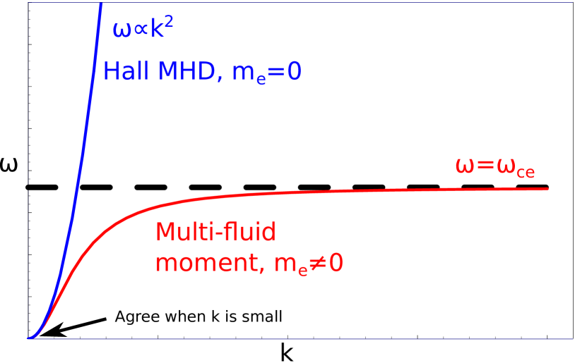
Figure 1: Dispersion curves for the whistler waves of the multi-fluid plasma model with finite electron mass (red curve), the Hall-MHD model with zero electron mass (blue curve). Finite electron inertia allows the whistler wave to have an asymptote at the electron cyclotron frequency (marked by the black horizontal dashed line) whereas ignoring electron inertia causes it to grow without bound as seen in the Hall-MHD model.

Sullivan et al.Sullivan, Bhattacharjee, and Huang (2009) performed a set of Hall MHD simulations with different $m_{e}$ to study the current sheet formation in a 2D coalescence problem, and found the scalings of the length and thickness of the electron current layer versus $m_{e}/m_{i}$. Here, we perform five-moment simulations of the same setup using different $m_{e}/m_{i}$ as well to find corresponding scalings in the five-moment model, and compare with their Hall MHD results.

The initial equilibrium is depicted in Fig.(1) of Ref. Sullivan, Bhattacharjee, and Huang, 2009, consisting of four flux tubes sustained by four out-of-plane current channels. A doubly periodic domain is employed, $-L/2<x,y<L/2$, where $L=12.8d_{i0}$, and $d_{i0}=c/\omega_{pi0}$ is the ion inertia length based on a characteristic density $n_{0}$. For convenience, the equilibrium setup is summarized below:

$$B_{x} = \left(2\pi/12.8\right)B_{x0}\sin\left(2\pi x/L\right)\cos\left(2\pi y/L\right),$$ (29)

$$B_{y} = \left(2\pi/12.8\right)B_{x0}\cos\left(2\pi x/L\right)\sin\left(2\pi y/L\right),$$ (30)

$$n = n_{0}\left[1+\frac{B_{x0}^{2}-B^{2}}{2\mu_{0}n_{0}k_{B}\left(T_{i}+T_{e}\right)}\right].$$ (31)

Here, $T_{e}=T_{i}=B_{x0}^{2}/2\mu_{0}n_{0}k_{B}$, and $B_{x0}$ is chosen such that $v_{Ax0}\equiv\sqrt{B_{x0}^{2}/\mu_{0}n_{0}m_{i}}=0.1c$. Ions are then perturbed to stream into the X-point along the anti-diagonal direction at the following velocity:

$$\delta\mathbf{u}_{i} = u_{0}\left[\sin\left(2\pi y/L\right)\hat{\mathbf{x}}+\sin\left(2\pi x/L\right)\hat{\mathbf{y}}\right],$$ (32)

where $u_{0}=0.1v_{Ax0}$. These ion flows bring the two anti-diagonal flux tubes towards each other, and form a current sheet at the X-point along diagonal direction. We will test four different electron mass ratios, $m_{e}/m_{i}=1/25$, $1/100$, $1/256$, and $1/400$.

The typical evolution of this system is that the current layer shrinks in both length and thickness before forming a stable structure around $t=10\Omega_{ci}^{-1}$. The time dependences of lengths and thickneses of the electron current layers in the Hall MHD simulations can be found in the top panels of Fig.(11) and (13) of Ref. Sullivan, Bhattacharjee, and Huang, 2009. Our five-moment simulations turn out produce qualitatively very similar time dependences. In the following study, we will focus on the later quasi-steady stages of different five-moment runs, when lengths and thicknesses of the electron current layers remain stable.

Fig. 2 shows the color contours of out-of-plane electron current density, $J_{z,e}$, in the quasi-steady states from different runs. There is a clear transition from the thick, diffusive, and relatively more elongated current layer for the case of $m_{e}/m_{i}=1/25$ (top-left), to the short, X-like structure for the case of $m_{e}/m_{i}=1/400$ (bottom right), bridged by the intermediate pictures of $m_{e}/m_{i}=1/100$ (top right) and $1/256$ (bottom left). This transition qualitatively agrees with the Hall MHD simulations, shown in Fig.(2 and 3) of Ref. Sullivan, Bhattacharjee, and Huang, 2009. The recovery of the X-like structure in the five-moment run with $m_{e}/m_{i}=1/400$ confirms that this run is approaching the limit of Hall MHD with $m_{e}=0$, since such structure is typically seen in Hall MHD simulations with $m_{e}=0$.

Fig. 3 shows the scalings of median stable plateau values of $L_{e}$ vs $m_{e}/m_{i}$ (left panel), and median stable plateau values of $\delta_{e}$ vs $m_{e}/m_{i}$ (right panel). Here, the length of the current layer, $L_{e}$, is defined by the distance between the peaks of electron outflow velocities, $u_{x,e}$, and the thickness, $\delta_{e}$, is the full width at half maximums of $J_{z,e}$. In both panels of Fig. 3, the solid squares, diamonds, triangle, and circles denote data from runs with $m_{e}/m_{i}=1/25$, $1/100$, $1/256$, and $1/400$, respectively. The dashed line in the left panel represents an estimated scaling $L_{e}\propto\left(m_{e}/m_{i}\right)^{3/8}$. The cross on the lower left end denotes an extrapolated value of $L_{e}\sim 12\text{ to }17d_{e0}$, or $0.28\text{ to }0.4d_{i0}$, for a physical mass ratio, $m_{e}/m_{i}=1/1836$. In the right panel, the dashed line represents an estimated scaling $\delta_{e}\propto\left(m_{e}/m_{i}\right)^{1/3}$, where the cross denotes an extrapolated value of $\delta_{e}\sim 0.4\text{ to }0.6d_{e0}$ for the physical mass ratio. Equivalent scalings from Hall MHD simulations are shown in the bottom panels of Fig(11) and (13) of Ref. Sullivan, Bhattacharjee, and Huang, 2009. The extrapolated values of $L_{e}$ are in good agreement, but the Hall MHD simulations predicted a significantly larger $\delta_{e}\sim 1d_{e0}$.

It should be clarified that, Sullivan et al. used a hyperresistivity in their Hall MHD simulations to break the frozen-flux constraint (necessary when $m_{e}=0$) and to maintain numerical stability, while our five-moment code does not include such a term. The hyperresistivity can control the length of the current sheetChacón, Simakov, and Zocco (2007); Sullivan, Bhattacharjee, and Huang (2009). However, when Sullivan et al. studied the effects of electron inertia, a tiny, fixed hyperresistivity was used in different runs, thus the influences on different runs due to this term should be similar and relatively small. Meanwhile, isothermal EoS were employed in their Hall MHD simulations, while the energy equations evolved in our five-moment simulation essentially indicate adiabatic EoS. Taking into account such inconsistencies between the numerical codes, and also the possible measurement errors due to the limited number of data points and the vast range of $m_{e}/m_{i}$ to be fitted, the overall agreements between the five-moment and the Hall MHD simulations are remarkably good.

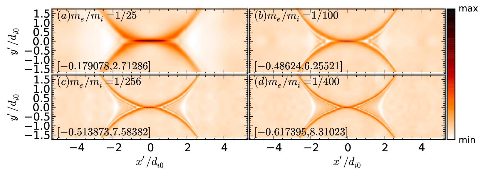
Figure 2: Out-of-plane electron current, $J_{z,e}$, in the unit of $n_{0}\left|e\right|v_{Ax0}$ from the five-moment simulations motivated by Sullivan et al.Sullivan, Bhattacharjee, and Huang (2009). Different panels correspond to different mass ratios, $m_{e}/m_{i}$, as marked at upper left of each panel. The values in lower right square brackets indicate the range of $J_{z,e}$ values within the region shown.

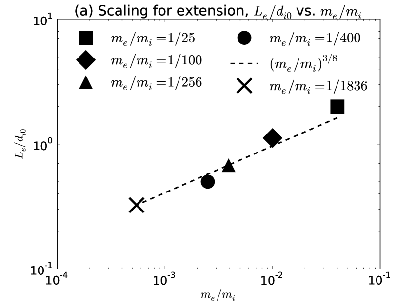
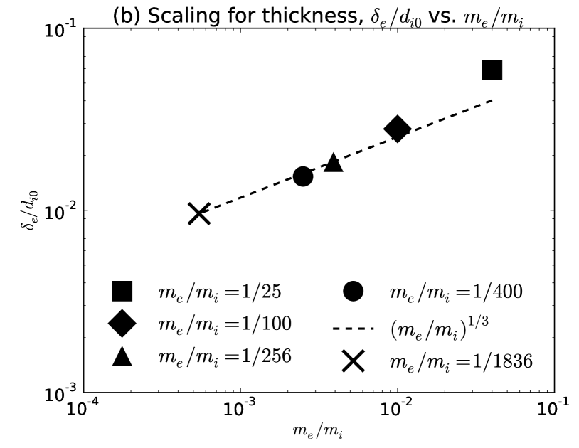
Figure 3: Left: $L_{e}/d_{i0}$ vs. $m_{e}/m_{i}$. The solid squares, diamonds, triangles, and circles represent five-moment simulations with $m_{e}/m_{i}=1/25$, $1/100$, $1/256$, and $1/400$, respectively. The dashed line indicates an estimated scaling $\sim(m_{e}/m_{i})^{3/8}$, with the black cross on the lower left end marking an extrapolated value of $L_{e}/d_{i0}$, for $m_{e}/m_{i}=1/1836$. Right: $\delta_{e}/d_{i0}$ vs. $m_{e}/m_{i}$. The dashed line indicates an estimated scaling of $(m_{e}/m_{i})^{1/3}$, with the black cross marking an extrapolated value of $\delta_{e}//d_{i0}$ for $m_{e}/m_{i}=1/1836$.

VI 2D Anti-Parallel Reconnection In A Harris Sheet

In this section, we investigate the ten-moment limit of the multi-fluid moment model, particularly its capability of evolving full electron pressure tensor, $\mathbf{P}_{e}$. To this end, ten-moment simulations are performed of 2D anti-parallel reconnection in a Harris sheet. We examine the roles of $\mathbf{P}_{e}$, in controlling the structures of electron current layer, and in supporting the reconnection electric field near the X-point. For comparison, PIC and five-moment simulations are performed with the same setup. The PIC simulation is fully kinetic, while the five-moment simulation permits scalar pressures only. The transition from five-moment to ten-moment and then to PIC thus forms a complete set of comparison. The PIC simulation are performed using the numerical code PSCGermaschewski et al. (sics).

Two ten-moment simulations are performed, with $k_{e0}=k_{i0}=1/10^{-4}d_{e0}$ and $1/d_{e0}$, respectively, where $d_{e0}$ is the electron inertia length due to an asymptotic number density $n_{0}$. $k_{e0}$ and $k_{i0}$ are the constant wave-numbers defining electron and ion heat-flux approximations in the form of Eq. (24). The $k_{e0}=k_{i0}=1/10^{-4}d_{e0}$ run approximates the limit of $k_{e0},k_{i0}\to\infty$, approaching the five-moment model. The $k_{e0}=k_{i0}=1/d_{e0}$ run, instead, aims at approaching the PIC run. $k_{e0}$ and $k_{i0}$ are chosen so as to approximately capture the characteristic length scale near the X-point, since previous studies of similar problems indicated that the electron current layer tends to thin down to a thickness comparable to $d_{e0}$. Our primary task is then to find the similarities and differences between this particular ten-moment run and the PIC run. For convenience, we call this run the targeted run in the rest of this study.

VI.1 Numerical setup

We employ a 2D simulation domain that is periodic in $x$ ($-L_{x}/2<x<L_{x}/2$) and is bounded by conducting walls in $y$ at $y=\pm L_{y}/2$. Here $L_{x}=100d_{i0}$, $L_{y}=50d_{i0}$, where $d_{i0}=\sqrt{m_{i}/\mu_{0}n_{0}\left|e\right|^{2}}$ is the ion inertia length due to $n_{0}$. The initial equilibrium is a single Harris sheet where magnetic field and number densities are specified by

$$\mathbf{B}_{0}=B_{0}\tanh\left(y/\lambda_{B}\right)\hat{\mathbf{x}},$$ (33)

and

$$n_{e}=n_{i}=n_{0}\text{sech}^{2}\left(y/\lambda_{B}\right)+n_{b},$$ (34)

respectively. The total current, $\mathbf{J}_{0}=\nabla\times\mathbf{B}_{0}/\mu_{0}$, is decomposed according to $J_{ze0}/J_{zi0}=T_{i0}/T_{e0}$, where the initial temperatures $T_{e0}$ and $T_{i0}$ are constant. A sinusoid perturbation is then applied on the magnetic field according to $\delta\mathbf{B}=\hat{\mathbf{z}}\times\nabla\psi$, where

$$\psi=\delta\psi\cos\left(2\pi x/L_{x}\right)\cos\left(\pi y/L_{y}\right).$$ (35)

The characterizing parameters follow Daughton, Scudder, and Karimabadi (2006), and are listed in Table 1 for convenience. Length, time, speed, and magnetic field strength are normalized over $d_{i0}$, $\Omega_{ci0}^{-1}$, and $v_{A0}$, respectively, where $B_{0}$ defines the ion cyclotron frequency $\Omega_{ci0}=eB_{0}/m_{i}$ and Alfvén speed $v_{A0}=B_{0}/\sqrt{\mu_{0}n_{0}m_{i}}$. The resolutions for five- and ten-moment runs are $4095\times 2047$, about $8$ cells per $d_{e0}$. The PIC run employs a $5760\times 2880$ grid ($12$ cells per $d_{e0}$) populated by about $2.7\times 10^{9}$ particles from each species, and resolves Debye length.

Reconnection in the setup described above has been extensively studied using various numerical models and with different parameterset al. (2001); Daughton, Scudder, and Karimabadi (2006); Schmitz and Grauer (2006); Hesse and Winske (1993); Kuznetsova, Hesse, and Winske (2001); Yin et al. (2001). Particularly, as mentioned in Sec.I, Hesse et al.Hesse and Winske (1993, 1994); Kuznetsova, Hesse, and Winske (2001) and Yin et al.Yin et al. (2001, 2002); Yin and Winske (2003) studied similar systems using modified hybrid and Hall MHD codes that evolve full $\mathbf{P}_{e}$ with help of a relaxation term. Our study differs from theirs in the following important aspects. First, as discussed in Sec.I and Sec.III, the underlying physical justification of their relaxation term is fundamentally different from ours. Second, their studies were limited to smaller system sizes. Another interesting study was the Vlasov simulation by Schmitz and GrauerSchmitz and Grauer (2006), in which the Vlasov equations are directly evolved, retaining full kinetic effects. Though their study also used small domain sizes ($25.6d_{i0}\times 12.8d_{i0}$), it agrees well in certain details with our larger targeted and PIC runs (particularly the latter), as we will show.

Parameter	$L_{x}/d_{i0}$	$L_{y}/d_{i0}$	$m_{i}/m_{e}$	$v_{A0}/c$	$2\mu_{0}n_{0}k_{B}\left(T_{i0}+T_{e0}\right)/B_{0}^{2}$	$n_{b}/n_{0}$	$T_{i0}/T_{e0}$	$\lambda_{B}/d_{i0}$	$\delta\psi/B_{0}d_{i0}$
Value	$100$	$50$	$25$	$1/15$	$1$	$0.3$	$5$	$0.913$	$0.1$

Table 1: Summary of parameters for simulations of the Harris sheet reconnection problem.

VI.2 Reconnected flux

The reconnected fluxes, $\Delta\psi$, are presented in Figure (4). Here, $\Delta\psi$ is calculated by integrating $d\psi=-\left|B_{y}\right|dx/2$ from the left boundary center to the right boundary center, and is normalized over $B_{0}d_{i0}$. The slope of a $\Delta\psi-t$ curve, $\partial\Delta\psi/\partial t$, is called the reconnection rate.

In Fig. 4, the different curves do not agree well with one another when $\Delta\psi$ rises significantly (indicating onset of reconnection) and and overall slope (indicating the average reconnection rate). These discrepancies could be caused by the different natures of PIC and multi-fluid moment models (in terms of certain microinstabilities, for example), and also by the presence of plasmoids. As will be visualized in Sec.VI.3, plasmoids are readily generated in the five-moment run (dashed curve) and the ten-moment runs with $k_{e0}=k_{i0}=1/10^{-4}d_{e0}$ (dashed-dotted curve). Plasmoids accelerate reconnection and lead to early rise of $\Delta\psi$. In comparison, the targeted run (fine dotted curve) appears to be marginally stable to plasmoids, where tiny plasmoids appear only very transiently around $t=150\Omega_{ci0}^{-1}$ and are immediately merged, corresponding to a much more gentle slope with a tiny “bump” around $t=150\Omega_{ci0}^{-1}$. Finally, the PIC run (solid curve) shows no plasmoid at all and has the most gentle slope.

Though the physics of plasmoids is not the primary concern in this study, it modifies time dependences of reconnected fluxes significantly. Thus, when comparing different runs, we should select frames when the same amount of fluxes are newly reconnected, i.e., when $\Delta\psi-\Delta\psi\left(t=0\right)$ are the same. In such time frames, different runs might be considered in a similar stage of the evolution. We will follow this criterion to select comparable frames in the rest of this study.

Figure 4: Reconnected flux $\Delta\psi$ vs. time from simulations of the Harris sheet reconnection problem using different models.

VI.3 Structures of electron current layer

Fig. 5 shows snapshots of electron out-of-plane velocities, $u_{z,e}$, near the domain centers. These snapshots are taken at times when $\Delta\psi-\Delta\psi\left(t=0\right)\approx 2.5B_{0}d_{i0}$. It is readily seen that the five-moment run (Panel (b)) and ten-moment run with $k_{e0}=k_{i0}=1/10^{-4}d_{e0}$ (Panel (c)) generate a chain of plasmoids, and are remarkably similar to each other. Such similarity is not surprising, since the ten-moment run with $k_{e0}=k_{i0}=1/10^{-4}d_{e0}$ approaches the five-moment limit. The immediate generation of plasmoid chains also indicates that, in these two simulations, electron inertia alone is not sufficient to prevent the electron current layer from rapidly thinning down to the $d_{e0}$ scale.

The targeted run (Panel (d)), in comparison, contains no plasmoid at this time, and is rather similar to the PIC result (Panel (a)) in terms of lengths and thicknesses of the current layers, magnitudes of the maximum $u_{z,e}$, and opening angles of the separatrices. It should be pointed out that the frames shown here might not be precisely timed when $\Delta\psi-\Delta\psi\left(t=0\right)=2.5$ due to limited frames of data points. Taking into account such possible offsets in timing, the agreement between the targeted run and the PIC run appears to be reasonably good.

The agreement between the PIC run and the targeted run can be further confirmed by Fig. 6 that shows cuts of electron flows velocities along inflow and outflow lines from the targeted run (dashed curves) and the PIC run (solid curves) earlier when $\Delta\psi-\Delta\psi\left(t=0\right)=2$. Top and middle panels show outflow electron velocities, $u_{x,e}$, and out-of-plane electron velocities, $u_{z,e}$, along outflow direction. The two runs agree very well near the central X-point, but the magnitudes in the PIC run fall faster in the further downstream “lobe” regions. Bottom panel shows $u_{z,e}$ along inflow lines, where the two runs are remarkably similar. This set of comparisons is repeated in later time frames when $\Delta\psi-\Delta\psi\left(t=0\right)=3.75$, shown in Fig. 7. Similar agreement is observed again in Fig. 7.

The excellent agreement between the targeted and PIC runs near the X-point indicates that the choice of $k_{e0}=k_{i0}=1/d_{e0}$ indeed correctly handles the dominating physical length scales near the X-point. The discrepancies in the further downstream lobe regions imply that $k_{e0}=k_{i0}=1/d_{e0}$ is less appropriate in these regions, since the characteristic length scales grow larger, as indicated by the opening of separatrices. Consequently, $k_{e0}$ and $k_{i0}$ should be reduced accordingly in those regions.

Figure 5: Color contours of out-of-plane electron velocity, $u_{z,e}$, in simulations of the Harris sheet reconnection problem using different models. The frames are selected when $\Delta\psi-\Delta\psi\left(t=0\right)\approx 2.5$.

Figure 6: Cuts of electron velocities in the PIC run and ten-moment run with $k_{e0}=k_{i0}=1/d_{e0}$ of the Harris sheet reconnection problem. Top panel is the outflow electron velocities, $u_{x,e}$, along outflow lines. Middle panel is the out-of-plane electron velocities, $u_{z,e}$, along outflow lines. Bottom panel is $u_{z,e}$ along inflow lines. Data are at sampled time when $\Delta\psi-\Delta\psi\left(t=0\right)\approx 2$. Note that the PIC data are slightly shifted along the outflow line to place the stagnation point right at the domain center.

Figure 7: Repeatition of Fig. 6 when $\Delta\psi-\Delta\psi\left(t=0\right)\approx 3.75$.

VI.4 Relaxation of pressure tensor in the ten-moment model

Next, we compare the full pressure tensors from PIC and ten-moment simulations. This side-by-side comparison directly evaluates the capability of the ten-moment model to organize the non-gyrotropic, anisotropic pressure tensors. We should also keep in mind that calculating higher order moments like the pressure tensor in a PIC simulation is not trivial, since the data are noisy in nature due to fluctuations of discrete computational particles.

Fig. 8 shows diagonal elements of $\mathbf{P}_{e}$ from the PIC run (first row), the targeted run (second row), and the ten-moment run with $k_{e0}=k_{i0}=1/10^{-4}d_{e0}$ (bottom row). The data are sampled early in the quasi-steady states when $\Delta\psi-\Delta\psi\left(t=0\right)=1$. The global structures of different terms are in agreement between the PIC and targeted run. The maximum value of $P_{xx,e}$, $P_{yy,e}$, and $P_{zz,e}$ in the PIC run are $0.224$, $0.167$, and $0.186$ in units of $B_{0}^{2}/\mu_{0}$, obeying the relation $P_{xx,e,max}>P_{zz,e,max}\gtrsim P_{yy,e,max}$. This relation was also found by previous Vlasov simulation (Fig.(5) of Ref. Schmitz and Grauer, 2006) on a smaller domain. The corresponding maximums are $0.25$, $0.239$, and $0.232$ in the targeted run, obeying a slightly different relation $P_{xx,e,max}\gtrsim P_{zz,e,max}\approx P_{yy,e,max}$. In other word, the targeted run generates slightly more isotropy than fully kinetic simulations, which might be improved by a better collisionless closure in the full 3D regime. In comparison, the three diagonal elements are almost identical in the ten-moment run with $k_{e0}=k_{i0}=1/10^{-4}d_{e0}$, since it approaches the isotropic five-moment limit.

Fig. 9 shows off-diagonal elements of $\mathbf{P}_{e}$ from the PIC run (top row) and targeted run (bottom row). The results from the ten-moment run with $k_{e0}=k_{i0}=1/10^{-4}d_{e0}$ are not shown here because the off-diagonal elements vanish (almost to level of machine error) as a result of strong gyrotropization. As shown in Fig. 9, the overall structures, particularly the polarities of these off-diagonal elements in the PIC run are very well recovered in the targeted run. However, the relations between magnitudes of terms in different locations do not agree well. For the quadrupole-shaped $P_{xy,e}$ (first column), the maximum magnitude in the PIC run ($\sim 0.024$) is four times that in the targeted run ($\sim 0.006$). For $P_{xz,e}$ (second column), the magnitudes near the X-point are close ($\sim 0.014$); but in the further downstream lobe regions, the magnitudes grow to $\sim 0.03$ in the PIC run, but decay to much smaller values in the targeted run run in the same regions. For $P_{yz,e}$ (third column), the magnitudes near the X-point are $\sim 0.005$ in PIC run, smaller than that in targeted run ($\sim 0.01$); the magnitudes grow in the lobe regions in PIC run to $\sim 0.016$, but decay to very small values in Targed. On the other hand, the small domain Vlasov simulation (Fig.(6) of Ref. Schmitz and Grauer, 2006), again, showed structures and magnitude relations of these off-diagonal elements very similar to our PIC run.

From the above comparisons, it is clear that the ten-moment run with $k_{e0}=k_{i0}=1/10^{-4}d_{e0}$ indeed relaxes the full $\mathbf{P}_{e}$ to a scalar, which is essentially the five-moment limit. It is also clear that the targeted ten-moment run with $k_{e0}=k_{i0}=1/d_{e0}$ recovers well the full tensor $\mathbf{P}_{e}$ around the X-point. It does less well in the further downstream lobe regions, though. On the other hand, though limited by small domain size, previous fully kinetic Vlasov simulation agrees with the PIC run and the targeted run in overal structures of various terms, and also demonstrates certain quantitative relations that are close to our PIC run.

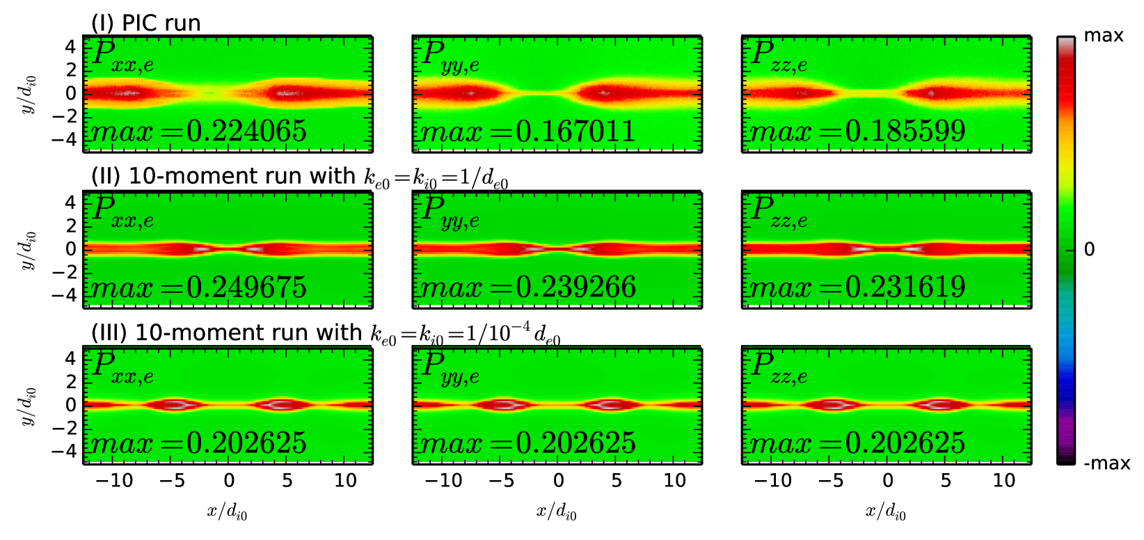
Figure 8: Color contours of diagonal elements of $\mathbf{P}_{e}$ sampled when $\Delta\psi-\Delta\psi\left(t=0\right)=1$. The three rows (top to bottom) are from the PIC run, the targeted run, and the ten-moment run with $k_{e0}=k_{i0}=1/10^{-4}d_{e0}$, respectively. The three columns (left to right) correspond to $P_{xx,e}$, $P_{yy,e}$, and $P_{zz,e}$, respectively.

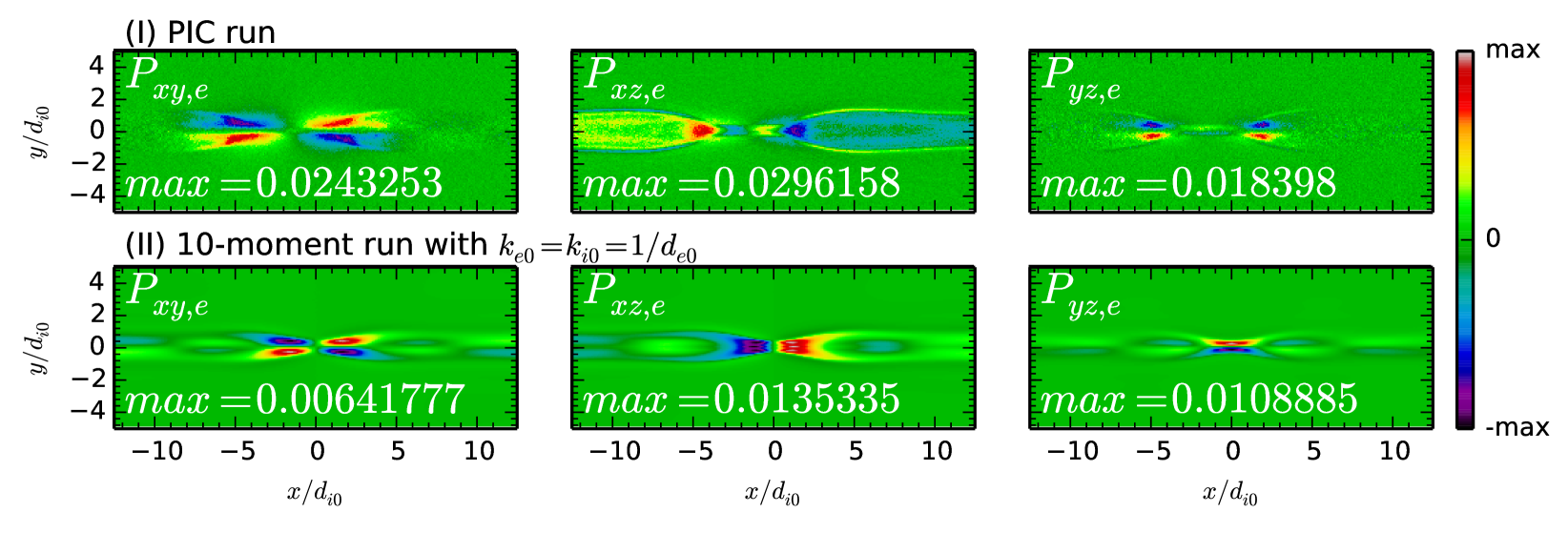
Figure 9: Color contours of diagonal elements of $\mathbf{P}_{e}$ sampled when $\Delta\psi-\Delta\psi\left(t=0\right)=1$. The top row is from the PIC run, and the bottom row is from the targeted run. The three columns (left to right) correspond to $P_{xy,e}$, $P_{yz,e}$, and $P_{xz,e}$, respectively.

VI.5 Decomposition of the Ohm’s law

The capability of the ten-moment model to evolve full $\mathbf{P}_{e}$ can also be investigated by decomposing the following form of generalized Ohm’s law (essentially the electron momentum equation) around the reconnection site:

$$E_{z} = -u_{x,e}B_{y}+u_{y,e}B_{x}-\frac{1}{n_{e}\left|e\right|}\left(\frac{\partial P_{xz,e}}{\partial x}+\frac{\partial P_{yz,e}}{\partial y}\right)$$ (36)

$$-\frac{1}{n_{e}\left|e\right|}\left[\frac{\partial}{\partial t}\left(m_{e}n_{e}u_{z,e}\right)+\frac{\partial}{\partial x}\left(m_{e}n_{e}u_{x,e}u_{z,e}\right)\right.$$

$$\left.+\frac{\partial}{\partial y}\left(m_{e}n_{e}u_{y,e}u_{z,e}\right)\right].$$

In a 2D setup, the reconnection rate can be measured by $\left|E_{z}\right|\approx\partial\psi/\partial t$ at the reconnection site, which is an important diagnosticVasyliunas (1975). Historically, PIC and traditional fluid simulations of 2D anti-parallel reconnection showed vast differences in the sources of $E_{z}$ at the X-point. PIC simulations showed that $E_{z}$ is largely supported by the divergence of the off-diagonal elements of $\mathbf{P}_{e}$, i.e., $E_{z}^{\text{ng}}\equiv-\left(\partial_{x}P_{xze}+\partial_{y}P_{yze}\right)/n_{e}\left|e\right|$, while traditional fluid models only permit a scalar pressure, $p_{e}$, which does not contribute to $E_{z}^{\text{ng}}$. It is thus interesting to find the contribution of $E_{z}^{ng}$ to $E_{z}$ in ten-moment simulations to see if it is consistent with the PIC results.

Fig. 10 shows constituting terms of Eq.(36) along the outflow line in the PIC run (panel (a)) versus the targeted run (panel (b)). The sampling time is when $\Delta\psi-\Delta\psi\left(t=0\right)=2$. Red curves are $E_{z}$, and black dashed curves are sums of terms on the right-hand-side of equation (36), denoted by $E_{z,sum}$. In both runs, the magnitudes of $E_{z}$ are comparable, and are both dominated by $-\partial P_{yz,e}/\partial y$ (yellow-green curves) at the stagnation point where $E^{\text{convective}}\equiv-u_{x,e}B_{y}+u_{y,e}B_{x}=0$ (i.e., where green curves touch zero). This agreement cofirms that ten-moment run is evolving $\mathbf{P}_{e}$ qualitatively correctly. The structures of terms in Eq.(36) in the two runs are also similar. For example, in both runs, $E_{z}^{\text{ng}}$ overshoots in the further downstream regions with comparable magnitudes, while $-\partial P_{yz,e}/\partial y$ and $E^{\text{convective}}$ overshoot in opposite ways in the downstream regions.

A major difference is that, in the PIC run, the overshooting of $E_{z}^{\text{convective}}$ is largely cancelled by $-\partial P_{yz,e}/\partial y$, and the resulting $E_{z}$ is relatively flat, while in the targeted run, little cancellation was shown between the two terms because their peaks do not overlap. As a result, $E_{z}$ is dominated by $E_{z}^{\text{convective}}$ and in addition, shows overshoots in the downstream regions.

It should be emphasized that comparison of the various terms in the generalized Ohm’s law from different types of simulations is sensitive to the choice of when in time such comparisons are made. The inherent noises in the PIC simulation also make the measurement of various mean quantities subject to fluctuations. Considering these possible sources of errors, it is noteworthy that the generalized Ohm’s law in the ten-moment run can achieve rather good agreement with the PIC run, even with a simple closure (constant $k_{e0}=k_{i0}=1/d_{e0}$ in Eq. (24)).

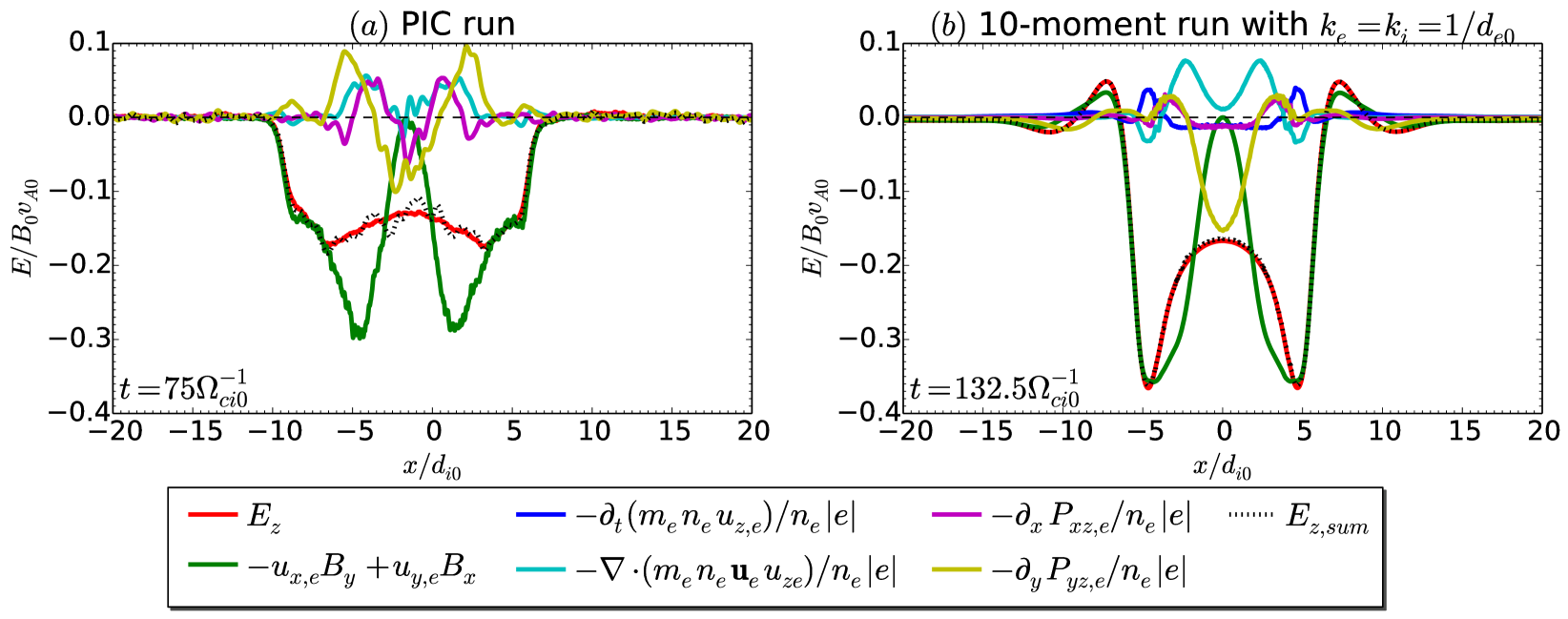
Figure 10: Terms consistituting the generalized Ohm’s law, Eq.(36), along the outflow line (i.e., $x$-axis) from the PIC (left panel) and the targeted run (right panel). The sampling time is when $\Delta\psi-\Delta\psi\left(t=0\right)=2$.

VII Conclusions and Future Work

We have investigated the multi-fluid moment model in the context of collisionless magnetic reconnection. Two limits of this model were discussed: the five-moment limit that evolves scalar pressures, and the ten-moment limit that evolves full pressure tensors. First, through the example of the five-moment model, we demonstrated how effects critical in collisionless reconnection are self-consistently embedded, and how the resulting five-moment equations formally approach the more widely used Hall MHD equations under the limits of vanishing electron inertia, infinite speed of light, and quasi-neutrality. Then, we investigate the capability of the ten-moment model to evolve full pressure tensors. In order to approach fully kinetic models, we implemented a local linear collisionless closure in the form of Eq. (24) to approximate (divergence of) the heat flux. This simple closure takes a characteristic wave-number, $k_{0}$, that is constant throughout the simulation domain to prescribe the scale at which collisionless Landau damping effectively occurs. When applied to Harris sheet reconnection, the ten-moment run using this crude closure and $k_{e}=k_{i}=1/d_{e0}$ (which we call the targeted run) yields elements of $\mathbf{P}_{e}$ that are consistent with the PIC results in the vicinity of the reconnection site, and reproduces electron flows that are remarkably similar to the PIC ones. In the further downstream lobe regions, however, the agreement is less satisfactory. In addition, near the X-point, subtle, but noticeable differences in magnitude relations between different elements of $\mathbf{P}_{e}$ are also observed.

The discrepancies between the targeted ten-moment run and the PIC run indicate the need to determine closure parameters, $k_{e0}$ and $k_{i0}$, from local properties (e.g., scales of local gradients), and the need for a better closure in the full 3D regime (instead of using the same $k_{e0}$ and $k_{i0}$ for every direction). As a step to improve the closure to suit such needs, analytic generalization of Eq. (24) is necessary, which will require non-trivial mathematical manipulations. Methods mentioned in Sec.III to perform non-local integration through Hilbert transform of the temperature may also be benchmarked. On the other hand, in order to better understand properties of the heat flux, it is necessary to compare the approximated heat flux due to closures in ten-moment simulations with the real heat flux from fully kinetic simulations, and possibly with heat flux calculated in a twenty-moment model (not implemented yet) which evolves full (fourth-order) heat flux tensor. The different ways summarized above to improve the collisionless closure are left to future work.

The ten-moment model is very attractive for global modeling of large scale collisionless systems like the Earth’s and other planetary magnetospheres. First, the ten-moment model avoids two well-known deficiencies of popular MHD-based magnetospheric codes, namely, the lack of full electron pressure tensor, and the difficulty in effeciently incorporating the Hall term. In the ten-moment model, both terms (together with other terms like electron inertia) are self-consistently embedded, and can be easily implemented using a locally implicit algorithm that eliminates time step restriction due to quadratic dispersive modes. On the other hand, the multi-fluid moment model can easily handle multiple species, which facilitates modeling of situations where multi-ion-species plays a significant role. In future work, the ten-moment moment model can be either directly implemented as a base model for global simulations, or be integrated in an existing global code to capture necessary physics in localized regions.

To conclude, the multi-fluid moment model provides an alternative approach to include non-ideal, but collisionless effects in a continuum code. With a seemingly crude, but physically fundamental closure in the form of Eq. (24), the ten-moment model can evolve $\mathbf{P}_{e}$ largely correct when appropriate closure parameters are chosen. In future work, different approaches to improve the collisionless closure should be explored, towards a fully 3D, non-local closure. Direct application of the ten-moment model to magnetosphere should also be sought, and could be a crucial step towards integration of kinetic effects in global magnetospheric models.

References

- Yamada, Kulsrud, and Ji (2010) M. Yamada, R. Kulsrud, and H. Ji, Reviews of Modern Physics 82, 603 (2010).
- Zweibel and Yamada (2009) E. G. Zweibel and M. Yamada, Annual Review of Astronomy & Astrophysics 47, 291 (2009).
- Sweet (1958) P. A. Sweet, in Electromagnetic Phenomena in Cosmical Physics, IAU Symposium, Vol. 6, edited by B. Lehnert (1958) p. 123.
- Parker (1957) E. N. Parker, Journal of Geophysical Research 62, 509 (1957).
- Ji et al. (1999) H. Ji, M. Yamada, S. Hsu, R. Kulsrud, T. Carter, and S. Zaharia, Physics of Plasmas 6, 1743 (1999).
- Trintchouk et al. (2003) F. Trintchouk, M. Yamada, H. Ji, R. M. Kulsrud, and T. A. Carter, Physics of Plasmas 10, 319 (2003).
- Øieroset et al. (2001) M. Øieroset, T. D. Phan, M. Fujimoto, R. P. Lin, and R. P. Lepping, Nature 412, 414 (2001).
- Egedal et al. (2000) J. Egedal, A. Fasoli, M. Porkolab, and D. Tarkowski, Review of Scientific Instruments 71, 3351 (2000).
- Vasyliunas (1975) V. M. Vasyliunas, Reviews of Geophysics and Space Physics 13, 303 (1975).
- et al. (2001) J. B. et al., Journal of Geophysical Research 106, 3715 (2001).
- Ma and Bhattacharjee (1998) Z. W. Ma and A. Bhattacharjee, Geophysical Research Letters 25, 3277 (1998).
- Wang, Bhattacharjee, and Ma (2000) X. Wang, A. Bhattacharjee, and Z. W. Ma, Journal of Geophysical Research 105, 27633 (2000).
- Cai and Lee (1997) H. J. Cai and L. C. Lee, Physics of Plasmas 4, 509 (1997).
- Kuznetsova, Hesse, and Winske (2001) M. M. Kuznetsova, M. Hesse, and D. Winske, Journal of Geophysical Research 106, 3799 (2001).
- Kuznetsova, Hesse, and Winske (1998) M. M. Kuznetsova, M. Hesse, and D. Winske, Journal of Geophysical Research 103, 199 (1998).
- Bowers et al. (2008) K. J. Bowers, B. J. Albright, L. Yin, B. Bergen, and T. J. T. Kwan, Physics of Plasmas 15, 055703 (2008).
- Germaschewski et al. (sics) K. Germaschewski, W. Fox, N. Ahmadi, L. Wang, S. Abbott, H. Ruhl, and A. Bhattacharjee, ArXiv e-prints (To be submitted to Journal of Computational Physics), arXiv:1310.7866 [physics.plasm-ph] .
- Lapenta (2012) G. Lapenta, Journal of Computational Physics 231, 795 (2012).
- Raeder, Berchem, and Ashour-Abdalla (1998) J. Raeder, J. Berchem, and M. Ashour-Abdalla, Journal of Geophysical Research 103, 14787 (1998).
- Tóth et al. (2005) G. Tóth, I. V. Sokolov, T. I. Gombosi, D. R. Chesney, C. R. Clauer, D. L. de Zeeuw, K. C. Hansen, K. J. Kane, W. B. Manchester, R. C. Oehmke, K. G. Powell, A. J. Ridley, I. I. Roussev, Q. F. Stout, O. Volberg, R. A. Wolf, S. Sazykin, A. Chan, B. Yu, and J. Kóta, Journal of Geophysical Research (Space Physics) 110, A12226 (2005).
- Lipatov (2002) A. S. Lipatov, The Hybrid Multiscale Simulation Technology, Scientific Computation (Springer Berlin Heidelberg, Berlin, Heidelberg, 2002).
- Hesse and Winske (1993) M. Hesse and D. Winske, Geophysical Research Letters 20, 1207 (1993).
- Hesse and Winske (1994) M. Hesse and D. Winske, Journal of Geophysical Research 99, 11177 (1994).
- Hesse, Winske, and Kuznetsova (1995) M. Hesse, D. Winske, and M. M. Kuznetsova, Journal of Geophysical Research 100, 21815 (1995).
- Gary, Winske, and Hesse (2000) S. P. Gary, D. Winske, and M. Hesse, Journal of Geophysical Research 105, 10751 (2000).
- Kuznetsova, Hesse, and Winske (2000) M. M. Kuznetsova, M. Hesse, and D. Winske, Journal of Geophysical Research 105, 7601 (2000).
- Yin et al. (2001) L. Yin, D. Winske, S. P. Gary, and J. Birn, Journal of Geophysical Research 106, 10761 (2001).
- Yin et al. (2002) L. Yin, D. Winske, S. P. Gary, and J. Birn, Physics of Plasmas 9, 2575 (2002).
- Yin and Winske (2003) L. Yin and D. Winske, Physics of Plasmas 10, 1595 (2003).
- Sugiyama and Kusano (2007) T. Sugiyama and K. Kusano, Journal of Computational Physics 227, 1340 (2007).
- Daldorff et al. (2014) L. K. S. Daldorff, G. Tóth, T. I. Gombosi, G. Lapenta, J. Amaya, S. Markidis, and J. U. Brackbill, Journal of Computational Physics 268, 236 (2014).
- Le et al. (2009) A. Le, J. Egedal, W. Daughton, W. Fox, and N. Katz, Physical Review Letters 102, 085001 (2009).
- Le et al. (2010) A. Le, J. Egedal, W. Fox, N. Katz, A. Vrublevskis, W. Daughton, and J. F. Drake, Physics of Plasmas 17, 055703 (2010).
- Ohia et al. (2012) O. Ohia, J. Egedal, V. S. Lukin, W. Daughton, and A. Le, Physical Review Letters 109, 115004 (2012).
- Egedal, Le, and Daughton (2013) J. Egedal, A. Le, and W. Daughton, Physics of Plasmas 20, 061201 (2013).
- Tóth, Ma, and Gombosi (2008) G. Tóth, Y. Ma, and T. I. Gombosi, Journal of Computational Physics 227, 6967 (2008).
- Chacón, Knoll, and Finn (2002) L. Chacón, D. A. Knoll, and J. M. Finn, Journal of Computational Physics 178, 15 (2002).
- (38) L. Chacon, “Efficient algorithms for fluid simulation of magnetized plasmas,” Workshop II: Computational Challenges in Magnetized Plasma, Institute for Pure and Applied Mathematics, UCLA, April 16-20, 2012.
- Jardin (2012) S. C. Jardin, Journal of Computational Physics 231, 822 (2012).
- Daglis et al. (1999) I. A. Daglis, R. M. Thorne, W. Baumjohann, and S. Orsini, Reviews of Geophysics 37, 407 (1999).
- Moore et al. (2001) T. E. Moore, M. O. Chandler, M.-C. Fok, B. L. Giles, D. C. Delcourt, J. L. Horwitz, and C. J. Pollock, Space Science Reviews 95, 555 (2001).
- Shumlak and Loverich (2003) U. Shumlak and J. Loverich, Journal of Computational Physics 187, 620 (2003).
- Loverich, Hakim, and Shumlak (2010) J. Loverich, A. Hakim, and U. Shumlak, Communications in Computational Physics (2010).
- Hakim, Loverich, and Shumlak (2006) A. Hakim, J. Loverich, and U. Shumlak, Journal of Computational Physics 219 (2006).
- Hakim (2008) A. H. Hakim, Journal of Fusion Energy 27, 36 (2008).
- Johnson (2013) E. A. Johnson, Gaussian-Moment Relaxation Closures for Verifiable Numerical Simulation of Fast Magnetic Reconnection in Plasma, Ph.D. thesis, University of Wisconsin, Madison (2013).
- Joh (2013) Two-fluid 20-moment simulation of fast magnetic reconnection (Society of Industrial and Applied Mathematics, Computational Science and Engineering Conference, Boston, MA, 2013).
- Hammett and Perkins (1990) G. W. Hammett and F. W. Perkins, Physical Review Letters 64, 3019 (1990).
- Buneman (1961) O. Buneman, The Physics of Fluids 4, 669 (1961).
- Chew, Low, and Goldberg (1956) G. Chew, F. Low, and M. Goldberg, Proc. Roy. Soc. (London) A236, 112 (1956).
- Srinivasan and Shumlak (2011) B. Srinivasan and U. Shumlak, Physics of Plasmas 18, 092113 (2011).
- Chang and Callen (1992) Z. Chang and J. D. Callen, Physics of Fluids B: Plasma Physics 4, 1167 (1992).
- Hammett, Dorland, and Perkins (1992) G. W. Hammett, W. Dorland, and F. W. Perkins, Physics of Fluids B 4, 2052 (1992).
- Snyder, Hammett, and Dorland (1997) P. B. Snyder, G. W. Hammett, and W. Dorland, Physics of Plasmas 4, 3974 (1997).
- Kinsey, Staebler, and Waltz (2008) J. E. Kinsey, G. M. Staebler, and R. E. Waltz, Physics of Plasmas 15, 055908 (2008).
- Goswami, Passot, and Sulem (2005) P. Goswami, T. Passot, and P. L. Sulem, Physics of Plasmas 12, 102109 (2005).
- Chust and Belmont (2006) T. Chust and G. Belmont, Physics of Plasmas 13, 012506 (2006).
- James (1997) J. W. James, Implementation and application of non-local parallel heat flow in magnetized plasmas, Ph.D. thesis, University of Utah (1997).
- dim (2012) Efficient non-fourier implementation of Landau-fluid operators in the BOUT++ Code (Americal Physical Society, Division of Plasma Physics, 2012).
- Greengard and Rokhlin (1987) L. Greengard and V. Rokhlin, Journal of Computational Physics 73, 325 (1987).
- Brackbill (2011) J. U. Brackbill, Physics of Plasmas 18, 032309 (2011).
- Hakim (2014) A. H. Hakim, Physics of Plasmas (2014), sumbitted for publication.
- Loverich et al. (2013) J. Loverich, S. C. D. Zhou, K. Beckwith, M. Kundrapu, M. Loh, S. Mahalingam, P. Stoltz, and A. Hakim, in 51st AIAA Aerospace Sciences Meeting including the New Horizons Forum and Aerospace Exposition (American Institute of Aeronautics and Astronautics, Reston, Virigina, 2013).
- Birdsall and Langdon (1990) C. Birdsall and A. B. Langdon, Plasma Physics Via Computer Simulation (Institute of Physics Publishing, 1990).
- LeVeque (2002) R. J. LeVeque, Finite Volume Methods For Hyperbolic Problems (Cambridge University Press, 2002).
- Roe (1981) P. Roe, Journal of Computational Physics 43, 357 (1981).
- Brown (1996) S. L. Brown, Ph.D Thesis, University of Michigan , 1 (1996).
- Bouchut (2004) F. Bouchut, Nonlinear stability of finite volume methods for hyperbolic conservation laws, and well-balanced schemes for sources, Frontiers in Mathematics (Birkh’́auser, 2004).
- Sullivan, Bhattacharjee, and Huang (2009) B. P. Sullivan, A. Bhattacharjee, and Y.-M. Huang, Physics of Plasmas 16, 102111 (2009), arXiv:0905.4765 [physics.plasm-ph] .
- Chacón, Simakov, and Zocco (2007) L. Chacón, A. Simakov, and A. Zocco, Physical Review Letters 99, 235001 (2007).
- Daughton, Scudder, and Karimabadi (2006) W. Daughton, J. Scudder, and H. Karimabadi, Physics of Plasmas 13, 072101 (2006).
- Schmitz and Grauer (2006) H. Schmitz and R. Grauer, Physics of Plasmas 13, 092309 (2006), physics/0608175 .